Bell measurement rules out supraquantum correlations

Abstract

The so called bipartite non-signaling boxes are systems whose statistics is constrained solely by the principle of no instantaneous signaling between distant locations. Such systems can exhibit much stronger correlations than those admitted by quantum mechanics. Inspired by quantum logic approach of Tylec and Kuś, J. Phys. A: Math. Theor. 48 (2015) 505303, we consider non-signaling boxes with three inputs per party, and extend the set of measurements with just a single global measurement - one that mimics quantum two-party Bell measurement. We then show that this seemingly mild extension completely rules out supraquantum correlations: the resulting system admits precisely quantum mechanical correlations of two qubits. We also consider non-maximally entangled measurements, obtaining interpolation between quantum and full no-signaling theory. Our study paves a way to a general programme of amending no-signaling theories with some measurements inherited from quantum mechanics, leading to various interpolations between non-signaling boxes and quantum mechanics.

I Introduction

The idea of non-signaling boxes introduced in PR has become very fruitful for several purposes. First, the non-signaling boxes have found an application to device-independent cryptography Barrett_crypto_Bell , basing solely on assumption of no instantaneous signaling and violation of Bell inequalities Bellreview . In particular, randomness amplification and expansion protocol have been proposed Pironio_rand_exp_Nature ; ColbeckRenner , whose verification does not require any knowledge on quantum mechanics, but can be done based solely on statistical behaviour of the devices. On the other hand, analysis of non-signaling boxes leads to a better understanding of capabilities and limitations of quantum theory itself: the set of quantum mechanical states forms a convex body situated between two polytopes: the classical polytope of Kolmogorovian probability distributions and the larger poytope of all non-signaling boxes. The concept of non-signaling boxes has lead to a vast field of so called General Probabilistic Theories (GPT) GPT1 ; GPT2 ; GPT3 .

Recently, the relations between GPT and quantum logic were analysed TylecKus . The authors use the framework of quantum logic to construct logic of propositions of two-party non-signaling boxes. They build the logic from propositions describing single party and prove that the logic indeed describe spatially separated subsystems.

So far within the subject of GPT, not much has been done regarding joint measurements on composite systems. Boxes with bipartite measurements were considered in hypersigVedral and were used to construct examples of theories violating ”no-hypersignaling principle” formulated therein. These measurements were based on extremal points of the no-signaling polytope. The resulting models either exhibit solely classical correlations (when measurements corresponding to all extremal points are added) or exhibit maximally non-local correlations - those violating Tsirelson bound Tsi . In this context, an important challenge is to build models that interpolate between the two extremes. For single system, an important example of such interpolation is family of polygonic models Massar-polygon some of them violating Holevo bound. A bipartite models based on polygonic local systems was also considered polygon-CHSH , some of them violating Tsirelson bound. Yet, the joint measurements possible for those systems have not been analyzed.

In this paper we want to to avoid the binary situation: classical or full nosingaling, hence we need more sophisticated measurements than ones used in hypersigVedral . To this end we take inspiration from the quantum logic approach to nosignaling boxes of Ref. TylecKus . We aim to analyse the effect of enriching the initial model - a standard no signaling-box, which admits just product measurements - with an entangled measurement inherited from quantum mechanics.

The basic global measurement in quantum mechanics one may think of is clearly the Bell measurement MBRevzen_Bell . Surprisingly, we obtain that adding just this single measurement severely constrains the set of possible states. Namely, we show that the no-signaling box with Bell measurement exhibits no supraquantum correlations. It actually reproduces exactly all quantum correlations. We do it by showing that existence of Bell measurement, combined with natural assumption, that product of local states is a legitimate joint state, imposes that local states form a ball, i.e. it is the same as the set of states of qubit. Then we use the result of LQandNS where it is shown, that bipartite systems which are locally quantum, and are no-signaling, admit only quantum correlations.

We also consider non-maximally entangled measurements, and obtain interpolation between local systems being balls (like in quantum mechanics) and cubes (i.e completely unrestricted local systems).

II Model

We consider system $\mathcal{S}_{AB}$ composed of two elementary subsystems $\mathcal{S}_{A},\mathcal{S}_{B}$. State spaces of elementary systems $\mathcal{S}_{A}$ and $\mathcal{S}_{B}$ are identical.

The elementary system may be measured by means of one of three dichotomic measurements $X,Y,Z$. The measurements are not compatible, i.e. they cannot be measured together. In this sense they mimic Pauli measurements for quantum system. However at this step we do not put any constraints on the measurements outcomes probabilities beside standard positivity and normalisation constraints. In particular, there are no uncertainty constraints for elementary system.

The state of the elementary system $\mathcal{S}_{A}$ is described by probabilities of measurement outcomes: $p(a|x_{A})$, where $x_{A}\in\{X,Y,Z\}$ enumerates measurements and $a$ enumerates outcomes ”$+$”, ”$-$” (similarly for $\mathcal{S}_{B}$).

Now we move to composed system $\mathcal{S}_{AB}$. Consider first standard no-signaling bipartite boxes PR . These boxes are described by probabilities $p(ab|x_{A}x_{B})$ where $a\in\{+,-\}$ denote output of measurement $x_{A}\in\{X,Y,Z\}$ performed on subsystem $A$, analogically for $b$ and $x_{B}$. Probabilities $p(ab|x_{A}x_{B})$ fulfill non-signaling conditions, i.e. probability of outcomes of measurement performed on subsystem $A$ do not depend on the measurement performed on the subsystem $B$ (analogically for $B$ and $A$). The condition is expressed by equation:

$$\sum_{b}p(a,b|x_{A},x_{B})=\sum_{b}p(a,b|x_{A},x_{B}^{\prime}),$$ (1)

which holds for all $a\in\{+,-\}$ and $x_{A},x_{B},x_{B}^{\prime}\in\{X,Y,Z\}$.

So far this is a standard ”no-signaling box”. We shall now assume, that there is additional 2-party measurement which cannot be represented as a joint measurement of two local measurements. This intrinsically 2-party measurement returning one of the 4 outcomes $k=1,2,3,4$. We will define probabilities of these outcomes using parity relations for Bell measurement known from quantum mechanics, hence the probabilities will be denoted by $p(k|{\rm Bell})$, and the measurement we will call ”Bell measurement”.

In quantum mechanics we we have

$$|\phi^{+}\rangle\langle\phi^{+}|+|\psi^{+}\rangle\langle\psi^{+}| = P_{A}^{X,+}\otimes P_{B}^{X,+}+P_{A}^{X,-}\otimes P_{B}^{X,-}$$

$$|\phi^{-}\rangle\langle\phi^{-}|+|\psi^{+}\rangle\langle\psi^{+}| = P_{A}^{Y,+}\otimes P_{B}^{Y,+}+P_{A}^{Y,-}\otimes P_{B}^{Y,-}$$

$$|\phi^{+}\rangle\langle\phi^{+}|+|\phi^{-}\rangle\langle\phi^{-}| = P_{A}^{Z,+}\otimes P_{B}^{Z,+}+P_{A}^{Z,-}\otimes P_{B}^{Z,-}$$

where

$$\phi_{\pm}=\frac{1}{\sqrt{2}}(|0\rangle|0\rangle\pm|1\rangle|1\rangle)$$

$$\psi_{\pm}=\frac{1}{\sqrt{2}}(|0\rangle|1\rangle\pm|1\rangle|0\rangle)$$ (3)

and $P_{A}^{X,\pm}$, $P_{A}^{Y,\pm}$,$P_{A}^{Z,\pm}$ are eigenprojectors of Pauli matrices $\sigma_{x},\sigma_{y},\sigma_{z}$ respectively (same for $B$). We now impose the same relations for our joint measurement, on the level of statistics:

$$p(1|{\rm Bell})+p(3|{\rm Bell})=p(++|XX)+p(--|XX)$$

$$p(2|{\rm Bell})+p(3|{\rm Bell})=p(++|YY)+p(--|YY)$$

$$p(1|{\rm Bell})+p(2|{\rm Bell})=p(++|ZZ)+p(--|ZZ).$$

(4)

Notice, that it would not make sense to impose non-signaling conditions onto ”Bell measurement” because the latter is performed on the whole system. The system will be now fully described by the set of probabilities $p(ab|x_{A}x_{B})$ and $p(k|{\rm Bell})$.

It is worth to mention that state space of the composed system without ”Bell measurement” is maximal tensor product space maxTensor and with the elementary system as described above, state space of such composed system is full non-signaling polytope Barrett_PR_boxes . In the further part of the paper we will show that equipping composed system with ”Bell measurement” will change this picture a lot.

State representation with probabilities $p(ab|x_{A}x_{B})$ and $p(k|{\rm Bell})$ contains 40 parameters. However they are not independent. Using non-signaling conditions together with normalization and relation (4) we can express state of the composed system using $15$ free parameters: probabilities of positive outcomes for every measurement settings $p(++|x_{A}x_{B})$ and marginal probabilities $p(+|x_{A}),p(+|y_{B})$ (due to non-signaling condition, we can write marginal probability as $p(+|x_{A})=p(++|x_{A}X)+p(+-|x_{A}X)$). We can arrange these parameters in form of matrix:

$$\left(\begin{array}[]{cccc}p(++|XX)&\cdots&\cdots&p(+|X_{B})\\ \vdots&p(++|YY)&\cdots&p(+|Y_{B})\\ \vdots&\vdots&p(++|ZZ)&p(+|Z_{B})\\ p(+|X_{A})&p(+|Y_{A})&p(+|Z_{A})&1\end{array}\right).$$ (5)

In particular, the state will is fully determined by the statistics of local measurements satisfying therefore local tomography principle localTomographyB ; localTomographyC .

Before we move further in analysis of state space $\Omega_{AB}$, let us make a digression. Namely, suppose that the elementary system is equipped only with two measurements $X,Y$. One then finds, that in such theory, extending the set of measurements with the ”Bell measurement” leads to additional free parameter. It follows from fact that we can write only the first two equations from (4). This theory does not fulfill local tomography principle localTomographyB ; localTomographyC , since state of composed system cannot be fully described in terms of joint probabilities of local measurements, i.e. in terms of $p(ab|x_{A},x_{B})$. This is analogous to the difference between complex and real quantum mechanics where local tomography is a crucial piece localTomographyA .

III Constraints for correlations imposed by existence of ”Bell measurement”

In this section we will show that correlations exhibited by boxes admitting ”Bell measurement” are exactly the quantum ones. To this end we will study how conditions imposed by existence ”Bell measurement” impacts state space of elementary system. We shall assume that two natural conditions hold:

• the sets of states of local systems are the same, i.e. $\Omega_{A}=\Omega_{B}$

• all product states are allowed, i.e. $\Omega_{A}\otimes\Omega_{B}\subset\Omega_{AB}$.

We shall now show that non-negativity of $p(k|{\rm Bell})$ together with these assumptions leads to equivalence of elementary system state space with Bloch ball. Then, knowing that elementary state space is quantum and the composed system is non-signaling, we can directly use results from LQandNS to obtain that all correlations in bipartite system are quantum correlations.

To proceed, consider product of two identical states $\omega_{AB}=\omega_{A}\otimes\omega_{B}$ which by assumption (ii) is allowed. Denote marginals by

$$p(+|x_{A}=X)=p(+|x_{B}=X)=p_{X},$$

$$p(+|x_{A}=Y)=p(+|x_{B}=Y)=p_{Y},$$

$$p(+|x_{A}=Z)=p(+|x_{B}=Z)=p_{Z}$$ (6)

and consider probability $p(4|{\rm Bell})$ for that state. Then, from simple algebra, we get that:

$$p(4|{\rm Bell})=$$

$$=\frac{1}{2}\bigl{(}p(+|x_{A}=X)+p(+|x_{A}=Y)+p_{A}(+|x_{A}=Z)$$

$$+\,p(+|x_{B}=X)+p(+|x_{B}=Y)+p_{B}(+|x_{B}=Z)$$

$$-\,p(++|XX)-p(++|YY)-p(++|ZZ)-1\bigr{)}$$ (7)

and for state $\omega_{AB}$:

$$p(4|{\rm Bell}) = p_{X}+p_{Y}+p_{Z}-p_{X}^{2}-p_{Y}^{2}-p_{Z}^{2}-\frac{1}{2}.$$ (8)

We can rewrite the above expression together with positivity condition for $p(4|{\rm Bell})$ as:

$$\left(p_{X}-\frac{1}{2}\right)^{2}+\left(p_{Y}-\frac{1}{2}\right)^{2}+\left(p_{Z}-\frac{1}{2}\right)^{2}\leq\left(\frac{1}{2}\right)^{2}.$$ (9)

This formula constrains state space of elementary system and we see, that the condition is equivalent to Bloch ball for averages of observables $X,Y,X$. In particular, the constraints can be interpreted as uncertainty relation expressed in terms of probability of measurement outcome.

Now, we will show, that these constraints are tight, i.e. that all the product states products of states fulfilling (9) give positive values for the outcomes probabilities of measurement. Of course, for products of local measurements, the product states give positive probabilities by definition. So we need to check whether they give positive values of probabilities of outcomes just for the ”Bell measurement”.

To this end we rewrite positivity conditions for $p(k|{\rm Bell})$ in moments representation (i.e. mean values of local measurement, e.g. $m_{X}^{A}=\frac{1}{2}\left(p(+|x_{A}=X)-p(-|x_{A}=X)\right)=p(+|x_{A}=X)-\frac{1}{2}$). When we arrange moments in form of vector $m=(m_{X},m_{Y},m_{Z},1)$, then positivity condition take form:

$$0\leq\langle m^{A}|T_{k}|m^{B}\rangle,$$ (10)

where $T_{k}$ are diagonal matrices representing outcomes $k$ given by

$$T_{1} = \frac{1}{4}\text{diag}(1,-1,1,1),$$

$$T_{2} = \frac{1}{4}\text{diag}(-1,1,1,1),$$

$$T_{3} = \frac{1}{4}\text{diag}(1,1,-1,1),$$

$$T_{4} = \frac{1}{4}\text{diag}(-1,-1,-1,1),$$ (11)

where $\text{diag}(\ldots)$ denotes diagonal matrix with given entries.

Formula (10) can be unwind to:

$$k=1 : -m_{X}^{A}\cdot m_{X}^{B}+m_{Y}^{A}\cdot m_{Y}^{B}-m_{Z}^{A}\cdot m_{Z}^{B}\leq r^{2},$$ (12)

$$k=2 : -m_{X}^{A}\cdot m_{X}^{B}-m_{Y}^{A}\cdot m_{Y}^{B}+m_{Z}^{A}\cdot m_{Z}^{B}\leq r^{2},$$ (13)

$$k=3 : m_{X}^{A}\cdot m_{X}^{B}-m_{Y}^{A}\cdot m_{Y}^{B}-m_{Z}^{A}\cdot m_{Z}^{B}\leq r^{2},$$ (14)

$$k=4 : m_{X}^{A}\cdot m_{X}^{B}+m_{Y}^{A}\cdot m_{Y}^{B}+m_{Z}^{A}\cdot m_{Z}^{B}\leq r^{2},$$ (15)

where $r=\frac{1}{2}$. First observe that LHS of (15) has a form of scalar product between vectors $(m^{A}_{X},m^{A}_{Y},m^{A}_{Z})$ and $(m^{B}_{X},m^{B}_{Y},m^{B}_{Z})$. We know from (9) that norm of these vectors is bounded by $r$, therefore (15) holds for all states from ball given by (9). The other inequalities can be easily translate to the form of scalar product: because of symmetry of state space we can always replace state on $\mathcal{S}_{B}$ by the state with appropriate observable flipped. We can conclude that all states given by (9) fulfill positivity constraints, therefore (9) define state space of local system and in fact it is Bloch ball.

As said, knowing that elementary state space is quantum and composed system is non-signaling, we can directly use results from LQandNS to say that all correlations in bipartite system are quantum correlations.

IV Adding new measurements: quantum logic approach versus local tomographic approach.

The way we approached the definition of Bell measurement for a non-signaling box was to enforce the relation between statistics of the new measurement and the statistics of the local measurements to be the same as the relation between statistics of Pauli measurements and Bell measurement in quantum mechanics. The inspiration was taken from quantum logic approach to non-signaling boxes.

The ”Bell measurement” and quantum logic approach One starts from the logic structure of non-signaling boxes. The paper TylecKus provides the set of valid propositions for non-signaling boxes. Example of valid the proposition is ”the system is in state $++$ of measurement $XX$”. More over we know that the proposition ”the system is in state $++$ or $--$ of measurement $XX$” is also valid. These two propositions refers to probabilities $p(++|XX)$ and $p(++|XX)+p(--|XX)$ for given boxes. In contrast, the proposition ”the system is in state $++$ of measurement $XX$” or $++$ of measurement $ZZ$” is not valid. This works in analogy to algebra of orthogonal projectors in quantum mechanics. Now one observes that some propositions in quantum mechanic may be expressed in several ways: e.g. parity $XX$ may be expressed as $P_{A}^{X,+}\otimes P_{B}^{X,+}+P_{A}^{X,-}\otimes P_{B}^{X,-}$ or $|\phi^{+}\rangle\langle\phi^{+}|+|\psi^{+}\rangle\langle\psi^{+}|$. We require the same type of relations to hold in our model. That leads to equation (4).

Adding measurements via local tomographic approach. The considered definition of ”Bell measurement” can be seen as an instance of a more general way of inheriting joint measurements from quantum theory that is not covered by quantum logic approach - the one based on local tomography. Namely, suppose that we consider some measurement from quantum mechanics and want to impose it onto a no-signaling box. In quantum mechanics, due to local tomography, the statistics of the local observables determine statistics of all measurements. We can thus define a new measurement by requiring that statistics of its outcomes to be determined by the statistics of local observables through the quantum mechanical relation. It is then possible to extend no-signaling boxes with analogue of quantum measurement in non maximally entangled basis.

V Noisy Bell measurement and non-maximally entangled measurement

Here we will present how noisy Bell measurement as well as measurement in a non-maximally entangled basis modify the locla state space. We shall use local tomography approach to define these measurements for no-signaling boxes. Noisy Bell measurement. We will consider here measurement inherited from POVM with elements

$$(1-\lambda)|\phi_{\pm}\rangle\langle\phi_{\pm}|+\lambda I/4,$$

$$(1-\lambda)|\psi_{\pm}\rangle\langle\psi_{\pm}|+\lambda I/4,$$ (16)

The probabilities $p(k|\widetilde{Bell})$ of the measurements are related to the probabilities $p(k|Bell)$ as follows:

$$p(k|\widetilde{Bell})=(1-\lambda)p(k|Bell)+\lambda/4,$$ (17)

and can be expressed in the terms of moments by (12)-(15) with $r=\frac{1}{2\sqrt{1-\lambda}}$. The argumentation analogical to the one present in case of ”Bell measurement” can be used here to show that state space of elementary system (in terms of probabilities) is $1/2$ centered ball with $r=\frac{1}{2\sqrt{1-\lambda}}$ restricted to the box of $0\leq p_{X},p_{Y},p_{Z}\leq 1$ (see FIG. 1).

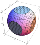
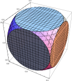
Figure 1: State space for noisy Bell measurement for $\lambda=1/4$ (left) and $\lambda=1/2$ (right).

Non-maximally entangled measurement. Here we take non-maximally entangled basis parametrized by $a$ and $b$

$$\tilde{\phi}_{\pm}=\frac{1}{\sqrt{2}}(a|0\rangle|0\rangle\pm b|1\rangle|1\rangle)$$

$$\tilde{\psi}_{\pm}=\frac{1}{\sqrt{2}}(a|0\rangle|1\rangle\pm b|1\rangle|0\rangle).$$ (18)

Taking $a=0,b=1$ leads to product basis and $a=b=1/\sqrt{2}$ to standard Bell basis.

We express positivity conditions in terms of formula (10) (outcome $0$ refers to $\tilde{\phi}_{+}$, $1$ to $\tilde{\phi}_{-}$, etc.):

$$T_{1} = \frac{1}{4}\left(\begin{array}[]{cccc}2ab&0&0&0\\ 0&-2ab&0&0\\ 0&0&1&a^{2}-b^{2}\\ 0&0&a^{2}-b^{2}&1\end{array}\right),$$ (23)

$$T_{2} = \frac{1}{4}\left(\begin{array}[]{cccc}-2ab&0&0&0\\ 0&2ab&0&0\\ 0&0&1&a^{2}-b^{2}\\ 0&0&a^{2}-b^{2}&1\end{array}\right),$$ (28)

$$T_{3} = \frac{1}{4}\left(\begin{array}[]{cccc}2ab&0&0&0\\ 0&2ab&0&0\\ 0&0&-1&a^{2}-b^{2}\\ 0&0&-a^{2}+b^{2}&1\end{array}\right),$$ (33)

$$T_{4} = \frac{1}{4}\left(\begin{array}[]{cccc}-2ab&0&0&0\\ 0&-2ab&0&0\\ 0&0&-1&a^{2}-b^{2}\\ 0&0&-a^{2}+b^{2}&1\end{array}\right).$$ (38)

In the following part we will analyze state space for particular basis with $a=\sin(\pi/4+\alpha)$, $b=\cos(\pi/4+\alpha)$. For that parametrization we can write (10) as (cf. (12)-(15)):

$$-m^{A}_{Z}m^{B}_{Z}+(-m^{A}_{X}m^{B}_{X}+m^{A}_{Y}m^{B}_{Y})\cos(2\alpha)$$

$$-(m^{A}_{Z}+m^{B}_{Z})\sin(2\alpha) \leq 1,$$

$$-m^{A}_{Z}m^{B}_{Z}+(m^{A}_{X}m^{B}_{X}-m^{A}_{Y}m^{B}_{Y})\cos(2\alpha)$$

$$+(m^{A}_{Z}+m^{B}_{Z})\sin(2\alpha) \leq 1,$$

$$m^{A}_{Z}m^{B}_{Z}-(m^{A}_{X}m^{B}_{X}+m^{A}_{Y}m^{B}_{Y})\cos(2\alpha)$$

$$-(m^{A}_{Z}-m^{B}_{Z})\sin(2\alpha) \leq 1,$$

$$m^{A}_{Z}m^{B}_{Z}+(m^{A}_{X}m^{B}_{X}+m^{A}_{Y}m^{B}_{Y})\cos(2\alpha)$$

$$+(m^{A}_{Z}-m^{B}_{Z})\sin(2\alpha) \leq 1.$$

It is hard to obtain full state space for given positivity conditions. Moreover there may be many inequivalent states spaces. Here we are interested in interpolation between quantum and unrestricted system. For this reason we bound state space of single system from inside by cube in moments representation with vertices $(\pm l,\pm l,\pm h)$. Because of linearity it is enough to check if vertices fulfill positivity conditions. For Bell basis ($\alpha=0$ which leads to $a=b=1/\sqrt{2}$) we get condition:

$$2l^{2}+h^{2}\leq 1.$$ (39)

On FIG. 2 we present permitted values of $l$ and $h$ for different parameter $\alpha$.

Figure 2: Allowed values of $l$ (OY) and $h$ (OX) for $\alpha=\pi/16,2\pi/16,3\pi/16,4\pi/16$. Thick black line bounds region permitted in quantum mechanics. We can observe interpolation between quantum and unrestricted system.

VI Concluding remarks

Our model of no-signaling boxes admitting Bell measurement or non-maximally entangled measurement is just an example of constraining the nosignaling theory by amending it by quantum-inherited joint measurements. The results encourage to study other amendments, and checking their properties. In particular, it is worth to examine multipartite systems where quantumness of local systems does not determine the correlations anymore tripartite_local_quantum . Another route is to consider more general parity measurements, e.g with more outcomes than just four, in place of Bell measurements. Finally it would be interesting to perform more detailed study of the correlations exhibited by no-signaling systems with non-maximally entangled measurements. Such analysis involves a highly nonlinear problem, which requires further investigations.

Acknowledgements. ŁCz and MH are supported by John Templeton Foundation.

References

- (1) S. Popescu and D. Rohrlich, Found. Phys. 24, 379 (1994).
- (2) G. Mackey, Mathematical Foundations of Quantum Mechanics, Benjamin, 1963.
- (3) E. B. Davies, J. T. Lewis, An operational approach to quantum probability, Comm. Math. Phys. 17 (1970) 239-260
- (4) C. M. Edwards, The operational approach to quantum probability I, Comm. Math. Phys. 17 (1971), 207-230.
- (5) S. L. Braunstein, A. Mann and M. Revzen , Phys. Rev. Lett. 68, 3259 (1992).
- (6) J. Barrett, N. Linden, S. Massar, S. Pironio, S. Popescu, and D. Roberts, PRA 71, 022101 (2005), arXiv:quantph/0404097.
- (7) J. Barrett, L. Hardy, A. Kent, No signaling and quantum key distribution. Phys. Rev. Lett. 95, 010503 (2005).
- (8) Pironio, S. et al., Random numbers certified by Bell’s theorem. Nature 464, 1021–1024 (2010).
- (9) R. Colbeck and R. Renner, Free randomness can be amplified. Nat. Phys. 8, 450–454 (2012)
- (10) N. Brunner, D. Cavalcanti, S. Pironio, V. Scarani, S. Wehner, Bell nonlocality, Rev. Mod. Phys. 86, 419 (2014), arXiv:1303.2849
- (11) T. Tylec and M. Kuś, J. Phys. A: Math. Theor. 48 (2015) 505303.
- (12) H. Barnum, S. Beigi, S. Boixo, M. B. Elliott, S. Wehner, Local Quantum Measurement and No-Signaling Imply Quantum Correlations Phys. Rev. Lett. 104, 140401 (2010)
- (13) M. Dall’Arno, S. Brandsen, A. Tosini, F. Buscemi, V. Vedral No-hypersignaling principle, Phys. Rev. Lett. 119, 020401 (2017)
- (14) B. S. Cirel’son, Quantum generalizations of Bell’s inequality. Letters in Mathematical Physics, 4, 93–100 (1980)
- (15) S. Massar, M.K. Patra, Information and communication in polygon theories, Phys. Rev. A 89, 052124 (2014), arXiv:1403.2509 (2014).
- (16) P. Janotta, C. Gogolin, J. Barrett, N. Brunner, Limits on non-local correlations from the structure of the local state space New J. Phys. 13, 063024 (2011), arXiv:1012.1215.
- (17) H. Barnum, J. Barrett, M. Leifer, A. Wilce, Teleportation in General Probabilistic Theories, arXiv:0805.3553 (2008)
- (18) P. Janotta, H. Hinrichsen, Generalized Probability Theories: What determines the structure of quantum theory? J. Phys. A: Math. Theor. 47, 323001 (2014)
- (19) M. Kliiy, C. Randall, and D. Foulis, Tensor Products and Probability Weights, Int. J. of Th. Phys. 26, 199 (1987).
- (20) H. Barnum, C. A. Fuchs, J. M. Renes, A. Wilce, Influence-free states on compound quantum systems, arXiv:quant-ph/0507108 (2005).
- (21) S. L. Woronowicz, Positive maps of low dimensional matrix algebras, Rep. Math. Phys. 10, 165 (1976)
- (22) H. Araki, On a characterization of the state space of quantum mechanics, Comm. Math. Phys. 75 (1980), 1-24.
- (23) H. Barnum, A. Wilce, Local Tomography and the Jordan Structure of Quantum Theory, Found Phys 44, 192 (2014)
- (24) L. Hardy, W.K. Wootters, Limited Holism and RealVector-Space Quantum Theory, Found. Phys. 42, 454 (2012)
- (25) A. Acin, R. Augusiak, D. Cavalcanti, C. Hadley, J. K. Korbicz, M. Lewenstein, Ll. Masanes, M. Piani Unified Framework for Correlations in Terms of Local Quantum Observables, Phys. Rev. Lett. 104, 140404 (2010)