2 Departamento de Astrofísica, Universidad de La Laguna, E-38206 La Laguna, Tenerife, Spain
Impact of young stellar components on quiescent galaxies: deconstructing cosmic chronometers
Abstract
Context. Cosmic chronometers may be used to measure the age difference between passively evolving galaxy populations to calculate the Hubble parameter as a function of redshift . The age estimator emerges from the relationship between the amplitude of the rest frame Balmer break at 4000 Å and the age of a galaxy, assuming that there is one single stellar population within each galaxy.
Aims. First, we analyze the effect on the age estimates from the possible contamination (% of the stellar mass in our high-redshift sample) of a young component of Myr embedded within the predominantly old population of the quiescent galaxy. Recent literature has shown this combination to be present in very massive passively evolving galaxies. Second, we evaluate how the available data compare with the predictions of nine different cosmological models.
Methods. For the first task, we calculated the average flux contamination due to a young component in the Balmer break from the data of 20 galaxies at that included photometry from the far-ultraviolet to near-infrared at rest. For the second task, we compared the data with the predictions of each model, using a new approach of distinguishing between systematic and statistical errors. In previous work with cosmic chronometers, these have simply been added in quadrature. We also evaluated the effects of contamination by a young stellar component.
Results. The ages inferred using cosmic chronometers represent a galaxy-wide average rather than a characteristic of the oldest population alone. The average contribution from the young component to the rest luminosity at 4000 Å may constitute a third of the luminosity in some samples, which means that this is far from negligible. This ratio is significantly dependent on stellar mass, proportional to . Consequently, the measurements of the absolute value of the age or the differential age between different redshifts are at least partially incorrect and make the calculation of very inaccurate. Some cosmological models, such as the Einstein-de Sitter model or quasi-steady state cosmology, which are rejected under the assumption of a purely old population, can be made compatible with the predicted ages of the Universe as a function of redshift if we take this contamination into account. However, the static Universe models are rejected by these measurements, even when this contamination is taken into account.
Key Words.:
Galaxies: evolution – Galaxies: high-redshift – Cosmology: observations1 Introduction
The geometry of the Universe and the reality of its expansion may be tested by means of various analyses of the galaxy distribution, either in space or in time. The task is not simple and straightforward because there are many selection effects that mix truly cosmological effects with the evolution of galaxies, redshift distortions, and other influences, thus limiting the capability of the tests to constrain cosmological models without strong systematic effects (see, e.g., Baryshev & Teerikorpi 2012; López-Corredoira 2017).
For the time measurements, cosmological models provide precise predictions of the age of the Universe at a given distance, thus allowing a comparison with any chronometric measurements that establish how fast time changes with redshift. An example of an attempt to constrain cosmological models with this type of time measurement is the derivation of the Hubble parameter as a function of redshift (Jiménez & Loeb 2002; Moresco et al. 2012, 2016; Ratsimbazafy et al. 2017), using massive (with a stellar content M⊙), passively evolving galaxies; this method is called “cosmic chronometers”. This technique uses the age difference between passively evolving galaxies at different redshifts to calculate the expansion rate of the Universe. In addition to its use as a tool for constraining the cosmological parameters in the standard model, it has also been used to successfully fit the data with the predictions of other competing alternative models, such as the Universe (Melia & Maier 2013; Melia & McClintock 2015; Wei et al. 2017; Leaf & Melia 2017; Melia & Yennapureddy 2018).
We here extend the way different cosmologies are tested using this method in several important ways. We begin with a discussion of the misconceptions concerning this method, both in terms of the a priori assumption of a single stellar population (§2), and in the handling of the statistical and systematic errors in the analysis (§3). We carry out a comparative analysis of nine different models in §4 and dedicate a final section (§5) to the conclusions and further discussion.
2 Critical assessment of the measurements
The main flaw of the cosmic chronometer method is that it assumes that early-type galaxies have only a single burst stellar population (SSP) or an extended stellar star formation with a very fast decay (star formation ratio with Gyr), which is in practice comparable to a Dirac’s delta in the distribution of ages of an SSP, especially when observed in the nearby Universe. Observational evidence suggests that this assumption is not valid, given that one SSP cannot fully describe early-type galaxies in general at any redshift and any stellar mass (Burstein et al. 1988; Vazdekis et al. 1997, 2016; Yi et al. 2007, 2011; Atlee et al. 2009; Salim & Rich 2010; Mok et al. 2014; López-Corredoira et al. 2017 [hereafter L17]), and because there is residual gas even at high-redshift quiescent galaxies (Concas et al. 2017; Gobat et al. 2017). It is relevant that this young population for the most massive galaxies affects the samples used for cosmic chronometers. Specifically, fits to the galaxy spectra based on one SSP do not provide consistent results for the blue and red wavelengths at high redshifts; at least two SSPs are necessary to match the photometric and spectroscopic data, with the bulk of the stellar population being very old and the remaining contribution coming from a young component that is due to residual star formation (Oser et al. 2010). The evidence of this second young burst arises because the UV spectral range is almost unnoticed in the visible. This “contamination” represents a drawback with age estimator methods that are based on single lines or breaks, such as the Balmer break used in cosmic chronometers, thus (perhaps severely) weakening the application of this technique to constrain cosmological parameters.
L17 demonstrated that some age-sensitive breaks, such as the Balmer break at 4 000 Å at rest, have contributions from significant fractions of light of two such components, therefore they cannot serve as a simple, direct indicator of the age of the oldest population, but instead represent a luminosity-weighted age of the young and the old populations. One might think that such double populations affect only a few quiescent galaxies and that most of them are reasonably well fit with only one SSP. However, observational evidence to support this is lacking; quite to the contrary, photometry in the wavelength of the far UV at rest is needed to characterize the young component, and this is not done in most of the quiescent galaxies at low-intermediate redshifts, which are typically observed only in the visible. In the few cases where UV photometry at rest is available, a V-shaped pattern with a minimum flux around the wavelength at rest of 3000 Å is observed (e.g., Yi et al. 2011, middle panel of Fig. 3), characteristic of a two-component synthesis. The analysis of Yi et al. (2011) with SDSS-GALEX galaxies showed that 30-40% of the galaxies have a conspicuous V-shape, which is the signal of a young component similar to what was observed in the sample of L17 at high redshift: see Fig. 1. The Balmer break is correlated with the (far UV)-r color (Rich et al. 2005, middle panel of Fig. 2), which also indicates that the higher the young component contamination (the lower the (far UV)-r color), the lower the average age (the lower the Balmer break). Therefore, the claim of a pure single stellar population cannot be supported in general.
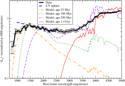
There are other possibilities to explain the UV excesses that do not include a young component, such as a UV upturn, defined as rising flux with decreasing wavelength from about 2500 Å to 1000 Å (e.g., Bertola et al. 1982; Yi et al. 2011; Boissier et al. 2018). The UV upturn was found in the nearby Universe in quiescent galaxies and has originally been associated with the production of very hot stars by a young stellar population (O’Connell 1999), but it has also been associated with old stellar systems (Ferguson 1999, Brown 2004) such as old open (Buzzoni et al. 2012) and globular cluster environments (Perina et al. 2011). Several theoretical works studied the excess UV emission of various types of stars during their advanced evolutionary phases (Greggio & Renzini 1990; D’Cruz et al. 1996), although stellar evolution alone cannot provide a full explanation of the UV upturn (Greggio & Renzini 1990). Explanations were given in terms of extremely horizontal branch stars, in which low-mass helium-burning stars have lost their hydrogen-rich envelope (Brown 2004; Han et al. 2007), or the effect of binarity, with stars losing their hydrogen envelopes during binary interactions (Han et al. 2007; Hernández-Pérez & Bruzual 2014). Yi et al. (2011) also considered the UV upturn phenomenon in quiescent galaxies. They showed that 5% of their sample (within SDSS-GALEX low-z elliptical galaxies in clusters) show a UV upturn and 27% of them have residual star formation, which means that although the UV upturn may be another effect to take into account, it is not the dominant one in their sample. Similarly, the UV upturn, regardless of its origin, is not the dominant contribution in the spectral range aroung 2000-2500 Å. Fig. 1 shows that a young stellar component fits the average luminosites at rest in the L17 sample, whereas a UV upturn (merely with a linear or almost-linear , as has commonly been fit by other authors; e.g., Yi et al. 2011, top panel in Fig. 3; Boissier et al. 2018, top panel in Fig. 1) does not because the UV luminosity decreases below 1500 Å. There is a clear bump in the UV regime, expected in the presence of a young population of Myr, but not for the UV upturn. The models that use an almost linear below 1500 Å might be missing some deeper effect of the Lyman break, but even so, a functional shape as observed in Fig. 1 may not be reproduced in these terms. Therefore, even if we admit that some galaxies might present a UV upturn as well, we consider that it is not enough to explain the observed UV features. However, a fit with two SSPs can even explain the UV upturn in the few galaxies that present that feature with a very young population ( 25 Myr; L17), therefore we keep the two-SSP model as a valid way to fit the spectrophotometry of the galaxies and do not consider any further effect of possible old populations with binarity effects, hot horizontal branch, post-AGB, or others (stellar populations with ages Gyr are excluded given the high redshift of our sample). To summarize, we do not discard the possibility that there might be some effect from the old populations in UV excess, but we consider that at least some amount of young population is necessary. Therefore, estimates for the amount of the young contribution represent an approximate maximum limit.
The cosmic chronometer method measures the differential age as a function of redshift. The Hubble parameter may be calculated as , from which one may infer that (Moresco et al. 2012, 2016)
| (1) |
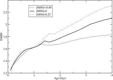
where the Balmer break . This may be approached as with one SSP, , . This is only a very rough approximation because, as Fig. 2 shows, the dependence of the Balmer break on age is not linear in the young-age regime. Nonetheless, this expression is commonly used with the cosmic chronometer method (indeed, it is used only for old ages, with and with two linear regimes instead of one; Moresco et al. 2012). For instance, from a fit to Fig. 2 for solar metallicity, the values of a linear fit in the regime between 1 and 4 Gyr would give Gyr-1, . With a double component of young+old stars with respective ages age1 and age2 Gyr, however, the combined Balmer break with the two populations is instead
| (2) |
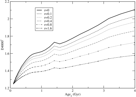
where , that is, the ratio of luminosities due to the young and old population for the Balmer break. If we use the measured without taking into account the contamination of the young population (see Figure 3), we obtain a large deviation with respect to the value of age2 for high values of . If we assume a linear variation of the young/old population such that , and a constant , the measured Hubble parameter is related to the true Hubble parameter by the expression
| (3) |
where
There are other indicators of age, such as the Hβ Lick index, but this was also shown to be affected by the possible presence of ionized gas even in the most massive and passive galaxies (Concas et al. 2017).
2.1 Ratio of luminosities in a high-redshift sample
L17 fit the spectra of 20 very massive ( M⊙) quiescent galaxies at high redshift using two such populations with ages of age Gyr (young) and age Gyr (old; weighted average, error: 0.5 Gyr). The Balmer break assuming solar metallicity would be and 1.72 for the younger and older populations, respectively, using the E-MILES synthesis population model (Vazdekis et al. 2016); see Fig. 2. The average ratio in this sample is , with an r.m.s. . Hence, the average Balmer break is , corresponding to an average age Gyr (using the E-MILES model; see Fig. 2), almost independently of the metallicity. This means that using the Balmer break in these cases and assuming a single population, the age of the galaxy is underestimated. An average Gyr would be measured instead of the true age of the oldest population, which is equal to 1.5 Gyr.
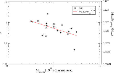
This sample shows some dependence on stellar mass. In Fig. 4 we show the ratio versus an estimated stellar mass of the sample in L17. In the calculation of the stellar mass, we neglected the mass of the young stars, assumed the age of the old population in all of the galaxies to be 1.5 Gyr, and compared it with the stellar population synthesis E-MILES model (Vazdekis et al. 2016). The best power-law fit gives . This is a significant mass dependence, which agrees with the results by Caldwell et al. (2003), who found that low-velocity dispersion galaxies have younger mean ages. In cosmic chronometer samples, the samples are constrained to have M⊙, which means that on average.
The impact of a young component ( Gyr) with luminosity at 4000 Å equal to 50% of the luminosity at the wavelength of an older population (1.5 Gyr) is plausible and not surprising. The mass/luminosity ratio at this wavelength is times higher for the older population of 1.5 Gyr than for stars with an age Gyr (using the E-MILES stellar population synthesis model, assuming solar metallicity and a Kroupa universal IMF; Vazdekis et al. 2016). Therefore, the young population can indeed significantly contaminate the spectrum while still representing only of the stellar mass. This is compatible with the fact that the galaxies are elliptical and dominated in mass by an older population, consistent with what is observed in other nearby galaxies (e.g., Yi et al. 2011; Vazdekis et al. 2016). Note that this young component might be associated with the gas budget remaining after the main star formation episode that took place 1.5 Gyr earlier, which led to the formation of the vast majority of the stellar populations of the galaxy. In the nearby Universe, this scenario is consistent with a dominant stellar population evolving passively that hosts some residual in situ star formation, as observed in local galaxies. Therefore the young component obtained in L17 by means of the two-SSP approach should be regarded as a mean luminosity–weighted contribution that is representative of the most recent tail that extends in time after reaching the peak of star formation.
A mean amount of % of the stellar mass in galaxies with total stellar mass of M⊙ means M⊙ of young stars, which implies that M⊙, so that the mean star formation rate is . The time extent in which the star formation took place, , would be Myr if the 100 Myr contribution represented an average of constant [SFR]. However, since the age obtained for the young burst in the two-SSP approach is in reality a mean luminosity-weighted age, this contribution has to be associated with an even longer star formation period as the youngest bursts are far more luminous in the UV, thus biasing our solution toward a younger SSP. An exponentially decaying star formation model (L17, sect. 6) gives the best fit for [SFR] almost constant () (although this is not as good as the two-SSP solution). Therefore, the box of integration corresponding to the ages of the young population might be extended up to high intermediate ages. The youngest end has the greatest effect because of the strong emission in UV, and the oldest component ( Gyr) because of its overwhelming contribution in mass; the intermediate ages might be present in the galaxies as well, but they provide a relatively far lower contribution because of the low mass. The 100 Myr like SSP has to be understood as a mean luminosity-weighted contribution of a young population with an age Gyr. This suggest that the mass of the young population is formed during several hundreds of Myr. Therefore, is larger than 200 Myr and the mean is M⊙/yr. In our sample, there is no detectable strong star formation, as we do not see strong emission lines (see spectra in L17 for two of these galaxies), as they were photometrically selected to be quiescent galaxies, and the galaxies were required to have no significant emission at [24m], expected from dust associated with star formation (Castro-Rodríguez & López-Corredoira 2012). The SFR in the moment in which they were observed must therefore be very low in these galaxies. The possible episodes of star formation of the galaxy have occurred in epochs previous to the observation by several tens or hundreds of Myr, not in the moment in which the galaxies were observed. The SFR may have some fluctuations such that there are periods in which the galaxies have no significant observable star formation activity, and one such low SFR epochs must be the one in which the galaxies are observed.
In the subsample examined by L17 with an estimated stellar mass higher than M⊙, , with an r.m.s. of 0.22 (hence, the error of the mean is 0.07), if we assume non-variability of this ratio with redshift (), we could say that for each galaxy in this sample . That is, if we used the cosmic chronometer method in this subsample, the value of the Hubble parameter would be overestimated by some unknown factor between 1.25 and 1.69 within 1. We also note that this should represent a maximum limit in this high-redshift sample because possibly all of the UV contribution might not necessarily be attributed to a young stellar component and there may be other possible contributions associated with the UV upturn phenomenon (see the discussion of the UV upturn above). Therefore, we should adopt and .
We can also perform a double power-law fit with the data using , for which the result is , with a slightly significant negative ; in this case, , and . In either case, this large dispersion of systematic deviations does not allow us to compare measurements with the predictions of various cosmological models.
This may represent a very pessimistic scenario with a very high contamination of young stars. The samples used in the application of cosmic chronometer methods may be less strongly contaminated, but we do not know the value of for these samples because there are no fits using UV photometry in them.
3 Statistical analysis to fit cosmological models
The comparison of the measured with the predictions of different cosmological models necessarily involves two important aspects: 1) the combination of statistical and systematic errors, and 2) the inclusion of other published values of derived using different methods.
3.1 Combining statistical and systematic errors
Most workers in the field, such as Moresco et al. (2012, 2016), simply added statistical and systematic errors in quadrature. The justification is based on the view that differential dating removes constant systematic uncertainties, so that the residuals are uncorrelated. The systematic errors published with the measurements, however, include an estimate of stellar metallicity that is measured independently in each redshift bin. Although this might provide uncorrelated and independent measurements in principle, they are nonetheless at least partially correlated. At best, one can view these systematic errors as having some component that one may add in quadrature with statistical errors, but not the correlated parts. One way to show that the systematic errors cannot be entirely uncorrelated is that the total error resulting from addition in quadrature is too large compared with the deviations of the data relative to any of the best-fit models (see, e.g., Moresco et al. 2016, Fig. 6; Melia & Maier 2013; Melia & Yennapureddy 2018). These errors produce a reduced chi-square that is significantly smaller than one. Moreover, Leaf & Melia (2017) have shown that the global errors of measurements are not Gaussian, therefore they cannot be purely statistical.
A more appropriate method of combining statistical errors with systematic errors that are only partially uncorrelated would be the following (Melia & Yennapureddy 2018):
| (4) |
| (5) |
where is an unknown constant that represents the degree of uncorrelation in the systematic errors. For , the systematic errors are completely correlated, whereas for , the systematic errors are totally random and can be added with the statistical errors in quadrature. We assume here that does not depend on redshift. However, this unknown quantity cannot be calculated directly, although we can fit in order to ensure that the optimized fit of the best model has .
Now, even if we knew the true systematic error and the true statistical error , the method for testing cosmological models cannot be based solely on summing them quadratically and then minimizing , or maximizing the likelihood function. This is typically done in cosmology, based on a misconception in the statistical analysis, but it is not a correct approach. Cosmologists often show merit functions with contours representing the confidence regions that constrain the optimized parameters, but systematic errors cannot be included in this manner. There is no way to calculate the error bars of a parameter in a model when we have both statistical and systematic uncertainties. At best, we can only tell whether a given model with certain parameter values is compatible with the data, but no confidence level in the merit functions can be plotted. In other words, we cannot treat systematic errors as if they were uncorrelated and Gaussian.
One possible way to combine the different errors in is to carry out the fitting by generating a family of solutions , with all values in the range and assigning to each a statistical error . We here assume that the deviation of with respect to the measured is in the same direction as, and by the same ratio of, the systematic error. Of course, this prescription is not unique, but it is a much better approach than simply summing the statistical and systematic errors in quadrature. We use this approach to fit the cosmological models for each using, for instance, the minimization of , or the maximization of the likelihood function, and we choose the value of corresponding to the smallest of the minima in (or the largest of the maxima if we use the likelihood function). The probability associated with the smallest of the minima in gives us the maximum probability, , of the model to fit the data.
3.2 Locally measured values of
Another problem with the use of cosmic chronometers for measuring is the inclusion of derived with other data, such as Type 1a supernovae (SNe) at . This should not be done because the calibration used for cosmic chronometers is subject to different systematics than those of other methods (Wei et al. 2017). Furthermore, is an amplitude for all the measurements using cosmic chronometers, and is not an independent datum. It should be treated as a free parameter in a fit, while the introduction of an a priori value for it produces deviations with respect to the rest of the global fit based solely on cosmic chronometer data. Wei et al. (2017 and references therein) argued that a local measurement of would not be the same as that derived for the background if the local expansion rate were influenced by a Hubble bubble.
Surprisingly, the value of in the lowest bins obtained from cosmic chronometers is very close to the value obtained by the cosmological groups using Cosmic Microwave Background Radiation (CMBR), gravitational lensing, or SNe. For instance, the value of km s-1 Mpc-1 by Moresco et al. (2012) using galaxies of the SDSS survey and the Bruzual & Charlot (2003, hereafter BC03) synthesis model. Assuming standard cosmology with , this would imply a calibration of (syst.) km s-1 Mpc-1, which is very close to the values of km s-1 Mpc-1 from SNe data (Riess et al. 2016) or km s-1 Mpc-1 from CMBR (of the Planck mission) and lensing data (Planck Collaboration 2016). In addition to the recognized fact that SNe measurements and CMBR measurements differ, we may admire here that the cosmic chronometer value of is also quite accurate and compatible with other cosmological measurements. The fact that they get with high accuracy implies that 1) either and (no evolution of the ratio ), that is, no contamination of a young component (), because for a non-evolving case of constant , (from Eq. 3); or 2) evolves (), and then can be obtained with the constraint (assuming , , km s-1Mpc-1=0.070 Gyr-1, Gyr-1 (Moresco et al. 2012, model BC03, solar metallicity, high )). We know that condition 1) cannot be true, Moresco et al. cannot avoid within such low values of the possible contamination of young population using only SDSS data, without UV spectra. We repeat that Yi et al. (2011) demonstrated that the contamination of residual young components is also important in SDSS quiescent galaxies at low . The coincidence that we obtain the same value of as other cosmological groups might be due to a coincidence by which is significantly larger than 0 and , or to the fact that there are other systematic errors that compensate for the effect of a young component (). Therefore, the calibration of this should be taken with a grain of salt.
| Model | Free cosmol. parameters | |
|---|---|---|
| CDM, standard | ||
| CDM, free | , | |
| CDM | , , | |
| Einstein-de Sitter | ||
| Friedmann open | , | |
| QSSC | , , | |
| and Milne | ||
| Static, linear Hubble law | ||
| Static, tired light |
3.3 Model selection statistics
The minimum deviation between a model and data is obtained when the is a minimum. Nonetheless, in order to compare the likelihood of different models with different numbers of free parameters, we also need to evaluate the effect of adding free parameters to reduce the . Unfortunately, there is no universal approach to accurately estimating the probability of a cosmology fitting the data using a single formula for penalizing the less parsimonious models. Nonetheless, we can calculate a range of probabilities by surveying the results of several representative methods that punish the excessive use of free parameters using various criteria. In general, all these approaches agree that the model most likely to be correct is the one with a minimum value of
| (6) |
where is the number of free parameters, and is a constant that depends on the statistical method.
For the most common version of the minimization of the reduced chi-square: , for a large number of data points . Hence, , . That is, the minimum value of is around one for a good fit (). In our case, as we show below, some cosmological models do not produce good fits (), but this is for cases without an increase in free cosmological parameters except for and , so that they are not affected by the deviations of this approximation.
It is now common in cosmology to compare the evidence for and against competing models using the information criteria (IC; for some of the earliest applications, see, e.g., Takeuchi 2000; Liddle 2004, 2007; Tan & Biswas 2012; Melia & Maier 2013). These criteria constitute an enhanced goodness of fit that extends the usual criterion by more fairly taking into account the number of free parameters in each model. These tools prefer the more parsimonious models, unless the introduction of an additional parameter provides a substantially better fit to the data. This approach reduces the possibility of overfitting, that is to say, an outcome in which optimizing with a greater number of free parameters simply fits the noise. These criteria yield the relative ranking of two or more competing models, along with a numerical assessment of the confidence that each model is the best, analogous to likelihoods or posterior probabilities in conventional statistical inference. Unlike the latter, however, the IC methods can be applied to models that are not ‘nested,’ that is, models that are not specializations of each other.
One of the oldest IC methods, known as the Akaike information criterion (AIC; Akaike 1973; see also Burnham & Anderson 2002, 2004), provides the relative ranks of two or more competing models, and also a numerical measure of confidence that each model is the best. These confidences are analogous to likelihoods or posterior probabilities in traditional statistical inference. With this method, the quantity is minimized (see, e.g., Melia & Meier 2013, Eq. 5), so that .
Other methods have subsequently been developed based on IC, including the Kullback information criterion (KIC; Cavanaugh 2004) and the Bayesian information criterion (BIC; Schwarz 1978). KIC and BIC are symmetrized versions of the probability density functions of the “true” model and the model being tested (Cavanaugh 1999), whereas AIC does not symmetrize them. For KIC, , a value based on a derivation in information theory with close ties to statistical mechanics (see also Bhansali & Downham 1977). The corresponding BIC has , where is the number of data points. This is a misnomer because it is not really based on information theory; it is instead an asymptotic () approximation to the outcome of a conventional Bayesian inference procedure for deciding between models (Schwarz 1978). Tests have shown that the BIC outperforms other such criteria used in model selection when the sample is very large (see, e.g., Liddle 2004, 2007). In this paper, we have 17 data points, for which is close to .
In a comparison of two or more competing models, , the model with the smallest is assessed to be the model nearest to the ‘truth,’ that is, to the actual correct (although perhaps still) unknown model that produced the data. More quantitatively, the models may be ranked as follows. If model has , the non-normalized likelihood that is closest to the truth is the weight , with
| (7) |
of being closest to the correct model. In comparing a pair of models , the difference determines the extent to which is favored over . For , the evidence in favor of model is considered to be weak. The evidence is mildly in favor of for , and it is strong for .
4 Model selection
Moresco et al. (2012, 2016) have focused their use of cosmic chronometer data exclusively on the optimization of parameters in the standard model. We can broaden the applicability of these observations by comparing different cosmological models. We analyze and compare the models listed in Table 1, along with their individual predictions for . Melia & Yennapureddy (2018) also tried to compare these data with some of these cosmological models, but they restricted their comparison to the CDM/CDM model with only one free parameter (including ), whereas here we leave more unrestricted possibilities of fitting the model with different cosmological parameters. We fit a CDM cosmological model with either 1 (), 2 (, ) or 3 (, and the equation of state for dark energy ) free cosmological parameters. Two settings are valid: either leaving , as free parameters or taking them fixed within the “standard” values to check that this model with these parameters does reproduce the data of cosmic chronometers; and the effect of including a higher number of free parameters is taken into account with the method explained in §3.3. We assume, however, that is constant, equal to unity, and do not let this parameter vary. We note that for all the expanding models, that is, for all models but the last two, .
4.1 Data
We focus on the 17 measurements of taken from the literature that have a published separation of the statistical and systematic errors. These values are listed in Table 2. We caution, however, that these systematic errors do not include the progenitor bias, as they are considered negligible with respect to other uncertainties (Moresco et al. 2012, 2016).
| Reference | ||||
|---|---|---|---|---|
| 0.179 | 75.0 | 3.8 | 0.5 | Moresco et al. (2012)/BC03 |
| 0.199 | 75.0 | 4.9 | 0.6 | Moresco et al. (2012)/BC03 |
| 0.240 | 79.7 | 2.3 | 1.3 | Gaztañaga et al. (2009) |
| 0.352 | 83.0 | 13.0 | 4.8 | Moresco et al. (2012)/BC03 |
| 0.380 | 83.0 | 4.3 | 12.9 | Moresco et al. (2016) |
| 0.400 | 77.0 | 2.1 | 10.0 | Moresco et al. (2016) |
| 0.420 | 86.4 | 3.3 | 1.7 | Gaztañaga et al. (2009) |
| 0.425 | 87.1 | 2.4 | 11.0 | Moresco et al. (2016) |
| 0.450 | 92.8 | 4.5 | 12.1 | Moresco et al. (2016) |
| 0.478 | 80.9 | 2.1 | 8.8 | Moresco et al. (2016) |
| 0.593 | 104.0 | 11.6 | 4.5 | Moresco et al. (2012)/BC03 |
| 0.680 | 92.0 | 6.4 | 4.3 | Moresco et al. (2012)/BC03 |
| 0.781 | 105.0 | 9.4 | 6.1 | Moresco et al. (2012)/BC03 |
| 0.875 | 125.0 | 15.3 | 6.0 | Moresco et al. (2012)/BC03 |
| 1.037 | 154.0 | 13.6 | 14.9 | Moresco et al. (2012)/BC03 |
| 1.363 | 160.0 | 22.1 | 24.0 | Moresco (2015, priv. comm.) |
| 1.965 | 186.5 | 40.9 | 28.0 | Moresco (2015, priv. comm.) |
| Model | Optimized free parameters | Probability range | |
|---|---|---|---|
| CDM, standard | , | 15.00-29.82 | 0.417-0.989 |
| CDM, free | , , | 14.84-31.38 | 0.295-0.953 |
| CDM | , , , | 13.42-26.29 | 0.0514-0.994 |
| and Milne | , | 18.50-39.00 | -0.733 |
| Friedmann open | , , | 18.43-40.09 | -0.331 |
| QSSC | , , , | 24.30-52.66 | -0.0235 |
| Einstein-de Sitter | , | 38.04-78.93 | - |
| Static, tired light | , | 58.51-106.19 | - |
| Static, linear Hubble law | , | 161.51-288.17 |
4.2 Assuming that the measurements of are correct
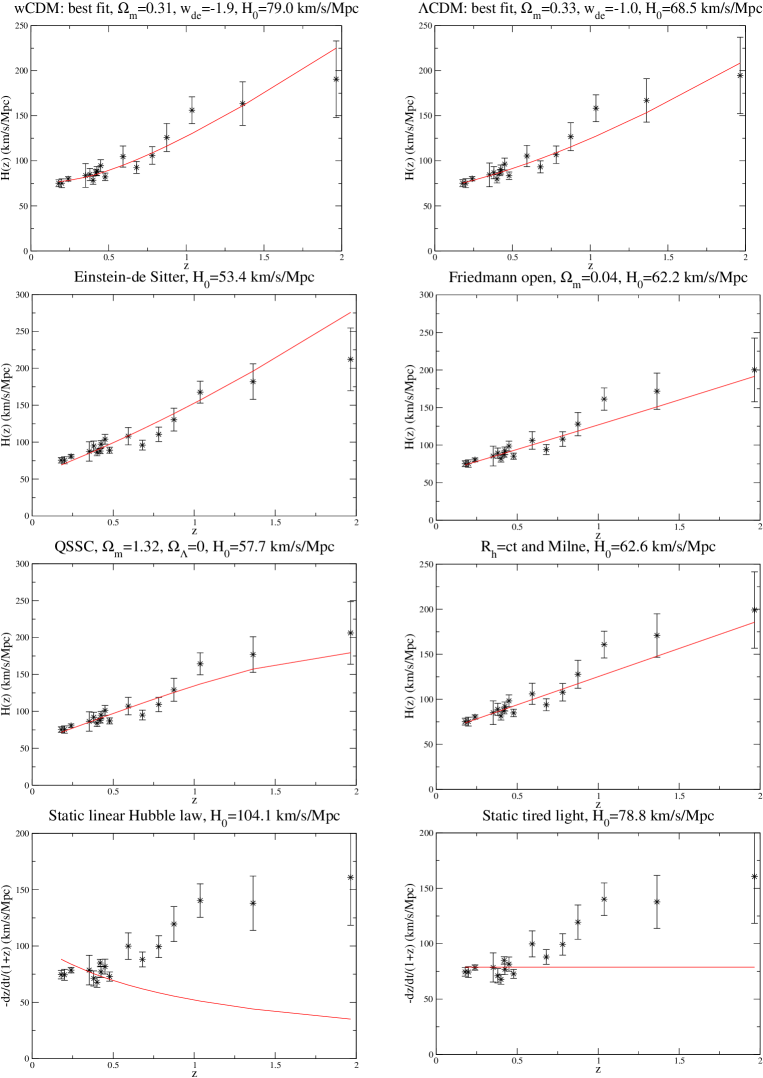
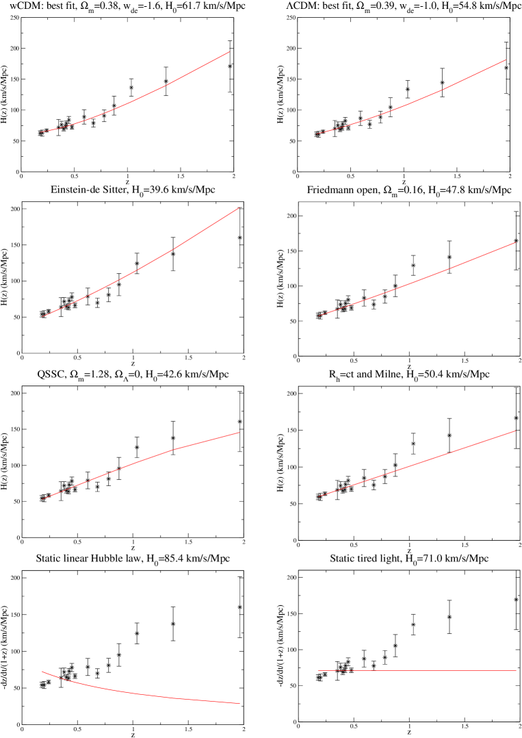
We first assume that in Equation (3), that is, that there is no contamination by a young stellar component and thus . We follow the procedure outlined in § 3.1. To estimate the fraction , we first fit the data with CDM and a fixed standard value of to obtain a (the number of free parameters here is two: and , so ). We obtain . The ranking of the various cosmological models was calculated relative to this optimization. The results of the fits for all the cosmologies are shown in Fig. 5 and listed in Table 3.
The optimized free parameters correspond to the best fits for the value of that minimizes . To calculate the errors, we used the standard test (Avni 1976) with the number of free parameters equal to the number the free cosmological parameters (1-3) plus one (i.e., ). The probabilities quoted in this table are calculated according to Equation (7), and their range includes the minimum and maximum values corresponding to between -1 and 1, between 1 and 3, for the three variants of the CDM/CDM model, and the assumption that only one of seven possibilities (there are seven possibilities in nine different cosmological models because Milne and have the same prediction, and wCDM and CDM do not exclude each other) may be correct. The favored model is the model CDM/CDM, except in the case of and three free cosmological parameters for this model, for which or Milne obtain a slightly higher probability for some values of . Previous claims of a better fit for model are based either on using only tests with the largest penalization on the large number of free parameters (Melia & Maier 2013; Melia & McClintock 2015; Wei et al. 2017) or using CDM/CDM allowing one free parameter at most, including (Melia & Yennapureddy 2018), which restricts the possibilities for exploring the full space of parameters in the standard cosmology. Here, we see that a global analysis with all possible model selection statistics and without restrictions a priori of some cosmological parameters favors the standard model over the model. There is also some support for the Friedmann open model. On the other hand, the quasi-steady state cosmology (QSSC) is rejected at % CL in every case. Other models, such as the Einstein-de Sitter model, the static tired light model, and static linear Hubble law cosmologies, are rejected very strongly. At this point, we have not yet taken into account the potentially large systematic errors that are due to contamination from young stars, as explained in § 2. We examine this effect next.
4.3 Effect on from the contamination of young stars
We now assume that the true Hubble parameter is related to the measured values given in Table 2 through Eq. (3), leaving the ratio (although constant in ) as a free parameter. The additional systematic error corresponding to this correction is .
| 0.136 | 0.113 | 0.075 | 0.034 | 0.0033 | ||
|---|---|---|---|---|---|---|
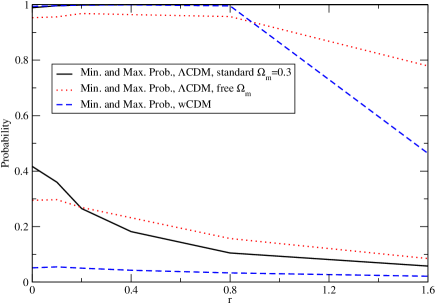
| Prob. [CDM, standard ] | 0.360-0.996 | 0.265-0.9986 | 0.182-0.99983 | 0.105-0.9999952 | 0.0578-1.000000 | |
| Prob. [CDM, free | 0.297-0.956 | 0.269-0.968 | 0.232-0.964 | 0.157-0.957 | 0.0849-0.779 | |
| Prob. [CDM] | 0.0549-0.996 | 0.0503-0.9983 | 0.0427- 0.99909 | 0.0331-0.9956 | 0.0212-0.464 | |
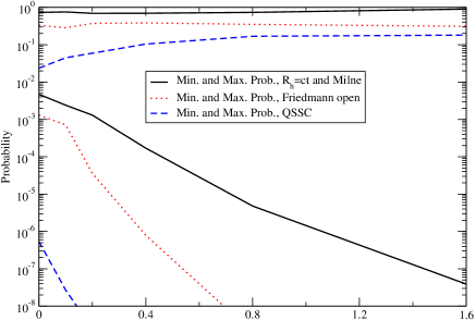
| Prob. [] or Prob.[Milne] | -0.753 | -0.691 | -0.695 | -0.733 | -0.899 | |
| Prob. [Friedmann open] | -0.284 | -0.372 | -0.384 | -0.350 | ||
| Prob. [QSSC] | -0.0447 | -0.0593 | -0.104 | -0.168 | ||
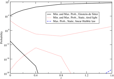
| Prob. [Einstein-de Sitter] | - | - | -0.0343 | |||
| Prob. [Static, tired light] | - | - | - | - | ||
| Prob. [Static, linear Hubble law] | 0 | 0 | 0 |
In Table 4 and Fig. 6 we quote the range of probabilities for and , based on the same criterion for the calculation of , that is, using as reference the best fit for the standard model without free parameters. In Fig. 7 we plot the best fits for the case of . The Einstein-de Sitter and QSSC models pass the test when we include this systematic error with an average value obtained in the analysis of L17 subsample with masses higher than M⊙. However, the two static models are rejected even for values as high as .
Although the cosmic chronometer method is not reliable enough to extract accurate cosmological information, we can therefore nonetheless use it to reject a static Universe at a very high confidence level. When the systematic error due to possible contamination by a young population is taken into account, however, the remaining models can pass the test.
5 Further discussion and conclusion
The cosmic chronometer method uses the age difference between a passively evolving population of galaxies at different redshifts to calculate the expansion rate of the Universe. This is an elegant way to derive cosmological information, provided that the age measurements reflect the time passed since the galaxy was formed. The proposers of this method use the relationship between the amplitude of the Balmer break at 4000 Å at rest and the age of the galaxy, including the possible effects of degeneracy with the metallicity, but what they measure is some kind of “average” age of the populations of the galaxy. The fact that there is a component of young stars in quiescent galaxies strongly contaminates the luminosity at the Balmer break wavelength, producing much lower values than the age of the oldest population in that galaxy.
As an example of this contamination, we have examined the sample of quiescent galaxies at with M⊙ in L17, which yield an average contribution to the luminosity at 4000 Å from the young component of about 50% of that due to the oldest population, that is, 33% of the total luminosity, which is far from negligible. This should be considered as an upper limit, as there might be other contributions from older stellar populations that might be associated with the UV upturn phenomenon, although our spectral energy distribution fitting points to a dominant contribution from the young component in this spectral range, most likely coming from the most recent tail of the main star formation event that took place 1 Gyr earlier. This ratio is significantly dependent on stellar mass, proportional to ; we will explore this important dependence in future works in more detail. The degree of contamination may vary in other samples of quiescent galaxies, but it is expected to be significant in all of them.
Consequently, measurements of the absolute value of the age, or the differential age between different redshifts, are incorrect, making the cosmic chronometer method very inaccurate. Even so, the predictions of by the various cosmological models are very different, and some exotic scenarios, such as the static Universe models, can be rejected.
Acknowledgements.
Thanks are given to F. Melia for his comments and suggestions to improve this paper, to J. Betancort-Rijo for some discussions on statistical techniques, to M. Moresco for clarifications of his papers and for providing the systematic errors of the points of Moresco (2015), to the anonymous referee for helpful comments, and to Astrid Peter (language editor of A&A) for the revision of this paper. MLC acknowledges support from grant AYA2015-66506-P from the Spanish Ministry of Economy and Competitiveness (MINECO). AV acknowledges support from grant AYA2016-77237-C3-1-P from the Spanish Ministry of Economy and Competitiveness (MINECO).References
- (1) Akaike, H., Petrov, B. N., Csáki F. 1973, Second International Symposium on Information Theory, Budapest Akadémiai Kiadó, p. 267
- (2) Atlee, D. W., Assef, R. J., & Kochanek, C. S. 2009, ApJ, 694, 1539
- (3) Avni, Y. 1976, ApJ, 210, 642
- (4) Baryshev, Yu. V., & Teerikorpi, P. 2012, Fundamental Questions of Practical Cosmology, Springer Verlag, Dordrecht
- (5) Bhansali, R. J. & Downham, D. Y. 1977, Biometrika, 64, 547
- (6) Bertola, F., Capaccioli, M., & Oke, J. B. 1982, ApJ, 254, 494
- (7) Boissier, S., Cucciati, O., Boselli, A., Mei, S., & Ferrarese, L. 2018, A&A, accepted [arXiv:1801.00985]
- (8) Brown, T. M. 2004, Ap&SS, 291, 215
- (9) Bruzual, G., & Charlot, S. 2003, MNRAS, 344, 1000 (BC03)
- (10) Burnham, K. P., & Anderson, D. R. 2002, Model Selection and Multimodel Inference (2nd edn.), Springer-Verlag, New York
- (11) Burstein, D., Bertola, F., Buson, L. M., Faber, S. M., & Lauer, T. R. 1988, ApJ, 328, 440
- (12) Buzzoni, A., Bertone, E., Carraro, G., & Buson, L. 2012, ApJ, 749, 35
- (13) Caldwell, N., Rose, J. A., Concannon, K. D. 2003, AJ, 125, 2891
- (14) Castro-Rodríguez, N., & López-Corredoira, M. 2012, A&A, 537, A31
- (15) Cavanaugh, J. E. 1999, Stat. Probab. Lett. 42, 333
- (16) Cavanaugh, J. E. 2004, Aust. N. Z. J. Stat., 46, 257
- (17) Concas, A., Pozzetti, L., Moresco, M., & Cimatti, A. 2017, arXiv:1702.07348
- (18) D’Cruz, N. L., Dorman, B., Rood, R. T., & O’Connell, R. W. 1996, ApJ, 466, 359
- (19) Ferguson, H. C. 1999, Ap&SS, 267, 263
- (20) Gaztañaga, E., Cabré, A., & Hui, L. 2009, MNRAS, 399, 1663
- (21) Gobat, R., Daddi, E., Magdis, G., et al. 2017, arXiv:1703.02207
- (22) Greggio, L., & Renzini, A. 1990, ApJ, 364, 35
- (23) Han, Z., Podsiadlowski, P., & Lynas-Gray, A. E. 2007, MNRAS, 380, 1098
- (24) Hernández-Pérez, F., & Bruzual, G. 2014, MNRAS, 444, 2571
- (25) Jiménez, R., & Loeb, A. 2002, ApJ, 573, 37
- (26) Leaf, K., & Melia, F. 2017, MNRAS, accepted [arXiv:1706.02116]
- (27) Liddle, A. R. 2004, MNRAS, 351, L49
- (28) Liddle, A. R. 2007, MNRAS, 377, L74
- (29) López-Corredoira, M. 2017, Foundations of Physics, 47, 711
- (30) López-Corredoira, M., Melia, F., Lusso, E., & Risaliti, G. 2016, IJMPD, 25, id. 1650060
- (31) López-Corredoira, M., Vazdekis, A., Gutiérrez, C. M., & Castro-Rodríguez, N. 2017, A&A, 600, A91 [L17]
- (32) Melia, F., & Maier, R. S. 2013, MNRAS, 432, 2669
- (33) Melia, F., & McClintock, T. M. 2015, AJ, 150, id. 119
- (34) Melia, F., & Yennapureddy, M. K. 2018, arXiv:1802.02255
- (35) Mok, A., Balogh, M. L., McGee, S. L., et al. 2014, MNRAS, 438, 3070
- (36) Moresco, M. 2015, MNRAS, 450, L16
- (37) Moresco, M., Cimatti, A., Jiménez, R., et al. 2012, JCAP, 8, id. 6
- (38) Moresco, M., Pozzetti, L., Cimatti, A., et al. 2016, JCAP, 5, id. 14
- (39) O’Connell, R. W. 1999, ARA&A, 37, 603
- (40) Oser, L., Ostriker, J. P., Naab, T., Johansson, P. H., & Burkert, A. 2010, ApJ, 725, 2312
- (41) Perina, S., Galleti, S., Fusi Pecci, F., Bellazzini, M., Federici, L., & Buzzoni, A. 2011, A&A, 531, A155
- (42) Planck Collaboration 2016, A&A, 594, A13
- (43) Ratsimbazafy, A. L., Loubser, S. I., Crawford, S. M., Cress, C. M., Bassett, B. A., Nichol, R. C., Väisänen, P. 2017, MNRAS, accepted. arXiv:1702.00418
- (44) Rich, E. M., Salim, S., Brinchmann, J., et al., 2005, ApJ, 619, L107
- (45) Riess, A. G., Macri, L. M., Hoffmann, S. L., et al. 2016, ApJ, 826, id. 56
- (46) Salim, S., & Rich, R. M. 2010, ApJ, 714, L290
- (47) Schwarz, G. 1978, Ann. Statist., 6, 461
- (48) Takeuchi, T. T. 2000, Ap&SS, 271, 213
- (49) Tan, M. Y. J. & Biswas, R. 2012, MNRAS, 419, 3292
- (50) Vazdekis, A., Koleva, M., Ricciardelli, E., Röck, B., & Falcón-Barroso, J. 2016, MNRAS, 463, 3409
- (51) Vazdekis, A., Peletier, R. F., Beckman, J. E., & Casuso, E. 1997, ApJS, 111, 203
- (52) Wei, J.-J., Melia, F., & Wu, X.-F. 2017, ApJ, 835, id. 270
- (53) Yi, S. K., Kaviraj, S., Schawinski, K., & Khochfar, S. 2007. In: Chemodynamics: From First Stars to Local Galaxies (EAS Publ. Ser., vol. 24), E. Emsellem, H. Wozniak, & G. Massacriera (eds.), EDP Sciences, Les Ulis, pp. 73-76
- (54) Yi, S. K., Lee, J., Sheen, Y.-K., Jeong, H., Suh, H., & Oh, K. 2011, ApJS, 195, 22