Learning Algebraic Varieties from Samples

Abstract

We seek to determine a real algebraic variety from a fixed finite subset of points. Existing methods are studied and new methods are developed. Our focus lies on aspects of topology and algebraic geometry, such as dimension and defining polynomials. All algorithms are tested on a range of datasets and made available in a Julia package.

1 Introduction

This paper addresses a fundamental problem at the interface of data science and algebraic geometry. Given a sample of points $\Omega=\{u^{(1)},u^{(2)},\ldots,u^{(m)}\}$ from an unknown variety $V$ in $\mathbb{R}^{n}$, our task is to learn as much information about $V$ as possible. No assumptions on the variety $V$, the sampling, or the distribution on $V$ are made. There can be noise due to rounding, so the points $u^{(i)}$ do not necessarily lie exactly on the variety from which they have been sampled. The variety $V$ is allowed to be singular or reducible. We also consider the case where $V$ lives in the projective space $\mathbb{P}^{n-1}_{\mathbb{R}}$. We are interested in questions such as:

1. What is the dimension of $V$?

2. Which polynomials vanish on $V$?

3. What is the degree of $V$?

4. What are the irreducible components of $V$?

5. What are the homology groups of $V$?

Figure 1: Sample of 27 points
from an unknown plane curve.

Let us consider these five questions for the dataset with $m=27$ and $n=2$ shown in Figure 1. Here the answers are easy to see, but what to do if $n\geq 4$ and no picture is available?

1. The dimension of the unknown variety $V$ is one.

2. The ideal of $V$ is generated by one polynomial of the form $(x-\alpha)^{2}+(y-\beta)^{2}-\gamma$.

3. The degree of $V$ is two. A generic line meets $V$ in two (possibly complex) points.

4. The circle $V$ is irreducible because it admits a parametrization by rational functions.

5. The homology groups are $\,H_{0}(V,\mathbb{Z})=H_{1}(V,\mathbb{Z})=\mathbb{Z}^{1}\,$ and $\,H_{i}(V,\mathbb{Z})=0$ for $i\geq 2$.

There is a considerable body of literature on such questions in statistics and computer science. The general context is known as manifold learning. One often assumes that $V$ is smooth, i.e. a manifold, in order to apply local methods based on approximation by tangent spaces. Learning the true nature of the manifold $V$ is not a concern for most authors. Their principal aim is dimensionality reduction, and $V$ only serves in an auxiliary role. Manifolds act as a scaffolding to frame question 1. This makes sense when the parameters $m$ and $n$ are large. Nevertheless, the existing literature often draws its inspiration from figures in $3$-space with many well-spaced sample points. For instance, the textbook by Lee and Verleysen [39] employs the “Swiss roll” and the “open box” for its running examples (cf. [39, §1.5]).

One notable exception is the work by Ma et al. [42]. Their Generalized Principal Component Analysis solves problems 1-4 under the assumption that $V$ is a finite union of linear subspaces. Question 5 falls under the umbrella of topological data analysis (TDA). Foundational work by Niyogi, Smale and Weinberger [47] concerns the number $m$ of samples needed to compute the homology groups of $V$, provided $V$ is smooth and its reach is known.

The perspective of this paper is that of computational algebraic geometry. We care deeply about the unknown variety $V$. Our motivation is the riddle: what is $V$? For instance, we may be given $m=800$ samples in $\mathbb{R}^{9}$, drawn secretly from the group ${\rm SO}(3)$ of $3{\times}3$ rotation matrices. Our goal is to learn the true dimension, which is three, to find the $20$ quadratic polynomials that vanish on $V$, and to conclude with the guess that $V$ equals ${\rm SO}(3)$.

Our article is organized as follows. Section 2 presents basics of algebraic geometry from a data perspective. Building on [17], we explain some relevant concepts and offer a catalogue of varieties $V$ frequently seen in applications. This includes our three running examples: the Trott curve, the rotation group ${\rm SO}(3)$, and varieties of low rank matrices.

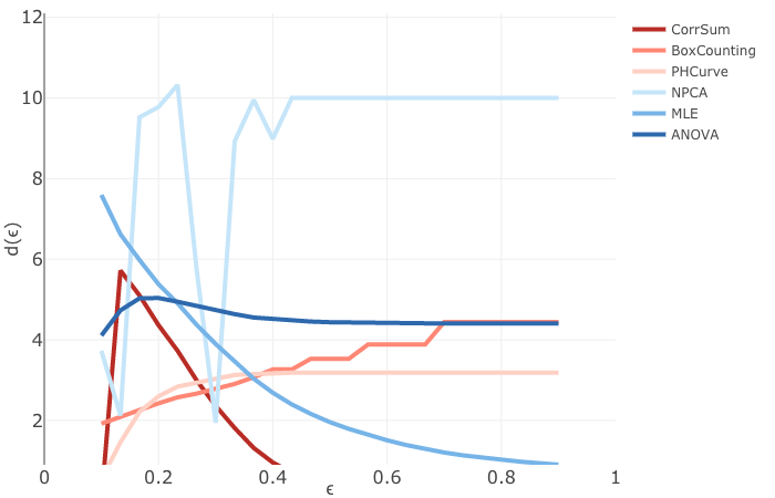
Section 3 addresses the problem of estimating the dimension of $V$ from the sample $\Omega$. We study nonlinear PCA, box counting dimension, persistent homology curve dimension, correlation dimension and the methods of Levina-Bickel [41] and Diaz-Quiroz-Velasco [23]. Each of these notions depends on a parameter $\epsilon$ between $0$ and $1$. This determines the scale from local to global at which we consider $\Omega$. Our empirical dimensions are functions of $\epsilon$. We aggregate their graphs in the dimension diagram of $\Omega$, as seen in Figure 2.

Section 4 links algebraic geometry to topological data analysis. To learn homological information about $V$ from $\Omega$, one wishes to know the reach of the variety $V$. This algebraic number is used to assess the quality of a sample [2, 47]. We propose a variant of persistent homology that incorporates information about the tangent spaces of $V$ at points in $\Omega$.

A key feature of our setting is the existence of polynomials that vanish on the model $V$, extracted from polynomials that vanish on the sample $\Omega$. Linear polynomials are found by Principal Component Analysis (PCA). However, many relevant varieties $V$ are defined by quadratic or cubic equations. Section 5 concerns the computation of these polynomials.

Section 6 utilizes the polynomials found in Section 5. These cut out a variety $V^{\prime}$ that contains $V$. We do not know whether $V^{\prime}=V$ holds, but we would like to test this and certify it, using both numerical and symbolic algorithms. The geography of $\Omega$ inside $V^{\prime}$ is studied by computing dimension, degree, irreducible decomposition, real degree, and volume.

Section 7 introduces our software package LearningAlgebraicVarieties. This is written in Julia [7], and implements all algorithms described in this paper. It is available at

$$\hbox{\url{https://github.com/PBrdng/LearningAlgebraicVarieties.git}}.$$

To compute persistent homology, we use Henselman’s package Eirene [31]. For numerical algebraic geometry we use Bertini [6] and HomotopyContinuation.jl [10]. We conclude with a detailed case study for the dataset in [3, §6.3]. Here, $\Omega$ consists of $6040$ points in $\mathbb{R}^{24}$, representing conformations of the molecule cyclo-octane $C_{8}H_{16}$, shown in Figure 10.

Due to space limitations, many important aspects of learning varieties from samples are not addressed in this article. One is the issue of noise. Clearly, already the slightest noise in one of the points in Figure 1 will let no equation of the form $(x-\alpha)^{2}+(y-\beta)^{2}-\gamma$ vanish on $\Omega$. But some will almost vanish, and these are the equations we are looking for. Based on our experiments, the methods we present for answering questions 1-5 can handle data that is approximate to some extent. However, we leave a qualitative stability analysis for future work. We also assume that there are no outliers in our data. Another aspect of learning varieties is optimization. We might be interested in minimizing a polynomial function $f$ over the unknown variety $V$ by only looking at the samples in $\Omega$. This problem was studied by Cifuentes and Parrilo in [16], using the sum of squares (SOS) paradigm [9].

2 Varieties and Data

The mathematics of data science is concerned with finding low-dimensional needles in high-dimensional haystacks. The needle is the model which harbors the actual data, whereas the haystack is some ambient space. The paradigms of models are the $d$-dimensional linear subspaces $V$ of $\mathbb{R}^{n}$, where $d$ is small and $n$ is large. Most of the points in $\mathbb{R}^{n}$ are very far from any sample $\Omega$ one might ever draw from $V$, even in the presence of noise and outliers.

The data scientist seeks to learn the unknown model $V$ from the sample $\Omega$ that is available. If $V$ is suspected to be a linear space, then she uses linear algebra. The first tool that comes to mind is Principal Component Analysis (PCA). Numerical algorithms for linear algebra are well-developed and fast. They are at the heart of scientific computing and its numerous applications. However, many models $V$ occurring in science and engineering are not linear spaces. Attempts to replace $V$ with a linear approximation are likely to fail.

This is the point where new mathematics comes in. Many branches of mathematics can help with the needles of data science. One can think of $V$ as a topological space, a differential manifold, a metric space, a Lie group, a hypergraph, a category, a semi-algebraic set, and lots of other things. All of these structures are useful in representing and analyzing models.

In this article we focus on the constraints that describe $V$ inside the ambient $\mathbb{R}^{n}$ (or $\mathbb{P}_{\mathbb{R}}^{n-1}$). The paradigm says that these are linear equations, revealed numerically by feeding $\Omega$ to PCA. But, if the constraints are not all linear, then we look for equations of higher degree.

2.1 Algebraic Geometry Basics

Our models $V$ are algebraic varieties over the field $\mathbb{R}$ of real numbers. A variety is the set of common zeros of a system of polynomials in $n$ variables. A priori, a variety lives in Euclidean space $\mathbb{R}^{n}$. In many applications two points are identified if they agree up to scaling. In such cases, one replaces $\mathbb{R}^{n}$ with the real projective space $\mathbb{P}^{n-1}_{\mathbb{R}}$, whose points are lines through the origin in $\mathbb{R}^{n}$. The resulting model $V$ is a real projective variety, defined by homogeneous polynomials in $n$ unknowns. In this article, we use the term variety to mean any zero set of polynomials in $\mathbb{R}^{n}$ or $\mathbb{P}^{n-1}_{\mathbb{R}}$. The following three varieties serve as our running examples.

Example 2.1 (Trott Curve).

The Trott curve is the plane curve of degree four defined by

$$12^{2}(x^{4}+y^{4})\,-\,15^{2}(x^{2}+y^{2})\,+\,350x^{2}y^{2}\,+\,81\,\,\,=\,\,\,0.$$ (1)

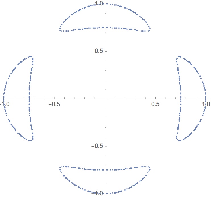
This curve is compact in $\mathbb{R}^{2}$ and has four connected components (see Figure 3). The equation of the corresponding projective curve is obtained by homogenizing the polynomial (1). The curve is nonsingular. The Trott curve is quite special because all of its bitangent lines are all fully real. Plücker showed in 1839 that every plane quartic has $28$ complex bitangents, Zeuthen argued in 1873 that the number of real bitangents is $28$, $16$, $8$ or $4$; see [51, Table 1].

Example 2.2 (Rotation Matrices).

The group ${\rm SO}(3)$ consists of all $3{\times}3$-matrices $X=(x_{ij})$ with ${\rm det}(X)=1$ and $X^{T}X={\rm Id}_{3}$. The last constraint translates into $9$ quadratic equations:

$$\begin{matrix}x_{11}^{2}+x_{21}^{2}+x_{31}^{2}-1&&x_{11}x_{12}+x_{21}x_{22}+x_{31}x_{32}&&x_{11}x_{13}+x_{21}x_{23}+x_{31}x_{33}\\ x_{11}x_{12}+x_{21}x_{22}+x_{31}x_{32}&&x_{12}^{2}+x_{22}^{2}+x_{32}^{2}-1&&x_{12}x_{13}+x_{22}x_{23}+x_{32}x_{33}\\ x_{11}x_{13}+x_{21}x_{23}+x_{31}x_{33}&&x_{12}x_{13}+x_{22}x_{23}+x_{32}x_{33}&&x_{13}^{2}+x_{23}^{2}+x_{33}^{2}-1\end{matrix}$$ (2)

These quadrics say that $X$ is an orthogonal matrix. Adding the cubic ${\rm det}(X)-1$ gives $10$ polynomials that define ${\rm SO}(3)$ as a variety in $\mathbb{R}^{9}$. Their ideal $I$ is prime. In total, there are $20$ linearly independent quadrics in $I$: the nine listed in (2), two from the diagonal of $XX^{T}-{\rm Id}_{3}$, and nine that express the right-hand rule for orientation, like $x_{22}x_{33}-x_{23}x_{32}-x_{11}$.

Example 2.3 (Low Rank Matrices).

Consider the set of $m\times n$-matrices of rank $\leq r$. This is the zero set of $\binom{m}{r+1}\binom{n}{r+1}$ polynomials, namely the $(r+1)$-minors. These equations are homogeneous of degree $r+1$. Hence this variety lives naturally in the projective space $\mathbb{P}^{mn-1}_{\mathbb{R}}$.

A variety $V$ is irreducible if it is not a union of two proper subvarieties. The above varieties are irreducible. A sufficient condition for a variety to be irreducible is that it has a parametrization by rational functions. This holds in Example 2.3 where $V$ consists of the matrices $U_{1}^{T}U_{2}$ where $U_{1}$ and $U_{2}$ have $r$ rows. It also holds for the rotation matrices

$${\footnotesize X\,\,=\,\,\frac{1}{1{-}a^{2}{-}b^{2}{-}c^{2}{-}d^{2}}\begin{pmatrix}1{-}2b^{2}{-}2c^{2}&2ab-2cd&2ac+2bd\\ 2ab+2cd&1{-}2a^{2}{-}2c^{2}&2bc-2ad\\ 2ac-2bd&2bc+2ad&1{-}2a^{2}{-}2b^{2}\end{pmatrix}.}$$ (3)

However, smooth quartic curves in $\mathbb{P}^{2}_{\mathbb{R}}$ admit no such rational parametrization.

The two most basic invariants of a variety $V$ are its dimension and its degree. The former is the length $d$ of the longest proper chain of irreducible varieties $V_{1}\subset V_{2}\subset\cdots\subset V_{d}\subset V$. A general system of $d$ linear equations has a finite number of solutions on $V$. That number is well-defined if we work over $\mathbb{C}$. It is the degree of $V$, denoted ${\rm deg}(V)$. The Trott curve has dimension $1$ and degree $4$. The group ${\rm SO}(3)$ has dimension $3$ and degree $8$. In Example 2.3, if $m=3,n=4$ and $r=2$, then the projective variety has dimension $9$ and degree $6$.

There are several alternative definitions of dimension and degree in algebraic geometry. For instance, they are read off from the Hilbert polynomial, which can be computed by way of Gröbner bases. We refer to Chapter 9, titled Dimension Theory, in the textbook [17].

A variety that admits a rational parametrization is called unirational. Smooth plane curves of degree $\geq 3$ are not unirational. However, the varieties $V$ that arise in applications are often unirational. The reason is that $V$ often models a generative process. This happens in statistics, where $V$ represents some kind of (conditional) independence structure. Examples include graphical models, hidden Markov models and phylogenetic models.

If $V$ is a unirational variety with given rational parametrization, then it is easy to create a finite subset $\Omega$ of $V$. One selects parameter values at random and plugs these into the parametrization. For instance, one creates rank one matrices by simply multiplying a random column vector with a random row vector. A naive approach to sampling from the rotation group ${\rm SO}(3)$ is plugging four random real numbers $a,b,c,d$ into the parametrization (3). Another method for sampling from ${\rm SO}(3)$ will be discussed in Section 7.

Given a dataset $\Omega\subset\mathbb{R}^{n}$ that comes from an applied context, it is reasonable to surmise that the underlying unknown variety $V$ admits a rational parametrization. However, from the vantage point of a pure geometer, such unirational varieties are rare. To sample from a general variety $V$, we start from its defining equations, and we solve ${\rm dim}(V)$ many linear equations on $V$. The algebraic complexity of carrying this out is measured by ${\rm deg}(V)$. See Dufresne et al. [26] for recent work on sampling by way of numerical algebraic geometry.

Example 2.4.

One might sample from the Trott curve $V$ in Example 2.1 by intersecting it with a random line. Algebraically, one solves $\,{\rm dim}(V)=1\,$ linear equation on the curve. That line intersects $V$ in $\,{\rm deg}(V)=4\,$ points. Computing the intersection points can be done numerically, but also symbolically by using Cardano’s formula for the quartic. In either case, the coordinates computed by these methods may be complex numbers. Such points are simply discarded if real samples are desired. This can be a rather wasteful process.

At this point, optimization and real algebraic geometry enter the scene. Suppose that upper and lower bounds are known for the values of a linear function $\ell$ on $V$. In that case, the equations to solve have the form $\ell(x)=\alpha$, where $\alpha$ is chosen between these bounds.

For the Trott curve, we might know that no real points exist unless $|x|\leq 1$. We choose $x$ at random between $-1$ and $+1$, plug it into the equation (1), and then solve the resulting quartic in $y$. The solutions $y$ thus obtained are likely to be real, thus giving us lots of real samples on the curve. Of course, for arbitrary real varieties, it is a hard problem to identify a priori constraints that play the role of $|x|\leq 1$. However, recent advances in polynomial optimization, notably in sum-of-squares programming [9], should be quite helpful.

At this point, let us recap and focus on a concrete instance of the riddles we seek to solve.

Example 2.5.

Let $n=6$, $m=40$ and consider the following forty sample points in $\mathbb{R}^{6}$:

$$\tiny\begin{matrix}(0,-2,6,0,-1,12)&(-4,5,-15,-12,-5,15)\!&(-4,2,-3,2,6,-1)\!&(0,0,-1,-6,0,4)\\ \!\!(12,3,-8,8,-12,2)&\!\!\!\!(20,24,-30,-25,24,-30)\!\!\!&(9,3,5,3,15,1)&\!\!(12,9,-25,20,-15,15)\\ (0,-10,-12,0,8,15)&(15,-6,-4,5,-12,-2)&(3,2,6,6,3,4)&(12,-8,9,9,12,-6)\\ (2,-10,15,-5,-6,25)&(5,-5,0,-3,0,3)&(-12,18,6,-8,9,12)&\!(12,10,-12,-18,8,-15)\\ (1,0,-4,-2,2,0)&(4,-5,0,0,-3,0)&(12,-2,1,6,2,-1)&(-5,0,-2,5,2,0)\\ (3,-2,-8,-6,4,4)&(-3,-1,-9,-9,-3,-3)&(0,1,-2,0,1,-2)&\!\!(5,6,8,10,4,12)\\ (2,0,-1,-1,2,0)&(12,-9,-1,4,-3,-3)&\!\!\!(5,-6,16,-20,-4,24)\!\!&(0,0,1,-3,0,1)\\ \!(15,-10,-12,12,-15,-8)\!\!\!\!&(15,-5,6,6,15,-2)&(-2,1,6,-12,1,6)&(3,2,0,0,-2,0)\\ (24,-20,-6,-18,8,15)&(-3,3,-1,-3,-1,3)&(-10,0,6,-12,5,0)&(2,-2,10,5,4,-5)\\ (4,-6,1,-2,-2,3)&(3,-5,-6,3,-6,-5)&(0,0,-2,3,0,1)&\!(-6,-4,-30,15,12,10)\end{matrix}$$

Where do these samples come from? Do the zero entries or the sign patterns offer any clue?

To reveal the answer we label the coordinates as $(x_{22},x_{21},x_{13},x_{12},x_{23},x_{11})$. The relations

$$\,x_{11}x_{22}-x_{12}x_{21}\,=\,x_{11}x_{23}-x_{13}x_{21}\,=\,x_{12}x_{23}-x_{22}x_{13}\,=\,0$$

hold for all $40$ data points. Hence $V$ is the variety of $2\times 3$-matrices $(x_{ij})$ of rank $\leq 1$. Following Example 2.3, we view this as a projective variety in $\mathbb{P}^{5}_{\mathbb{R}}$. In that ambient projective space, the determinantal variety $V$ is a manifold of dimension $3$ and degree $3$. Note that $V$ is homeomorphic to $\mathbb{P}^{1}_{\mathbb{R}}\times\mathbb{P}^{2}_{\mathbb{R}}$, so we can write its homology groups using the Künneth formula.

In data analysis, proximity between sample points plays a crucial role. There are many ways to measure distances. In this paper we restrict ourselves to two metrics. For data in $\mathbb{R}^{n}$ we use the Euclidean metric, which is induced by the standard inner product ${\langle u,v\rangle=\sum_{i=1}^{n}u_{i}v_{i}}$. For data in $\mathbb{P}^{n-1}_{\mathbb{R}}$ we use the Fubini-Study metric. Points $u$ and $v$ in $\mathbb{P}^{n-1}_{\mathbb{R}}$ are represented by their homogeneous coordinate vectors. The Fubini-Study distance from $u$ to $v$ is the angle between the lines spanned by representative vectors $u$ and $v$ in $\mathbb{R}^{n}$:

$$\mathrm{dist}_{\mathrm{FS}}(u,v)\,\,=\,\,\arccos\frac{|\langle u,v\rangle|}{\|u\|\|v\|}.$$ (4)

This formula defines the unique Riemannian metric on $\mathbb{P}^{n-1}_{\mathbb{R}}$ that is orthogonally invariant.

2.2 A Variety of Varieties

In what follows we present some “model organisms” seen in applied algebraic geometry. Familiarity with a repertoire of interesting varieties is an essential prerequisite for those who are serious about learning algebraic structure from the datasets $\Omega$ they might encounter.

Rank Constraints. Consider $m\times n$-matrices with linear entries having rank $\leq r$. We saw the $r=1$ case in Example 2.3. A rank variety is the set of all tensors of fixed size and rank that satisfy some linear constraints. The constraints often take the simple form that two entries are equal. This includes symmetric matrices, Hankel matrices, Toeplitz matrices, Sylvester matrices, etc. Many classes of structured matrices generalize naturally to tensors.

Example 2.6.

Let $n=\binom{s}{2}$ and identify $\mathbb{R}^{n}$ with the space of skew-symmetric $s\times s$-matrices $P=(p_{ij})$. These satisfy $P^{T}=-P$. Let $V$ be the variety of rank $2$ matrices $P$ in $\mathbb{P}^{n-1}_{\mathbb{R}}$. A parametric representation is given by $p_{ij}=a_{i}b_{j}-a_{j}b_{i}$, so the $p_{ij}$ are the $2\times 2$-minors of a $2\times s$-matrix. The ideal of $V$ is generated by the $4\times 4$ pfaffians $\,p_{ij}p_{kl}-p_{ik}p_{jl}+p_{il}p_{jk}$. These $\binom{s}{4}$ quadrics are also known as the Plücker relations, and $V$ is the Grassmannian of $2$-dimensional linear subspaces in $\mathbb{R}^{s}$. The $r$-secants of $V$ are represented by the variety of skew-symmetric matrices of rank $\leq 2r$. Its equations are the $(2r{+}2)\times(2r{+}2)$ pfaffians of $P$. We refer to [30, Lectures 6 and 9] for an introduction to these classical varieties.

Example 2.7.

The space of $3\times 3\times 3\times 3$ tensors $(x_{ijkl})_{1\leq i,j,k,l\leq 3}$ has dimension $81$. Suppose we sample from its subspace of symmetric tensors $m=(m_{rst})_{0\leq r\leq s\leq t\leq 3}$. This has dimension $n=20$. We use the convention $m_{rst}=x_{ijkl}$ where $r$ is the number of indices $1$ in $(i,j,k,l)$, $s$ is the number of indices $2$, and $t$ is the number of indices $3$. This identifies tensors $m$ with cubic polynomials $m=\sum_{i+j+k\leq 3}m_{ijk}x^{i}y^{j}z^{k}$, and hence with cubic surfaces in $3$-space. Fix $r\in\{1,2,3\}$ and take $V$ to be the variety of tensors $m$ of rank $\leq r$. The equations that define the tensor rank variety $V$ are the $(r+1)\times(r+1)$-minors of the $4\times 10$ Hankel matrix

$${\footnotesize\begin{bmatrix}\,m_{000}\,&\,m_{100}&m_{010}&m_{001}\,&\,m_{200}&m_{110}&m_{101}&m_{020}&m_{011}&m_{002}\,\\ \,m_{100}\,&\,m_{200}&m_{110}&m_{101}\,&\,m_{300}&m_{210}&m_{201}&m_{120}&m_{111}&m_{102}\,\\ \,m_{010}\,&\,m_{110}&m_{020}&m_{011}\,&\,m_{210}&m_{120}&m_{111}&m_{030}&m_{021}&m_{012}\,\\ \,m_{001}\,&\,m_{101}&m_{011}&m_{002}\,&\,m_{201}&m_{111}&m_{102}&m_{021}&m_{012}&m_{003}\,\\ \end{bmatrix}.}$$

See Landsberg’s book [38] for an introduction to the geometry of tensors and their rank.

Example 2.8.

In distance geometry, one encodes finite metric spaces with $p$ points in the Schönberg matrix $\,D\,=\,\bigl{(}d_{ip}+d_{jp}-d_{ij}\bigr{)}\,$ where $d_{ij}$ is the squared distance between points $i$ and $j$. The symmetric $(p{-}1)\times(p{-}1)$ matrix $D$ is positive semidefinite if and only if the metric space is Euclidean, and its embedding dimension is the rank $r$ of $D$. See [21, §6.2.1] for a textbook introduction and derivation of Schönberg’s esults. Hence the rank varieties of the Schönberg matrix $D$ encode the finite Euclidean metric spaces with $p$ points. A prominent dataset corresponding to the case $p=8$ and $r=3$ will be studied in Section 7.

Matrices and tensors with rank constraints are ubiquitous in data science. Make sure to search for such low rank structures when facing vectorized samples, as in Example 2.5.

Hypersurfaces. The most basic varieties are defined by just one polynomial. When given a sample $\Omega$, one might begin by asking for hypersurfaces that contain $\Omega$ and that are especially nice, simple and informative. Here are some examples of special structures worth looking for.

Example 2.9.

For $s=6,r=2$ in Example 2.6, $V$ is the hypersurface of the $6\times 6$-pfaffian:

$${\footnotesize\begin{matrix}\,\,\,\,p_{16}p_{25}p_{34}-p_{15}p_{26}p_{34}-p_{16}p_{24}p_{35}+p_{14}p_{26}p_{35}+p_{15}p_{24}p_{36}\\ -p_{14}p_{25}p_{36}+p_{16}p_{23}p_{45}-p_{13}p_{26}p_{45}+p_{12}p_{36}p_{45}-p_{15}p_{23}p_{46}\\ +p_{13}p_{25}p_{46}-p_{12}p_{35}p_{46}+p_{14}p_{23}p_{56}-p_{13}p_{24}p_{56}+p_{12}p_{34}p_{56}.\end{matrix}}$$ (5)

The $15$ monomials correspond to the matchings of the complete graph with six vertices.

Example 2.10.

The hyperdeterminant of format $2\times 2\times 2$ is a polynomial of degree four in $n=8$ unknowns, namely the entries of a $2\times 2\times 2$-tensor $X=(x_{ijk})$. Its expansion equals

$${\footnotesize\begin{matrix}x_{110}^{2}x_{001}^{2}{+}x_{100}^{2}x_{011}^{2}{+}x_{010}^{2}x_{101}^{2}{+}x_{000}^{2}x_{111}^{2}+4x_{000}x_{110}x_{011}x_{101}{+}4x_{010}x_{100}x_{001}x_{111}-2x_{100}x_{110}x_{001}x_{011}\\ -2x_{010}x_{110}x_{001}x_{101}-2x_{010}x_{100}x_{011}x_{101}{-}2x_{000}x_{110}x_{001}x_{111}{-}2x_{000}x_{100}x_{011}x_{111}{-}2x_{000}x_{010}x_{101}x_{111}.\end{matrix}}$$

This hypersurface is rational and it admits several nice parametrizations, useful for sampling points. For instance, up to scaling, we can take the eight principal minors of a symmetric $3\times 3$-matrix, with $x_{000}=1$ as the $0\times 0$-minor, $x_{100},x_{010},x_{001}$ for the $1\times 1$-minors (i.e. diagonal entries), $x_{110},x_{101},x_{011}$ for the $2\times 2$-minors, and $x_{111}$ for the $3\times 3$-determinant.

Example 2.11.

Let $n=10$, with coordinates for $\mathbb{R}^{10}$ given by the off-diagonal entries of a symmetric $5\times 5$-matrix $(x_{ij})$. There is a unique quintic polynomial in these variables that vanishes on symmetric $5\times 5$-matrices of rank $\leq 2$. This polynomial, known as the pentad, plays a historical role in the statistical theory of factor analysis [25, Example 4.2.8]. It equals

$${\footnotesize\begin{matrix}x_{14}x_{15}x_{23}x_{25}x_{34}-x_{13}x_{15}x_{24}x_{25}x_{34}-x_{14}x_{15}x_{23}x_{24}x_{35}+x_{13}x_{14}x_{24}x_{25}x_{35}\\ +x_{12}x_{15}x_{24}x_{34}x_{35}-x_{12}x_{14}x_{25}x_{34}x_{35}+x_{13}x_{15}x_{23}x_{24}x_{45}-x_{13}x_{14}x_{23}x_{25}x_{45}\\ -x_{12}x_{15}x_{23}x_{34}x_{45}+x_{12}x_{13}x_{25}x_{34}x_{45}+x_{12}x_{14}x_{23}x_{35}x_{45}-x_{12}x_{13}x_{24}x_{35}x_{45}.\end{matrix}}$$

We can sample from the pentad using the parametrization $\,x_{ij}=a_{i}b_{j}+c_{i}d_{j}\,$ for $1\leq i<j\leq 5$.

Example 2.12.

The determinant of the $(p{-}1)\times(p{-}1)$ matrix in Example 2.8 equals the squared volume of the simplex spanned by $p$ points in $\mathbb{R}^{p-1}$. If $p=3$ then we get Heron’s formula for the area of a triangle in terms of its side lengths. The hypersurface in $\mathbb{R}^{\binom{p}{2}}$ defined by this polynomial represents configurations of $p$ points in $\mathbb{R}^{p-1}$ that are degenerate.

One problem with interesting hypersurfaces is that they often have a very high degree and it would be impossible to find that equation by our methods in Section 5. For instance, the Lüroth hypersurface [5] in the space of ternary quartics has degree $54$, and the restricted Boltzmann machine [18] on four binary random variables has degree $110$. These hypersurfaces are easy to sample from, but there is little hope to learn their equations from those samples.

Secret Linear Spaces. This refers to varieties that become linear spaces after a simple change of coordinates. Linear spaces $V$ are easy to recognize from samples $\Omega$ using PCA.

Toric varieties become linear spaces after taking logarithms, so they can be learned by taking the coordinatewise logarithm of the sample points. Formally, a toric variety is the image of a monomial map. Equivalently, it is an irreducible variety defined by binomials.

Example 2.13.

Let $n=6,m=40$ and consider the following dataset in $\mathbb{R}^{6}$:

$$\tiny\begin{matrix}(91,130,169,70,91,130)\!\!&(4,2,1,8,4,2)&(6,33,36,11,12,66)&(24,20,44,30,66,55)\\ (8,5,10,40,80,50)&(11,11,22,2,4,4)&(88,24,72,33,99,27)&(14,77,56,11,8,44)\\ (70,60,45,84,63,54)&(143,13,78,11,66,6)&\!\!(182,91,156,98,168,84)\!&(21,98,91,42,39,182)\\ (5,12,3,20,5,12)&(80,24,8,30,10,3)&(3,5,5,15,15,25)&(10,10,11,10,11,11)\\ (121,66,88,66,88,48)&(45,81,63,45,35,63)&(48,52,12,156,36,39)&(45,50,60,45,54,60)\\ (143,52,117,44,99,36)&(56,63,7,72,8,9)&(10,55,20,11,4,22)&(91,56,7,104,13,8)\\ (24,6,42,4,28,7)&(18,10,18,45,81,45)&(36,27,117,12,52,39)&(3,2,2,3,3,2)\\ (40,10,35,8,28,7)&\!\!(22,10,26,55,143,65)&(132,36,60,33,55,15)&\!\!(98,154,154,77,77,121)\\ (55,20,55,44,121,44)&(24,30,39,40,52,65)&\!(22,22,28,121,154,154)&(6,3,6,4,8,4)\\ (77,99,44,63,28,36)&(30,20,90,6,27,18)&(1,5,2,5,2,10)&(26,8,28,26,91,28)\\ \end{matrix}$$

Replace each of these forty vectors by its coordinate-wise logarithm. Applying PCA to the resulting vectors, we learn that our sample comes from a $4$-dimensional subspace of $\mathbb{R}^{6}$. This is the row space of a $4\times 6$-matrix whose columns are the vertices of a regular octahedron:

$${\footnotesize A\quad=\quad\begin{pmatrix}1&1&1&0&0&0\\ 1&0&0&1&1&0\\ 0&1&0&1&0&1\\ 0&0&1&0&1&1\\ \end{pmatrix}.}$$

Our original samples came from the toric variety $X_{A}$ associated with this matrix. This means each sample has the form $(ab,ac,ad,bc,bd,cd)$, where $a,b,c,d$ are positive real numbers.

Toric varieties are important in applications. For instance, in statistics they correspond to exponential families for discrete random variables. Overlap with rank varieties arises for matrices and tensors of rank $1$. Those smallest rank varieties are known in geometry as the Segre varieties (for arbitrary tensors) and the Veronese varieties (for symmetric tensors). These special varieties are toric, so they are represented by an integer matrix $A$ as above.

Example 2.14.

Let $n=6$ and take $\Omega$ to be a sample of points of the form

$$\bigl{(}\,(2a+b)^{-1},(a+2b)^{-1},(2a+c)^{-1},(a+2c)^{-1},(2b+c)^{-1},(b+2c)^{-1}\,\bigr{)}.$$

The corresponding variety $V\subset\mathbb{P}^{5}_{\mathbb{R}}$ is a reciprocal linear space $V$; see [37]. In projective geometry, such a variety arises as the image of a linear space under the classical Cremona transformation. From the sample we can learn the variety $V$ by replacing each data point by its coordinate-wise inverse. Applying PCA to these reciprocalized data, we learn that $V$ is a surface in $\mathbb{P}_{\mathbb{R}}^{5}$, cut out by ten cubics like $\,2x_{3}x_{4}x_{5}-x_{3}x_{4}x_{6}-2x_{3}x_{5}x_{6}+x_{4}x_{5}x_{6}$.

Algebraic Statistics and Computer Vision. Model selection is a standard task in statistics. The models considered in algebraic statistics [25] are typically semi-algebraic sets, and it is customary to identify them with their Zariski closures, which are algebraic varieties.

Example 2.15.

Bayesian networks are also known as directed graphical models. The corresponding varieties are parametrized by monomial maps from products of simplices. Here are the equations for a Bayesian network on $4$ binary random variables [25, Example 3.3.11]:

$${\footnotesize\begin{matrix}(x_{0000}+x_{0001})(x_{0110}+x_{0111})-(x_{0010}+x_{0011})(x_{0100}+x_{0101}),\\ (x_{1000}+x_{1001})(x_{1110}+x_{1111})-(x_{1010}+x_{1011})(x_{1100}+x_{1101}),\\ x_{0000}x_{1001}-x_{0001}x_{1000},\,x_{0010}x_{1011}-x_{0011}x_{1010},\,x_{0100}x_{1101}-x_{0101}x_{1100},\,x_{0110}x_{1111}-x_{0111}x_{1110}.\end{matrix}}$$

The coordinates $x_{ijkl}$ represent the probabilities of observing the $16$ states under this model.

Computational biology is an excellent source of statistical models with interesting geometric and combinatorial properties. These include hidden variable tree models for phylogenetics, and hidden Markov models for gene annotation and sequence alignment.

In the social sciences and economics, statistical models for permutations are widely used:

Example 2.16.

Let $n=6$ and consider the Plackett-Luce model for rankings of three items [53]. Each item has a model parameter $\theta_{i}$, and we write $x_{ijk}$ for the probability of observing the permutation $ijk$. The model is the surface in $\mathbb{P}^{5}_{\mathbb{R}}$ given by the parametrization

$${\footnotesize\begin{matrix}x_{123}\,=\,\theta_{2}\theta_{3}(\theta_{1}{+}\theta_{3})(\theta_{2}{+}\theta_{3}),&x_{132}\,=\,\theta_{2}\theta_{3}(\theta_{1}{+}\theta_{2})(\theta_{2}{+}\theta_{3}),&x_{213}\,=\,\theta_{1}\theta_{3}(\theta_{1}{+}\theta_{3})(\theta_{2}{+}\theta_{3}),\\ x_{231}\,=\,\theta_{1}\theta_{3}(\theta_{1}{+}\theta_{2})(\theta_{1}{+}\theta_{3}),&x_{312}\,=\,\theta_{1}\theta_{2}(\theta_{1}{+}\theta_{2})(\theta_{2}{+}\theta_{3}),&x_{321}\,=\,\theta_{1}\theta_{2}(\theta_{1}{+}\theta_{2})(\theta_{1}{+}\theta_{3}).\end{matrix}}$$

The prime ideal of this model is generated by three quadrics and one cubic:

$${\footnotesize\begin{matrix}x_{123}(x_{321}+x_{231})-x_{213}(x_{132}+x_{312})\,,\,\,x_{312}(x_{123}+x_{213})-x_{132}(x_{231}+x_{321}),\\ x_{231}(x_{132}+x_{312})-x_{321}(x_{123}+x_{213}),\quad\,x_{123}x_{231}x_{312}-x_{132}x_{321}x_{213}.\end{matrix}}$$

When dealing with continuous distributions, we can represent certain statistical models as varieties in moment coordinates. This applies to Gaussians and their mixtures.

Example 2.17.

Consider the projective variety in $\mathbb{P}_{\mathbb{R}}^{6}$ given parametrically by $m_{0}=1$ and

$${\footnotesize\begin{matrix}m_{1}&=&\lambda\mu+(1-\lambda)\nu\\ m_{2}&=&\lambda(\mu^{2}+\sigma^{2})+(1-\lambda)(\nu^{2}+\tau^{2})\\ m_{3}&=&\lambda(\mu^{3}+3\mu\sigma^{2})+(1-\lambda)(\nu^{3}+3\nu\tau^{2})\\ m_{4}&=&\lambda(\mu^{4}+6\mu^{2}\sigma^{2}+3\sigma^{4})+(1-\lambda)(\nu^{4}+6\nu^{2}\tau^{2}+3\tau^{4})\\ m_{5}&=&\lambda(\mu^{5}+10\mu^{3}\sigma^{2}+15\mu\sigma^{4})+(1-\lambda)(\nu^{5}+10\nu^{3}\tau^{2}+15\nu\tau^{4})\\ m_{6}&=&\lambda(\mu^{6}+15\mu^{4}\sigma^{2}+45\mu^{2}\sigma^{4}+15\sigma^{6})+(1-\lambda)(\nu^{6}+15\nu^{4}\tau^{2}+45\nu^{2}\tau^{4}+15\tau^{6}).\end{matrix}}$$

These are the moments of order $\leq 6$ of the mixture of two Gaussian random variables on the line. Here $\mu$ and $\nu$ are the means, $\sigma$ and $\tau$ are the variances, and $\lambda$ is the mixture parameter. It was shown in [4, Theorem 1] that this is a hypersurface of degree $39$ in $\mathbb{P}^{6}$. For $\mu=0$ we get the Gaussian moment surface which is defined by the $3\times 3$-minors of the $3\times 6$-matrix

$${\footnotesize\begin{pmatrix}0&m_{0}&2m_{1}&3m_{2}&4m_{3}&5m_{4}\\ m_{0}&m_{1}&m_{2}&m_{3}&m_{4}&m_{5}\\ m_{1}&m_{2}&m_{3}&m_{4}&m_{5}&m_{6}\end{pmatrix}.}$$

Example 2.18.

Let $n=9$ and fix the space of $3\times 3$-matrices. An essential matrix is the product of a rotation matrix times a skew-symmetric matrix. In computer vision, these matrices represent the relative position of two calibrated cameras in $3$-space. Their entries $x_{ij}$ serve as invariant coordinates for pairs of such cameras. The variety of essential matrices is defined by ten cubics. These are known as the Démazure cubics [36, Example 2.2].

The article [36] studies camera models in the presence of distortion. For example, the model described in [36, Example 2.3] concerns essential matrices plus one focal length unknown. This is the codimension two variety defined by the $3\times 3$-minors of the $3\times 4$-matrix

$${\footnotesize\begin{pmatrix}\,x_{11}&x_{12}&x_{13}&\,\,x_{21}x_{31}+x_{22}x_{32}+x_{23}x_{33}\\ \,x_{21}&x_{22}&x_{23}&-x_{11}x_{31}-x_{12}x_{32}-x_{13}x_{33}\\ \,x_{31}&x_{32}&x_{33}&0\end{pmatrix}.}$$

Learning such models is important for image reconstruction in computer vision.

3 Estimating the Dimension

The first question one asks about a variety $V$ is “What is the dimension?”. In what follows, we discuss methods for estimating ${\rm dim}(V)$ from the finite sample $\Omega$, taken from $V$. We present six dimension estimates. They are motivated and justified by geometric considerations. For a manifold, dimension is defined in terms of local charts. This is consistent with the notion of dimension in algebraic geometry [17, Chapter 9]. The dimension estimates in this section are based on $\Omega$ alone. Later sections will address the computation of equations that vanish on $V$. These can be employed to find upper bounds on ${\rm dim}(V)$; see (23). In what follows, however, we do not have that information. All we are given is the input $\Omega=\{u^{(1)},\ldots,u^{(m)}\}$.

3.1 Dimension Diagrams

There is an extensive literature (see e.g. [13, 14]) on computing an intrinsic dimension of the sample $\Omega$ from a manifold $V$. The intrinsic dimension of $\Omega$ is a positive real number that approximates the Hausdorff dimension of $V$, a quantity that measures the local dimension of a space using the distances between nearby points. It is a priori not clear that the algebraic definition of ${\rm dim}(V)$ agrees with the topological definition of Hausdorff dimension that is commonly used in manifold learning. However, this will be true under the following natural hypotheses. We assume that $V$ is a variety in $\mathbb{R}^{n}$ or $\mathbb{P}^{n-1}_{\mathbb{R}}$ such that the set of real points is Zariski dense in each irreducible component of $V$. If $V$ is irreducible, then its singular locus ${\rm Sing}(V)$ is a proper subvariety, so it has measure zero. The regular locus $V\backslash{\rm Sing}(V)$ is a real manifold. Each connected component is a real manifold of dimension $\,d={\rm dim}(V)$.

The definitions of intrinsic dimension can be grouped into two categories: local methods and global methods [14, 35]. Definitions involving information about sample neighborhoods fit into the local category, while those that use the whole dataset are called global.

Instead of making such a strict distinction between local and global, we introduce a parameter $0\leq\epsilon\leq 1$. The idea behind this is that $\epsilon$ should determine the range of information that is used to compute the dimension from the local scale ($\epsilon=0$) to the global scale ($\epsilon=1$).

To be precise, for each of the dimension estimates, locality is determined by a notion of distance: the point sample $\Omega$ is a finite metric space. In our context we restrict extrinsic metrics to the sample. For samples $\Omega\subset\mathbb{R}^{n}$ we work with the scaled Euclidean distance

$$\mathrm{dist}_{\mathbb{R}^{n}}(u,v)\,\,\,:=\,\,\,\frac{\|u-v\|}{\max_{x,y\in\Omega}\,\|x-y\|}.$$ (6)

For samples $\Omega$ taken in projective space $\mathbb{P}^{n-1}_{\mathbb{R}}$ we use the scaled Fubini-Study distance

$$\,\,\mathrm{dist}_{\mathbb{P}^{n-1}_{\mathbb{R}}}(u,v)\,\,:=\,\,\frac{\mathrm{dist}_{\mathrm{FS}}(u,v)}{\max_{x,y\in\Omega}\mathrm{dist}_{\mathrm{FS}}(x,y)}.$$ (7)

Two points $u^{(i)}$ and $u^{(j)}$ in $\Omega$ are considered $\epsilon$-close with respect to the parameter $\epsilon$ if $\mathrm{dist}_{\mathbb{R}^{n}}(u,v)\leq\epsilon$ or $\mathrm{dist}_{\mathbb{P}^{n-1}_{\mathbb{R}}}(u,v)\leq\epsilon$, respectively. Given $\epsilon$ we divide the sample $\Omega$ into clusters $\Omega_{1}^{\epsilon},\ldots,\Omega_{l}^{\epsilon}$, which are defined in terms of $\epsilon$-closeness, and apply the methods to each cluster separately, thus obtaining dimension estimates whose definition of being local depends on $\epsilon$. In particular, for $\epsilon=0$ we consider each sample point individually, while for $\epsilon=1$ we consider the whole sample. Intermediate values of $\epsilon$ interpolate between the two.

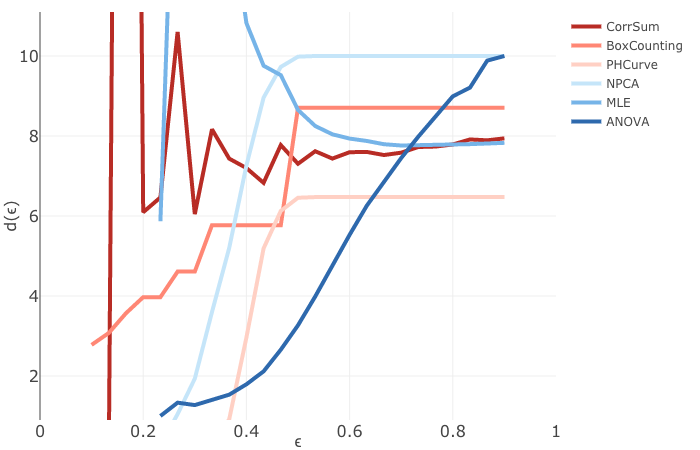
Many of the definitions of intrinsic dimension are consistent. This means that it is possible to compute a scale $\epsilon$ from $\Omega$ for which the intrinsic dimension of each cluster converges to the dimension of $V$ if $m$ is sufficiently large and $\Omega$ is sampled sufficiently densely. By contrast, our paradigm is that $m$ is fixed. For us, $m$ does not tend to infinity. Our standing assumption is that we are given one fixed sample $\Omega$. The goal is to compute a meaningful dimension from that fixed sample of $m$ points. For this reason, we cannot unreservedly employ results on appropriate parameters $\epsilon$ in our methods. The sample $\Omega$ will almost never satisfy the assumptions that are needed. Our approach to circumvent this problem is to create a dimension diagram. Such diagrams are shown in Figures 2, 6, 8 and 11.

Definition 3.1.

Let $\mathrm{dim}(\Omega,\epsilon)$ be one of the subsequent dimension estimates. The dimension diagram of the sample $\Omega$ is the graph of the function $\,(0,1]\to\mathbb{R}_{\geq 0},\,\epsilon\mapsto\mathrm{dim}(\Omega,\epsilon)$.

Remark 3.2.

The idea of using dimension diagrams is inspired by persistent homology. Our dimension diagrams and our persistent homology barcodes of Section 4 both use $\epsilon$ in the interval $[0,1]$ for the horizontal axis. This uniform scale for all samples $\Omega$ makes comparisons across different datasets easier.

The true dimension of a variety is an integer. However, we defined the dimension diagram to be the graph of a function whose range is a subset of the real numbers. The reason is that the subsequent estimates do not return integers. A noninteger dimension can be meaningful mathematically, such as in the case of a fractal curve which fills space densely enough that its dimension could be considered closer to $2$ than $1$. By plotting these diagrams, we hope to gain information about the true dimension $d$ of the variety $V$ from which $\Omega$ was sampled.

Figure 2: Dimension diagrams for 600 points on the variety of $3\times 4$ matrices of rank $2$. This is a projective variety of dimension $9$. Its affine cone has dimension $10$. The left picture shows dimension diagrams for the estimates in Euclidean space $\mathbb{R}^{12}$. The right picture shows those for projective space $\mathbb{P}^{11}_{\mathbb{R}}$. The projective diagrams yield better estimates. The 600 data points were obtained by independently sampling pairs of $4\times 2$ and $2\times 3$ matrices, each with independent entries from the normal distribution, and then multiplying them.

One might be tempted to use the same dimension estimate for $\mathbb{R}^{n}$ and $\mathbb{P}^{n-1}_{\mathbb{R}}$, possibly via the Euclidean distance on an affine patch of $\mathbb{P}_{\mathbb{R}}^{n-1}$. However, the Theorema Egregium by Gauss implies that any projection from $\mathbb{P}_{\mathbb{R}}^{n-1}$ to $\mathbb{R}^{n-1}$ must distort lengths. Hence, because we gave the parameter $\epsilon$ a metric meaning, we must be careful and treat real Euclidean space and real projective space separately.

Each of the curves seen in Figure 2 is a dimension diagram. We used six different methods for estimating the dimension on a fixed sample of $600$ points. For the horizontal axis on the left we took the distance (6) in $\mathbb{R}^{12}$. For the diagram on the right we took (7) in $\mathbb{P}^{11}_{\mathbb{R}}$.

3.2 Six dimension estimates

In this section, we introduce six dimension estimates. They are adapted from the existing literature. Figures 2, 6, 8 and 11 show dimension diagrams generated by our implementation. Judging from those figures, the estimators CorrSum, PHCurve, MLE and ANOVA all perform well on each of the examples. By contrast, NPCA and BoxCounting frequently overestimate the dimension. In general, we found it useful to allow for a “majority vote” for the dimension. That is, we choose as dimension estimate the number which is closest to most of the estimators for a significant (i.e. “persistent”) range of $\epsilon$-values in $[0,1]$.

NPCA Dimension. The gold standard of dimension estimation is PCA. Assuming that $V$ is a linear subspace of $\mathbb{R}^{n}$, we perform the following steps for the input $\Omega$. First, we record the mean $\,\overline{u}:=\frac{1}{m}\sum_{i=1}^{m}u^{(i)}$. Let $M$ be the $m\times n$-matrix with rows $u^{(i)}-\overline{u}$. We compute $\sigma_{1}\geq\cdots\geq\sigma_{\min\{m,n\}}$, the singular values of $M$. The PCA dimension is the number of $\sigma_{i}$ above a certain threshold. For instance, this threshold could be the same as in the definition of the numerical rank in (21) below. Following [39, p. 30], another idea is to set the threshold as $\sigma_{k}$, where ${k={\rm argmax}_{1\leq i\leq\min\{m,n\}-1}|\log_{10}(\sigma_{i+1})-\log_{10}(\sigma_{i})|}$. In our experiments we found that this improved the dimension estimates. In some situations it is helpful to further divide each column of $M$ by its standard deviation. This approach is explained in [39, p. 26].

Using PCA on a local scale is known as Nonlinear Principal Component Analysis (NPCA). Here we partition the sample $\Omega$ into $l$ clusters $\Omega_{1}^{\epsilon},\ldots,\Omega_{l}^{\epsilon}\subset\Omega$ depending on $\epsilon$. For each $\Omega_{i}^{\epsilon}$ we apply the usual PCA and obtain the estimate ${\rm dim}_{\rm pca}(\Omega_{i}^{\epsilon})$. The idea behind this is that the manifold $V\backslash{\rm Sing}(V)$ is approximately linear locally. We take the average of these local dimensions, weighted by the size of each cluster. The result is the nonlinear PCA dimension

$${\rm dim}_{\rm npca}(\Omega,\epsilon)\,\,:=\,\,\,\frac{1}{\sum_{i=1}^{l}|\Omega_{i}^{\epsilon}|}\,\,\sum_{i=1}^{l}|\Omega_{i}^{\epsilon}|\cdot{\rm dim}_{\rm pca}(\Omega_{i}^{\epsilon}).$$ (8)

Data scientists have many clustering methods. For our study we use single linkage clustering. This works as follows. The clusters are the connected components in the graph with vertex set $\Omega$ whose edges are the pairs of points having distance at most $\epsilon$. We do this either in Euclidean space with metric (6), or in projective space with metric (7). In the latter case, the points come from the cone over the true variety $V$. To make $\Omega$ less scattered, we sample a random linear function $l$ and scale each data point $u^{(i)}$ such that $l(u^{(i)})=1$. Then we use those affine coordinates for NPCA. We chose this procedure because NPCA detects linear spaces and the proposed scaling maps projective linear spaces to affine-linear spaces.

We next introduce the notions of box counting dimension, persistent homology curve dimension and correlation dimension. All three of these belong to the class of fractal-based methods, since they rest on the idea of using the fractal dimension as a proxy for ${\rm dim}(V)$.

Box Counting Dimension. Here is the geometric idea in $\mathbb{R}^{2}$. Consider a square of side length $1$ which we cover by miniature squares. We could cover it with $4$ squares of side length $\frac{1}{2}$, or $9$ squares of side length $\frac{1}{3}$, etc. What remains constant is the log ratio of the number of pieces over the magnification factor. For the square: $\frac{\log(4)}{\log(2)}=\frac{\log(9)}{\log(3)}=2$. If $\Omega$ only intersects $3$ out of $4$ smaller squares, then we estimate the dimension to be between $1$ and $2$.

In $\mathbb{R}^{n}$ we choose as a box the parallelopiped with lower vertex ${u^{-}={\rm min}(u^{(1)},\ldots,u^{(m)})}$ and upper vertex ${u^{+}={\rm max}(u^{(1)},\ldots,u^{(m)})}$, where “min” and “max” are coordinatewise minimum and maximum. Thus the box is $\{x\in\mathbb{R}^{n}\,:\,u^{-}\leq x\leq u^{+}\}$. For $j=1,\ldots,n$, the interval $[u^{-}_{j},u^{+}_{j}]$ is divided into $R(\epsilon)$ equally sized intervals, whose length depends on $\epsilon$. A $d$-dimensional object is expected to capture $R(\epsilon)^{d}$ boxes. We determine the number $\nu$ of boxes that contain a point in $\Omega$. Then the box counting dimension estimate is

$$\dim_{\rm box}(\Omega,\epsilon)\,\,:=\,\,\frac{{\rm log}(\nu)}{{\rm log}(R(\epsilon))}.$$ (9)

How to define the function $R(\epsilon)$? Since the number of small boxes is very large, we cannot iterate through all boxes. It is desirable to decide from a data point $u\in\Omega$ in which box it lies. To this end, we set $R(\epsilon)=\lfloor\frac{\lambda}{\epsilon}\rfloor+1$, where $\lambda:=\max_{1\leq j\leq n}|u^{+}_{j}-u^{-}_{j}|$. Then, for $u\in\Omega$ and $k=1,\ldots,n$ we compute the largest $q_{k}$ such that $\frac{q_{k}}{R(\epsilon)}|u^{+}_{k}-u^{-}_{k}|\leq|u_{k}-u^{-}_{k}|$. The $n$ numbers $q_{1},\ldots,q_{n}$ completely determine the box that contains the sample $u$.

For the box counting dimension in real projective space, we represent the points in $\Omega$ on an affine patch of $\mathbb{P}^{n-1}_{\mathbb{R}}$. On this patch we do the same construction as above, the only exception being that “equally sized intervals” is measured in terms of scaled Fubini-Study distance (7).

Persistent Homology Curve Dimension. The underlying idea was proposed by the Pattern Analysis Lab at Colorado State University [50]. First we partition $\Omega$ into $l$ clusters $\Omega_{1}^{\epsilon},\ldots,\Omega_{l}^{\epsilon}$ using single linkage clustering with $\epsilon$. On each subsample $\Omega_{i}$ we construct a minimal spanning tree. Suppose that the cluster $\Omega_{i}$ has $m_{i}$ points. Let $l_{i}(j)$ be the length of the $j$-th longest edge in a minimal spanning tree for $\Omega_{i}$. For each $\Omega_{i}$ we compute

$$\dim_{\rm PHcurve}(\Omega_{i},\epsilon)=\left|\frac{\log(m_{i})}{\log(\frac{1}{m_{i}-1}\sum_{j=1}^{m_{i}-1}l_{i}(j))}\right|.$$

The persistent homology curve dimension estimate $\,\dim_{\rm PHCurve}(\Omega,\epsilon)\,$ is the average of the local dimensions, weighted by the size of each cluster:

$$\dim_{\rm PHcurve}(\Omega,\epsilon)\,\,:=\,\,\frac{1}{\sum_{i=1}^{l}|\Omega_{i}^{\epsilon}|}\sum_{i=1}^{m}|\Omega_{i}|\dim_{\rm PHcurve}(\Omega_{i},\epsilon).$$

In the clustering step we take the distance (6) if the variety is affine and (7) if it is projective.

Correlation Dimension. This is motivated as follows. Suppose that $\Omega$ is uniformly distributed in the unit ball. For pairs $u,v\in\Omega$, we have $\mathrm{Prob}\{\mathrm{dist}_{\mathbb{R}^{n}}(u,v)<\epsilon\}=\epsilon^{d}$, where $d=\mathrm{dim}(V)$. We set $C(\epsilon):=(1/\tbinom{m}{2})\cdot\sum_{1\leq i<j\leq m}\mathbf{1}(\mathrm{dist}_{\mathbb{R}^{n}}(u^{(i)},u^{(j)})<\epsilon)$ , where $\mathbf{1}$ is the indicator function. Since we expect the empirical distribution $C(\epsilon)$ to be approximately $\epsilon^{d}$, this suggests using $\,\frac{\log(C(\epsilon))}{{\rm log}(\epsilon)}\,$ as dimension estimate. In [39, §3.2.6] it is mentioned that a more practical estimate is obtained from $C(\epsilon)$ by selecting some small $h>0$ and putting

$$\qquad\quad\dim_{\rm cor}(\Omega,\epsilon)\,\,:=\,\,\left|\frac{\log C(\epsilon)-\log C(\epsilon+h)}{\log(\epsilon)-\log(\epsilon+h)}\right|.$$ (10)

In practice, we compute the dimension estimates for a finite subset of parameters $\epsilon_{1},\ldots,\epsilon_{k}$ and put $h=\min_{i\neq j}|\epsilon_{i}-\epsilon_{j}|$. The ball in $\mathbb{P}^{n-1}_{\mathbb{R}}$ defined by the scaled Fubini-Study distance (7) is a spherical cap of radius $\epsilon$. Its volume relative to a cap of radius 1 is $\int_{0}^{\epsilon}(\sin\alpha)^{d-1}\mathrm{d}\alpha/\int_{0}^{1}(\sin\alpha)^{d-1}\mathrm{d}\alpha$, which we approximate by $\,\bigl{(}\frac{\sin(\epsilon)}{\sin(1)}\bigr{)}^{d}$. Hence, the projective correlation dimension estimate is

$$\dim_{\rm cor}(\Omega,\epsilon)\,\,:=\,\,\left|\frac{\log C(\epsilon)-\log C(\epsilon+h)}{\log(\sin(\epsilon))-\log(\sin(\epsilon+h))}\right|,\qquad\qquad\qquad$$

with the same $h$ as above and where $C(\epsilon)$ is now computed using the Fubini-Study distance.

We next describe two more methods. They differ from the aforementioned in that they derive from estimating the dimension of the variety $V$ locally at a distinguished point $u^{(\star)}$.

MLE Dimension. Levina and Bickel [41] introduced a maximum likelihood estimator for the dimension of an unknown variety $V$. Their estimate is derived for samples in Euclidean space $\mathbb{R}^{n}$. Let $k$ be the number of samples $u^{(j)}$ in $\Omega$ that are within distance $\epsilon$ to $u^{(\star)}$. We write $T_{i}(u^{(\star)})$ for the distance from $u^{(\star)}$ to its $i$-th nearest neighbor in $\Omega$. Note that $T_{k}(u^{(\star)})\leq\epsilon<T_{k+1}(u^{(\star)})$. The Levina-Bickel formula around the point $u^{(\star)}$ is

$$\dim_{\rm MLE}(\Omega,\epsilon,u^{(\star)})\,\,:=\,\,\left(\frac{1}{k}\sum_{i=1}^{k}\log\frac{\epsilon}{T_{i}(u^{(\star)})}\right)^{-1}.$$ (11)

This expression is derived from the hypothesis that $k=k(\epsilon)$ obeys a Poisson process on the $\epsilon$-neighborhood ${\{u\in\Omega:\mathrm{dist}_{\mathbb{R}^{n}}(u,u^{(\star)})\leq\epsilon\}}$, in which $u$ is uniformly distributed. The formula (11) is obtained by solving the likelihood equations for this Poisson process.

In projective space, we model $k(\epsilon)$ as a Poisson process on $\{u\in\Omega:\mathrm{dist}_{\mathbb{P}_{\mathbb{R}}^{n-1}}(u,u^{(\star)})\leq\epsilon\}$. However, instead of assuming that $u$ is uniformly distributed in that neighborhood, we assume that the orthogonal projection of $u$ onto the tangent space $\mathrm{T}_{u^{(\star)}}\mathbb{P}_{\mathbb{R}}^{n-1}$ is uniformly distributed in the associated ball of radius $\sin{\epsilon}$. Then, we derive the formula

$$\dim_{\rm MLE}(\Omega,\epsilon,u^{(\star)})\,\,:=\,\,\left(\frac{1}{k}\sum_{i=1}^{k}\log\frac{\sin(\epsilon)}{\sin(\widehat{T}_{i}(u^{(\star)}))}\right)^{-1},$$

where $\widehat{T}_{i}(u^{(\star)})$ is the distance from $u^{(\star)}$ to its $i$-th nearest neighbor in $\Omega$ measured for (7).

It is not clear how to choose $u^{(\star)}$ from the given $\Omega$. We chose the following method. Fix the sample neighborhood $\,\Omega_{i}^{\epsilon}:=\{u\in\Omega:\mathrm{dist}_{\mathbb{R}^{n}}(u,u^{(i)})\leq\epsilon\}$. For each $i$ we evaluate the formula (11) for $\Omega_{i}^{\epsilon}$ with distinguished point $u^{(i)}$. With this, the MLE dimension estimate is

$$\dim_{\rm MLE}(\Omega,\epsilon)\,\,:=\,\,\frac{1}{\sum_{i=1}^{m}|\Omega_{i}^{\epsilon}|}\sum_{i=1}^{m}|\Omega_{i}^{\epsilon}|\cdot\dim_{\rm MLE}(\Omega_{i}^{\epsilon},\epsilon,u^{(i)}).$$

ANOVA Dimension. Diaz, Quiroz and Velasco [23] derived an analysis of variance estimate for the dimension of $V$. In their approach, the following expressions are important:

$$\beta_{2s-1}\,=\,\frac{\pi^{2}}{4}-2\sum_{j=0}^{s}\frac{1}{(2j+1)^{2}}\quad\text{and}\quad\beta_{2s}\,=\,\frac{\pi^{2}}{12}-2\sum_{j=0}^{s}\frac{1}{(2j)^{2}}\qquad\text{for}\quad s\in\mathbb{N}.$$ (12)

The quantity $\beta_{d}$ is the variance of the random variable $\Theta_{d}$, defined as the angle between two uniformly chosen random points on the $(d-1)$-sphere. We again fix $\epsilon>0$, and we relabel so that $u^{(1)},\ldots,u^{(k)}$ are the points in $\Omega$ with distance at most $\epsilon$ from $u^{(\star)}$. Let $\theta_{ij}\in[0,\pi]$ denote the angle between $u^{(i)}-u^{(\star)}$ and $u^{(j)}-u^{(\star)}$. Then, the sample covariance of the $\theta_{ij}$ is

$$S\,\,=\,\,\frac{1}{\tbinom{k}{2}}\sum_{1\leq i<j\leq k}\left(\theta_{ij}-\frac{\pi}{2}\right)^{2}.$$ (13)

The analysis in [23] shows that, for small $\epsilon$ and $\Omega$ sampled from a $d$-dimensional manifold, the angles $\theta_{ij}$ are approximately $\Theta_{d}$-distributed. Hence, $S$ is expected to be close to $\beta_{\dim V}$. The ANOVA dimension estimate of $\Omega$ is the index $d$ such that $\beta_{d}$ is closest to $S$:

$$\dim_{\rm ANOVA}(\Omega,\epsilon,u^{(\star)})\,\,:=\,\,{\rm argmin}_{d}\,|\beta_{d}-S|.$$ (14)

As for the MLE estimate, we average (14) over all $u\in\Omega$ being the distinguished point.

To transfer the definition to projective space, we revisit the idea behind the ANOVA estimate. For $u$ close to $u^{(\star)}$, the secant through $u$ and $u^{(\star)}$ is approximately parallel to the tangent space of $V$ at $u^{(\star)}$. Hence, the unit vector $(u^{(\star)}-u)/\|u^{(\star)}-u\|$ is close to being in the tangent space $\mathrm{T}_{u^{(\star)}}(V)$. The sphere in $\mathrm{T}_{u^{(\star)}}(V)$ has dimension $\mathrm{dim}\,V-1$ and we know the variances of the random angles $\Theta_{d}$. To mimic this construction in $\mathbb{P}_{\mathbb{R}}^{n-1}$ we use the angles between geodesics meeting at $u^{(\star)}$. In our implementation, we orthogonally project $\Omega$ to the tangent space $\mathrm{T}_{u^{(\star)}}\mathbb{P}_{\mathbb{R}}^{n-1}$ and compute (13) using coordinates on that space.

We have defined all the mathematical ingredients inherent in our dimension diagrams. Figure 2 now makes sense. Our software and its applications will be discussed in Section 7.

4 Persistent Homology

This section connects algebraic geometry and topological data analysis. It concerns the computation and analysis of the persistent homology [15] of our sample $\Omega$. Persistent homology of $\Omega$ contains information about the shape of the unknown variety $V$ from which $\Omega$ originates.

4.1 Barcodes

Let us briefly review the idea. Given $\Omega$, we associate a simplicial complex with each value of a parameter $\epsilon\in[0,1]$. Just like in the case of the dimension diagrams in the previous section, $\epsilon$ determines the scale at which we consider $\Omega$ from local ($\epsilon=0$) to global ($\epsilon=1$). The complex at $\epsilon=0$ consists of only the vertices and at $\epsilon=1$ it is the full simplex on $\Omega$.

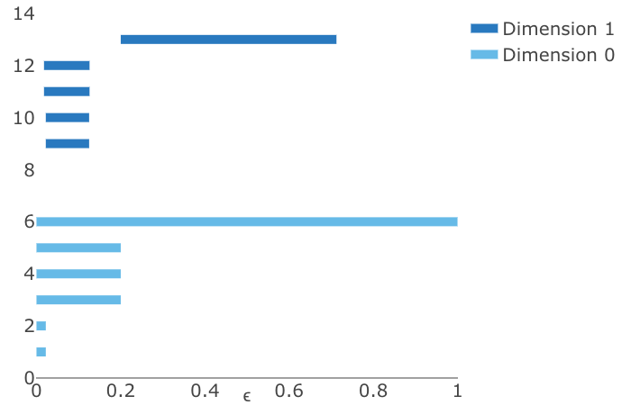
Persistent homology identifies and keeps track of the changes in the homology of those complexes as $\epsilon$ varies. The output is a barcode, i.e. a collection of intervals. Each interval in the barcode corresponds to a topological feature which appears at the value of a parameter given by the left hand endpoint of the interval and disappears at the value given by the right hand endpoint. These barcodes play the same role as a histogram does in summarizing the shape of the data, with long intervals corresponding to strong topological signals and short ones to noise. By plotting the intervals we obtain a barcode, such as the one in Figure 3.

Figure 3: Persistent homology barcodes for the Trott curve.

The most straightforward way to associate a simplicial complex to $\Omega$ at $\epsilon$ is by covering $\Omega$ with open sets $\,U(\epsilon)=\bigcup_{i=1}^{m}U_{i}(\epsilon)$ and then building the associated nerve complex. This is the simplicial complex with vertex set $[m]=\{1,2,\ldots,m\}$, where a subset $\sigma$ of $[m]$ is a face if and only if $\bigcap_{i\in\sigma}U_{i}(\epsilon)\not=\emptyset$. If all nonempty finite intersections of $U_{i}(\epsilon)$ are contractible topological spaces, then the Nerve Lemma guarantees that the homology groups of $U(\epsilon)$ agree with those of its nerve complex. When $U_{i}(\epsilon)$ are $\epsilon$-balls around the data points, i.e.

$$U_{i}(\epsilon)\,:=\,\{v\in\mathbb{R}^{n}:\mathrm{dist}_{\mathbb{R}^{n}}(u^{(i)},v)<\epsilon\}\,\text{ or }\,U_{i}(\epsilon)\,:=\,\{v\in\mathbb{P}_{\mathbb{R}}^{n-1}:\mathrm{dist}_{\mathbb{P}_{\mathbb{R}}^{n-1}}(u^{(i)},v)<\epsilon\},$$ (15)

the nerve complex is called the Čech complex at $\epsilon$. Here $\mathrm{dist}_{\mathbb{R}^{n}}$ and $\mathrm{dist}_{\mathbb{P}_{\mathbb{R}}^{n}}$ are the distances from (6) and (7), respectively. Theorem 4.2 gives a precise statement for a sufficient condition under which the Čech complex of $U(\epsilon)$ built on $\Omega$ yields the correct topology of $V$. However, in practice the hypotheses of the theorem will rarely be satisfied.

Čech complexes are computationally demanding as they require storing simplices in different dimensions. For this reason, applied topologists prefer to work with the Vietoris-Rips complex, which is the flag simplicial complex determined by the edges of the Čech complex. This means that a subset $\sigma\subset[m]$ is a face of the Vietoris-Rips complex if and only if $\,U_{i}(\epsilon)\bigcap U_{j}(\epsilon)\not=\emptyset\,$ for all $i,j\in\sigma$. With the definition in (15), the balls $\,U_{i}(\epsilon)$ and $U_{j}(\epsilon)$ intersect if and only if their centers $u^{(i)}$ and $u^{(j)}$ are less than $2\epsilon$ apart.

Consider the sample from the Trott curve in Figure 3. Following Example 2.4, we sampled by selecting random $x$-coordinates between $-1$ and $1$, and solving for $y$, or vice versa. The picture on the right shows the barcode. This was computed via the Vietoris-Rips complex. For dimensions $0$ and $1$ the six longest bars are displayed. The sixth bar in dimension $1$ is so tiny that we cannot see it. In the range where $\epsilon$ lies between $0$ and $0.2$, we see four components. The barcode for dimension $1$ identifies four persisting features for $\epsilon$ between $0.01$ and $0.12$. Each of these indicates an oval. Once these disappear, another loop appears. This corresponds to the fact that the four ovals are arranged to form a circle. So persistent homology picks up on both intrinsic and extrinsic topological features of the Trott curve.

The repertoire of algebraic geometry offers a fertile testing ground for practitioners of persistent homology. For many classes of algebraic varieties, both over $\mathbb{R}$ and $\mathbb{C}$, one has a priori information about their topology. For instance, the determinantal variety in Example 2.5 is the $3$-manifold $\mathbb{P}_{\mathbb{R}}^{1}\times\mathbb{P}_{\mathbb{R}}^{2}$. Using Henselman’s software Eirene for persistent homology [31], we computed barcodes for several samples $\Omega$ drawn from varieties with known topology.

4.2 Tangent Spaces and Ellipsoids

We underscore the benefits of an algebro-geometric perspective by proposing a variant of persistent homology that performed well in the examples we tested. Suppose that, in addition to knowing $\Omega$ as a finite metric space, we also have information on the tangent spaces of the unknown variety $V$ at the points $u^{(i)}$. This will be the case after we have learned some polynomial equations for $V$ using the methods in Section 5. In such circumstances, we suggest replacing the $\epsilon$-balls in (15) with ellipsoids that are aligned to the tangent spaces.

The motivation is that in a variety with a bottleneck, for example in the shape of a dog bone, the balls around points on the bottleneck may intersect for $\epsilon$ smaller than that which is necessary for the full cycle to appear. When $V$ is a manifold, we design a covering of $\Omega$ that exploits the locally linear structure. Let $0<\lambda<1$. We take $U_{i}(\epsilon)$ to be an ellipsoid around $u^{(i)}$ with principal axes of length $\epsilon$ in the tangent direction of $V$ at $u^{(i)}$ and principal axes of length $\lambda\epsilon$ in the normal direction. In this way, we allow ellipsoids to intersect with their neighbors and thus reveal the true homology of the variety before ellipsoids intersect with other ellipsoids across the medial axis. The parameter $\lambda$ can be chosen by the user. We believe that $\lambda$ should be proportional to the reach of $V$. This metric invariant is defined in the next subsection.

In practice, we perform the following procedure. Let $f=(f_{1},\ldots,f_{k})$ be a vector of polynomials that vanish on $V$, derived from the sample $\Omega\subset\mathbb{R}^{n}$ as in Section 5. An estimator for the tangent space $\mathrm{T}_{u^{(i)}}V$ is the kernel of the Jacobian matrix of $f$ at $u^{(i)}$. In symbols,

$$\widehat{\mathrm{T}}_{u^{(i)}}V\,\,:=\,\,\ker Jf(u^{(i)}).$$ (16)

Let $q_{i}$ denote the quadratic form on $\mathbb{R}^{n}$ that takes value $1$ on $\,\widehat{\mathrm{T}}_{u^{(i)}}V\cap\mathbb{S}^{n-1}\,$ and value $\lambda$ on the orthogonal complement of $\widehat{\mathrm{T}}_{u^{(i)}}V$ in the sphere $\mathbb{S}^{n-1}$. Then, the $q_{i}$ specify the ellipsoids

$$E_{i}\,\,:=\,\,\bigl{\{}\sqrt{q_{i}(x)}\,x\in\mathbb{R}^{n}\,:\,\|x\|\leq 1\bigr{\}}.$$

The role of the $\epsilon$-ball enclosing the $i$th sample point is now played by $U_{i}(\epsilon):=u^{(i)}+\epsilon E_{i}$. These ellipsoids determine the covering $\,U(\epsilon)=\bigcup_{i=1}^{m}U_{i}(\epsilon)\,$ of the given point cloud $\Omega$. From this covering we construct the associated Čech complex or Vietoris-Rips complex.

While using ellipsoids is appealing, it has practical drawbacks. Relating the smallest $\epsilon$ for which $U_{i}(\epsilon)$ and $U_{j}(\epsilon)$ intersect to $\mathrm{dist}_{\mathbb{R}^{n}}(u^{(i)},u^{(j)})$ is not easy. For this reason we implemented the following variant of ellipsoid-driven barcodes. We use the simplicial complex on $[m]$ where

$$\sigma\text{ is a face iff }\,\frac{\mathrm{dist}_{\mathbb{R}^{n}}(u^{(i)},u^{(j)})}{\frac{1}{2}(\sqrt{q_{i}(h)}+\sqrt{q_{j}(h)}\,)}<2\epsilon\,\text{ for all }i,j\in\sigma,\text{ where }h=\frac{u^{(i)}-u^{(j)}}{\|u^{(i)}-u^{(j)}\|}.$$ (17)

In (17) we weigh the distance between $u^{(i)}$ and $u^{(j)}$ by the arithmetic mean of the radii of the two ellipsoids $E_{i}$ and $E_{j}$ in the direction $u^{(i)}-u^{(j)}$. If all quadratic forms $q_{i}$ were equal to $\sum_{j=1}^{n}x_{j}^{2}$, then the simplicial complex of (17) equals the Vietoris-Rips complex from (15).

Figure 4: The left picture shows the barcode constructed from the ellipsoid-driven simplicial complex (17) with $\lambda=0.01$, for the sample from the Trott curve used in Figure 3. For comparison we display the barcode from Figure 3 in the right picture. All relevant topological features persist longer in the left plot.

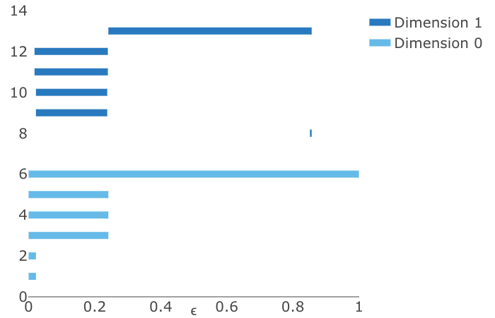
Figure 4 compares the barcodes for the classical Vietoris-Rips complex with those obtained from ellipsoids. It seems promising to further develop variants of persistent homology that take some of the defining polynomial equations for $(\Omega,V)$ into consideration.

4.3 Reaching the Reach

The Čech complex of a covering $U=\bigcup_{i=1}^{m}U_{i}$ has the homology of the union of balls $U$. But, can we give conditions on the sample $\Omega\subset V$ under which a covering reveals the true homology of $V$? A result due to Niyogi, Smale and Weinberger (Theorem 4.2 below) offers an answer in some circumstances. These involve the concept of the reach, which is an important metric invariant of a variety $V$. We here focus on varieties $V$ in the Euclidean space $\mathbb{R}^{n}$.

Definition 4.1.

The medial axis of $V$ is the set $M_{V}$ of all points $u\in\mathbb{R}^{n}$ such that the minimum distance from $V$ to $u$ is attained by two distinct points. The reach $\tau(V)$ is the infimum of all distances from points on the variety $V$ to any point in its medial axis $M_{V}$. In formulas: $\tau(V):=\inf_{u\in V,w\in M_{V}}\|u-w\|$. If $M_{V}=\emptyset$, we define $\tau(V)=+\infty$.

Note that $\tau(V)=+\infty$, if and only if $V$ is an affine-linear subspace. Otherwise, the reach is a non-negative real number. In particular, there exist varieties $V$ with $\tau(V)=0$. For instance, consider the union of two lines $\,V=\{(x,y)\in\mathbb{R}^{2}:xy=0\}$. All points in the diagonal $D=\{(x,y)\in\mathbb{R}^{2}:x=y,x\neq 0\}$ have two closest points on $V$. Hence, $D$ is a subset of the medial axis $M_{V}$, and we conclude that $0\leq\tau(V)\leq\inf_{u\in V,w\in D}\|u-w\|=0$. In general, any singular variety with an “edge” has zero reach.

To illustrate the concept of the reach, let $V$ be a smooth curve in the plane, and draw the normal line at each point of $V$. The collection of these lines is the normal bundle. At a short distance from the curve, the normal bundle is a product: each point $u$ near $V$ has a unique closest point $u^{*}$ on $V$, and $u$ lies on the normal line through $u^{*}$. At a certain distance, however, some of the normal lines cross. If $u$ is a crossing point of minimal distance to $V$, then $u$ has no unique closest point $u^{*}$ on $V$. Instead, there are at least two points on $V$ that are closest to $u$ and the distance from $u$ to each of them is the reach $\tau(V)$. Aamari et al. [2] picture this by writing that “one can roll freely a ball of radius $\tau(V)$ around $V$”.

Niyogi, Smale and Weinberger refer to $\tau(V)^{-1}$ as the “condition number of $V$”. Bürgisser et al. [12] relate $\tau(V)^{-1}$ to the condition number of a semialgebraic set. For the purposes of our survey it suffices to understand how the reach effects the quality of the covering $U(\epsilon)$. The following result is a simplified version of [47, Theorem 3.1], suitable for low dimensions. Note that Theorem 4.2 only covers those varieties $V\subset\mathbb{R}^{n}$ that are smooth and compact.

Theorem 4.2 (Niyogi, Smale, Weinberger 2006).

Let $V\subset\mathbb{R}^{n}$ be a compact manifold of dimension $d\leq 17$, with reach $\tau=\tau(V)$ and $d$-dimensional Euclidean volume $\nu={\rm vol}(V)$. Let $\Omega=\{u^{(1)},\ldots,u^{(m)}\}$ be i.i.d. samples drawn from the uniform probability measure on $V$. Fix $\epsilon=\frac{\tau}{4}$ and $\,\beta=16^{d}\tau^{-d}\nu\,$. For any desired $\delta>0$, fix the sample size at

$$m\,\,>\,\,\,\beta\cdot\bigl{(}\log(\beta)+d+\log(\frac{1}{\delta})\bigr{)}.$$ (18)

With probability $\geq 1-\delta$, the homology groups of the following set coincide with those of $V$:

$$U(\epsilon)\,\,=\,\,\bigcup_{i=1}^{m}\,\bigl{\{}x\in\mathbb{R}^{n}:\|x-u^{(i)}\|<\epsilon\bigr{\}}.$$

A few remarks are in order. First of all, the theorem is stated using the Euclidean distance and not the scaled Euclidean distance (6). However, scaling the distance by a factor $t$ means scaling the volume by $t^{d}$, so the definition of $\beta$ in the theorem is invariant under scaling. Moreover, the theorem has been rephrased in a manner that makes it easier to evaluate the right hand side of (18) in cases of interest. The assumption $d\leq 17$ is not important: it ensures that the volume of the unit ball in $\mathbb{R}^{d}$ can be bounded below by $1$. Furthermore, in [47, Theorem 3.1], the tolerance $\epsilon$ can be any real number between $0$ and $\tau/2$, but then $\beta$ depends in a complicated manner on $\epsilon$. For simplicity, we took $\epsilon=\tau/4$.

Theorem 4.2 gives the asymptotics of a sample size $m$ that suffices to reveal all topological features of $V$. For concrete parameter values it is less useful, though. For example, suppose that $V$ has dimension $4$, reach $\tau=1$, and volume $\nu=1000$. If we desire a 90% guarantee that $U(\epsilon)$ has the same homology as $V$, so $\delta=1/10$, then $m$ must exceed $1,592,570,365$. In addition to that, the theorem assumes that the sample was drawn from the uniform distribution on $V$. But in practice one will rarely meet data that obeys such a distribution. In fact, drawing from the uniform distribution on a curved object is a non-trivial affair [22].

In spite of its theoretical nature, the Niyogi-Smale-Weinberger formula is useful in that it highlights the importance of the reach $\tau(V)$ for analyzing point samples. Indeed, the dominant quantity in (18) is $\beta$, and this grows to the power of $d$ in $\tau(V)^{-1}$. It is therefore of interest to better understand $\tau(V)$ and to develop tools for estimating it.

We found the following formula by Federer [28, Theorem 4.18] to be useful. It expresses the reach of a manifold $V$ in terms of points and their tangent spaces:

$$\qquad\tau(V)\,\,=\inf_{v\neq u\in V}\frac{||u-v||^{2}}{2\delta},\quad\text{ where }\,\,\delta\,=\min_{x\in\mathrm{T}_{v}V}\|(u-v)-x\|.$$ (19)

This formula relies upon knowing the tangent spaces at each point of $u\in V$.

Suppose we are given the finite sample $\Omega$ from $V$. If some equations for $V$ are also known, then we can use the estimator $\widehat{\mathrm{T}}_{u^{(i)}}V$ for the tangent space that was derived in (16). From this we get the following formula for the empirical reach of our sample:

$$\qquad\hat{\tau}(V)\,\,=\,\min_{u,v\in\Omega\atop u\not=v}\frac{||u-v||^{2}}{2\widehat{\delta}},\quad\text{ where }\,\,\widehat{\delta}\,=\min_{x\in\widehat{\mathrm{T}}_{v}V}\|(u-v)-x\|.$$

A similar approach for estimating the reach was proposed by Aamari et al. [2, eqn. (6.1)].

4.4 Algebraicity of Persistent Homology

It is impossible to compute in the field of real numbers $\mathbb{R}$. Numerical computations employ floating point approximations. These are actually rational numbers. Computing in algebraic geometry has traditionally been centered around exact symbolic methods. In that context, computing with algebraic numbers makes sense as well. In this subsection we argue that, in the setting of this paper, most numerical quantities in persistent homology, like the barcodes and the reach, have an algebraic nature. Here we assume that the variety $V$ is defined over $\mathbb{Q}$.

We discuss the work of Horobeţ and Weinstein in [33] which concerns metric properties of a given variety $V\subset\mathbb{R}^{n}$ that are relevant for its true persistent homology. Here, the true persistent homology of $V$, at parameter value $\epsilon$, refers to the homology of the $\epsilon$-neighborhood of $V$. Intuitively, the true persistent homology of the Trott curve is the limit of barcodes as in Figure 3, where more and more points are taken, eventually filling up the entire curve.

An important player is the offset hypersurface $\mathcal{O}_{\epsilon}(V)$. This is the algebraic boundary of the $\epsilon$-neighborhood of $V$. More precisely, for any positive value of $\epsilon$, the offset hypersurface is the Zariski closure of the set of all points in $\mathbb{R}^{n}$ whose distance to $V$ equals $\epsilon$. If $n=2$ and $V$ is a plane curve, then the offset curve $\mathcal{O}_{\epsilon}(V)$ is drawn by tracing circles along $V$.

Figure 5: Offset curves (blue) and the evolute (light blue) of a conic (black).

Example 4.3.

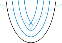
In Figure 5 we examine a conic $V$, shown in black. The light blue curve is its evolute. This is an astroid of degree $6$. The evolute serves as the ED discriminant of $V$, in the context seen in [24, Figure 3]. The blue curves in Figure 5 are the offset curves $\mathcal{O}_{\epsilon}(V)$. These have degree $8$ and are smooth (over $\mathbb{R}$) for small values of $\epsilon$. However, for larger values of $\epsilon$, the offset curves are singular. The transition point occurs at the cusp of the evolute.

It is shown in [33, Theorem 3.4] that the endpoints of bars in the true persistent homology of a variety $V$ occur at numbers that are algebraic over $\mathbb{Q}$. The proof relies on results in real algebraic geometry that characterize the family of fibers in a map of semialgebraic sets.

Example 4.4.

The bars of the barcode in Figure 3 begin and end near the numbers

$$\frac{1}{8}\,=\,0.125\,,\,\quad\frac{\sqrt{24025-217\sqrt{9889}}}{248}\,=\,0.19941426...\,,\,\quad\frac{3}{4}\,=\,0.75.$$

These algebraic numbers delineate the true persistent homology of the Trott curve $V$.

The reach $\tau(V)$ of any real variety $V\subset\mathbb{R}^{n}$ is also an algebraic number. This follows from Federer’s formula (19) which expresses $\tau(V)$ as the optimal value of a polynomial optimization problem. In principle, the reach can be computed in exact arithmetic from the polynomials that define $V$. It remains an open problem how to do this effectively in practice. Eklund’s recent work on bottlenecks [27] represents an important step towards a solution.

At present we do not know a good formula or a tight bound for the algebraic degrees of the barcode and the reach in terms of the invariants of the variety $V$. Deriving such formulas will require a further development and careful analysis of the offset discriminant that was introduced in [33]. We hope to return to this topic in the near future, as it can play a fundamental link between topology and algebraic geometry in the context of data science.

5 Finding Equations

Every polynomial in the ideal $I_{V}$ of the unknown variety $V$ vanishes on the sample $\Omega$. The converse is not true, but it is reasonable to surmise that it holds among polynomials of low degree. The ideal $I_{\Omega}$ of the finite set $\Omega\subset\mathbb{R}^{n}$ can be computed using linear algebra. All our polynomials and ideals in this section lie in the ring $R=\mathbb{R}[x_{1},x_{2},\ldots,x_{n}]$.

5.1 Vandermonde Matrices

Let $\mathcal{M}$ be a finite linearly independent subset of $R$. We write $R_{\mathcal{M}}$ for the $\mathbb{R}$-vector space with basis $\mathcal{M}$ and generally assume that $\mathcal{M}$ is ordered, so that polynomials in $R_{\mathcal{M}}$ can be identified with vectors in $\mathbb{R}^{|\mathcal{M}|}$. Two primary examples for $\mathcal{M}$ are the set of monomials ${\bf x}^{e}=x_{1}^{e_{1}}x_{2}^{e_{2}}\cdots x_{n}^{e_{n}}$ of degree $d$ and the set of monomials of degree at most $d$. We use the notation $R_{d}$ and $R_{\leq d}$ for the corresponding subspaces of $R$. Their dimensions $|\mathcal{M}|$ are

$${\rm dim}(R_{d})\,=\,\binom{n+d-1}{d}\quad{\rm and}\quad{\rm dim}(R_{\leq d})\,=\,\binom{n+d}{d}.$$

We write $U_{\mathcal{M}}(\Omega)$ for the $m\times|\mathcal{M}|$ matrix whose $i$-th row consists of the evaluations of the polynomials in $\mathcal{M}$ at the point $u^{(i)}$. Instead of $U_{\mathcal{M}}(\Omega)$ we write $U_{d}(\Omega)$ when $\mathcal{M}$ contains all monomials of degree $d$ and $U_{\leq d}(\Omega)$ when $\mathcal{M}$ contains monomials of degree $\leq d$.

For example, if $n=1$, $m=3$, and $\Omega=\{u,v,w\}$ then $U_{\leq 3}(\Omega)$ is the Vandermonde matrix

$$U_{\leq 3}(\Omega)=\begin{pmatrix}\,u^{3}&u^{2}&u&1\,\\ \,v^{3}&v^{2}&v&1\,\\ \,w^{3}&w^{2}&w&1\,\end{pmatrix}.$$ (20)

For $n\geq 2$, we call $U_{\mathcal{M}}(\Omega)$ a multivariate Vandermonde matrix. It has the following property:

Remark 5.1.

The kernel of the multivariate Vandermonde matrix $U_{\mathcal{M}}(\Omega)$ equals the vector space $\,I_{\Omega}\cap R_{\mathcal{M}}\,$ of all polynomials that are linear combinations of $\mathcal{M}$ and that vanish on $\Omega$.

The strategy for learning the variety $V$ is as follows. We hope to learn the ideal $I_{V}$ by making an educated guess for the set $\mathcal{M}$. The two desirable properties for $\mathcal{M}$ are:

• The ideal $I_{V}$ of the unknown variety $V$ is generated by its subspace $I_{V}\cap R_{\mathcal{M}}$.

• The inclusion of $I_{V}\cap R_{\mathcal{M}}$ in its superspace $\,I_{\Omega}\cap R_{\mathcal{M}}={\rm ker}(U_{\mathcal{M}}(\Omega))$ is an equality.

There is a fundamental tension between these two desiderata: if $\mathcal{M}$ is too small then (a) will fail, and if $\mathcal{M}$ is too large then (b) will fail. But, of course, suitable sets $\mathcal{M}$ do always exist, since the Hilbert’s Basis Theorem ensures that all ideals in $R$ are finitely generated.

The requirement (b) imposes a lower bound on the size $m$ of the sample. Indeed, $m$ is an upper bound on the rank of $U_{\mathcal{M}}(\Omega)$, since that matrix has $m$ rows. The rank of any matrix is equal to the number of columns minus the dimension of the kernel. This implies:

Lemma 5.2.

If (b) holds, then $\,m\geq|\mathcal{M}|-{\rm dim}(I_{V}\cap R_{\mathcal{M}})$.

In practice, however, the sample $\Omega$ is given and fixed. Thus, we know $m$ and it cannot be increased. The question is how to choose the set $\mathcal{M}$. This leads to some interesting geometric combinatorics. For instance, if we believe that $V$ is homogeneous with respect to some $\mathbb{Z}^{r}$-grading, then it makes sense to choose a set $\mathcal{M}$ that consists of all monomials in a given $\mathbb{Z}^{r}$-degree. Moreover, if we assume that $V$ has a parametrization by sparse polynomials then we would use a specialized combinatorial analysis to predict a set $\mathcal{M}$ that works. A suitable choice of $\mathcal{M}$ can improve the numerical accuracy of the computations dramatically.

In addition to choosing the set of monomials $\mathcal{M}$, we face another problem: how to represent $I_{\Omega}\cap R_{\mathcal{M}}$? Computing a basis for the kernel of $U_{\mathcal{M}}(\Omega)$ yields a set of generators for $I_{\Omega}\cap R_{\mathcal{M}}$. But which basis to use and how to compute it? For instance, the right-singular vectors of $U_{\mathcal{M}}(\Omega)$ with singular value zero yield an orthonormal basis of $I_{\Omega}\cap R_{\mathcal{M}}$. But in applications one often meets ideals $I$ that have sparse generators. This holds in Section 2.

Example 5.3.

Suppose that we obtain a list of $20$ quadrics in nine variables as the result of computing the kernel of a Vandermonde matrix and each quadric looks something like this:

$$-0.037x_{1}^{2}-0.043x_{1}x_{2}-0.011x_{1}x_{3}+0.041x_{1}x_{4}-0.192x_{1}x_{5}+0.034x_{1}x_{6}+0.031x_{1}x_{7}+0.027x_{1}x_{8}+0.271x_{1}x_{9}+0.089x_{2}^{2}-0.009x_{2}x_{3}$$

$$+0.192x_{2}x_{4}+0.041x_{2}x_{5}+0.044x_{2}x_{6}-0.027x_{2}x_{7}+0.031x_{2}x_{8}-0.048x_{2}x_{9}-0.056x_{3}^{2}-0.034x_{3}x_{4}-0.044x_{3}x_{5}+0.041x_{3}x_{6}$$

$$-0.271x_{3}x_{7}+0.048x_{3}x_{8}+0.031x_{3}x_{9}-0.183x_{4}^{2}-0.043x_{4}x_{5}-0.011x_{4}x_{6}+0.039x_{4}x_{7}+0.004x_{4}x_{8}+0.019x_{4}x_{9}-0.057x_{5}^{2}$$

$$-0.009x_{5}x_{6}-0.004x_{5}x_{7}+0.039x_{5}x_{8}-0.35x_{5}x_{9}-0.202x_{6}^{2}-0.019x_{6}x_{7}+0.35x_{6}x_{8}+0.039x_{6}x_{9}-0.188x_{7}^{2}-0.043x_{7}x_{8}-0.011x_{7}x_{9}$$

$$-0.062x_{8}^{2}-0.009x_{8}x_{9}-0.207x_{9}^{2}+0.35x_{1}+0.019x_{2}-0.004x_{3}-0.048x_{4}-0.271x_{5}+0.027x_{6}-0.044x_{7}+0.034x_{8}+0.192x_{9}+0.302$$

This is the first element in an orthonormal basis for $I_{\Omega}\cap R_{\leq 2}$, where $\Omega$ is a sample drawn from a certain variety $V$ in $\mathbb{R}^{9}$. From such a basis, it is very hard to guess what $V$ might be.

It turns out that $V$ is ${\rm SO}(3)$, the group of rotations in $3$-space. After renaming the nine variables, we find the $20$-dimensional space of quadrics mentioned in Example 2.2. However, the quadrics seen in (2) are much nicer. They are sparse and easy to interpret.

For this reason we aim to compute sparse bases of multivariate Vandermonde matrices. There is a trade-off between obtaining sparse basis vectors and stability of the computations. We shall discuss this issue in the next subsection. See Table 1 for a brief summary.

5.2 Numerical Linear Algebra

Computing kernels of matrices of type $U_{\mathcal{M}}(\Omega)$ is a problem in numerical linear algebra. One scenario where the methodology has been developed and proven to work well is the Generalized Principal Component Analysis of Ma et al. [42], where $V$ is a finite union of linear subspaces in $\mathbb{R}^{n}$. For classical Vandermonde matrices, the Bjoerck-Pereyra algorithm [8] accurately computes a LU-decomposition of the Vandermonde matrix; see [32, Section 22]. This decomposition may then be used to compute the kernel. A generalization of this for multivariate Vandermonde matrices of the form $U_{\leq d}(\Omega)$ is given in [48, Theorem 4.4]. To date such a decomposition for $U_{\mathcal{M}}(\Omega)$ is missing for other subsets of monomials $\mathcal{M}$. Furthermore, [48, Theorem 4.4] assumes that the multivariate Vandermonde matrix is square and invertible, but this is never the case in our situation.

In the literature on numerical algebraic geometry, it is standard to represent varieties by point samples, and there are several approaches for learning varieties, and even schemes, from such numerical data. See e.g. [19, 29] and the references therein. From the perspective of commutative algebra, our interpolation problem was studied in e.g. [45, 46].

We developed and implemented three methods based on classical numerical linear algebra:

1. via the R from a QR-decomposition,

2. via a singular value decomposition (SVD), or

3. via the reduced row echelon form (RREF) of $U_{\mathcal{M}}(\Omega)$.

The goal is to compute a (preferably sparse) basis for the kernel of $\,U_{\mathcal{M}}(\Omega)$, with $N=|\mathcal{M}|$. All three methods are implemented in our software. Their descriptions are given below.

QR	slightly less accurate and fast than SVD, yields some sparse basis vectors.
SVD	accurate, fast, but returns orthonormal and hence dense basis.
RREF	no accuracy guarantees, not as fast as the others, gives a sparse basis.

Table 1: The three methods for computing the kernel of the Vandermonde matrix $U_{\mathcal{M}}(\Omega)$.

1 Input: A multivariate Vandermonde matrix $U\in\mathbb{R}^{m\times N}$ and a tolerance value $\tau\geq 0$.

2 Output: A basis for the kernel of $U$.

3 Compute the QR-decomposition $U=QR$, where $Q$ is orthogonal and $R$ is upper triangular;

4 Put $I=\{i:1\leq i\leq N,|R_{ii}|<\tau\}$, $J=[N]\backslash I$, $R^{\prime}=R^{[m]\times J}$ and $\mathcal{B}=\emptyset$;

5 for $i\in I$ do

6      Initialize $a\in\mathbb{R}^{N}$, $a=(a_{1},\ldots,a_{N})$ and put $a_{i}=1$;

7       Solve $R^{\prime}y=R_{i}$ for $y$, where $R_{i}$ is the $i$-th column of $R$.;

8       Put $(a_{1},\ldots,a_{i-1},a_{i+1},\ldots,a_{N})=y$;

9       Update $\mathcal{B}\leftarrow\mathcal{B}\cup\{a\}$;

10      

11 end for

Return $\mathcal{B}$.

Algorithm 1 with_qr

1 Input: A multivariate Vandermonde matrix $U\in\mathbb{R}^{m\times N}$ and a tolerance value $\tau\geq 0$.

2 Output: A basis for the kernel of $U$.

3 Compute the singular value decomposition $U=X\Sigma Y$, where $\Sigma=\mathrm{diag}(\sigma_{1},\ldots,\sigma_{N})$.;

4 Let $k:=\#\{1\leq i\leq N:\sigma_{i}<\tau\}$;

5 Return the last $k$ columns of $Y$;

Algorithm 2 with_svd

1 Input: A multivariate Vandermonde matrix $U\in\mathbb{R}^{m\times N}$ and a tolerance value $\tau\geq 0$.

2 Output: A basis for the kernel of $U$.

3 Compute the reduced row-echelon form $A$ of $U$;

4 Put $I=\{i:1\leq i\leq m,\|A_{i}\|>\sqrt{N}\tau\}$, where $A_{i}$ is the $i$-th row of $A$;

5 Put $B:=A^{I\times[N]}$, $k:=\#I$ and initialize $\mathcal{B}=\emptyset$;

6 For $1\leq i\leq k$ let $j_{i}$ be the position of the first entry in the $i$-th row of $B$ that has absolute value larger than $\tau$ and put $J:=[N]\backslash\{j_{1},\ldots,j_{k}\}$;

7 for $j\in J$ do

8      Put $J^{\prime}:=\{1\leq i\leq N:i<j\}$;

9       Initialize $a\in\mathbb{R}^{N}$, $a=(a_{1},\ldots,a_{N})$ and put $a_{j}=1$ and $a_{i}=0$ for $i\neq j$.;

10       for $i\in J^{\prime}$ do

11             $a_{i}=-B_{i,j}$;

12             Update $\mathcal{B}\leftarrow\mathcal{B}\cup\{a\}$;

13       end for

14      

15 end for

Return $\mathcal{B}$.

Algorithm 3 with_rref

Each of these three methods has its upsides and downsides. These are summarized in Table 1. The algorithms require a tolerance $\tau\geq 0$ as input. This tolerance value determines the numerical rank of the matrix. Let $\sigma_{1}\geq\cdots\geq\sigma_{\min\{m,N\}}$ be the ordered singular values of the $m\times N$ matrix $U$. As in the beginning of Subsection 3.2, the numerical rank of $U$ is

$$r(U,\tau)\,\,:=\,\,\#\bigl{\{}\,i\,\,|\,\,\sigma_{i}\geq\tau\,\bigr{\}}.$$ (21)

Using the criterion in [20, §3.5.1], we can set $\tau=\varepsilon\,\sigma_{1}\,\max\{m,N\}$, where $\epsilon$ is the machine precision. The rationale behind this choice is [20, Corollary 5.1], which says that the round-off error in the $\sigma_{i}$ is bounded by $\|E\|$, where $\|\cdot\|$ is the spectral norm and $U+E$ is the matrix whose singular values were computed. For backward stable algorithms we may use the bound $\|E\|=\mathcal{O}(\varepsilon)\sigma_{1}$. On the other hand, our experiments suggest that an appropriate value for $\tau$ is given by $\frac{1}{2}(\sigma_{i}+\sigma_{i+1})$, for which the jump from $\log_{10}(\sigma_{i})$ to $\log_{10}(\sigma_{i+1})$ is significantly large. This choice is particularly useful for noisy data (as seen in Subsection 7.3). In case of noise the first definition of $\tau$ will likely fail to detect the true rank of $U_{\leq d}(\Omega)$. The reason for this lies in the numerics of Vandermonde matrices, discussed below.

We apply all of the aforementioned to the multivariate Vandermonde matrix $U_{\mathcal{M}}(\Omega)$, for any finite set $\mathcal{M}$ in $R$ that is linearly independent. We thus arrive at the following algorithm.

1 Input: A sample of points $\Omega=\{u^{(1)},u^{(2)},\ldots,u^{(m)}\}\subset\mathbb{R}^{n}$, a finite set $\mathcal{M}$ of monomials in $n$ variables, and a tolerance value $\tau>0$.

2 Output: A basis $\mathcal{B}$ for the kernel of $U_{\mathcal{M}}(\Omega)$;

3 Construct the multivariate Vandermonde matrix $U_{\mathcal{M}}(\Omega)$;

4 Compute a basis $\mathcal{B}$ for the kernel of $U_{\mathcal{M}}(\Omega)$ using Algorithm 1, 2 or 3;

5 Return $\mathcal{B}$;

Algorithm 4 FindEquations

Remark 5.4.

Different sets of quadrics can be obtained by applying Algorithm 4 to a set $\Omega$ of $200$ points sampled uniformly from the group $\mathrm{SO}(3)$. The dense equations in Example 5.3 are obtained using Algorithm 2 (SVD) in Step 4. The more desirable sparse equations from (2) are found when using Algorithm 1 (with QR). In both cases the tolerance was set to be $\tau\approx 4\cdot 10^{-14}\,\sigma_{1}\,$, where $\sigma_{1}$ is the largest singular value of the Vandermonde matrix $U_{\leq 2}(\Omega)$.

Running Algorithm 4 for a few good choices of $\mathcal{M}$ often leads to an initial list of non-zero polynomials that lie in $I_{\Omega}$ and also in $I_{V}$. Those polynomials can then be used to infer an upper bound on the dimension and other information about $V$. This is explained in Section 6. Of course, if we are lucky, we obtain a generating set for $I_{V}$ after a few iterations.

If $m$ is not too large and the coordinates of the points $u^{(i)}$ are rational, then it can be preferable to compute the kernel of $U_{\mathcal{M}}(\Omega)$ symbolically. Gröbner-based interpolation methods, such as the Buchberger-Möller algorithm [45], have the flexibility to select $\mathcal{M}$ dynamically. With this, they directly compute the generators for the ideal $I_{\Omega}$, rather than the user having to worry about the matrices $U_{\leq d}(\Omega)$ for a sequence of degrees $d$. In short, users should keep symbolic methods in the back of their minds when contemplating Algorithm 4.

In the remainder of this section, we discuss numerical issues associated with Algorithm 4. The key step is computing the kernel of the multivariate Vandermonde matrix $U_{\mathcal{M}}(\Omega)$. As illustrated in (20) for samples $\Omega$ on the line $(n=1)$, and $\mathcal{M}$ being all monomials up to a fixed degree, this matrix is a Vandermonde matrix. It is conventional wisdom that Vandermonde matrices are severely ill-conditioned [49]. Consequently, numerical linear algebra solvers are expected to perform poorly when attempting to compute the kernel of $U_{d}(\Omega)$.

One way to circumvent this problem is to use a set of orthogonal polynomials for $\mathcal{M}$. Then, for large sample sizes $m$, two distinct columns of $U_{\mathcal{M}}(\Omega)$ are approximately orthogonal, implying that $U_{\mathcal{M}}(\Omega)$ is well-conditioned. This is because the inner product between the columns associated to $f_{1},f_{2}\in\mathcal{M}$ is approximately the integral of $f_{1}\cdot f_{2}$ over $\mathbb{R}^{n}$. However, a sparse representation in orthogonal polynomials does not yield a sparse representation in the monomial basis. Hence, to get sparse polynomials in the monomials basis from $U_{\mathcal{M}}(\Omega)$, we must employ other methods than the ones presented here. For instance, techniques from compressed sensing may help to compute sparse representations in the monomial basis.

We are optimistic that a numerically-reliable algorithm for computing the kernel of matrices $U_{\leq d}(\Omega)$ exists. The Bjoerck-Pereyra algorithm [8] solves linear equations $Ua=b$ for an $n\times n$ Vandermonde matrix $U$. There is a theoretical guarantee that the computed solution $\hat{a}$ satisfies $|a-\hat{a}|\leq 7n^{5}\epsilon+\mathcal{O}(n^{4}\epsilon^{2})$; see [32, Corollary 22.5]. Hence, $\hat{a}$ is highly accurate – despite $U$ being ill-conditioned. This is confirmed by the experiment mentioned in the beginning of [32, Section 22.3], where a linear system with $\kappa(U)\sim 10^{9}$ is solved with a relative error of $5\epsilon$. We suspect that a Bjoerck-Pereyra-like algorithm together with a thorough structured-perturbation analysis for multivariate Vandermonde matrices would equip us with an accurate algorithm for finding equations. For the present article, we stick with the three methods above, while bearing in mind the difficulties that ill-posedness can cause.

6 Learning from Equations

At this point we assume that the methods in the previous two sections have been applied. This means that we have an estimate $d$ of what the dimension of $V$ might be, and we know a set $\mathcal{P}$ of polynomials that vanish on the finite sample $\Omega\subset\mathbb{R}^{n}$. We assume that the sample size $m$ is large enough so that the polynomials in $\mathcal{P}$ do in fact vanish on $V$. We now use $\mathcal{P}$ as our input. Perhaps the unknown variety $V$ is one of the objects seen in Subsection 2.2.

6.1 Computational Algebraic Geometry

A finite set of polynomials $\mathcal{P}$ in $\mathbb{Q}[x_{1},\ldots,x_{n}]$ is the typical input for algebraic geometry software. Traditionally, symbolic packages like Macaulay2, Singular and CoCoA were used to study $\mathcal{P}$. Buchberger’s Gröbner basis algorithm is the workhorse underlying this approach. More recently, numerical algebraic geometry has emerged, offering lots of promise for innovative and accurate methods in data analysis. We refer to the textbook [6], which centers around the excellent software Bertini. Next to using Bertini, we also employ the Julia package HomotopyContinuation.jl [10]. Both symbolic and numerical methods are valuable for data analysis. The questions we ask in this subsection can be answered with either.

In what follows we assume that the unknown variety $V$ is equal to the zero set of the input polynomials $\mathcal{P}$. We seek to answer the following questions over the complex numbers:

1. What is the dimension of $V$?

2. What is the degree of $V$?

3. Find the irreducible components of $V$ and determine their dimensions and degrees.

Here is an example that illustrates the workflow we imagine for analyzing samples $\Omega$.

Example 6.1.

The variety of Hankel matrices of size $4\times 4$ and rank $2$ has the parametrization

$${\footnotesize\begin{bmatrix}a&b&c&x\\ b&c&x&d\\ c&x&d&e\\ x&d&e&f\end{bmatrix}\quad=\quad\begin{bmatrix}s_{1}^{3}&s_{2}^{3}\\ s_{1}^{2}t_{1}&s_{2}^{2}t_{2}\\ s_{1}t_{1}^{2}&s_{2}t_{2}^{2}\\ t_{1}^{3}&t_{2}^{3}\end{bmatrix}\begin{bmatrix}s_{1}^{3}&s_{1}^{2}t_{1}&s_{1}t_{1}^{2}&t_{1}^{3}\\ s_{2}^{3}&s_{2}^{2}t_{2}&s_{2}t_{2}^{2}&t_{2}^{3}\end{bmatrix}.}$$

Suppose that an adversary constructs a dataset $\Omega$ of size $m=500$ by the following process. He picks random integers $s_{i}$ and $t_{j}$, computes the $4\times 4$-Hankel matrix, and then deletes the antidiagonal coordinate $x$. For the remaining six coordinates he fixes some random ordering, such as $(c,f,b,e,a,d)$. Using this ordering, he lists the $500$ points. This is our input $\Omega\subset\mathbb{R}^{6}$.

We now run Algorithm 4 for the $m\times 210$-matrix $U_{\leq 4}(\Omega)$. The output of this computation is the following pair of quartics which vanishes on the variety $V\subset\mathbb{R}^{6}$ that is described above:

$${\footnotesize\begin{matrix}\mathcal{P}&=&\bigl{\{}\,acf^{2}+ad^{2}f-2ade^{2}-b^{2}f^{2}+2bd^{2}e-c^{2}df+c^{2}e^{2}-cd^{3},\\ &&\quad\,\,\,a^{2}df-a^{2}e^{2}+ac^{2}f-acd^{2}-2b^{2}cf+b^{2}d^{2}+2bc^{2}e-c^{3}d\,\bigr{\}}.\end{matrix}}$$ (22)

Not knowing the true variety, we optimistically believe that the zero set of $\mathcal{P}$ is equal to $V$. This would mean that $V$ is a complete intersection, so it has codimension $2$ and degree $16$.

At this point, we may decide to compute a primary decomposition of $\langle\mathcal{P}\rangle$. We then find that there are two components of codimension $2$, one of degree $3$ and the other of degree $10$. Since $3+10\not=16$, we learn that $\langle\mathcal{P}\rangle$ is not a radical ideal. In fact, the degree $3$ component appears with multiplicity $2$. Being intrigued, we now return to computing equations from $\Omega$.

From the kernel of the $m\times 252$-matrix $U_{5}(\Omega)$, we find two new quintics in $I_{\Omega}$. These only reduce the degree to $3+10=13$. Finally, the kernel of the $m\times 452$-matrix $U_{6}(\Omega)$ suffices. The ideal $I_{V}$ is generated by $2$ quartics, $2$ quintics and $4$ sextics. The mystery variety $V\subset\mathbb{R}^{6}$ has the same dimension and degree as the rank $2$ Hankel variety in $\mathbb{R}^{7}$ whose projection it is.

Our three questions boil down to solving a system $\mathcal{P}$ of polynomial equations. Both symbolic and numerical techniques can be used for that task. Samples $\Omega$ seen in applications are often large, are represented by floating numbers, and have errors and outliers. In those cases, we use Numerical Algebraic Geometry [6, 10]. For instance, in Example 6.1 we intersect (22) with a linear space of dimension $2$. This results in $16$ isolated solutions. Further numerical analysis in step 3 reveals the desired irreducible component of degree $10$.

In the numerical approach to answering the three questions, one proceeds as follows:

1. We add $s$ random (affine-)linear equations to $\mathcal{P}$ and we solve the resulting system in $\mathbb{C}^{n}$. If there are no solutions, then ${\rm dim}(V)<s$. If the solutions are not isolated, then ${\rm dim}(V)>s$. Otherwise, there are finitely many solutions, and ${\rm dim}(V)=s$.

2. The degree of $V$ is the finite number of solutions found in step 1.

3. Using monodromy loops (cf. [6]), we can identify the intersection of a linear space $L$ with any irreducible component of $V_{\mathbb{C}}$ whose codimension equals ${\rm dim}(L)$.

The dimension diagrams from Section 3 can be used to guess a suitable range of values for the parameter $s$ in step 1. However, if we have equations at hand, it is better to determine the dimension $s$ as follows. Let $\mathcal{P}=\{f_{1},\ldots,f_{k}\}$ and $u$ be any data point in $\Omega$. Then, we choose the $s$ from step 1 as the corank of the Jacobian matrix of $f=(f_{1},\ldots,f_{k})$ at $u$; i.e,

$$s:=\mathrm{dim}\,\mathrm{ker}\,Jf(u).$$ (23)

Note that $s=\mathrm{dim}\,V(\mathcal{P})$ as long as $u$ is not a singular point of $V(\mathcal{P})$. In this case, $s$ provides an upper bound for the true dimension of $V$. That is why it is important in step 3 to use higher-dimensional linear spaces $L$ to detect lower-dimensional components of $V(\mathcal{P})$.

Example 6.2.

Take $m=n=3$ in Example 2.3. Let $\mathcal{P}$ consist of the four $2\times 2$-minors that contain the upper-left matrix entry $x_{11}$. The ideal $\langle\mathcal{P}\rangle$ has codimension $3$ and degree $2$. Its top-dimensional components are $\langle x_{11},x_{12},x_{13}\rangle$ and $\langle x_{11},x_{21},x_{31}\rangle$. However, our true model $V$ has codimension $4$ and degree $6$: it is defined by all nine $2\times 2$-minors. Note that $\langle\mathcal{P}\rangle$ is not radical. It also has an embedded prime of codimension $5$, namely $\langle x_{11},x_{12},x_{13},x_{21},x_{31}\rangle$.

6.2 Real Degree and Volume

The discussion in the previous subsection was about the complex points of the variety $V$. The geometric quantity ${\rm deg}(V)$ records a measurement over $\mathbb{C}$. It is insensitive to the geometry of the real points of $V$. That perspective does not distinguish between $\mathcal{P}=\{x^{2}+y^{2}-1\}$ and $\mathcal{P}=\{x^{2}+y^{2}+1\}$. That distinction is seen through the lens of real algebraic geometry.

In this subsection we study metric properties of a real projective variety $V\subset\mathbb{P}^{n}_{\mathbb{R}}$. We explain how to estimate the volume of $V$. Up to a constant depending on $d=\mathrm{dim}\,V$, this volume equals the real degree ${\rm deg}_{\mathbb{R}}(V)$, by which we mean the expected number of real intersection points with a linear subspace of codimension ${\rm dim}(V)$; see Theorem 6.3 below.

To derive these quantities, we use Poincaré’s kinematic formula [34, Theorem 3.8]. For this we need some notation. By [40] there is a unique orthogonally invariant measure $\mu$ on $\mathbb{P}_{\mathbb{R}}^{n}$ up to scaling. We choose the scaling in a way compatible with the unit sphere $\mathbb{S}^{n}$:

$$\mu(\mathbb{P}_{\mathbb{R}}^{n})\,\,=\frac{1}{2}\mathrm{vol}(\mathbb{S}^{n})\,\,=\,\,\frac{\pi^{\frac{n+1}{2}}}{\Gamma(\frac{n+1}{2})}.$$

This makes sense because $\mathbb{P}_{\mathbb{R}}^{n}$ is doubly covered by $\mathbb{S}^{n}$. The $n$-dimensional volume $\mu$ induces a $d$-dimensional measure of volume on $\mathbb{P}^{n}_{\mathbb{R}}$ for any $d=1,2,\ldots,n-1$. We use that measure for $d={\rm dim}(V)$ to define the volume of our real projective variety as $\mathrm{vol}(V):=\mu(V)$.

Let $\mathrm{Gr}(k,\mathbb{P}_{\mathbb{R}}^{n})$ denote the Grassmannian of $k$-dimensional linear spaces in $\mathbb{P}_{\mathbb{R}}^{n}$. This is a real manifold of dimension $(n-k)(k+1)$. Because of the Plücker embedding it is also a projective variety. We saw this for $k=1$ in Example 2.6, but we will not use it here. Again by [40], there is a unique orthogonally invariant measure $\nu$ on $\mathrm{Gr}(k,\mathbb{P}_{\mathbb{R}}^{n})$ up to scaling. We choose the scaling $\nu(\mathrm{Gr}(k,\mathbb{P}_{\mathbb{R}}^{n}))=1$. This defines the uniform probability distribution on the Grassmannian. Poincaré’s Formula [34, Theorem 3.8] states:

Theorem 6.3 (Kinematic formula in projective space).

Let $V$ be a smooth projective variety of codimension $k=n-d$ in $\mathbb{P}^{n}_{\mathbb{R}}$. Then its volume is the volume of $\,\mathbb{P}^{d}_{\mathbb{R}}$ times the real degree:

$$\mathrm{vol}(V)\,=\,\frac{\pi^{\frac{d+1}{2}}}{\Gamma(\frac{d+1}{2})}\cdot{\rm deg}_{\mathbb{R}}(V)\quad\text{where}\quad{\rm deg}_{\mathbb{R}}(V)\,=\,\int_{L\in\mathrm{Gr}(k,\mathbb{P}_{\mathbb{R}}^{n})}\,\#(L\cap V)\,\mathrm{d}\nu.$$

Note that in case of $V$ being a linear space of dimension $d$, we have $\#(L\cap V)=1$ for all $L\in\mathrm{Gr}(n-d,\mathbb{P}_{\mathbb{R}}^{n})$. Hence, $\mathrm{vol}(V)=\mathrm{vol}(\mathbb{P}_{\mathbb{R}}^{d})$, which verifies the theorem in this instance.

The theorem suggests an algorithm. Namely, we sample linear spaces $L_{1},L_{2},\ldots,L_{N}$ independently and uniformly at random, and compute the number $r(i)$ of real points in $V\cap L_{i}$ for each $i$. This can be done symbolically (using Gröbner bases) or numerically (using homotopy continuation). We obtain the following estimator for ${\rm vol}(V)$:

$$\widehat{{\rm vol}}(V)\,\,=\,\,\frac{\pi^{\frac{d+1}{2}}}{\Gamma(\frac{d+1}{2})}\cdot\frac{1}{N}\sum_{i=1}^{N}r(i).$$

We can sample uniformly from $\mathrm{Gr}(k,\mathbb{P}_{\mathbb{R}}^{n})$ by using the following lemma:

Lemma 6.4.

Let $A$ be a random $(k{+}1)\times(n{+}1)$ matrix with independent standard Gaussian entries. The row span of $A$ follows the uniform distribution on the Grassmannian $\mathrm{Gr}(k,\mathbb{P}_{\mathbb{R}}^{n})$.

Proof.

The distribution of the row space of $A$ is orthogonally invariant. Since the orthogonally invariant probability measure on $\mathrm{Gr}(k,\mathbb{P}_{\mathbb{R}}^{n})$ is unique, the two distributions agree. ∎

Example 6.5.

Let $n=2$, $k=1$, and let $V$ be the Trott curve in $\mathbb{P}^{2}_{\mathbb{R}}$. The area of the projective plane $\mathbb{P}^{2}_{\mathbb{R}}$ is half of the surface area of the unit circle: $\mu(\mathbb{P}^{1}_{\mathbb{R}})\,=\,\frac{1}{2}\cdot{\rm vol}(\mathbb{S}^{1})\,=\,\pi$. The real degree of $V$ is computed with the method suggested in Lemma 6.4: ${\rm deg}_{\mathbb{R}}(V)\,=\,1.88364.$ We estimate the length of the Trott curve to be the product of these two numbers: $\,5.91763$. Note that $5.91763$ does not estimate the length of the affine curve depicted in Figure 3, but it is the length of the projective curve defined by the homogenization of the polynomial (1).

Remark 6.6.

Our discussion in this subsection focused on real projective varieties. For affine varieties $V\subset\mathbb{R}^{n}$ there is a formula similar to Theorem 6.3. By [52, (14.70)],

$$\mathrm{vol}(V)\,\,=\,\,\,\frac{O_{n-d}\cdots O_{1}}{O_{n}\cdots O_{d+1}}\cdot\ \int_{L\cap V\neq\emptyset}\#(V\cap L)\,\mathrm{d}L,\qquad d=\mathrm{dim}\,V,$$

where $\mathrm{d}L$ is the density of affine $(n-d)$-planes in $\mathbb{R}^{n}$ from [52, Section 12.2], $\mathrm{vol}(\cdot)$ is Lebesgue measure in $\mathbb{R}^{n}$ and $O_{m}:=\mathrm{vol}\,(\mathbb{S}^{m})$. The problem with using this formula is that in general we do not know how to sample from the density $\mathrm{d}L$ given $L\cap V\neq\emptyset$. The reason is that this distribution depends on $\mathrm{vol}(V)$–which we were trying to compute in the first place.

Suppose that the variety $V$ is the image of a parameter space over which integration is easy. This holds for $V=\mathrm{SO}(3)$, by (3). For such cases, here is an alternative approach for computing the volume: pull back the volume form on $V$ to the parameter space and integrate it there. This can be done either numerically or –if possible– symbolically. Note that this method is not only applicable to smooth varieties, but to any differentiable manifold.

7 Software and Experiments

In this section, we demonstrate how the methods from previous sections work in practice. The implementations are available in our Julia package LearningAlgebraicVarieties. We offer a step-by-step tutorial. To install our software, start a Julia session and type

⬇

Pkg.clone("https://github.com/PBrdng/LearningAlgebraicVarieties.git")

After the installation, the next command is

⬇

using LearningAlgebraicVarieties

This command loads all the functions into the current session. Our package accepts a dataset $\Omega$ as a matrix whose columns are the data points $u^{(1)},u^{(2)},\ldots,u^{(m)}$ in $\mathbb{R}^{n}$.

To use the numerical algebraic geometry software Bertini, we must first download it from https://bertini.nd.edu/download.html. The Julia wrapper for Bertini is installed by

⬇

Pkg.clone("https://github.com/PBrdng/Bertini.jl.git")

The code HomotopyContinuation.jl accepts input from the polynomial algebra package MultivariatePolynomials.jl. The former is described in [10] and it is installed using

⬇

Pkg.add("HomotopyContinuation")

We apply our package to three datasets. The first comes from the group $\mathrm{SO}(3)$, the second from the projective variety $V$ of $2\times 3$-matrices $(x_{ij})$ of rank $1$, and the third from the conformation space of cyclo-octane.

In the first two cases, we draw the samples ourselves. The introduction of [22] mentions algorithms to sample from compact groups. However, for the sake of simplicity we use the following algorithm for sampling from $\mathrm{SO}(3)$. We use Julia’s qr()-command to compute the QR-decomposition of a random real $3\times 3$ matrix with independent standard Gaussian entries and take the $Q$ of that decomposition. If the computation is such that the diagonal entries of $R$ are all positive then, by [44, Theorem 1], the matrix $Q$ is uniformly distributed in $\mathrm{O}(3)$. However, in our case, $Q\in\mathrm{SO}(3)$ and we do not know its distribution.

Our sample from the Segre variety $V=\mathbb{P}^{1}_{\mathbb{R}}\times\mathbb{P}^{2}_{\mathbb{R}}$ in $\mathbb{P}^{5}_{\mathbb{R}}$ is drawn by independently sampling two standard Gaussian matrices of format $2\times 1$ and $1\times 3$ and multiplying them. This procedure yields the uniform distribution on $V$ because the Segre embedding is an isometry under the Fubini-Study metrics on $\mathbb{P}^{1}_{\mathbb{R}},\mathbb{P}^{2}_{\mathbb{R}}$ and $\mathbb{P}^{5}_{\mathbb{R}}$. The third sample, which is $6040$ points from the conformation space of cyclo-octane, is taken from Adams et al. [3, §. 6.3].

We provide the samples used in the subsequent experiments in the JLD data format. After having installed the JLD package in Julia (Pkg.add("JLD")), load the datasets by typing

⬇

import JLD: load

s = string(Pkg.dir("LearningAlgebraicVarieties"),"/datasets.jld")

datasets = load(s)

7.1 Dataset 1: a sample from the rotation group $\mathrm{SO}(3)$

The group $\mathrm{SO}(3)$ is a variety in the space of $3\times 3$-matrices. It is defined by the polynomial equations in Example 2.2. A dataset containing $887$ points from $\mathrm{SO}(3)$ is loaded by typing

⬇

data = datasets["SO(3)"]\end{lstlisting}

Now the current session should contain a variable \lstinline{data} that is a $9\times 887$ matrix.

%Its columns are the data points $u^{(1)},\ldots,u^{(887)}$.

We produce the dimension diagrams by typing

\begin{lstlisting}

DimensionDiagrams(data, false, methods=[:CorrSum,:PHCurve])

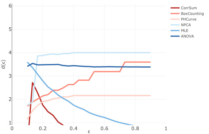
In this command, data is our dataset, the Boolean value is true if we suspect our variety is projective and false otherwise, and methods is any of the dimension estimates :CorrSum, :BoxCounting :PHCurve, :NPCA, :MLE, and :ANOVA. We can leave this unspecified and type

⬇

DimensionDiagrams(data, false)

This command plots all six dimension diagrams. Both outputs are shown in Figure 6.

Figure 6: Dimension diagrams for $887$ points in ${\rm SO}(3)$. The right picture shows all six diagrams described in Subsection 3.2. The left picture shows correlation sum and persistent homology curve dimension estimates.

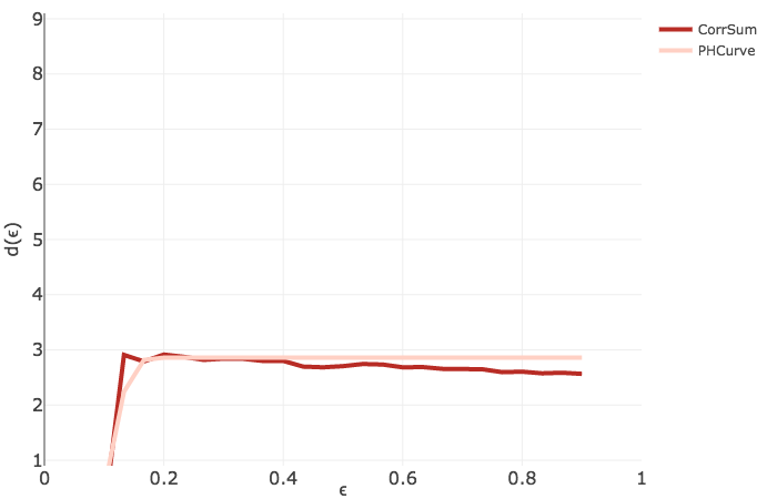
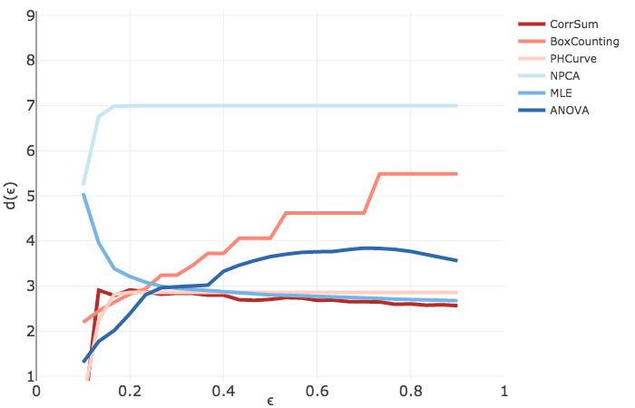
Three estimates are close to $3$, so we correctly guess the true dimension of ${\rm SO}(3)$. In our experiments we found that NPCA and Box Counting Dimension often overestimate.

We proceed by finding polynomials that vanish on the sample. The command we use is

⬇

FindEquations(data, method, d, homogeneous_equations)

where method is one of :with_svd, :with_qr, :with_rref. The degree d refers to the polynomials in $R$ we are looking for. If homogeneous_equations is set to false, then we search in $R_{\leq d}$. If we look for a projective variety then we set it to true, and $R_{d}$ is used. For our sample from ${\rm SO}(3)$ we use the false option. Our sample size $m=887$ is large enough to determine equations up to $d=4$. The following results are found by the various methods:

$d$	method	number of linearly independent equations
$1$	SVD	0
$2$	SVD	20
$2$	QR	20
$2$	RREF	20
$3$	SVD	136
$4$	SVD	550

The correctness of these numbers can be verified by computing (e.g. using Macaulay2) the affine Hilbert function [17, §9.3] of the ideal with the generators in Example 2.2. If we type

⬇

f = FindEquations(data, :with_qr, 2, false)

then we get a list of 20 polynomials that vanish on the sample.

The output is often difficult to interpret, so it can be desirable to round the coefficients:

⬇

round.(f)

The precision can be specified, the default being to the nearest integer. We obtain the output

$$\begin{array}[]{l}x_{1}x_{4}+x_{2}x_{5}+x_{3}x_{6},\\ x_{1}x_{7}+x_{2}x_{8}+x_{3}x_{9}.\end{array}$$

Let us continue analyzing the 20 quadrics saved in the variable f. We use the following command in Bertini to determine whether our variety is reducible and compute its degree:

⬇

import Bertini: bertini

bertini(round.(f), TrackType = 1, bertini_path = p1)

Here p1 is the path to the Bertini binary. Bertini confirms that the variety is irreducible of degree $8$ and dimension $3$ (cf. Figure 6).

Using Eirene we construct the barcodes depicted in Figure 7. We run the following commands to plot barcodes for a random subsample of $250$ points in ${\rm SO}(3)$:

⬇

# sample 250 random points

i = rand(1:887, 250)

# compute the scaled Euclidean distances

dists = ScaledEuclidean(data[:,i])

# pass distance matrix to Eirene and plot barcodes in dimensions up to 3

C = eirene(dists, maxdim = 3)

barcode_plot(C, [0,1,2,3], [8,8,8,8])

The first array [0,1,2,3] of the barcode_plot() function specifies the desired dimensions. The second array [8,8,8,8] selects the 8 largest barcodes for each dimension. If the user does not pass the last array to the function, then all the barcodes are plotted. To compute barcodes arising from the complex specified in (17), we type

⬇

dists = EllipsoidDistances(data[:,i], f, 1e-5)

C = eirene(dists, maxdim = 3)

barcode_plot(C, [0,1,2,3], [8,8,8,8])

Here, f = FindEquations(data, :with_qr, 2, false) is the vector of $20$ quadrics. The third argument of EllipsoidDistances is the parameter $\lambda$ from (17). It is here set to $10^{-5}$.

Figure 7: Barcodes for a subsample of $250$ points from $\mathrm{SO}(3)$. The left picture shows the standard Vietoris-Rips complex, while that on the right comes from the ellipsoid-driven complex (17). Neither reveals any structures in dimension 3, though $V=\mathrm{SO}(3)$ is diffeomorphic to $\mathbb{P}^{3}_{\mathbb{R}}$ and has a non-vanishing $H_{3}(V,\mathbb{Z})$.

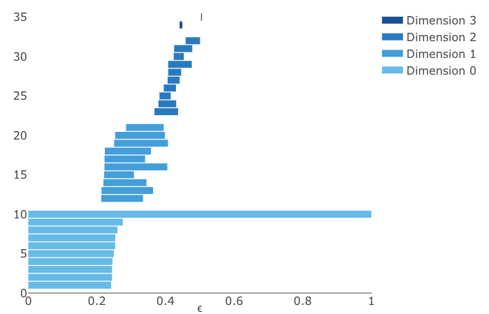
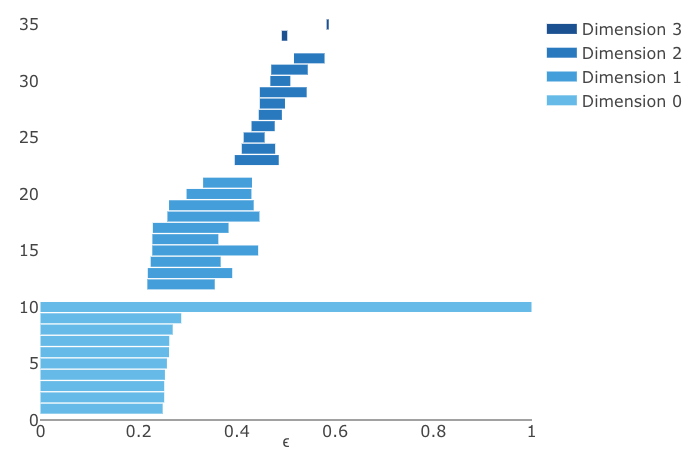
Our subsample of $250$ points is not dense enough to reveal features except in dimension $0$. Instead of randomly selecting the points in the subsample, one could also use the sequential maxmin landmark selector [3, §5.2]. Subsamples chosen this way tend to cover the dataset and to be spread apart from each other. One might also improve the result by constructing different complexes, for example, the lazy witness complexes in [3, §5]. However, this is not implemented in Eirene at present.

7.2 Dataset 2: a sample from the variety of rank one $2\times 3$-matrices

The second sample consists of $200$ data points from the Segre variety $\mathbb{P}^{1}_{\mathbb{R}}\times\mathbb{P}^{2}_{\mathbb{R}}$ in $\mathbb{P}^{5}_{\mathbb{R}}$, that is Example 2.3 with $m=n=3,\,r=1$. We load our sample into the Julia session by typing

⬇

data = datasets["2x3 rank one matrices"]

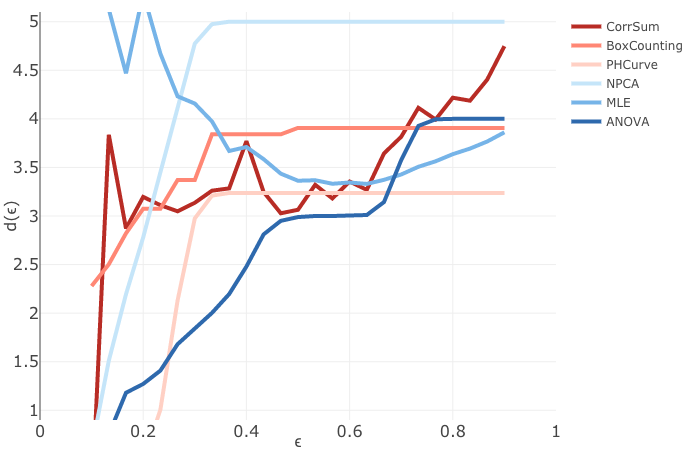
We try the DimensionDiagrams command once with the Boolean value set to false (Euclidean space) and once with the value set to true (projective space). The diagrams are depicted in Figure 8. As the variety $V$ naturally lives in $\mathbb{P}^{5}_{\mathbb{R}}$, the projective diagrams yield better estimates and hint that the dimension is either $3$ or $4$. The true dimension in $\mathbb{P}^{5}_{\mathbb{R}}$ is $3$.

Figure 8: Dimension diagrams for 200 points on the variety of $2\times 3$ matrices of rank $1$. The left picture shows dimension diagrams for the estimates in $\mathbb{R}^{6}$. The right picture shows those for projective space $\mathbb{P}^{5}_{\mathbb{R}}$.

The next step is to find polynomials that vanish. We set homogeneous_equations to true and $d=2$: f = FindEquations(data, method, 2, true). All three methods, SVD, QR and RREF, correctly report the existence of three quadrics. The equations obtained with QR after rounding are as desired:

$$x_{1}x_{4}-x_{2}x_{3}=0,\quad x_{1}x_{6}-x_{2}x_{5}=0,\quad x_{3}x_{6}-x_{4}x_{5}=0.$$

Running Bertini we verify that $V$ is an irreducible variety of dimension $3$ and degree $3$.

We next estimate the volume of $V$ using the formula in Theorem 6.3. We intersect $V$ with $500$ random planes in $\mathbb{P}^{5}_{\mathbb{R}}$ and count the number of real intersection points. We must initialize $500$ linear functions with Gaussian entries involving the same variables as f:

⬇

import MultivariatePolynomials: variables

X = variables(f)

Ls = [randn(3, 6) * X for i in 1:500]

Now, we compute the real intersection points using HomotopyContinuation.jl.

⬇

using HomotopyContinuation

r = map(Ls) do L

# we multiply with a random matrix to make the system square

S = solve([randn(2,3) * f; L])

# check which are solutions to f and return the real ones

vals = [[fi(X => s) for fi in f] for s in solutions(S)]

i = find(norm.(vals) .< 1e-10)

return length(real(S[i]))

end

The command pi^2 * mean(r) reports an estimate of $19.8181$ for the volume of $V$. The true volume of $V$ is the length of $\mathbb{P}^{1}_{\mathbb{R}}$ times the area of $\mathbb{P}^{2}_{\mathbb{R}}$, which is $\pi\cdot(2\pi)=19.7392$.

Figure 9: Barcodes for $200$ points on the Segre variety of $2\times 3$ matrices of rank $1$. The true mod $2$ Betti numbers of $\mathbb{P}^{1}_{\mathbb{R}}\times\mathbb{P}^{2}_{\mathbb{R}}$ are $1,2,2,1$. The left picture shows the barcodes for the usual Vietoris-Rips complex computed using scaled Fubini-Study distance. The right picture is computed using the scaled Euclidean distance. Using the Fubini-Study distance yields better results.

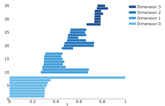
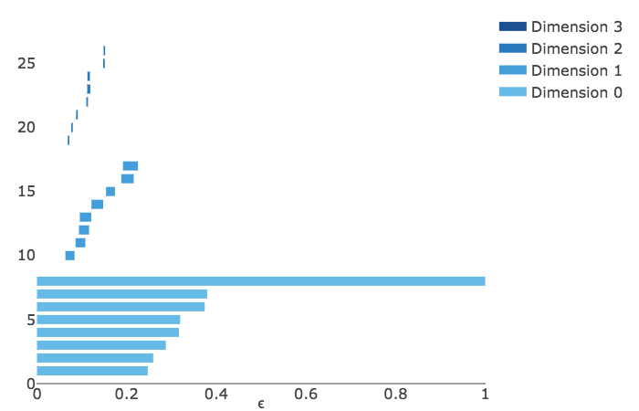
Using Eirene, we construct the barcodes depicted in Figure 9. The barcodes constructed using Fubini-Study distance detect persistent features in dimensions $0$, $1$ and $2$. The barcodes using Euclidean distance only have a strong topological signal in dimension $0$.

7.3 Dataset 3: conformation space of cyclo-octane

Our next variety $V$ is the conformation space of the molecule cyclo-octane $C_{8}H_{16}$. We use the same sample $\Omega$ of $6040$ points that was analyzed in [3, §.6.3]. Cyclo-octane consists of eight carbon atoms arranged in a ring and each bonded to a pair of hydrogen atoms (see Figure 10). The location of the hydrogen atoms is determined by that of the carbon atoms due to energy minimization. Hence, the conformation space of cyclo-octane consists of all possible spatial arrangements, up to rotation and translation, of the ring of carbon atoms.

Figure 10: A cyclo-octane molecule.

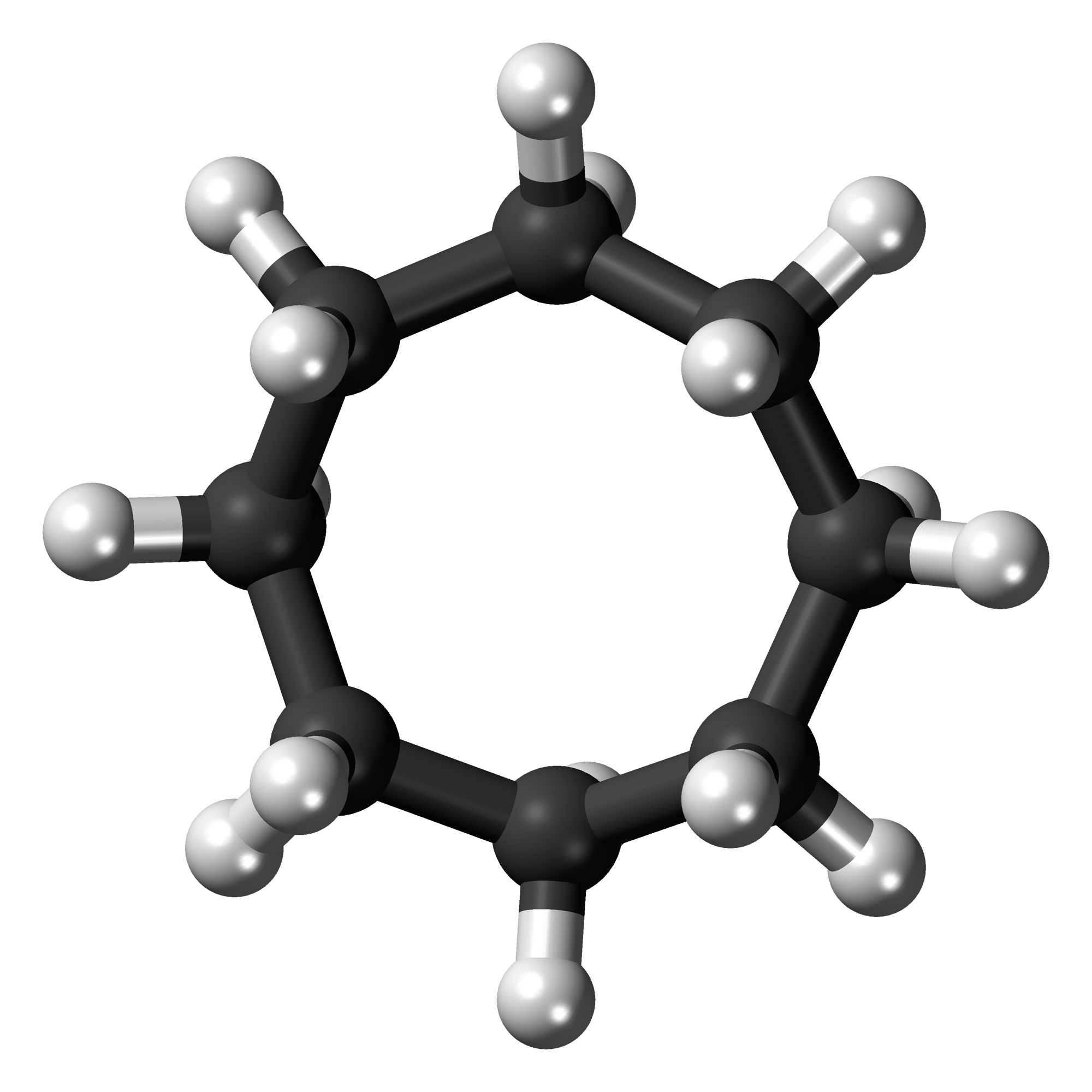
Each conformation is a point in $\mathbb{R}^{24}=\mathbb{R}^{8\cdot 3}$, which represents the coordinates of the carbon atoms $\{z_{0},\dots,z_{7}\}\subset\mathbb{R}^{3}$. Every carbon atom $z_{i}$ forms an isosceles triangle with its two neighbors with angle $\frac{2\pi}{3}$ at $z_{i}$. By the law of cosines, there is a constant $c>0$ such that the squared distances $\,d_{i,j}=\|z_{i}-z_{j}\|^{2}\,$ satisfy

$$d_{i,i+1}\,=\,c\quad\hbox{and}\quad d_{i,i+2}\,=\,\frac{8}{3}c\quad\hbox{for all $i\,\,$ (mod~{}$8$).}$$ (24)

Thus we expect to find $16$ quadrics from the given data. In our sample we have $c\approx 2.21$.

The conformation space is defined modulo translations and rotation; i.e., modulo the $6$-dimensional group of rigid motions in $\mathbb{R}^{3}$. An implicit representation of this quotient space arises by substituting (24) into the Schönberg matrix of Example 2.8 with $p=8$ and $r=3$.

However, the given $\Omega$ lives in $\mathbb{R}^{24}=\mathbb{R}^{8\cdot 3}$, i.e. it uses the coordinates of the carbon atoms. Since the group has dimension $6$, we expect to find $6$ equations that encode a normal form. That normal form is a distinguished representative from each orbit of the group action.

Figure 11: Dimension diagrams for $420$ points from the cyclo-octane dataset.

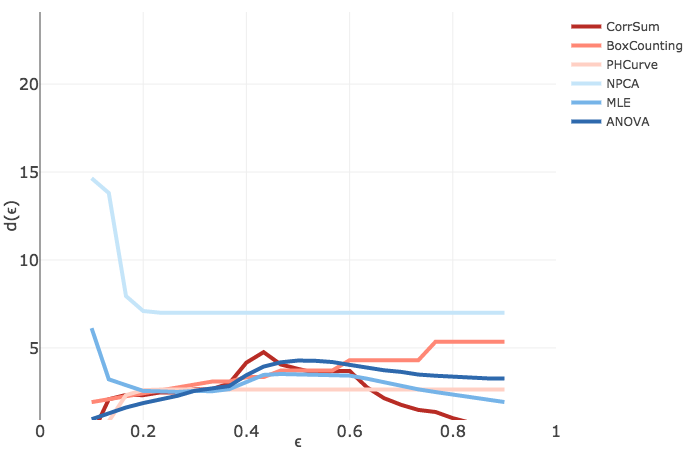
Brown et al. [11] and Martin et al. [43] show that the conformation space of cyclo-octane is the union of a sphere with a Klein bottle, glued together along two circles of singularities. Hence, the dimension of $V$ is $2$, and it has Betti numbers $1,1,2$ in mod $2$ coefficients.

To accelerate the computation of dimension diagrams, we took a random subsample of $420$ points. The output is displayed in Figure 11. A dimension estimate of $2$ seems reasonable:

⬇

i = rand(1:6040, 420)

DimensionDiagrams(data[:,i], false)

The dataset $\Omega$ is noisy: each point is rounded to $4$ digits. Direct use of FindEquations() yields no polynomials vanishing on $\Omega$. The reason is that our code sets the tolerance with the numerical rank in (21). For noisy samples, we must set the tolerance manually. To get a sense for adequate tolerance values, we first compute the multivariate Vandermonde matrix $U_{\leq d}(\Omega)$ and then plot the base 10 logarithms of its singular values. We start with $d=1$.

⬇

import PlotlyJS

M = MultivariateVandermondeMatrix(data, 1, false)

s = log10.(svdvals(M.Vandermonde))

p = PlotlyJS.scatter(; y=s, mode="lines", line_width = 4)

PlotlyJS.Plot(p)

This code produces the left plot in Figure 12. This graph shows a clear drop from $-0.2$ to $-2.5$. Picking the in-between value $-1$, we set the tolerance at $\tau=10^{-1}$. Then, we type

⬇

f = FindEquations(M, method, 1e-1)

where method is one of our three methods. For this tolerance value we find six linear equations. Computed using :with_qr and rounded to three digits, they are as follows:

$$\mathrm{1.}\quad -1.2x_{1}-3.5x_{2}+1.2x_{3}-4.2x_{4}-4.1x_{5}+3.9x_{6}-5.4x_{7}-2.0x_{8}+4.9x_{9}-5.4x_{10}+2.2x_{11}+4.9x_{12}$$

$$\hskip 56.9055pt-4.2x_{13}+4.3x_{14}+3.8x_{15}-1.1x_{16}+3.6x_{17}+x_{18}$$

$$\mathrm{2.}\quad -0.6x_{1}-1.3x_{2}-2.0x_{4}-1.3x_{5}-2.5x_{7}-2.5x_{10}+x_{11}-2.0x_{13}+2.4x_{14}-0.5x_{16}+2.3x_{17}+x_{20}$$

$$\mathrm{3.}\quad 2.5x_{1}+8.1x_{2}-4.0x_{3}+9.2x_{4}+9.6x_{5}-10.5x_{6}+11.4x_{7}+4.7x_{8}-11.5x_{9}+12.6x_{10}-5.1x_{11}$$

$$\hskip 56.9055pt-10.5x_{12}+9.4x_{13}-10.0x_{14}-6.5x_{15}+1.9x_{16}-8.3x_{17}-1.1x_{19}+x_{21}$$

$$\mathrm{4.}\quad x_{1}+x_{4}+x_{7}+x_{10}+x_{13}+x_{16}+x_{19}+x_{22}$$

$$\mathrm{5.}\quad 0.6x_{1}+2.3x_{2}+2.0x_{4}+2.3x_{5}+2.5x_{7}+x_{8}+2.5x_{10}+2.0x_{13}-1.4x_{14}+0.5x_{16}-1.3x_{17}+x_{23}$$

$$\mathrm{6.}\quad -1.3x_{1}-4.6x_{2}+3.8x_{3}-4.9x_{4}-5.5x_{5}+7.5x_{6}-6.0x_{7}-2.7x_{8}+7.5x_{9}-7.2x_{10}+2.9x_{11}+6.5x_{12}$$

$$\hskip 56.9055pt-5.2x_{13}+5.7x_{14}+3.7x_{15}-0.8x_{16}+4.7x_{17}+1.1x_{19}+x_{24}$$

We add the second and the fifth equation, and we add the first, third and sixth, by typing f[2]+f[5] and f[1]+f[3]+f[6] respectively. Together with f[1] we get the following:

$$\begin{matrix}&x_{1}+x_{4}+x_{7}+x_{10}+x_{13}+x_{16}+x_{19}+x_{22}\\ &x_{2}+x_{5}+x_{8}+x_{11}+x_{14}+x_{17}+x_{20}+x_{23}\\ &x_{3}+x_{6}+x_{9}+x_{12}+x_{15}+x_{18}+x_{21}+x_{24}\end{matrix}$$ (25)

We learned that centering is the normal form for translation. We also learned that the columns in (25) represent the eight atoms. Since we found $6$ linear equations, we believe that the three $3$ remaining equations determine the normal form for rotations. However, we do not yet understand how the three degrees of rotation produce three linear constraints.

Figure 12: Logarithms (base 10) of the singular values of the matrices $U_{\leq 1}(\Omega)$ (left) and $U_{\leq 2}(\Omega)$ (right).

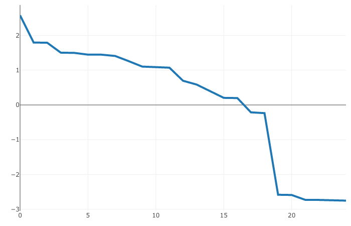
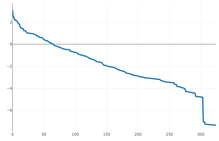
We next proceed to equations of degree $2$. Our hope is to find the $16$ quadrics in (24). Let us check whether this works. Figure 12 on the right shows the logarithms of the singular values of the multivariate Vandermonde matrix $U_{\leq 2}(\Omega)$. Based on this we set $\tau=10^{-6}$.

The command FindEquations(M, :with_svd, 2, 1e-6) reveals $21$ quadrics. However, these are the pairwise products of the $6$ linear equations we found earlier. An explanation for why we cannot find the $16$ distance quadrics is as follows. Each of the $6$ linear equations evaluated at the points in $\Omega$ gives about $10^{-3}$ in our numerical computations. Thus their products equal about $10^{-6}$. The distance quadrics equal about $10^{-3}$. At tolerance $10^{-6}$, we miss them. Their values are much larger than the $10^{-6}$ from the $21$ redundant quadrics. By randomly rotating and translating each data point, we can manipulate the dataset such that FindEquations together with a tolerance value $\tau=10^{-1}$ gives the $16$ desired quadrics. The fact that no linear equation vanishes on the manipulated dataset provides more evidence that 3 linear equations are determining the normal form for rotations.

Figure 13: Barcodes for a subsample of 500 points from the cyclo-octane dataset. The left plot shows the barcodes for the usual Vietoris-Rips complex. The right picture shows barcodes for the ellipsoid-driven simplicial complex in (17). The right barcode correctly captures the homology of the conformation space.

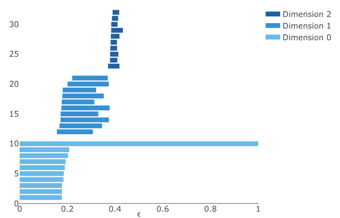
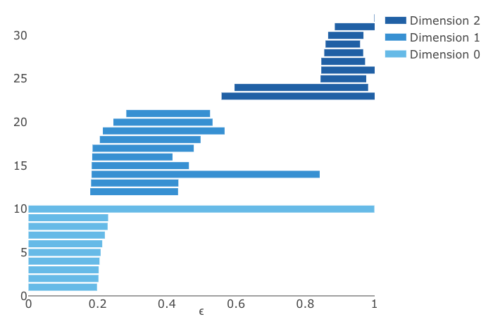
The cyclo-octane dataset was used in [3, §.6.3] to demonstrate that persistent homology can efficiently recover the homology groups of the conformation space. We confirmed this result using our software. We determined the barcodes for a random subsample of 500 points. In addition to computing with Vietoris-Rips complexes, we use the 6 linear equations and the 16 distance quadrics to produce the ellipsoid-driven barcode plots. The results are displayed in Figure 13. The barcodes from the usual Vietoris-Rips complex do not capture the correct homology groups, whereas the barcodes arising from our new complex (17) do.

Acknowledgements. We thank Henry Adams, Mateo Díaz, Jon Hauenstein, Peter Hintz, Ezra Miller, Steve Oudot, Benjamin Schweinhart, Elchanan Solomon, and Mauricio Velasco for helpful discussions. Bernd Sturmfels and Madeleine Weinstein acknowledge support from the US National Science Foundation.

Authors’ addresses:

Paul Breiding,  MPI-MiS Leipzig Paul.Breiding@mis.mpg.de

Sara Kališnik,  MPI-MiS Leipzig and Wesleyan University skalisnikver@wesleyan.edu

Bernd Sturmfels,   MPI-MiS Leipzig and UC Berkeley bernd@mis.mpg.de

Madeleine Weinstein, UC Berkeley maddie@math.berkeley.edu

References

- [1]
- [2] E. Aamari, J. Kim, F. Chazal, B. Michel, A. Rinaldo and L. Wasserman: Estimating the reach of a manifold, arXiv:1705.04565.
- [3] H. Adams and A. Tausz: JavaPlex Tutorial, http://www.math.colostate.edu/~adams/research/javaplex_tutorial.pdf, 24.2.2018.
- [4] C. Améndola, J.-C. Faugère and B. Sturmfels: Moment varieties of Gaussian mixtures, Journal of Algebraic Statistics 7 (2016) 14-28.
- [5] R. Basson, R. Lercier, C. Ritzenthaler and J. Sijsling: An explicit expression of the Lüroth invariant, ISSAC 2013, Proceedings of the 38th International Symposium on Symbolic and Algebraic Computation, 31–36, ACM, New York, 2013.
- [6] D. Bates, J. Hauenstein, A. Sommese and C. Wampler: Numerically Solving Polynomial Systems with Bertini, Software, Environments, and Tools, SIAM, Philadelphia, PA, 2013.
- [7] J. Bezanson, A. Edelman, S. Karpinski and V. Shah: Julia: A fresh approach to numerical computing, SIAM Review 59 (2017) 65–98.
- [8] A. Bjoerck and V. Pereyra: Solutions of Vandermonde systems of equations, Mathematics of Computation 24 (1970) 893–903.
- [9] G. Blekherman, P. Parrilo and R. Thomas: Semidefinite Optimization and Convex Algebraic Geometry, MOS-SIAM Series on Optimization 13, 2012.
- [10] P. Breiding and S. Timme: HomotopyContinuation.jl - a package for solving systems of polynomial equations in Julia, arXiv:1711.10911.
- [11] M.W. Brown, S. Martin, S.N. Pollock, E.A. Coutsias and J.P.Watson: Algorithmic dimensionality reduction for molecular structure analysis, Journal of Chemical Physics, 129 (2008) 064118.
- [12] P. Bürgisser, F. Cucker and P. Lairez: Computing the homology of basic semialgebraic sets in weak exponential time, arXiv:1706.07473.
- [13] F. Camastra: Data dimensionality estimation methods: a survey, Pattern Recognition 36 (2003) 2945–2954.
- [14] F. Camastra and A. Staiano: Intrinsic dimension estimation: Advances and open problems, Information Sciences 328 (2016) 26–41.
- [15] G. Carlsson: Topology and data, Bull. Amer. Math. Soc. 46 (2009) 255-308.
- [16] D. Cifuentes and P. Parrilo: Sampling algebraic varieties for sum of squares programs, SIAM Journal on Optimization 27 (2017) 2381–2404.
- [17] D. Cox, J. Little and D. O’Shea: Ideals, Varieties, and Algorithms: An Introduction to Computational Algebraic Geometry and Commutative Algebra, 4th ed., Undergrad. Texts in Math., Springer, 2015.
- [18] M.A. Cueto, J. Morton and B. Sturmfels: Geometry of the restricted Boltzmann machine, Algebraic Methods in Statistics and Probability, 135–153, Contemp. Math. 516, AMS, Providence, 2010.
- [19] N. Daleo and J. Hauenstein: Numerically deciding the arithmetically Cohen-Macaulayness of a projective scheme, J. Symbolic Computation 72 (2016) 128–146.
- [20] J. W. Demmel: Applied Numerical Linear Algebra, SIAM, Philadelphia, 1997.
- [21] M. Deza and M. Laurent: Geometry of Cuts and Metrics, Algorithms and Combinatorics 15, Springer-Verlag, Berlin, 1997.
- [22] P. Diaconis, S. Holmes and M. Shahshahani: Sampling from a manifold, Institute of Mathematical Statistics Collections 10 (2013) 102–125.
- [23] M. Díaz, A. Quiroz and M. Velasco: Local angles and dimension estimation from data on manifolds, arXiv:1805.01577.
- [24] J. Draisma, E. Horobeţ, G. Ottaviani, B. Sturmfels and R. Thomas: The Euclidean distance degree of an algebraic variety, Found. Comput. Math. 16 (2016) 99–149.
- [25] M. Drton, B. Sturmfels and S. Sullivant: Lectures on Algebraic Statistics, Oberwolfach Seminars, 39, Birkhäuser Verlag, Basel, 2009.
- [26] E. Dufresne, P. Edwards, H. Harrington and J. Hauenstein: Sampling real algebraic varieties for topological data analysis, arXiv:1802.07716.
- [27] D. Eklund: The numerical algebraic geometry of bottlenecks, arXiv:1804.01015.
- [28] H. Federer: Curvature measures, Trans. Amer. Math. Soc. 93 (1959) 418-491.
- [29] Z. Griffin, J. Hauenstein, C. Peterson and A. Sommese: Numerical computation of the Hilbert function and regularity of a zero dimensional scheme, Connections between Algebra, Combinatorics, and Geometry, 235–250, Springer Proc. Math. Stat. 76, Springer, New York, 2014.
- [30] J. Harris: Algebraic Geometry. A First Course, Graduate Texts in Mathematics 133, Springer-Verlag, New York, 1992.
-
[31]
G. Henselman and R. Ghrist:
Matroid filtrations and computational persistent homology,
arXiv:1606.00199. - [32] N. Higham: Accuracy and Stability of Numerical Algorithms, SIAM, 2nd edition, 2002.
- [33] E. Horobeţ and M. Weinstein: Offset hypersurfaces and persistent homology of algebraic varieties, arXiv:1803.07281.
- [34] R. Howard: The kinematic formula in Riemannian homogeneous spaces, Mem. Amer. Math. Soc. 106 (509) (1993).
- [35] A. Jain and R. Dubes: Algorithms for Clustering Data, Prentice-Hall, Upper Saddle River, NJ, 1998.
- [36] J. Kileel, Z. Kukelova, T. Pajdla and B. Sturmfels: Distortion varieties, Found. Comput. Math. (2018).
- [37] M. Kummer and C. Vinzant: The Chow form of a reciprocal linear space, Michigan Math. Journal, to appear, arXiv:1610.04584.
- [38] J.M. Landsberg: Tensors: Geometry and Applications, Graduate Studies in Mathematics 128, American Mathematical Society, Providence, RI, 2012.
- [39] J.A. Lee and M. Verleysen: Nonlinear Dimensionality Reduction, Information Science and Statistics, Springer Verlag, New York, 2007.
- [40] K. Leichtweiss: Zur Riemannschen Geometrie in Grassmannschen Mannigfaltigkeiten, Mathematische Zeitschrift 76 (1961) 334–366.
- [41] E. Levina and P. Bickel: Maximum likelihood estimation of intrinsic dimension, Advances in Neural Information Processing Systems 17 (2004) 777–784.
- [42] Y. Ma, A. Yang, H. Derksen and R. Fossum: Estimation of subspace arrangements with applications in modeling and segmenting mixed data, SIAM Review 50 (2008) 413–458.
- [43] S. Martin, A. Thompson, E. A. Coutsias, and J. P. Watson: Topology of cyclo-octane energy landscape, Journal of Chemical Physics 132 (2010) 234115.
- [44] F. Mezzadri: How to generate matrices from the classical compact groups, Notices of the AMS 54 (2007) 592–604.
- [45] H. Möller and B. Buchberger: The construction of multivariate polynomials with preassigned zeros, Computer Algebra (Marseille 1982), 24–31, Lecture Notes in Computer Science 144, Springer, Berlin, 1982.
- [46] M. Mustaţǎ: Graded Betti numbers of general finite subsets of points on projective varieties, Pragmatic 1997, Matematiche (Catania) 53 (1998) 53–81.
- [47] P. Niyogi, S. Smale and S. Weinberger: Finding the homology of submanifolds with high confidence from random samples, Discrete Comput. Geometry 39 (2008) 419–441.
- [48] P. J. Olver: On multivariate interpolation, Studies in Appl. Math. 116 (2006) 201–240.
- [49] V. Y. Pan: How bad are Vandermonde matrices?, SIAM J. Matrix Anal. & Appl. 37(2) (2016) 676–694.
- [50] The Pattern Analysis Lab at Colorado State University: A fractal dimension for measures via persistent homology, Preprint, 2018.
- [51] D. Plaumann, B. Sturmfels and C. Vinzant: Quartic curves and their bitangents, Journal of Symbolic Computation 46 (2011) 712–733.
- [52] L. Santalo: Integral Geometry and Geometric Probability, Addison-Wesley, 1976.
- [53] B. Sturmfels and V. Welker: Commutative algebra of statistical ranking, J. Algebra 361 (2012) 264–286.