Self Super-Resolution for Magnetic Resonance Images using Deep Networks

Abstract

High resolution magnetic resonance (MR) imaging (MRI) is desirable in many clinical applications; however, there is a trade-off between resolution, speed of acquisition, and noise. It is common for MR images to have worse through-plane resolution (slice thickness) than in-plane resolution. In these MRI images, high frequency information in the through-plane direction is not acquired, and cannot be resolved through interpolation. To address this issue, super-resolution methods have been developed to enhance spatial resolution. As an ill-posed problem, state-of-the-art super-resolution methods rely on the presence of external/training atlases to learn the transform from low resolution (LR) images to high resolution (HR) images. For several reasons, such HR atlas images are often not available for MRI sequences. This paper presents a self super-resolution (SSR) algorithm, which does not use any external atlas images, yet can still resolve HR images only reliant on the acquired LR image. We use a blurred version of the input image to create training data for a state-of-the-art super-resolution deep network. The trained network is applied to the original input image to estimate the HR image. Our SSR result shows a significant improvement on through-plane resolution compared to competing SSR methods.

Index Terms—  self super-resolution, deep network, MRI, CNN

1 Introduction

The spatial resolution of magnetic resonance (MR) images (MRI) is chosen based on imaging time, desired signal to noise ratio, and other factors. Ultimately, the spatial resolution is limited by the amount of $k$-space acquired in the Fourier domain. To facilitate faster, and therefore cheaper, MRI acquisitions, it is common for MR images to have worse through-plane resolution (slice thickness) than in-plane resolution. This means that the in-plane data has a relatively complete sampling of $k$-space along an appropriate axis, whereas data in the through-plane direction is bandlimited within the corresponding $k$-space.

One common way to address the resolution mismatch between the in-plane and through-plane directions is to upsample the data to an isotropic resolution. This, however, results in images with partial volume artifacts that lead to degraded image analysis in subsequent processing. More appropriate approaches for estimating the high frequency information are known as super-resolution (SR) methods, as they are meant to enhance the spatial resolution. SR has been a well-explored technique in computer vision. Popular methods include neighbor embedding regression [1, 2], random forest approaches [3, 4], and state-of-the-art CNN methods such as those reported for the NTIRE 2017 Challenge [5], most of which were based on VDSR [6] or SRResNet [7] as a baseline model. EDSR [8] which was modified from SRResNet [7] had the best performance in the NTIRE 2017 Challenge.

Unfortunately, all the NTIRE 2017 Challenge methods require external paired atlas images to learn the transformation from low (LR) to high resolution (HR). This is not a desirable situation for MR imaging, as training data is not generally available because: 1) scanner gain means that even data acquired on the same scanner will have a different dynamic range; 2) acquiring HR MR data is difficult due to scan times, patient motion and safety; and 3) it is difficult to match atlas and subject image resolutions perfectly. In contrast, exsiting single image self super-resolution (SSR) methods [9, 10, 11] downsample the LR image to create a lower resolution (LR₂) image and learn the mapping from LR₂ to LR; and subsequently apply the mapping to LR with the goal of approximating HR.

In this paper, we build upon the work of Jog et al. [11] which had an alternative approach to SSR. Jog et al. used the fact that MR images are inherently anisotropic to learn a regression between LR and HR images. The approach generated new additional images, each of which is LR along a certain direction, but is HR in the plane normal to it. Thus, each new image contributed information to a new region of Fourier space. Then the collection of images is combined using Fourier Burst Accumulation [12]. We modify the deep network framework of EDSR [8], while incorporating the ideas of Jog et al. to provide the training data. Thus, we present a single image SSR deep network framework for MR images. We refer to it as EDSSR.

2 Method

Consider an HR image $I(x,y,z)$ reconstructed from its $k$-space signal $F(u,v,w)$. To save acquisition time and to improve signal-to-noise ratio, $F(u,v,w)$ is bandlimited along the $w$-axis. The missing portion of $k$-space is filled with $0$ and we refer to this Fourier space as $F_{w}(u,v,w)$, with the reconstructed image denoted as $I_{z}(x,y,z)$. $I_{z}(x,y,z)$ has the same digital resolution as $I(x,y,z)$, and has low spatial resolution in the $z$ direction. The goal is to restore $I(x,y,z)$ from $I_{z}(x,y,z)$ without any external training data.

Fig. 1: The framework of our algorithm.

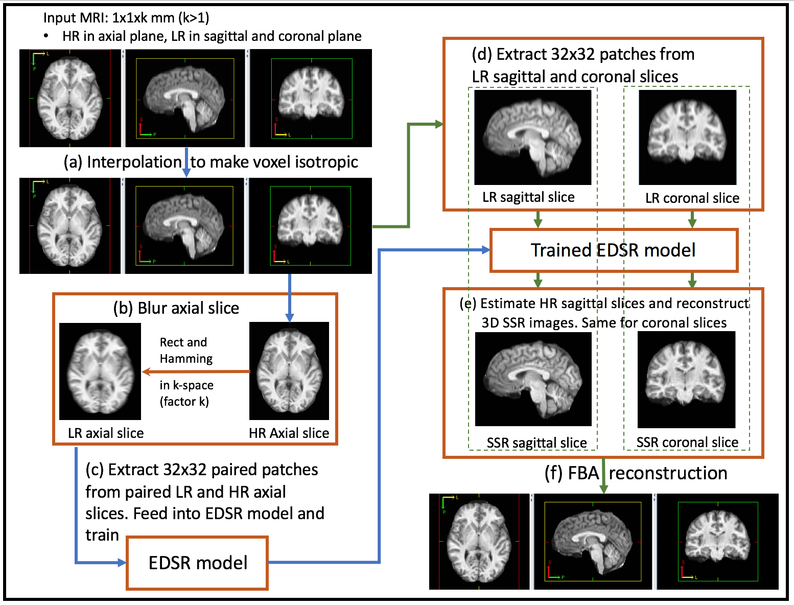An overview of our framework is provided in Fig. 1. Given a LR input image $I_{z}(x,y,z)$ with digital resolution $1\times 1\times k$ where $k>1$, we know that it has isotropic digital resolution in the $xy$-plane, and low resolution in the $z$-axis, i.e. its axial slices have high resolution $1\times 1$, while sagittal and coronal slices have low resolution $k\times 1$. We first use interpolation to make the volume isotropic; we use zero-padding in $k$-space though alternatives like cubic spline interpolation (BSP) may also be used. As the high frequency information in $F_{w}(u,v,w)$ is completely missing, this interpolation does not improve the spatial resolution. Instead, we need a non-linear model to estimate the HR image from the LR image. State-of-the-art SR models using deep networks (EDSR [5]) use paired HR and LR training data. However, in our setting, no external training data is available.

To circumvent the lack of training data, we simulate training data from the input image $I_{z}(x,y,z)$. To do this, we note that each 2D axial slice $I_{z}(x,y)$ in $I_{z}(x,y,z)$ is actually an HR image, while each coronal slice $I_{z}(x,z)$ and each sagittal slice $I_{z}(y,z)$ are LR images. By blurring $I_{z}(x,y,z)$ along the $x$-axis, we can obtain a LR image in both the $x$ and $z$ directions, which we denote as $I_{zx}(x,y,z)$. The blurred image $I_{zx}(x,y,z)$ and input image $I_{z}(x,y,z)$ are used as our training data. The axial slices $I_{zx}(x,y)$ of $I_{zx}(x,y,z)$ have resolution of $k\times 1$, while the axial slices $I_{z}(x,y)$ of $I_{z}(x,y,z)$ have resolution of $1\times 1$. Now, if we can learn a mapping from LR image $I_{zx}(x,y)$ to HR image $I_{z}(x,y)$, we can apply the mapping to LR images $I_{z}(x,z)$ and $I_{z}(y,z)$ to estimate the HR images $I(x,z)$ and $I(y,z)$.

We use EDSR, a state-of-the-art deep network SR model, to learn the transformation. After applying the trained model to coronal slices, $I_{z}(x,z)$, we get $\hat{I}^{y}(x,z)$, an estimate of $I(x,z)$. By stacking together each $\hat{I}^{y}(x,z)$, we have $\hat{I}^{y}(x,y,z)$. We can repeat this process for $I_{z}(y,z)$ to generate $\hat{I}^{x}(y,z)$ and subsequently $\hat{I}^{x}(x,y,z)$. Similar to Jog et al. [11], we use Fourier Burst Accumulation (FBA) [12] to reconstruct $\hat{I}(x,y,z)$ from the two images $\hat{I}^{y}(x,y,z)$ and $\hat{I}^{x}(x,y,z)$. Complete details of the construction of the training data and our modifications to EDSR are listed below.

Training data extraction: We first blur $I_{z}(x,y,z)$ in the $x$-axis and obtain $I_{zx}(x,y,z)$. To simulate the data acquisition process in MRI, we use the low pass filter on the $k$-space signal $F_{w}(u,v,w)$. A rect function on the $u$-axis is multiplied with $F_{w}(u,v,w)$, generating $F_{wu}(u,v,w)$ while guaranteeing no high frequency information on the $u$-axis. For 3D acquired MR images, a window function might be applied along the $w$-axis during reconstruction to avoid ringing. To increase the amount of available training data, we use rotated versions of the original image. If we rotate $I_{z}(x,y,z)$ in the $xy$-plane, the rotated images $R_{xy}(\theta)\circ I_{z}(x,y,z)$ still has resolution $1\times 1\times k$. We can therefore do the same blurring to the rotated images $R_{xy}(\theta)\circ I_{z}(x,y,z)$ to obtain more training data. We randomly extract $32\times 32$ patches in each slice $z$ of $I_{zx}(x,y,z)$ and it matching pair in $I_{z}(x,y,z)$, as well as from the rotated images; feeding these paired 2D HR and LR patches into the deep network to train it.

EDSR model: We use the default number of layers and loss as in the original EDSR [5] except for one modification. The original EDSR [5] framework used an upsampling layer in the model to make the image pixels isotropic. We in contrast upsample the LR image to an isotropic resolution prior to being input into the deep network, thus there is no upsampling layer in the model. A reason for this, is the upsampling factor $k$ varies among different data sets. By having this factor be part of the network would force the model to be changed and thus retrained for each new data set. By having a fixed network structure and doing the isotropic resampling outside the EDSR framework, allows the network weights to be reused between data sets with only fine-tune of the pre-trained network weights. This modification can cut the time cost by approximately $50$-$90\%$ depending on the similarity between the current data set and the pre-trained data set. An additional benefit being that EDSR required the factor $k$ to be an integer which is generally not true of MR images, however our framework allows $k$ to be a non-integer value.

3 Experiments

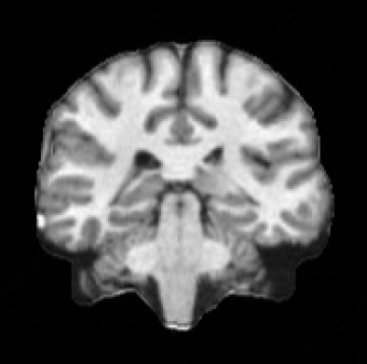
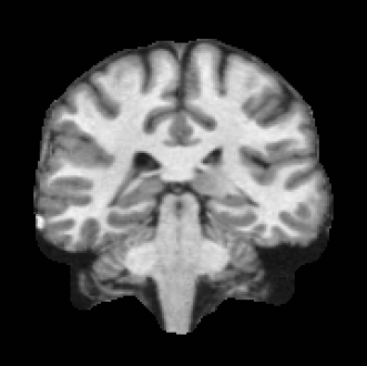
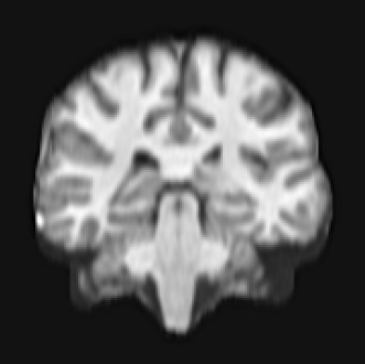
We ran our algorithm on $T_{1}$-weighted Magnetization Prepared Rapid Gradient Echo (MPRAGE) images from 20 subjects of the Neuromorphometrics dataset, and compare with other methods. The ground truth HR image has a resolution of $1\times 1\times 1$ mm. As the input of SSR algorithms, the LR images are simulated by downsampling in the $z$-axis from the ground-truth HR image by a factor $k$ of 2 and 3. Cubic B-spline interpolation (BSP) and SSR [11], as well as our method are shown for the downsampling factors of 2 and 3 in Fig. 2 and Fig. 3, respectively. Visually, our EDSSR approach can significantly improve through-plane resolution compared to BSP and SSR [11], especially in Fig. 3 when the downsampling scale factor is 3. A comparison of the PSNR values for the three methods is shown in Table 1, with the SSIM for all three methods being shown in Table 2. The ‘*’ indicates that the results are statistically significantly greater than all the methods using a one-tailed t-test and Wilcoxon rank-sum tests. Our EDSSR approach shows superiority in SSIM and PSNR for input LR images with resolution of $1\times 1\times 3$mm.

(a) BSP ($k=2$)

(b) SSR ($k=2$) [11]

(c) EDSSR ($k=2$)

(d) HR (1mm)

Fig. 2: Coronal views of the (a) cubic B-spline (BSP) interpolated image of the 2 mm LR image, (b) result using SSR [11], (c) our result EDSSR using EDSR and FBA, (d) HR ground truth image

(a) BSP ($k=3$)

(b) SSR ($k=3$) [11]

(c) EDSSR ($k=3$)

(d) HR (1mm)

Fig. 3: Coronal views of the (a) cubic B-spline (BSP) interpolated image of the 3 mm LR image, (b) result using SSR [11], (c) our result EDSSR using EDSR and FBA, (d) HR ground truth image

Table 1: Mean PSNR values (dB) for 20 subjects. The ‘*’ indicates that the results are statistically significantly greater than all the methods using a one-tailed t-test and Wilcoxon rank-sum tests for the PSNR metric.

LR		BSP		SSR		EDSSR
2mm		35.99		37.98*		35.14
3mm		31.98		33.49		34.44*

Table 2: Mean SSIM values for 20 subjects. The ‘*’ indicates that the results are statistically significantly greater than all the methods using a one-tailed t-test and Wilcoxon rank-sum tests for the SSIM metric.

LR		BSP		SSR		EDSSR
2mm		0.9873*		0.9832		0.9763
3mm		0.9635		0.9678		0.9773*

(a) BSP

(b) SSR [11]

(c) EDSSR

(d) BSP

(e) SSR[11]

(f) EDSSR

Fig. 4: Coronal views of the (a) cubic B-spline (BSP) interpolated image of the $0.83\times 0.83\times 2.20$ mm LR image, (b) result using ANR and FBA [11], (c) our result using EDSR and FBA; zoomed images of the (d) BSP interpolated image, (e) result using ANR and FBA [11], (f) our result using EDSR and FBA,

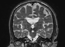
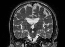
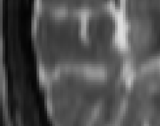
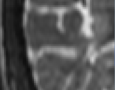
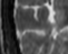
We also experimented using real LR image data. We used T2-weighted MRI acquired at $1.14\times 1.14\times 2.20$ mm in 2D, and reconstructed at $0.83\times 0.83\times 2.20$ mm, with the scale factor being $k=2.20/0.83\approx 2.65$. The results for our method and SSR are shown in Fig. 4. The lower row shows a zoom on an edge. Although there is no ground truth, visually our approach gives significantly better results than BSP and SSR [11].

4 Conclusion and Discussion

This paper presents an SSR approach which does not need any external training data to estimate an HR image from a LR image. It uses patches in blurred axial slices of the image itself to create paired training data, and the state-of-the-art SR model from EDSR to model the mapping from LR patches to HR patches. Finally, it uses FBA [12] to reconstruct the final image, taking advantage of SR results from different orientations. The results are significantly better than competing methods, in particular with decreasing through-plane resolution (ie. increasing slice thickness).

Deep networks are known to be dependent on “good” atlas data. The variance between atlas and subject could cause severe over-fitting. However, real-world MR images have relatively varying intensities. This SSR algorithm not only fits in the clinical practice that the MR images with high through-plane resolution are usually unavailable, but also guarantees the intensity invariance between atlas and subject, which reduces the over-fitting of the deep network. In summary, this SR algorithm can improve image resolution without any external data.

References

- [1] H. Chang, D.-Y. Yeung, and Y. Xiong, “Super-resolution through neighbor embedding,” in Computer Vision and Pattern Recognition, 2004. CVPR 2004. Proceedings of the 2004 IEEE Computer Society Conference on. IEEE, 2004, vol. 1, pp. I–I.
- [2] R. Timofte, V. De Smet, and L. Van Gool, “A+: Adjusted anchored neighborhood regression for fast super-resolution,” in Asian Conference on Computer Vision. Springer, 2014, pp. 111–126.
- [3] S. Schulter, C. Leistner, and H. Bischof, “Fast and accurate image upscaling with super-resolution forests,” in Proceedings of the IEEE Conference on Computer Vision and Pattern Recognition, 2015, pp. 3791–3799.
- [4] J. Salvador and E. Pérez-Pellitero, “Naive bayes super-resolution forest,” in Proceedings of the IEEE International Conference on Computer Vision, 2015, pp. 325–333.
- [5] R. Timofte, E. Agustsson, L. Van Gool, M.-H. Yang, L. Zhang, B. Lim, S. Son, H. Kim, S. Nah, K.M. Lee, et al., “Ntire 2017 challenge on single image super-resolution: Methods and results,” in Computer Vision and Pattern Recognition Workshops (CVPRW), 2017 IEEE Conference on. IEEE, 2017, pp. 1110–1121.
- [6] J. Kim, J. Kwon Lee, and K.M. Lee, “Accurate image super-resolution using very deep convolutional networks,” in Proceedings of the IEEE Conference on Computer Vision and Pattern Recognition, 2016, pp. 1646–1654.
- [7] C. Ledig, L. Theis, F. Huszár, J. Caballero, A. Cunningham, A. Acosta, A. Aitken, A. Tejani, J. Totz, Z. Wang, et al., “Photo-realistic single image super-resolution using a generative adversarial network,” arXiv preprint arXiv:1609.04802, 2016.
- [8] B. Lim, S. Son, H. Kim, S. Nah, and K.M. Lee, “Enhanced deep residual networks for single image super-resolution,” in The IEEE Conference on Computer Vision and Pattern Recognition (CVPR) Workshops, 2017.
- [9] J.-B. Huang, A. Singh, and N. Ahuja, “Single Image Super-Resolution From Transformed Self-Exemplars,” in The IEEE Conference on Computer Vision and Pattern Recognition (CVPR), June 2015.
- [10] Martin Weigert, Loic Royer, Florian Jug, and Gene Myers, “Isotropic reconstruction of 3d fluorescence microscopy images using convolutional neural networks,” arXiv preprint arXiv:1704.01510, 2017.
- [11] A. Jog, A. Carass, and J.L Prince, “Self super-resolution for magnetic resonance images,” in International Conference on Medical Image Computing and Computer-Assisted Intervention. Springer, 2016, pp. 553–560.
- [12] M. Delbracio and G. Sapiro, “Hand-Held Video Deblurring Via Efficient Fourier Aggregation,” IEEE Transactions on Computational Imaging, vol. 1, no. 4, pp. 270–283, 2015.