Depth Masked Discriminative Correlation Filter

Abstract

Depth information provides a strong cue for occlusion detection and handling, but has been largely omitted in generic object tracking until recently due to lack of suitable benchmark datasets and applications. In this work, we propose a Depth Masked Discriminative Correlation Filter (DM-DCF) which adopts novel depth segmentation based occlusion detection that stops correlation filter updating and depth masking which adaptively adjusts the spatial support for correlation filter. In Princeton RGBD Tracking Benchmark, our DM-DCF is among the state-of-the-art in overall ranking and the winner on multiple categories. Moreover, since it is based on DCF, “DM-DCF” runs an order of magnitude faster than its competitors making it suitable for time constrained applications.

I Introduction

Generic short-term object tracking has been a popular research topic in computer vision for the last few years and trackers based on the Discriminative Correlation Filter (DCF) [12] have been particularly successful for applications with time constraint [24, 11, 7, 15]. However, in RGB tracking, there are fundamental difficulties that can be solved with the help of depth (D) information, occlusion handling being the most obvious. Additionally, RGBD sensors are popular in robotics where 3D object tracking also has many important applications, e.g., object manipulation and grasping.

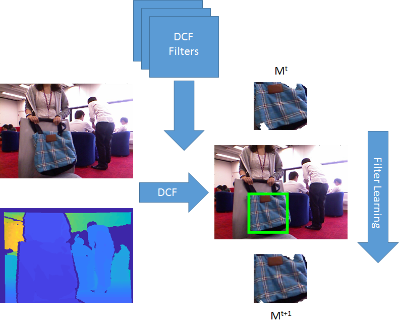
Figure 1: Overview of our DM-DCF method. Depth cue is used in parallel with DCF tracking by inherently adopting depth based masks into DCF formulation which allows altering the filter supports. Moreover, combination of DCF and depth segmentation mitigates the possible errors stemming from individual observations. ($M^{t}$ and $M^{t+1}$ are the masks used for filter training where the slight differences between the masks of two consecutive frames are visible)

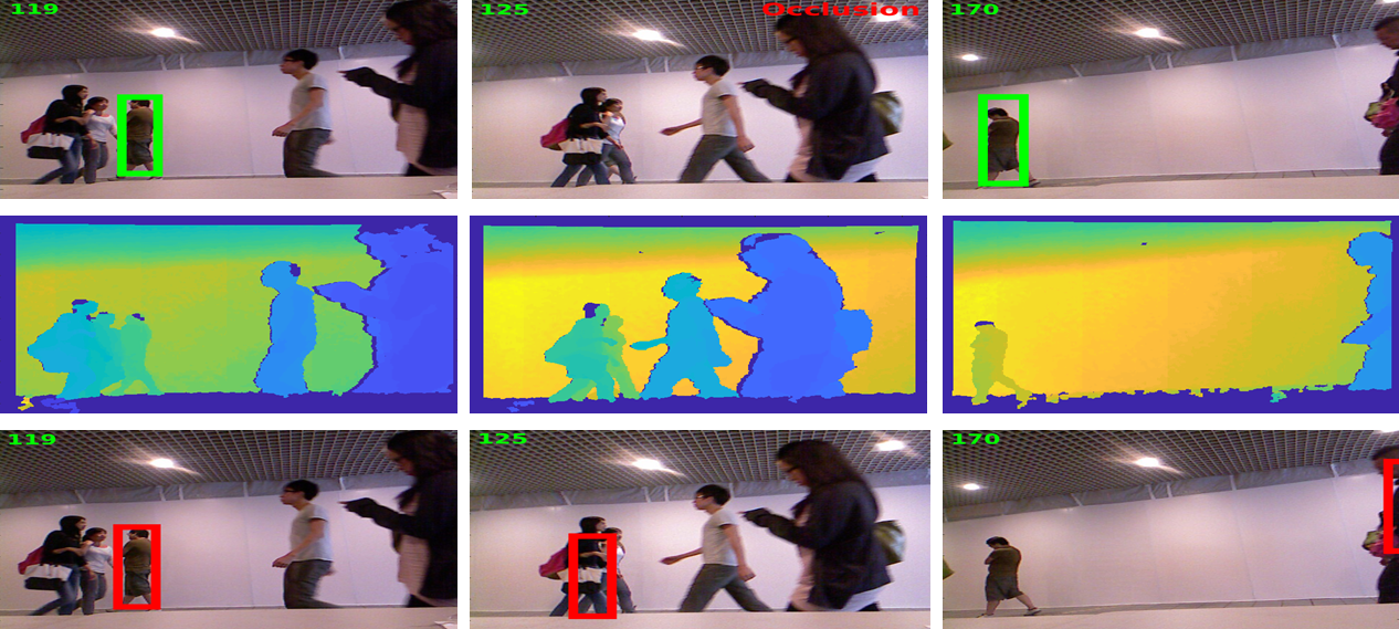
Figure 2: Example results of our DM-DCF tracker (top row) that uses depth cue (middle row) to construct depth masks. Depth helps detecting occlusions as the third dimension provides a strong clue and hence, the tracker stops updating the object model. However, RGB tracker (CSR-DCF [15], bottom row) is not able to detect the occlusions and continues learning occluding object and consequently, loses the target object.

There have been surprisingly small number of works on RGBD tracking since the introduction of the first dedicated benchmark for RGBD tracking: Princeton RGBD Tracking dataset [21]. The dataset authors also proposed baseline trackers for 2D (depth as an additional cue) and 3D tracking (3D bounding box). More recently, particle filter based methods have been proposed by Meshgi et al.  [16] and Bibi et al.  [2], but they are both slow for real-time applications. Instead, we adopt the Discriminative Correlation Filter (DCF) approach since it is proven to be fast and successful in RGB tracking. The two other DCF based RGBD works to our best knowledge are Hannuna et al. [10] and An et al. [1] which are both among the top performers in the Princeton dataset.

In aforementioned RGBD tracking methods, depth has been used as a mere additional cue for tracking, but intuitively the most important role for the depth information is in accurate and robust occlusion handling. In our work, instead of separating occlusion handling and tracking, we unite the two processes by integrating occlusion handling with correlation filters in the sense that the spatial filter supports are dynamically altered using the depth based segmentation. In this work we make the following novel contributions:

• We propose a novel occlusion handling mechanism based on object’s depth distribution and DCF’s response history. By detecting strong occlusions, our tracker avoids corrupting the object model.

• We propose depth masking for DCF which avoids using the occluded regions in matching and therefore provides more reliable tracking scores.

• We experimentally validate Depth Masked Discriminative Correlation Filter (DM-DCF) tracker on the Princeton RGBD Tracking benchmark where it ranks among the state-of-the-art algorithms with ranking first in multiple categories while being faster than the other top performing methods in the benchmark.

Our code will be made publicly available to facilitate fair comparisons.

II Related Work

Object Tracking – Existing trackers for generic short-term object tracking on RGB videos can be grouped under two main categories, Generative (matching with updated target model) or Discriminative (classifier based) methods, depending on how a tracked object (target region) is modelled and localized [20]. A generative tracker represents the target as a collection of features from previously tracked frames and matches them to search region in the current frame. A few prominent examples of this family of trackers are Incremental Visual Tracking (IVT) [19], Structural Sparse Tracking (SST) [23] and kernel-based object tracking (mean shift) [5]. Generative trackers build a model from the positive examples, e.g. tracked regions, but false matches occur if the background or other objects have similar texture properties. This issue is addressed in discriminative trackers by continuously learning and updating a classifier that distinguishes the target from background. In recent years, discriminative approach has been more popular and it has produced many well-performing trackers such as Tracking-Learning-Detection (TLD) [13], Continuous Convolutional Operators Tracking (C-COT) [8], Multi-Domain Convolutional Neural Network (MDNet) [17], ECO [7], CSR-DCF [15]. Due to its mathematical simplicity, efficiency and superior performance, we adopted the DCF based approach as our baseline to allow us to achieve fast throughput rate while retaining an accuracy comparable to more complicated algorithms as it is proven in VOT 2017 [24].

Object Tracking with Depth – The number of research papers on generic RGBD (color + depth) object tracking is surprisingly limited despite the fact that depth sensors are ubiquitous and the apparent application of the problem in robotics. One of the reasons is the lack of suitable datasets until recent years. In 2013 Song et al.  [21] introduced the Princeton Dataset for RGBD tracking and nine variations of a baseline tracker. They presented two main approaches; depth as an additional cue and point cloud tracking. In the first case, depth is added as an additional dimension to Histogram of Oriented Gradients (HOG) feature space and in the second case tracking is based on 3D point clouds producing also a 3D bounding box. Their best method performs well, but contains heuristic processing stages and its speed (0.26 FPS) makes the algorithm unsuitable for real-time applications.

Another RGBD method was recently proposed by Meshgi et al.  [16] who tackled the problem with an occlusion-aware particle filter framework employing a probabilistic model. Although their algorithm is among the top performers on Princeton Benchmark, the complexity of their model, the number of parameters to be tuned and the slowness of the algorithm (0.9 FPS) makes it unpractical for many applications.

Bibi et al.  [2] suggested a part-based sparse tracker within a particle filter framework. They represented particles as 3D cuboids that consist of sparse linear combination of dictionary elements which are not updated over the time. In case of no occlusion, their method first finds a rough estimate of the target location using 2D optical flow. Following this, particles are sampled in rotation $\boldsymbol{R}$ and translation $\boldsymbol{T}$ space. To detect the occlusions, they adopted a heuristic which states that the number of points in the 3D cuboid of the target should decrease below a threshold. Their method sets currently the state-of-the-art on Princeton benchmark however, computation times are not mentioned in the original work.

To the authors’ best knowledge there are only two RGBD trackers based on DCF which is used in our method. The first one was proposed by Hannuna et al.  [10] who use depth for occlusion handling, scale and shape analysis. To this end, they first apply a clustering scheme on depth histogram which is followed by formation of a single Gaussian distribution based depth modelling where they assume the cluster with the smallest mean must be the object (similar heuristic used in Song et al.  [21]). Another shortcoming of their algorithm is that their occlusion handling allows tracking of occluding region which introduces same problems as in [21].

Second method was proposed by An et al.  [1]. They used depth based segmentation in parallel to Kernelized Correlation Filter (KCF) [11] detection and then interpreted the results to locate the target and determine the occlusion state with a heuristic approach.

The rest of the paper is organized as follows; Section III provides an overview for the proposed tracking method, Section IV reports the results of our tracker, its comparison against the state-of-the-art RGBD trackers and also discusses the ablation studies to evaluate the impacts of our design choices. Finally Section V sums up our proposed method with remarks for the future work. The overview of the proposed method can be seen in Fig. 1 and Alg. 1.

III Depth Masked DCF

Our approach is inspired by the recent work of Lukezic et al. [15] who robustified standard DCF by introducing filter masks and won VOT 2017 challenge in real-time track. However, their method is plain RGB and our RGBD tracker differs from their work significantly in the following terms. Firstly, their method is an RGB tracker without occlusion handling mechanism. Secondly, we update correlation filter mask using depth cues instead of spatial 2D priors and color segmentation. As we show in Section IV-D, our approach is clearly superior which can be attributed to the power of depth cue.

An overview of our DM-DCF algorithm is given below while Section III-A provides an introduction to DCF based tracking, Section III-B reports how the depth based DCF masks are created, Section III-C discusses the optimization of correlation filters with spatial constraints and Section III-D introduces our occlusion handling mechanism.

Algorithm 1 Depth Masked DCF

0:  Current frame $I^{t}$; Occlusion state $S^{t-1}$; Foreground and background depth distributions $P_{fg}^{t-1}$, $P_{bg}^{t-1}$; Tracker response threshold $\tau$; $K$ last responses $\boldsymbol{r}$

  if $S^{t-1}$ is $false$ then {** Tracker part **}

     Run DCF tracker ($\bf{h}^{t-1}$) on $I^{t}$

     Calculate maximum filter response $r_{max}^{t}$

     Run occlusion detection to obtain $S^{t}$

     Calculate depth mask $\bf{M^{t}}$ (Sec. III-B)

  else {** Detector part **}

     Run full frame detection and obtain $r_{max}^{t}$

     if $r_{max}^{t}>\tau*mean(\boldsymbol{r})$ then

        $S^{t}\leftarrow false$

     else

        $S^{t}\leftarrow true$

     end if

  end if

  if $S^{t}$ is $false$ then {** Mask update part **}

     Update distributions $P_{fg}^{t}$ and $P_{bg}^{t}$ using $\bf{M^{t}}$

     Update $\bf{h}^{t}$ using $\bf{M^{t}}$

     Update tracker response history $\boldsymbol{r}^{mod(t,K)}\leftarrow r_{max}^{t}$

  end if

  Proceed to the next frame

III-A Correlation Filters

The problem to be solved in correlation filter based tracking is to find a suitable filter $h$ at discrete time point $t$ and sample point $i$ that provides desired output $y_{i}$ for given input image $x_{i}$ which includes the target object. Desired output, $y_{i}$, can be constructed by using a small, dense, 2D gaussian at the centre of a tracked object image [3]. Optimization of the filter can be formulated as a ridge regression problem:

$$\frac{1}{2}\sum_{i}||y_{i}-h^{T}x_{i}||^{2}+\frac{\lambda}{2}||h||^{2}$$ (1)

where $\lambda$ is the regularization parameter that is used to avoid overfitting to the current object appearance. A widely used technique is to assume circular repetitions of each input $x_{i}$ as $x_{i}(\Delta\tau_{j})$ where $\Delta\tau_{j}$ represents all circular shifts of $x_{i}$. This assumption leads to a fast filter optimization in the Fourier domain [11]:

$$\hat{h}=\frac{\sum_{i}\hat{x_{i}}^{*}\odot\hat{y_{i}}}{\sum\hat{x_{i}}^{*}\odot\hat{x_{i}}+\lambda}$$ (2)

where $\hat{h}$, $\hat{x}$ and $\hat{y}$ are the Fourier transforms of the correlation filter, input image and the desired output respectively. $\odot$ is the element-wise Hadamar product and ^∗ denotes the Hermitian conjugate. Computation in Fourier domain reduces the complexity from $\mathcal{O}(D^{3}+ND^{2})$ in the spatial domain to $\mathcal{O}(ND\log D)$ for the images of the size $D$ pixels and $N$ examples as it is reported in [9]. However, this also enforces a special form of (1):

$$\frac{1}{2}\sum_{i}\sum_{j}||y_{i}(j)-h^{T}x_{i}(\Delta\tau_{j})||^{2}+\frac{\lambda}{2}||h||^{2}$$ (3)

where $j$ runs over the all $D$ circular shifts of each input $x_{i}$. Henriques et al.  [11] also extended the above to include kernel functions that can make tracker even more effective without any loss in computation speed.

Another important part of correlation filter based tracking is time averaging for online adaptation where previous appearances are retained in “tracker memory” [3]

$$\hat{h}^{t}=\psi\hat{h}^{t}+(1-\psi)\hat{h}^{t-1}$$ (4)

III-B Depth Masking

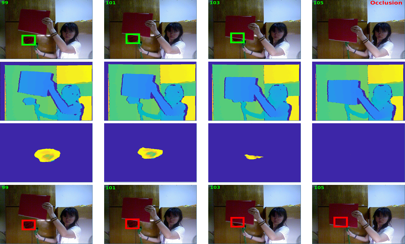
Figure 3: Our method (top) can handle the challenging cases where the state-of-the-art DCF based RGB tracker (CSR-DCF [15]) fails due to the color similarity of a tracked object and back/foreground (bottom). Depth cue (second row) is used to generate a filter mask (third row) which is both used for filter generation and occlusion handling (note detected occlusion in the last frame when detection mode is switched on).

The masking approach in our work to select active pixels (i.e. pixels that are used for DCF updates) for the DCF tracker was inspired by the work of Lukezic et al.  [15] who constructed an RGB cue driven mask by forming a pixel graph where the foreground was segmented by graph cut approach using color histograms and spatial relationships. However, their method is deemed to fail in the cases where background and foreground are of similar color and it cannot detect occlusions as it can be observed in Fig. 2 and Fig. 3. On the other hand, in our method the depth cue turns out to be clearly better in mask generation and also provides an intuitive way to detect occlusion and switching from the tracking to detection mode which provides superior performance in long-term occlusions as in Fig. 2. In the case of foreground masking of a tracked object, the correlation filter is changed to a masked correlation filter, $h_{M}=M\odot h$, which replaces $h$ in (1) or (3). The mask $M$ has value $1$ to mark the visible (active) region of a tracked object and value $0$ to inactivate pixels in the background. Another advantage of masked correlation is the fact that the border effects in cyclic correlation can be removed if the mask is made larger than the current bounding box [9] (up to the size of the whole input frame).

We construct our mask using probabilistic representations $P_{fg}$ and $P_{bg}$ of foreground object and background (note that background in our case means scene elements both closer and further away from the object) respectively. In its simplest form, the mask can be generated from foreground probability ratios

$$M(\boldsymbol{x})=\begin{cases}1,\hbox{if }\frac{P_{fg}}{P_{bg}}>\Omega\\ 0,\hbox{if }\frac{P_{fg}}{P_{bg}}\leq\Omega\\ \end{cases}\enspace$$ (5)

However, we found another approach based on adaptive thresholding to work better since it avoids setting the threshold $\tau$. We assign each mask pixel a probability ratio value $\log{\frac{P_{fg}}{P_{bg}}}$ which produces a “foreground probablity image” and the probability image is thresholded to form a binary foreground mask by the adaptive method of Otsu [18].

For the probability distribution estimation we tested both single Gaussian and Gaussian Mixture Models, but found single Gaussians to perform better and another additional benefit is their fast online update rules. Our distributions are $P_{fg}\propto\mathcal{N}(\mu_{fg},\sigma^{2}_{fg})$ and $P_{bg}\propto\mathcal{N}(\mu_{bg},\sigma^{2}_{bg})$ whose parameters are updated by the following rules:

$$\begin{split}\mu^{(t)}=\mu^{(t)}\theta+(\mu^{(t-1)}(1-\theta))\\ \sigma^{(t)}=\sigma^{(t)}\gamma+(\sigma^{(t-1)}(1-\gamma))\end{split}$$ (6)

where $\theta$ and $\gamma$ are fixed update rates.

To construct the new distribution for the foreground, the depth values that are in the current mask are picked. In the first frame however, the ground truth bounding box provided by the dataset is used to create the initial distributions.

III-C Filter Optimization

A mask generated by the procedure in Section III-B changes the target function (1) to find the optimal correlation filter $h$ into

$$\frac{1}{2}\sum_{i}||y_{i}-h^{T}Mx_{i}||^{2}+\frac{\lambda}{2}||h||^{2}$$ (7)

and the circular function (3) into

$$\frac{1}{2}\sum_{i}\sum_{j}||y_{i}(j)-Mh^{T}x_{i}(\Delta\tau_{j})||^{2}+\frac{\lambda}{2}||h||^{2}$$ (8)

that can be written in the Fourier domain as [9]

$$E(h)=\frac{1}{2}\sum_{i}||\hat{y}_{i}-\hbox{diag}(\hat{x}_{i})^{T}\sqrt{D}\boldsymbol{F}M^{T}h||^{2}+\frac{\lambda}{2}||h||^{2}$$ (9)

where $M^{T}h$ are defined in the spatial domain and $D\boldsymbol{F}$ is the Fourier operator matrix $\boldsymbol{F}$ multiplied by the number of dimensions $D$ in the signal. This solution is very inefficient in the Fourier domain ($\mathcal{O}(D^{3}+ND^{2})$) and therefore the primal solution in the spatial is faster. However, (9) is in the form where the Lagrangian multiplier $\hat{g}$ can be introduced and Alternating Direction Method of Multipliers (ADMM) adopted [4]:

$$\begin{split}&\hbox{minimize }\frac{1}{2}\sum_{i}||\hat{y}_{i}-\hbox{diag}(\hat{x}_{i})^{T}\hat{g}||^{2}+\frac{\lambda}{2}||h||^{2}\\ &\hbox{subject to }\hat{g}=\sqrt{D}\boldsymbol{F}M^{T}h\end{split}\enspace$$ (10)

The augmented Lagrangian method uses the following unconstrained objective

$$\begin{split}&\hbox{minimize }\frac{1}{2}\sum_{i}||\hat{y}_{i}-\hbox{diag}(\hat{x}_{i})^{T}\hat{g}||^{2}+\frac{\lambda}{2}||h||^{2}\\ &+\frac{\mu}{2}\left(\hat{g}-\sqrt{D}\boldsymbol{F}M^{T}h\right)^{2}+\xi\left(\hat{g}-\sqrt{D}\boldsymbol{F}M^{T}h\right)\end{split}$$ (11)

where $\mu$ is the penalty term affecting the convergence and $\xi$ is the Lagrange multiplier updated on each iteration. Optimization iteratively updates the estimates $\hat{g}^{t+1}$ and $h^{t+1}$ and the multiplier using the rule

$$\xi^{t+1}=\xi^{t}-\mu\left(\hat{g}^{t+1}-\sqrt{D}\boldsymbol{F}M^{T}h^{t+1}\right)\enspace$$ (12)

III-D Occlusion Detection

Detecting heavy occlusions ($\geq 90\%$) and consequently stopping model updates is a vital part of occlusion-aware tracking. This process allows DCF to avoid possible model pollution which eventually leads to drifting. In RGB-based DCF, the main source of information for occlusion handling is a correlation filter response at the maximum location $r_{max}$ since a rapid decrease can be considered as an evidence of occlusion [1, 10]. To include tracker based occlusion detection, we calculate running mean of the maximum responses where the maximum of the current frame $r_{max}^{curr}$ is added iteratively:

$$r_{max}^{(t+1)}=r_{max}^{(t)}+\frac{r_{max}^{curr}-r_{max}^{(t)}}{t}\enspace$$ (13)

The main drawback of the above tracker response based occlusion detection is the implicit assumption that occlusions occur faster than model appearance changes. This does not have to be true and might cause false occlusion detections.

To compensate the weakness of filter response based occlusion handling, we introduce a depth cue based occlusion detection which is simple and efficient. Intuitively, all pixels that pass through our probability based mask generation in Section III-B represent depth values where the target object appears. We can easily define the amount of occlusion to be allowed by enforcing a threshold for the visible pixels in $M$ ($10\%$ in all our experiments). This depth based occlusion detection comes without any extra cost since the information is already available from the masking stage.

Our final occlusion detection combines both the filter response based occlusion detection and depth based occlusion detection where an occlusion is declared if both detectors are triggered, i.e. filter response falls below $65\%$ of moving average and number of pixels supporting object depth falls as well below $10\%$ of bounding box regions. If occlusion is detected, the filter update is stopped and the system switches into full image detection mode (occlusion recovery). Occlusion recovery model does not make any assumptions on object’s reappearance probability and it is run as long as the target object is absent in the scene.

IV Experiments

In this section, we present an extensive evaluation of the proposed method. Section IV-A provides implementation details, Section IV-B overviews the dataset and the metrics used for the evaluation, Section IV-C discusses the results and Section IV-D compares different variants of the proposed method in an ablation study.

IV-A Implementation Details

To make our results directly comparable to the state-of-the-art, we selected the same three RGB features in [15] (CSR-DCF): HOG [6], Color Names [22] and gray level pixel values. We also adopt the same parameter values as in the original CSR-DCF except DCF filter update rate ($\psi$) is set to 0.03. Update rates ($\theta$, $\gamma$) for probability distributions $P_{fg}$ and $P_{bg}$ are set to $0.95$ and $0.20$ respectively. The parameters were kept fixed in our experiments that were run on non-optimized Matlab code with Intel Core i7 3.6GHz laptop and Ubuntu 16.04 OS. Our processing speed is calculated according to an average sequence where the number of occluded frames makes 25% of all frames.

IV-B Dataset and Evaluation Metrics

Princeton RGBD dataset [21] consists of 100 sequences from 11 categories and the authors provide ground truth only for five videos. Methods are evaluated by uploading them to a specific evaluation server. Results for other methods were taken from the online leaderboard table at the Princeton website with the exception of An et al.  [1] who have not registered their method. Therefore, we took their numbers directly from the respective paper.

Bibi et al.  [2] and Hannuna et al.  [10] reported that $14\%$ of Princeton RGBD dataset videos have synchronization errors between the RGB and depth frames. In addition, $8\%$ of the sequences require bounding box re-alignment as pixel correspondences between RGB and depth frames were erroneous. In their experiments, Hannuna et al. and Bibi et al. used rectified versions of the dataset and therefore we found it fair to use their corrected sequences in our evaluations.

The evaluation uses the widely adopted Intersection over Union (IOU) metric proposed by the authors of the Princeton dataset similar to the one used in VOT RGB dataset [14].

IV-C Results

TABLE I: Comparison of the best performing methods (online evaluation) for Princeton RGBD Dataset [21].

Alg.	Avg Rank	Human	Animal	Rigid	Large	Small	Slow	Fast	Occl.	$\neg$Occl.	Pass. Motion	Act. Motion	FPS
3D-T [2]	2.81	0.81 (1)	0.64 (4)	0.73 (5)	0.80 (1)	0.71 (3)	0.75 (5)	0.75 (1)	0.73 (1)	0.78 (5)	0.79 (3)	0.73 (2)	N.A
RGBDOcc+OF [21]	3.27	0.74 (4)	0.63 (5)	0.78 (1)	0.78(3)	0.70 (4)	0.76 (2)	0.72 (3)	0.72 (2)	0.75 (6)	0.82 (2)	0.70 (4)	0.26
OAPF [16]	3.45	0.64 (6)	0.85 (1)	0.77 (3)	0.73 (5)	0.73 (2)	0.85 (1)	0.68 (6)	0.64 (6)	0.85 (1)	0.78 (4)	0.71 (3)	0.9
Our	3.63	0.76 (3)	0.58 (6)	0.77 (2)	0.72 (6)	0.73 (1)	0.75 (4)	0.72 (4)	0.69 (3)	0.78 (4)	0.82 (1)	0.69 (6)	8.3
DLST [1]	3.63	0.77 (2)	0.69 (3)	0.73 (6)	0.80 (2)	0.70 (6)	0.73 (6)	0.74 (2)	0.66 (4)	0.85 (2)	0.72 (6)	0.75 (1)	4.6
DS-KCF-Shape [10]	4.18	0.71 (5)	0.71 (2)	0.74 (4)	0.74 (4)	0.70 (5)	0.76 (3)	0.70 (5)	0.65 (5)	0.81 (3)	0.77 (5)	0.70 (5)	35.4
CSR-DCF [15]	10.55	0.53 (9)	0.56 (11)	0.68 (12)	0.55 (12)	0.62 (9)	0.66 (12)	0.56 (10)	0.45 (14)	0.79 (6)	0.67 (12)	0.56 (9)	13.6

The results of our and the best performing other trackers for the Princeton RGBD dataset are given in Table I. As it can be seen below, our method performs on par with the top performing RGBD trackers (OAPF, RGBDOcc+OF and 3D-T) and is an order of magnitude faster. Out of the fast trackers (ours, DLST, DS-KCF and CSR-DCF) ours and DLST are the best with equal average rank, but our method is faster. In addition to that, our method wins in two categories: Small and Passive. These results indicate that our depth masked DCF is a suitable tracker for applications where balance between performance and speed is important.

The advantages of using the depth channel to complement 2D information are evident as our DM-DCF outperforms its RGB competitor, CSR-DCF, in almost all categories with a clear margin. The only category that CSR-DCF performs better is the “no occlusion” category where benefits of depth cue are understandably not necessary. Compared to the other DCF based methods DS-KCF-Shape [10] and DLST [1], DM-DCF performs considerably better in Occlusion category. This shows that our occlusion handling mechanism is more powerful as we use a maximum DCF response score history in conjunction with foreground segmentation using two separate probability distributions instead of a single frame response score and single distribution.

IV-D Ablation Study

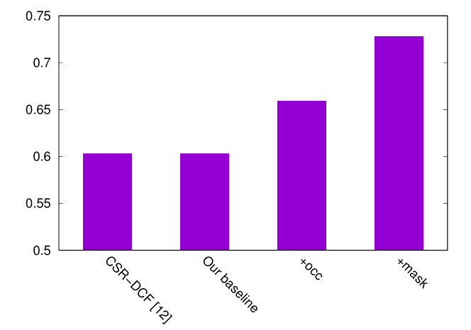
Figure 4: Ablation study of the components of our methods.(Numbers represent the average accuracy over 11 categories in the dataset)

We conducted a set of ablation studies to support our design choices. Moreover, we also evaluated our algorithm on the original Princeton Dataset which has considerable amount of registration and synchronization errors. We report the accuracy for the following variants:

• CSR-DCF State-of-the-art RGB tracker by Lukezic et al.  [15]

• DM-DCF– Our method with the all proposed components switched off.

• +occ Depth based occlusion handling switched on.

• +mask Depth based masking added i.e. full DM-DCF.

As it can be seen in Fig. 4, adding depth based masking and occlusion handling improve the results almost $\%15$.

IV-E Summary

An important finding for the future work is that in general, different algorithms favor certain categories and motion types. As compared the results of all methods in Table I, most of the methods favor rigid motion over non-rigid motion (rigid vs. animal categories). This can be explained by the fact that the parameters are kept constant for all 95 test sequences and the adopted parameters favors rigid object tracking. Shape changes and adaptation speeds are different for non-rigid objects such as animals.

Another similar problem can be seen in occlusion vs. no occlusion. Again, improvement in the occlusion sequences means slight degradation in tracker performance in no occlusion cases. These observations suggest us to adopt adaptive parameters in our future work so that the tracker would adjust its parameters on the fly according to the target object.

V Conclusion

In this paper, we proposed a Depth Masked Discriminative Correlation Filter (DM-DCF) RGBD tracker that uses the depth cue to detect occlusions (enable switching from the tracking to the detection mode) and to construct a spatial mask that improves DCF tracking. To this end, we are the first to use depth based segmentation masks inherently in DCF formulation extracting target regions for filter updates. Comparison and ablation studies on the publicly available Princeton RGBD Benchmark dataset verified that our trackers is on pair with the state-of-the-art while providing clearly better frame rate as compared to the top performers.

References

- [1] N. An, X.-G. Zhao, and Z.-G. Hou. Online rgb-d tracking via detection-learning-segmentation. In ICPR, 2016.
- [2] A. Bibi, T. Zhang, and B. Ghanem. 3d part-based sparse tracker with automatic synchronization and registration. In CVPR, 2016.
- [3] D. Bolme, J. Beveridge, B. Draper, and Y. Lui. Visual object tracking using adaptive correlation filters. In CVPR, 2010.
- [4] S. Boyd. Distributed optimization and statistical learning via the alternating direction method of multipliers. Foundations and Trends in Machine Learning, 3, 2010.
- [5] D. Comaniciu, V. Ramesh, and P. Meer. Kernel-based object tracking. IEEE Transactions on Pattern Analysis and Machine Intelligence, volume 25, pages 564–567, 2003.
- [6] N. Dalal and B. Triggs. Histograms of oriented gradients for human detection. In CVPR, 2005.
- [7] M. Danelljan, G. Bhat, F. Shahbaz Khan, and M. Felsberg. Eco: Efficient convolution operators for tracking. In CVPR, 2017.
- [8] M. Danelljan, A. Robinson, F. Shahbaz Khan, and M. Felsberg. Beyond Correlation Filters: Learning Continuous Convolution Operators for Visual Tracking. In ECCV, 2016.
- [9] H. Galoogahi, T. Sim, and S. Lucey. Correlation filters with limited boundaries. In CVPR, 2015.
- [10] S. Hannuna, M. Camplani, J. Hall, M. Mirmehdi, D. Damen, T. Burghardt, A. Paiement, and L. Tao. Ds-kcf: a real-time tracker for rgb-d data. In Journal of Real-Time Image Processing, 2016.
- [11] J. Henriques, R. Caseiro, P. Martins, and J. Batista. High-Speed Tracking with Kernelized Correlation Filters. In IEEE Transactions on Pattern Analysis and Machine Intelligence, volume 37, pages 1–14, 2014.
- [12] C. Hester and D. Casasent. Multivariant technique for multiclass pattern recognition. In Applied Optics, volume 19, pages 1758–1761, 1980.
- [13] Z. Kalal, K. Mikolajczyk, and J. Matas. Tracking-Learning-Detection. In IEEE Transactions on Pattern Analysis and Machine Intelligence, volume 34, pages 1409–1422, 2011.
- [14] M. Kristan, J. Matas, G. Nebehay, F. Porikli, and L. Cehovin. A Novel Performance Evaluation Methodology for Single-Target Trackers. In IEEE Transactions on Pattern Analysis and Machine Intelligence, volume 38, pages 2137–2155, 2016.
- [15] A. Lukezic, T. Vojir, L. Cehovin, J. Matas, and M. Kristan. Discriminative correlation filter with channel and spatial reliability. In CVPR, 2017.
- [16] K. Meshgi, S. I. Maeda, S. Oba, H. Skibbe, Y. Z. Li, and S. Ishii. An occlusion-aware particle filter tracker to handle complex and persistent occlusions. Computer Vision and Image Understanding, 150:81–94, 2016.
- [17] H. Nam and B. Han. Learning Multi-Domain Convolutional Neural Networks for Visual Tracking. In CVPR, 2016.
- [18] N. Otsu. A threshold selection method from gray-level histograms. IEEE Trans. Sys., Man., Cyber., 1979.
- [19] D. A. Ross, J. Lim, R.-S. Lin, and M.-H. Yang. Incremental visual tracking. International Journal of Computer Vision (IJCV), 77:125–141, 2008.
- [20] A. W. M. Smeulders, D. M. Chu, R. Cucchiara, S. Calderara, A. Dehghan, and M. Shah. Visual tracking: An experimental survey. volume 36, pages 1442–1468, 2014.
- [21] S. Song and J. Xiao. Tracking revisited using rgbd camera: Unified benchmark and baselines. In ICCV, 2013.
- [22] J. van de Weijer, C. Schmid, J. Verbeek, and D. Larlus. Learning color names for real-world applications. In IEEE Transactions on Pattern Analysis and Machine Intelligence, volume 18, pages 1512–1523, 2009.
- [23] T. Zhang, S. Liu, C. Xu, S. Yan, B. Ghanem, N. Ahuja, and M.-H. Yang. Structural sparse tracking. In CVPR, 2015.
- [24] Matej Kristan, Ales Leonardis, Jiri Matas, Michael Felsberg, Roman Pflugfelder, Luka Cehovin Zajc, Tomas Vojir, Gustav Hager, Alan Lukezic, Abdelrahman Eldesokey and Gustavo Fernandez The Visual Object Tracking VOT2017 Challenge Results. In ICCV, 2017.