Solving k-center Clustering (with Outliers) in MapReduce and Streaming, almost as Accurately as Sequentially.

Abstract.

Center-based clustering is a fundamental primitive for data analysis and becomes very challenging for large datasets. In this paper, we focus on the popular $k$-center variant which, given a set $S$ of points from some metric space and a parameter $k<|S|$, requires to identify a subset of $k$ centers in $S$ minimizing the maximum distance of any point of $S$ from its closest center. A more general formulation, introduced to deal with noisy datasets, features a further parameter $z$ and allows up to $z$ points of $S$ (outliers) to be disregarded when computing the maximum distance from the centers. We present coreset-based 2-round MapReduce algorithms for the above two formulations of the problem, and a 1-pass Streaming algorithm for the case with outliers. For any fixed $\varepsilon>0$, the algorithms yield solutions whose approximation ratios are a mere additive term $\varepsilon$ away from those achievable by the best known polynomial-time sequential algorithms, a result that substantially improves upon the state of the art. Our algorithms are rather simple and adapt to the intrinsic complexity of the dataset, captured by the doubling dimension $D$ of the metric space. Specifically, our analysis shows that the algorithms become very space-efficient for the important case of small (constant) $D$. These theoretical results are complemented with a set of experiments on real-world and synthetic datasets of up to over a billion points, which show that our algorithms yield better quality solutions over the state of the art while featuring excellent scalability, and that they also lend themselves to sequential implementations much faster than existing ones.

1. Introduction

Center-based clustering is a fundamental unsupervised learning primitive for data management, with applications in a variety of domains such as database search, bioinformatics, pattern recognition, networking, facility location, and many more (HennigMMR15, ). Its general goal is to partition a set of data items into groups according to a notion of similarity, captured by closeness to suitably chosen group representatives, called centers. There is an ample and well-established literature on sequential strategies for different instantiations of center-based clustering (AwasthiB15, ). However, the explosive growth of data that needs to be processed often rules out the use of these strategies which are efficient on small-sized datasets, but impractical on large ones. Therefore, it is of paramount importance to devise efficient clustering strategies tailored to the typical computational frameworks for big data processing, such as MapReduce and Streaming (LeskovecRU14, ).

In this paper, we focus on the $k$-center problem, formally defined as follows. Given a set $S$ of points in a metric space and a positive integer $k<|S|$, find a subset $T\subseteq S$ of $k$ points, called centers, so that the maximum distance between any point of $S$ to its closest center in $T$ is minimized. (Note that the association of each point to the closest center naturally defines a clustering of $S$.) Along with $k$-median and $k$-means, which require to minimize, respectively, the sum of all distances and all square distances to the closest centers, $k$-center is a very popular instantiation of center-based clustering which has recently proved a pivotal primitive for data and graph analytics (IndykMMM14, ; AghamolaeiFZ15, ; CeccarelloPPU15, ; CeccarelloPPU16, ; CeccarelloPPU17, ; CeccarelloFPPV17, ), and whose efficient solution in the realm of big data has attracted a lot of attention in the literature (Charikar2001, ; McCutchen2008, ; EneIM11, ; MalkomesKCWM15, ).

The $k$-center problem is NP-hard (Gonzalez85, ), therefore one has to settle for approximate solutions. Also, since its objective function involves a maximum, the solution is at risk of being severely influenced by a few “distant” points, called outliers. In fact, the presence of outliers is inherent in many datasets, since these points are often artifacts of data collection, or represent noisy measurements, or simply erroneous information. To cope with this problem, $k$-center admits a formulation that takes into account outliers (Charikar2001, ): when computing the objective function, up to $z$ points are allowed to be discarded, where $z$ is a user-defined input parameter.

A natural approach to compute approximate solutions to large instances of combinatorial optimization problems entails efficiently extracting a much smaller subset of the input, dubbed coreset, which contains a good approximation to the global optimum, and then applying a standard sequential approximation algorithm to such a coreset. The benefits of this approach are evident when the coreset construction is substantially more efficient than running the (possibly very expensive) sequential approximation algorithm directly on the whole input, so that significant performance improvements are attained by confining the execution of such algorithm on a small subset of the data. Using coresets much smaller than the input, the authors of (MalkomesKCWM15, ) present MapReduce algorithms for the $k$-center problem with and without outliers, whose (constant) approximation factors are, however, substantially larger than their best sequential counterparts. In this work, we further leverage the coreset approach and unveil interesting tradeoffs between the coreset size and the approximation quality, showing that better approximation is achievable through larger coresets. The obtainable tradeoffs are regulated by the doubling dimension of the underlying metric space and allow us to obtain improved MapReduce and Streaming algorithms for the two formulations of the $k$-center problem, whose approximation ratios can be made arbitrarily close to the one featured by the best sequential algorithms. Also, as a by-product, we obtain a sequential algorithm for the case with outliers which is considerably faster than existing ones.

1.1. Related work

Back in the 80’s, Gonzalez (Gonzalez85, ) developed a very popular 2-approximation sequential algorithm for the $k$-center problem running in $O\left(k|S|\right)$ time, which is referred to as gmm in the recent literature. In the same paper, the author showed that it is impossible to achieve an approximation factor $2-\varepsilon$, for fixed $\varepsilon>0$, in general metric spaces, unless $P=NP$. To deal with noise in the dataset, Charikar et al. (Charikar2001, ) introduced the $k$-center problem with $z$ outliers, where the clustering is allowed to ignore $z$ points of the input. For this problem, they gave a 3-approximation algorithm which runs in $O\left(k|S|^{2}\log|S|\right)$ time. Furthermore, they proved that, for this problem, it is impossible to achieve an approximation factor $3-\varepsilon$, for fixed $\varepsilon>0$, in general metric spaces, unless $P=NP$.

With the advent of big data, a lot of attention has been devoted to the MapReduce model of computation, where a set of processors with limited-size local memories process data in a sequence of parallel rounds (DeanG08, ; PietracaprinaPRSU12, ; LeskovecRU14, ). The $k$-center problem under this model was first studied by Ene et al. (EneIM11, ), who provided a 10-approximation randomized algorithm. This result was subsequently improved in (MalkomesKCWM15, ) with a deterministic 4-approximation algorithm requiring an $O\left(\sqrt{|S|k}\right)$-size local memory. As for the $k$-center problem with $z$ outliers, a deterministic $13$-approximation MapReduce algorithm was presented in (MalkomesKCWM15, ), requiring an $O\left(\sqrt{|S|(k+z)}\right)$-size local memory. We remark that randomized multi-round MapReduce algorithms for the two formulations of the $k$-center problem, with approximation ratios $2$ and 4 respectively, have been claimed but not described in the short communication (ImM15, ). While, theoretically, the MapReduce algorithms proposed in our work seem competitive with respect to both round complexity and space requirements with the algorithms announced in (ImM15, ), any comparison is clearly subject to the availability of more details.

As mentioned before, the algorithms in (MalkomesKCWM15, ) are based on the use of (composable) coresets, a very useful tool in the MapReduce setting (Agarwal2004, ; IndykMMM14, ). For a given objective function, a coreset is a small subset extracted from the input which embodies a solution whose cost is close to the cost of the optimal solution on the whole set. The additional property of composability requires that, if coresets are extracted from distinct subsets of a given partition of the input, their union embodies a close-to-optimal solution of the whole input. Composable coresets enable the development of parallel algorithms, where each processor computes the coreset relative to one subset of the partition, and the computation of the final solution is then performed by one processor that receives the union of the coresets. Composable coresets have been used for a number of problems, including diversity maximization (IndykMMM14, ; AghamolaeiFZ15, ; CeccarelloPPU17, ; CeccarelloPP18, ), submodular maximization (Mirrokni2015, ), graph matching and vertex cover (Assadi2017, ). In (BadoiuHI02, ) the authors provide a coreset-based $(1+\varepsilon)$-approximation sequential algorithm to the $k$-center problem for $d$-dimensional Euclidean spaces, whose time is exponential in $k$ and $(1/\varepsilon)^{2}$ and linear in $d$ and $|S|$. However, the coreset construction is rather involved, not easily parallelizable and the resulting algorithm seems to be mainly of theoretical interest.

Another option when dealing with large amounts of data is to process the data in a streaming fashion. In the Streaming model, algorithms use a single processor with limited working memory and are allowed only a few sequential passes over the input (ideally just one) (HenzingerRR98, ; LeskovecRU14, ). Originally developed for the external memory setting, this model also captures the scenario in which data is generated on the fly and must be analyzed in real-time, for instance in a streamed DMBS or in a social media platform (e.g., Twitter trends detection). Under this model, Charikar et al. (CharikarCFM04, ) developed a 1-pass algorithm for the $k$-center problem which requires $\Theta\left(k\right)$ working memory and computes an 8-approximation, deterministically, or a 5.43-approximation, probabilistically. Later, the result was improved in (McCutchen2008, ) attaining a $(2+\varepsilon)$ approximation, deterministically, needing a working memory of size $\Theta\left(k\varepsilon^{-1}\log(\varepsilon^{-1})\right)$. In the same paper, the authors give a deterministic $(4+\varepsilon)$-approximation Streaming algorithm for the formulation with $z$ outliers, which requires $O\left(kz\varepsilon^{-1}\right)$ working memory.

1.2. Our contribution

The coreset-based MapReduce algorithms of (MalkomesKCWM15, ) for $k$-center, with and without outliers, use the gmm sequential approximation algorithm for $k$-center in a “bootstrapping” fashion: namely, in a first phase, a set of $k$ centers ($k+z$ centers in the case with $z$ outliers) is determined in each subset of an arbitrary partition of the input dataset, and then the final solution is computed on the coreset provided by the union of these centers, using a sequential approximation algorithm for the specific problem formulation. Our work is motivated by the following natural question: what if we select more centers from each subset of the partition in the first phase? Intuitively, we should get a better solution than if we just selected $k$ (resp., $k+z$) centers. In fact, selecting more and more centers from each subset should yield a solution progressively closer to the one returned by the best sequential algorithm on the whole input, at the expense of larger space requirements.

This paper provides a thorough characterization of the space-accuracy tradeoffs achievable by exploiting the aforementioned idea for both formulations of the $k$-center problem (with and without outliers). We present improved MapReduce and Streaming algorithms which leverage a judicious selection of larger (composable) coresets to boost the quality of the solution embodied in the (union of the) coresets. We analyze the memory requirements of our algorithms in terms of the desired approximation quality, captured by a precision parameter $\varepsilon$, and of the doubling dimension $D$ of the underlying metric space, a parameter that generalizes the dimensionality of Euclidean spaces to arbitrary metric spaces and is thus related to the difficulty of spotting good clusterings. We remark that this kind of parametrized analysis is particularly relevant in the realm of big data, where distortions introduced to account for worst-case scenarios may be too extreme to provide meaningful insights on actual algorithm’s performance, and it has been employed in a variety of contexts including diversity maximization, clustering, nearest neighbour search, routing, machine learning, and graph analytics (see (CeccarelloPPU17, ) and references therein).

Our specific results are the following:

• A deterministic 2-round, $(2+\varepsilon)$-approximation MapReduce algorithm for the $k$-center problem, which requires $O\left(\sqrt{|S|k}(4/\varepsilon)^{D}\right)$ local memory.

• A deterministic 2-round, $(3+\varepsilon)$-approximation MapReduce algorithm for the $k$-center problem with $z$ outliers, which requires $O\left(\sqrt{|S|(k+z)}(24/\varepsilon)^{D}\right)$ local memory.

• A randomized 2-round, $(3+\varepsilon)$-approximation MapReduce algorithm for the $k$-center problem with $z$ outliers, which reduces the local memory requirements to $O\left(\left(\sqrt{|S|(k+\log|S|)}+z\right)(24/\varepsilon)^{D}\right)$.

• A deterministic 1-pass, $(3+\varepsilon)$-approximation Streaming algorithm for the $k$-center problem with $z$ outliers, which requires $O\left((k+z)(96/\varepsilon)^{D}\right)$ working memory.

Using our coreset constructions we can also attain a $(2+\varepsilon)$-approximation Streaming algorithm for $k$-center without outliers, which however would not improve on the state-of-the-art algorithm (McCutchen2008, ). Nonetheless, for the sake of completeness, we will compare these two algorithms experimentally in Section 5.

Observe that for both formulations of the problem, our algorithms feature approximation guarantees which are a mere additive term $\varepsilon$ larger than the best achievable sequential guarantee, and yield substantial quality improvements over the state-of-the-art (MalkomesKCWM15, ; McCutchen2008, ). Moreover, the randomized MapReduce algorithm for the formulation with outliers features smaller coresets, thus attaining a reduction in the local memory requirements which becomes substantial in plausible scenarios where the number of outliers $z$ (e.g., due to noise) is considerably larger than the target number $k$ of clusters, although much smaller than the input size.

While our algorithms are applicable to general metric spaces, on spaces of constant doubling dimension $D$ and for constant $\varepsilon$, their local space/working memory requirements are polynomially sublinear in the dataset size, in the MapReduce setting, and independent of the dataset size, in the Streaming setting. Moreover, a very desirable feature of our MapReduce algorithms is that they are oblivious to $D$, in the sense that the value $D$ (which may be not known in advance and hard to evaluate) is not used explicitly in the algorithms but only in their analysis. In contrast, the 1-pass Streaming algorithm makes explicit use of $D$, although we will show that it can be made oblivious to $D$ at the expense of one extra pass on the input stream.

As a further important result, the MapReduce algorithm for the case with outliers admits a direct sequential implementation which substantially improves the time performance of the state-of-the-art algorithm by (Charikar2001, ) while essentially preserving the approximation quality.

We also provide experimental evidence of the competitiveness of our algorithms on real-world and synthetic datasets of up to over a billion points, comparing with baselines set by the algorithms in (MalkomesKCWM15, ) for MapReduce, and (McCutchen2008, ) for Streaming. In the MapReduce setting, the experiments show that tighter approximations over the algorithms in (MalkomesKCWM15, ) are indeed achievable with larger coresets. In fact, while our theoretical bounds on the space requirements embody large constant factors, the improvements in the approximation quality are already noticeable with a modest increase of the coreset size. In the Streaming setting, for $k$-center without outliers we show that the $(2+\varepsilon)$-approximation algorithm based on our techniques is comparable to (McCutchen2008, ), whereas for $k$-center with outliers we obtain solutions of better quality using significantly less memory and time. The experiments also show that the Streaming algorithms feature high-throughput, and that the MapReduce algorithms exhibit high scalability. Finally, we show that, indeed, implementing our coreset strategy sequentially yields a substantial running time improvement with respect to the state-of-the art algorithm (Charikar2001, ), while preserving the approximation quality.
Organization of the paper The rest of the paper is organized as follows. Section 2 contains a number of preliminary concepts. Section 3 and Section 4 present, respectively, our MapReduce and Streaming algorithms. The experimental results are reported in Section 5. Finally, Section 6 offers some concluding remarks.

2. Preliminaries

Consider a metric space $\mathcal{S}$ with distance function $d(\cdot,\cdot)$. For a point $u\in\mathcal{S}$, the ball of radius $r$ centered at $u$ is the set of points at distance at most $r$ from $u$. The doubling dimension of $\mathcal{S}$ is the smallest $D$ such that for any radius $r$ and point $u\in\mathcal{S}$, all points in the ball of radius $r$ centered at $u$ are included in the union of at most $2^{D}$ balls of radius $r/2$ centered at suitable points. It immediately follows that, for any $0<\varepsilon\leq 1$, a ball of radius $r$ can be covered by at most $(1/\varepsilon)^{D}$ balls of radius $\varepsilon r$. Notable examples of metric spaces with bounded doubling dimension are Euclidean spaces and spaces induced by shortest-path distances in mildly-expanding topologies. Also, the notion of doubling dimension can be defined for an individual dataset and it may turn out much lower than the one of the underlying metric space (e.g., a set of collinear points in $\Re^{2}$). In fact, the space-accuracy tradeoffs of our algorithms only depend on the doubling dimension of the input dataset.

Define the distance between a point $s\in\mathcal{S}$ and a set $X\subseteq\mathcal{S}$ as $d(s,X)=\min_{x\in X}d(s,x)$. Consider now a dataset $S\subseteq\mathcal{S}$ and a subset $T\subseteq S$. We define the radius of $S$ with respect to $T$ as

$$r_{T}(S)=\max_{s\in S}d(s,T).$$

The $k$-center problem requires to find a subset $T\subseteq S$ of size $k$ such that $r_{T}(S)$ is minimized. We define $r_{k}^{*}(S)$ as the radius achieved by the optimal solution to the problem. Note that $T$ induces immediately a partition of $S$ into $k$ clusters by assigning each point to its closest center, and we say that $r_{T}(S)$ is the radius of such a clustering.

In Section 1.1 we mentioned the gmm algorithm (Gonzalez85, ), which provides a sequential 2-approximation to the $k$-center problem. Here we briefly review how gmm works. Given a set $S$, gmm builds a set of centers $T$ incrementally in $k$ iterations. An arbitrary point of $S$ is selected as the first center and is added to $T$. Then, the algorithm iteratively selects the next center as the point with maximum distance from $T$, and adds it to $T$, until $T$ contains $k$ centers. Note that, rather than setting $k$ a priori, gmm can be used to grow the set $T$ until a target radius is achieved. In fact, the radius of $S$ with respect to the set of centers $T$ incrementally built by gmm is a non-increasing function of the iteration number. In this paper, we will make use of the following property of gmm which bounds its accuracy when run on a subset of the data.

Lemma 0.

Let $X\subseteq S$. For a given $k$, let $T_{X}$ be the output of gmm when run on $X$. We have $r_{T_{X}}(X)\leq 2\cdot r_{k}^{*}(S)$.

Proof.

We prove this lemma by rephrasing the proof by Gonzalez (Gonzalez85, ) in terms of subsets. We need to prove that, $\forall x\in X$, $d(x,T_{X})\leq 2\cdot r_{k}^{*}(S)$. Assume by contradiction that this is not the case. Then, for some $y\in X$ it holds that $d(y,T_{X})>2\cdot r_{k}^{*}(S)$. By the greedy choice of gmm, we have that for any pair $t_{1},t_{2}\in T_{X}$, $d(t_{1},t_{2})\geq d(y,T_{X})$, otherwise $y$ would have been included in $T_{X}$. So we have that $d(t_{1},t_{2})>2\cdot r_{k}^{*}(S)$. Therefore, the set $\{y\}\cup T_{X}$ consists of $k+1$ points at distance $>2\cdot r_{k}^{*}(S)$ from each other. Consider now the optimal solution to $k$-center on the set $S$. Since $(\{y\}\cup T_{X})\subseteq S$, two of the $k+1$ points of $\{y\}\cup T_{X}$, say $x_{1}$ and $x_{2}$, must be closest to the same optimal center $o^{*}$. By the triangle inequality we have $2\cdot r_{k}^{*}(S)<d(x_{1},x_{2})\leq d(x_{1},o^{*})+d(o^{*},x_{2})\leq 2\cdot r_{k}^{*}(S)$, a contradiction. ∎

For a given set $S\subseteq\mathcal{S}$, the $k$-center problem with $z$ outliers requires to identify a set $T$ of $k$ centers which minimizes

$$r_{T,Z_{T}}(S)=\max_{s\in S\setminus Z_{T}}d(s,T),$$

where $Z_{T}$ is the set of $z$ points in $S$ with largest distance from $T$ (ties broken arbitrarily). In other words, the problem allows to discard up the $z$ farthest points when computing the radius of the set of centers, hence of its associated clustering. For given $S$, $k$, and $z$, we denote the radius of the optimal solution of this problem by $r_{k,z}^{*}(S)$. It is straightforward to argue that the optimal solution of the problem without outliers with $k+z$ centers has a smaller radius than the optimal solution of the problem with $k$ centers and $z$ outliers, that is

(1) $$r_{k+z}^{*}(S)\leq r_{k,z}^{*}(S).$$

2.1. Computational frameworks

A MapReduce algorithm (DeanG08, ; PietracaprinaPRSU12, ; LeskovecRU14, ) executes in a sequence of parallel rounds. In a round, a multiset $X$ of key-value pairs is first transformed into a new multiset $X^{\prime}$ of key-value pairs by applying a given map function (simply called mapper) to each individual pair, and then into a final multiset $Y$ of pairs by applying a given reduce function (simply called reducer) independently to each subset of pairs of $X^{\prime}$ having the same key. The model features two parameters, $M_{L}$, the local memory available to each mapper/reducer, and $M_{A}$, the aggregate memory across all mappers/reducers. In our algorithms, mappers are straightforward constant-space transformations, thus the memory requirements will be related to the reducers. We remark that the MapReduce algorithms presented in this paper also afford an immediate implementation and similar analysis in the Massively Parallel Computation (MPC) model (BeameKS13, ), which is popular in the database community.

In the Streaming framework (HenzingerRR98, ; LeskovecRU14, ) the computation is performed by a single processor with a small working memory, and the input is provided as a continuous stream of items which is usually too large to fit in the working memory. Multiple passes on the input stream may be allowed. Key performance indicators are the size of the working memory and the number of passes.

The holy grail of big data algorithmics is the development of MapReduce (resp., Streaming) algorithms which work in as few rounds (resp., passes) as possible and require substantially sublinear local memory (resp., working memory) and linear aggregate memory.

3. MapReduce algorithms

The following subsections present our MapReduce algorithms for the $k$-center problem (Subsection 3.1) and the $k$-center problem with $z$ outliers (Subsection 3.2). The algorithms are based on the use of composable coresets, which were reviewed in the introduction, and can be viewed as improved variants of those by (MalkomesKCWM15, ). The main novelty of our algorithms is their leveraging a judiciously increased coreset size to attain approximation qualities that are arbitrarily close to the ones featured by the best known sequential algorithms. Also, in the analysis, we relate the required coreset size to the doubling dimension of the underlying metric space (whose explicit knowledge, however, is not required by the algorithms) showing that coreset sizes stay small for spaces of bounded doubling dimension.

3.1. MapReduce algorithm for $k$-center

Consider an instance $S$ of the $k$-center problem and fix a precision parameter $\varepsilon\in(0,1]$, which will be used to regulate the approximation ratio. The MapReduce algorithm works in two rounds. In the first round, $S$ is partitioned into $\ell$ subsets $S_{i}$ of equal size, for $1\leq i\leq\ell$. In parallel, on each $S_{i}$ we run gmm incrementally and call $T_{i}^{j}$ the set of $j$ centers selected in the first $j$ iterations of the algorithm. Let $r_{T_{i}^{k}}(S_{i})$ denote the radius of the set $S_{i}$ with respect to the first $k$ centers. We continue to run gmm until the first iteration $\tau_{i}\geq k$ such that $r_{T_{i}^{\tau_{i}}}(S_{i})\leq\varepsilon/2\cdot r_{T_{i}^{k}}(S_{i})$, and define the coreset $T_{i}=T_{i}^{\tau_{i}}$. In the second round, the union of the coresets $T=\bigcup_{i=1}^{\ell}T_{i}$ is gathered into a single reducer and gmm is run on $T$ to compute the final set of $k$ centers. In what follows, we show that these centers are a good solution to the $k$-center problem on $S$.

The analysis relies on the following two lemmas which state that each input point has a close-by representative in $T$ and that $T$ has small size. We define a proxy function $p:S\to T$ that maps each $s\in S_{i}$ into the closest point in $T_{i}$, for every $1\leq i\leq\ell$. The following lemma is an easy consequence of Lemma 1.

Lemma 0.

For each $s\in S$, $d(s,p(s))\leq\varepsilon\cdot r_{k}^{*}(S)$.

Proof.

Fix $i\in[1,\ell]$, and consider $S_{i}\subseteq S$, and the set $T_{i}^{k}$ computed by the first $k$ iterations of gmm. Since $S_{i}$ is a subset of $S$, by Lemma 1 we have that $r_{T_{i}^{k}}(S_{i})\leq 2\cdot r_{k}^{*}(S)$. By construction, we have that $r_{T_{i}}(S_{i})\leq\varepsilon/2\cdot r_{T_{i}^{k}}(S_{i})$, hence $r_{T_{i}}(S_{i})\leq\varepsilon r_{k}^{*}(S)$. Consider now the proxy function $p$. For every $1\leq i\leq\ell$ and $s\in S_{i}$, it holds that $d(s,p(s))\leq r_{T_{i}}(S_{i})\leq\varepsilon r_{k}^{*}(S)$. ∎

We can conveniently bound the size of $T$, the union of the coresets, as a function of the doubling dimension of the underlying metric space.

Lemma 0.

If $S$ belongs to a metric space of doubling dimension $D$, then

$$|T|\leq\ell\cdot k\cdot\left(\frac{4}{\varepsilon}\right)^{D}.$$

Proof.

Fix an $i\in[1,\ell]$. We prove an upper bound on the number $\tau_{i}$ of iterations of gmm needed to obtain $r_{T_{i}^{\tau_{i}}}(S_{i})\leq(\varepsilon/2)r_{T_{i}^{k}}(S_{i})$, which in turn bounds the size of $T_{i}$. Consider the $k$-center clustering of $S_{i}$ induced by the $k$ centers in $T_{i}^{k}$, with radius $r_{T_{i}^{k}}(S_{i})$. By the doubling dimension property, we have that each of the $k$ clusters can be covered using at most $(4/\varepsilon)^{D}$ balls of radius $\leq(\varepsilon/4)\cdot r_{T_{i}^{k}}(S_{i})$, for a total of at most $h=k(4/\varepsilon)^{D}$ such balls. Consider now the execution of $h$ iterations of the gmm algorithm on $S_{i}$. Let $T_{i}^{h}$ be the set of returned centers and let $x\in S_{i}$ be the farthest point of $S_{i}$ from $T_{i}^{h}$. The center selection process of the gmm algorithm ensures that any two points in $T_{i}^{h}\cup\{x\}$ are at distance at least $r_{T_{i}^{h}}(S_{i})$ from one another. Thus, since two of these points must fall into one of the $h$ aforementioned balls of radius $\leq(\varepsilon/4)\cdot r_{T_{i}^{k}}(S_{i})$, this implies immediately (by the triangle inequality) that

$$r_{T_{i}^{h}}(S_{i})\leq 2(\varepsilon/4)\cdot r_{T_{i}^{k}}(S_{i})=(\varepsilon/2)\cdot r_{T_{i}^{k}}(S_{i}).$$

Hence, after $h$ iterations we are guaranteed that gmm finds a set $T_{i}^{h}$ which meets the stopping condition. Therefore, $|T_{i}|=\tau_{i}\leq h=k(4/\varepsilon)^{D}$, for every $i\in[1,\ell]$, and the lemma follows. ∎

We now state the main result of this subsection.

Theorem 3.

Let $0<\varepsilon\leq 1$. If the points of $S$ belong to a metric space of doubling dimension $D$, then the above 2-round MapReduce algorithm computes a $(2+\varepsilon)$-approximation for the $k$-center problem with local memory $M_{L}=O\left(|S|/\ell+\ell\cdot k\cdot(4/\varepsilon)^{D}\right)$ and linear aggregate memory.

Proof.

Let $X$ be the solution found by gmm on $T$. Since $T\subseteq S$, from Lemma 1 it follows that $r_{X}(T)\leq 2\cdot r_{k}^{*}(S)$. Consider an arbitrary point $s\in S$, along with its proxy $p(s)\in T$, as defined before. By Lemma 1 we know that $d(s,p(s))\leq\varepsilon\cdot r_{k}^{*}(S)$. Let $x\in X$ be the center closest to $p(s)$. It holds that $d(x,p(s))\leq 2\cdot r_{k}^{*}(S)$. By applying the triangle inequality, we have that $d(x,s)\leq d(x,p(s))+d(p(s),s)\leq 2\cdot r_{k}^{*}(S)+\varepsilon\cdot r_{k}^{*}(S)=(2+\varepsilon)r_{k}^{*}(S)$. The bound on $M_{L}$ follows since in the first round each processor needs to store $|S|/\ell$ points of the input and computes a coreset of size $O\left(k\cdot(4/\varepsilon)^{D}\right)$, as per Lemma 2, while in the second round, one processor needs enough memory to store $\ell$ such coresets. Finally, it is immediate to see that aggregate memory proportional to the input size suffices. ∎

By setting $\ell=\Theta\left(\sqrt{|S|/k}\right)$ in the above theorem we obtain:

Corollary 0.

Our 2-round MapReduce algorithm computes a $(2+\varepsilon)$-approximation for the $k$-center problem with local memory $M_{L}=O\left(\sqrt{|S|k}(4/\varepsilon)^{D}\right)$ and linear aggregate memory. For constant $\varepsilon$ and $D$, the local memory bound becomes $M_{L}=O\left(\sqrt{|S|k}\right)$.

3.2. MapReduce algorithm for $k$-center with $z$ outliers

Consider an instance $S$ of the $k$-center problem with $z$ outliers and fix a precision parameter $\hat{\varepsilon}\in(0,1]$ intended, as before, to regulate the approximation ratio. We propose the following 2-round MapReduce algorithm for the problem. In the first round, $S$ is partitioned into $\ell$ equally-sized subsets $S_{i}$, with $1\leq i\leq\ell$, and for each $S_{i}$, in parallel, gmm is run incrementally. Let $T_{i}^{j}$ be the set of the first $j$ selected centers. We continue to run gmm until the first iteration $\tau_{i}\geq k+z$ such that $r_{T_{i}^{\tau_{i}}}(S_{i})\leq\hat{\varepsilon}/2\cdot r_{T_{i}^{k+z}}(S_{i})$. Define the coreset $T_{i}=T_{i}^{\tau_{i}}$. As before, for each point $s\in S_{i}$ we define its proxy $p(s)$ to be the point of $T_{i}$ closest to $s$, but, furthermore, we attach to each $t\in T_{i}$ a weight $w_{t}\geq 1$, which is the number of points of $S_{i}$ with proxy $t$.

In the second round, the union of the weighted coresets $T=\cup_{i=1}^{\ell}T_{i}$ is gathered into a single reducer. Before describing the details of this second round, we need to introduce a sequential algorithm, dubbed OutliersCluster  (see pseudocode below), for solving a weighted variant of the $k$-center problem with outliers which is a modification of the one presented in (MalkomesKCWM15, ) (in turn, based on the unweighted algorithm of (Charikar2001, )).

$T^{\prime}$ $\leftarrow$ $T$

$X$ $\leftarrow$ $\emptyset$

while $((|X|<k)\;\mbox{\bf and}\;(T^{\prime}\neq\emptyset))$ do

       for ($t\in T$) do  $B_{t}$ $\leftarrow$ $\{v:v\in T^{\prime}\wedge d(v,t)\leq(1+2\hat{\varepsilon})\cdot r\}$

       $x$ $\leftarrow$ $\operatorname*{arg\,max}_{t\in T}\sum_{v\in B_{t}}w_{v}$

       $X$ $\leftarrow$ $X\cup\{x\}$

       $E_{x}$ $\leftarrow$ $\{v:v\in T^{\prime}\wedge d(v,x)\leq(3+4\hat{\varepsilon})\cdot r\}$

       $T^{\prime}$ $\leftarrow$ $T^{\prime}\setminus E_{x}$

      

return $X,T^{\prime}$

Algorithm 1 OutliersCluster$(T,k,r,\hat{\varepsilon})$

OutliersCluster $(T,k,r,\hat{\varepsilon})$ returns two subsets $X,T^{\prime}\subseteq T$ such that $X$ is a set of (at most) $k$ centers, and $T^{\prime}$ is a set of points referred to as uncovered points. The algorithm starts with $T^{\prime}=T$ and builds $X$ incrementally in $|X|\leq k$ iterations as follows. In each iteration, the next center $x$ is chosen as the point maximizing the aggregate weight of uncovered points in its ball of radius $(1+2\hat{\varepsilon})\cdot r$ (note that $x$ needs not be an uncovered point). Then, all uncovered points at distance at most $(3+4\hat{\varepsilon})\cdot r$ from $x$ are removed from $T^{\prime}$. The algorithm terminates when either $|X|=k$ or $T^{\prime}=\emptyset$. By construction, the final $T^{\prime}$ consists of all points at distance greater than $(3+4\hat{\varepsilon})\cdot r$ from $X$.

Let us return to the second round of our MapReduce algorithm. The reducer that gathered $T$ runs OutliersCluster$(T,k,r,\hat{\varepsilon})$ multiple times to estimate the minimum value $r_{\rm min}$ such that the aggregate weight of the points in the set $T^{\prime}$ returned by OutliersCluster$(T,k,r_{\rm min},\hat{\varepsilon})$ is at most $z$. More specifically, the computed estimate, say $\tilde{r}_{\rm min}$, is within a multiplicative tolerance $(1+\delta)$ from the true $r_{\rm min}$, with $\delta=\hat{\varepsilon}/(3+4\hat{\varepsilon})$, and it is obtained through a binary search over all possible $O\left(|T|^{2}\right)$ distances between points of $T$ combined with a geometric search with step $(1+\delta)$. To avoid storing all $O\left(|T|^{2}\right)$ distances, the value of $r$ at each iteration of the binary search can be determined in space linear in $T$ by the median-finding Streaming algorithm in (MunroP80, ). The output of the MapReduce algorithm is the set of centers computed by OutliersCluster$(T,k,\tilde{r}_{\rm min},\hat{\varepsilon})$.

We now analyze our 2-round MapReduce algorithm. The following lemma bounds the distance between a point and its proxy.

Lemma 0.

For each $s\in S$, $d(s,p(s))\leq\hat{\varepsilon}\cdot r_{k,z}^{*}(S)$.

Proof.

Consider any subset $S_{i}$ of the partition $S_{1},\dots,S_{\ell}$ of $S$. By construction, we have that for each $s\in S_{i}$, $d(s,p(s))\leq(\hat{\varepsilon}/2)\cdot r_{T_{i}^{k+z}}(S_{i})$. Since $S_{i}$ is a subset of $S$, Lemma 1 ensures that $r_{T_{i}^{k+z}}(S_{i})\leq 2r^{*}_{k+z}(S)$. Hence, $d(s,p(s))\leq\hat{\varepsilon}r^{*}_{k+z}(S)$. Since $r^{*}_{k+z}(S)\leq r_{k,z}^{*}(S)$, as observed before in Eq. 1, we have $d(x,p(x))\leq\hat{\varepsilon}\cdot r_{k,z}^{*}(S)$. ∎

Next, we characterize the quality of the solution returned by OutliersCluster when run on $T$, the union of the weighted coresets, and with a radius $r\geq r_{k,z}^{*}(S)$.

Lemma 0.

For $r\geq r_{k,z}^{*}(S)$, let $X,T^{\prime}\subseteq T$ be the sets returned by OutliersCluster $(T,k,r,\hat{\varepsilon})$, and define $S_{T^{\prime}}=\{s\in S:p(s)\in T^{\prime}\}$. Then,

$$d(t,X)\leq(3+4\hat{\varepsilon})\cdot r\quad\forall t\in T\setminus T^{\prime}$$

and $|S_{T^{\prime}}|\leq z$.

Proof.

The proof uses an argument akin to the one used for the analysis of the sequential algorithm by (Charikar2001, ) and later adapted by (MalkomesKCWM15, ) to the weighted coreset setting. The first claim follows immediately from the workings of the algorithm, since each point in $T-T^{\prime}$ belongs to some $E_{x}$, with $x\in X$. We are left to show that $|S_{T^{\prime}}|\leq z$. Suppose first that $|X|<k$. In this case, it must be $T^{\prime}=\emptyset$, hence $|S_{T^{\prime}}|=0$, and the proof follows. We now concentrate on the case $|X|=k$. Consider the $i$-th iteration of the while loop of OutliersCluster $(T,k,r,\hat{\varepsilon})$ and define $x_{i}$ as the center of $X$ selected in the iteration, and $T^{\prime}_{i}$ as the set $T^{\prime}$ of uncovered points at the beginning of the iteration. Recall that $x_{i}$ is the point of $T$ which maximizes the cumulative weight of the set $B_{x_{i}}$ of uncovered points in $T^{\prime}_{i}$ at distance at most $(1+2\hat{\varepsilon})\cdot r$ from $x_{i}$, and that the set $E_{x_{i}}$ of all uncovered points at distance at most $(3+4\hat{\varepsilon})\cdot r$ from $x_{i}$ is removed from $T^{\prime}_{i}$ at the end of the iteration. We now show that

(2) $$\sum_{i=1}^{k}\sum_{t\in E_{x_{i}}}w_{t}\geq|S|-z,$$

which will immediately imply that $|S_{T^{\prime}}|\leq z$. For this purpose, let $O$ be an optimal set of $k$ centers for the problem instance under consideration, and let $Z$ be the set of at most $z$ outliers at distance greater than $r_{k,z}^{*}(S)$ from $O$. For each $o\in O$, define $C_{o}\subseteq S\setminus Z$ as the set of nonoutlier points which are closer to $o$ than to any other center of $O$, with ties broken arbitrarily. To prove (2), it is sufficient to exhibit an ordering $o_{1},o_{2},\ldots,o_{k}$ of the centers in $O$ so that, for every $1\leq i\leq k$, it holds

$$\sum_{j=1}^{i}\sum_{t\in E_{x_{j}}}w_{t}\geq|C_{o_{1}}\cup\dots\cup C_{o_{i}}|.$$

The proof uses an inductive charging argument to assign each point in $\bigcup_{j=1}^{i}C_{o_{j}}$ to a point in $\bigcup_{j=1}^{i}E_{x_{j}}$, where each $t$ in the latter set will be in charge of at most $w_{t}$ points. We define two charging rules. A point can be either charged to its own proxy (Rule 1) or to another point of $T$ (Rule 2).

Fix some arbitrary $i$, with $1\leq i\leq k$, and assume, inductively, that the points in $C_{o_{1}}\cup\dots\cup C_{o_{i-1}}$ have been charged to points in $\bigcup_{j=1}^{i-1}E_{j}$ for some choice of distinct optimal centers $o_{1},o_{2},\ldots,o_{i-1}$. We have two cases.
Case 1. There exists an optimal center $o$ still unchosen such that there is a point $v\in C_{o}$ with $p(v)\in B_{x_{j}}$, for some $1\leq j\leq i$. We choose $o_{i}$ as one such center. Hence $d(x_{j},p(v))\leq(1+2\hat{\varepsilon})\cdot r$. By repeatedly applying the triangle inequality we have that for each $u\in C_{o_{i}}$

$$d(x_{j},p(u))\leq \;\;d(x_{j},p(v))+d(p(v),v)+d(v,o_{i})+d(o_{i},u)+$$

$$+d(u,p(u))\leq(3+4\hat{\varepsilon})\cdot r$$

hence, $p(u)\in E_{x_{j}}$. Therefore we can charge each point $u\in C_{o_{i}}$ to its proxy, by Rule 1.
Case 2. For each unchosen optimal center $o$ and each $v\in C_{o}$, $p(v)\not\in\bigcup_{j=1}^{i}B_{x_{j}}$. We choose $o_{i}$ to be the unchosen optimal center which maximizes the cardinality of $\{p(u):u\in C_{o_{i}}\}\cap T^{\prime}_{i}$. We distinguish between points $u\in C_{o_{i}}$ with $p(u)\notin T^{\prime}_{i}$, hence $p(u)\in\bigcup_{j=1}^{i-1}E_{x_{j}}$, and those with $p(u)\in T^{\prime}_{i}$. We charge each $u\in C_{o_{i}}$ with $p(u)\notin T^{\prime}_{i}$ to its own proxy by Rule 1. As for the other points, we now show that we can charge them to the points of $B_{x_{i}}$. To this purpose, we first observe that $B_{p(o_{i})}$ contains $\{p(u):u\in C_{o_{i}}\}\cap T^{\prime}_{i}$, since for each $u\in C_{o_{i}}$

$$d(p(o_{i}),p(u)) \leq d(p(o_{i}),o_{i})+d(o_{i},u)+d(u,p(u))$$

$$\leq(1+2\hat{\varepsilon})\cdot r_{k,z}^{*}(S)\leq(1+2\hat{\varepsilon})\cdot r.$$

Therefore the aggregate weight of $B_{p(o_{i})}$ is at least $\left|\left\{u\in C_{o_{i}}:p(u)\in T^{\prime}_{i}\right\}\right|$. Since Iteration $i$ selects $x_{i}$ as the center such that $B_{x_{i}}$ has maximum aggregate weight, we have that

$$\sum_{t\in B_{x_{i}}}w_{t}\geq\sum_{z\in B_{p(o_{i})}}w_{z}\geq\left|\left\{u\in C_{o_{i}}:p(u)\in T^{\prime}_{i}\right\}\right|,$$

hence, the points in $B_{x_{i}}$ have enough weight to be charged with each point $u\in C_{o_{i}}$ with $p(u)\in T^{\prime}_{i}$. Figure 1 illustrates the charging under Case 2.

Figure 1. Application of charging rules in case 2 of the proof. Round points are points of $S$, whereas star-shaped points are proxy points in $T$. Arrows represent charging.

Note that the points of $B_{x_{i}}$ did not receive any charging by Rule 1 in previous iterations, since they are uncovered at the beginning of Iteration $i$, and will not receive chargings by Rule 1 in subsequent iterations, since $B_{x_{i}}$ does not intersect the set $C_{o}$ of any optimal center $o$ yet to be chosen. Also, no further charging to points of $B_{x_{i}}$ by Rule 2 will happen in subsequent iterations, since Rule 2 will only target sets $B_{x_{h}}$ with $h>i$. These observations ensure that any point of $T$ receives charges through either Rule 1 or Rule 2, but not both, and never in excess of its weight, and the proof follows. ∎

The following lemma bounds the size of $T$, the union of the weighted coresets.

Lemma 0.

If $S$ belongs to a metric space of doubling dimension $D$, then

$$|T|\leq\ell\cdot(k+z)\cdot\left(\frac{4}{\hat{\varepsilon}}\right)^{D}$$

Proof.

The proof proceeds similarly to the one of Lemma 2, with the understanding that the definition of doubling dimension is applied to each of the $(k+z)$ clusters induced by the points of $T_{i}^{k+z}$ on $S_{i}$. ∎

Finally, we state the main result of this subsection.

Theorem 8.

Let $0<\varepsilon\leq 1$. If the points of $S$ belong to a metric space of doubling dimension $D$, then, when run with $\hat{\varepsilon}=\varepsilon/6$, the above 2-round MapReduce algorithm computes a $(3+\varepsilon)$-approximation for the $k$-center problem with $z$ outliers with local memory $M_{L}=O\left(|S|/\ell+\ell\cdot(k+z)\cdot(24/\varepsilon)^{D}\right)$ and linear aggregate memory.

Proof.

The result of Lemma 6 combined with the stipulated tolerance of the search performed in the second round of the algorithm implies that the radius discovered by the search is $\tilde{r}_{\rm min}\leq r_{k,z}^{*}(S)(1+\delta)$ with $\delta=\hat{\varepsilon}/(3+4\hat{\varepsilon})$. Also, by the triangle inequality, the distance between each non-outlier point in $S$ and its closest center will be at most $\hat{\varepsilon}r_{k,z}^{*}(S)+(3+4\hat{\varepsilon})r_{k,z}^{*}(S)(1+\delta)\leq(3+6\hat{\varepsilon})r_{k,z}^{*}(S)\leq(3+\varepsilon)r_{k,z}^{*}(S)$, which proves the approximation bound. The bound on $M_{L}$ follows since in the first round each reducer needs enough memory to store $|S|/\ell$ points of the input, while in the second round the reducer computing the final solution requires enough memory to store the union of the $\ell$ coresets, which, by Lemma 7, has size $O\left((k+z)(4/\hat{\varepsilon})^{D}\right)=O\left((k+z)(24/\varepsilon)^{D}\right)$ each. Also, globally, the reducers need only sufficient memory to store the input, hence $M_{A}=O\left(|S|\right)$. ∎

By setting $\ell=\Theta\left(\sqrt{|S|/(k+z)}\right)$ in the above theorem we obtain:

Corollary 0.

Our 2-round MapReduce algorithm computes a $(3+\varepsilon)$-approximation for the $k$-center problem with $z$ outliers, with local memory $M_{L}=O\left(\sqrt{|S|(k+z)}(24/\varepsilon)^{D})\right)$ and linear aggregate memory. For constant $\varepsilon$ and $D$, the local memory bound becomes $M_{L}=O\left(\sqrt{|S|(k+z)}\right)$.

Improved sequential algorithm. A simple analysis implies that, by setting $\ell=1$, our MapReduce strategy for the $k$-center problem with $z$ outliers yields an efficient sequential $(3+\varepsilon)$-approximation algorithm whose running time is $O\left(|S||T|+k|T|^{2}\log|T|\right)$, where $|T|=(k+z)(24/\varepsilon)^{D}$, is the coreset size. For a wide range of values of $k,z,\varepsilon$ and $D$ this yields a substantially improved performance over the $O\left(k|S|^{2}\log|S|\right)$-time state-of-the-art algorithm of (Charikar2001, ), at the expense of a negligibly worse approximation.

3.2.1. Higher space efficiency through randomization

The analysis of very noisy datasets might require setting the number $z$ of outliers much larger than $k$, while still $o(|S|)$. In this circumstance, the size of the union of the coresets $T$ is proportional to $\sqrt{|S|z}$, and may turn out too large for practical purposes, due to the large local memory requirements and to the running time of the cubic sequential approximation algorithm run on $T$ in the second round, which may become the real performance bottleneck of the entire algorithm. In this subsection, we show that this drawback can be significantly ameliorated by simply partitioning the pointset at random in the first round, at the only expense of probabilistic rather than deterministic guarantees on the resulting space and approximation guarantees. We say that an event related to a dataset $S$ occurs with high probability $p$ if $p\geq 1-1/|S|^{c}$, for some constant $c\geq 1$.

The randomized variant of the algorithm works as follows. In the first round, the input set $S$ is partitioned into $\ell$ subsets $S_{i}$, with $1\leq i\leq\ell$, by assigning each point to a random subset chosen uniformly and independently of the other points. Let $z^{\prime}=6((z/\ell)+\log_{2}|S|)$ and observe that, for large $z$ and $\ell$, we have that $z^{\prime}\ll z$. Then, in parallel on each partition $S_{i}$, gmm is run to yield a set $T_{i}^{\tau_{i}}$ of $\tau_{i}$ centers, where $\tau_{i}\geq k+z^{\prime}$ is the smallest value such that $r_{T_{i}^{\tau_{i}}}(S_{i})\leq(\hat{\varepsilon}/2)\cdot r_{T_{i}^{k+z^{\prime}}}(S_{i})$. Define the coreset $T_{i}=T_{i}^{\tau_{i}}$ and, again, for each point $s\in S_{i}$ define its proxy $p(s)$ to be the point of $T_{i}$ closest to $s$. The rest of the algorithm is exactly as before using these new $T_{i}$’s.

The analysis proceeds as follows. Consider an optimal solution of the $k$-center problem with $z$ outliers for $S$, and let $O=\{o_{1},o_{2},\ldots,o_{k}\}$ be the set of $k$ centers and $Z_{O}$ the set of $z$ outliers, that is the $z$ points of $S$ most distant from $O$. Recall that any point of $S\setminus Z_{O}$ is at distance at most $r_{k,z}^{*}(S)$ from $O$. The following lemma states that the outliers (set $Z_{O}$) are well distributed among the $S_{i}$’s.

Lemma 0.

With high probability, each $S_{i}$ contains no more than $z^{\prime}=6((z/\ell)+\log_{2}|S|)$ points of $Z_{O}$.

Proof.

The result follows by applying Chernoff bound (4.3) of (MitzemacherU17, ) and the union bound, which yield that the stated event occurs with probability at least $1-1/|S|^{5}$. ∎

The rest of the analysis mimics the one of the deterministic version.

Lemma 0.

The statements of both Lemmas 5 and 6 hold with high probability.

Proof.

We first prove that, with high probability, for each for each $s\in S$, $d(s,p(s))\leq\hat{\varepsilon}\cdot r_{k,z}^{*}(S)$ (same as Lemma 5). Consider $O$ and $Z_{O}$. We condition on the event that each $S_{i}$ contains at most $z^{\prime}$ points of $Z_{O}$, which, by Lemma 10, occurs with high probability. Focus on an arbitrary subset $S_{i}$. For $1\leq j\leq\ell$, let $C_{j}$ be the set of points of $S\setminus Z_{O}$ whose closest optimal center is $o_{j}$, and let $C_{j}(i)=C_{j}\cap S_{i}$. Consider the set $T_{i}^{k+z^{\prime}}$ of centers determined by the first $k+z^{\prime}$ iterations of the gmm algorithm and let $x\in S_{i}$ be the farthest point of $S_{i}$ from $T_{i}^{k+z^{\prime}}$. By arguing as in the proof of Lemma 2, it can be shown that any two points in $T_{i}^{k+z^{\prime}}\cup\{x\}$ are at distance at least $r_{T_{i}^{k+z^{\prime}}}(S_{i})$ from one another and since two of these points must belong to the same $C_{j}(i)$ for some $j$, by the triangle inequality we have that

$$r_{T_{i}^{k+z^{\prime}}}(S_{i})\leq 2r_{k,z}^{*}(S).$$

Recall that the gmm algorithm on $S_{i}$ is stopped at the first iteration $\tau_{i}$ such that $r_{T_{i}^{\tau_{i}}}(S_{i})\leq(\hat{\varepsilon}/2)\cdot r_{T_{i}^{k+z^{\prime}}}(S_{i})$, hence

$$r_{T_{i}^{\tau_{i}}}(S_{i})\leq(\hat{\varepsilon}/2)\cdot r_{T_{i}^{k+z^{\prime}}}(S_{i})\leq(\hat{\varepsilon}/2)\cdot 2r_{k,z}^{*}(S)=\hat{\varepsilon}\cdot r_{k,z}^{*}(S).$$

The desired bound on $d(s,p(s))$ immediately follows. Conditioning on this bound, the proof of Lemma 6 can be repeated identically, hence the stated property holds. ∎

By repeating the same argument used in Lemma 7, one can easily argue that, if $S$ belongs to a metric space of doubling dimension $D$, then the size of the weighted coreset $T$ is

$$|T|\leq\ell\cdot(k+z^{\prime})\cdot\left(\frac{4}{\hat{\varepsilon}}\right)^{D}.$$

This bound, together with the results of the preceding lemma, immediately implies the analogous of Theorem 8 stating that, with high probability, the randomized algorithm computes a $(3+\varepsilon)$-approximation for the $k$-center problem with $z$ outliers with local memory $M_{L}=O\left(|S|/\ell+\ell\cdot(k+z^{\prime})\cdot(24/\varepsilon)^{D}\right)$ and linear aggregate memory. Observe that $z$ is now replaced by (the much smaller) $z^{\prime}$ in the local memory bound.

By choosing $\ell=\Theta\left(\sqrt{|S|/(k+\log|S|)}\right)$ we obtain:

Corollary 0.

With high probability, our 2-round MapReduce algorithm computes a $(3+\varepsilon)$-approximation for the $k$-center problem with $z$ outliers, with local memory $M_{L}=O\left(\left(\sqrt{|S|(k+\log|S|)}+z\right)(24/\varepsilon)^{D}\right)$ and linear aggregate memory. For constant $\varepsilon$ and $D$, the local memory bound becomes $M_{L}=O\left(\sqrt{|S|(k+\log|S|)}+z\right)$

With respect to the deterministic version, for large values of $z$ a substantial improvement in the local memory requirements is achieved.
Remark. Thanks to the incremental nature of gmm, our coreset-based MapReduce algorithms for the $k$-center problem, both without and with outliers, need not know the doubling dimension $D$ of the underlying metric space in order to attain the claimed performance bounds. This is a very desirable property, since, in general, $D$ may not be known in advance. Moreover, if $D$ were known, a factor $\sqrt{(c/\varepsilon)^{D}}$ in local memory (where $c=4$ for $k$-center, and $c=24$ for $k$-center with $z$ outliers) could be saved by setting $\ell$ to be a factor $\Theta\left(\sqrt{(c/\varepsilon)^{D}}\right)$ smaller.

4. Streaming algorithm for $k$-center with $z$ outliers

As mentioned in the introduction, in the Streaming setting we will only consider the $k$-center problem with $z$ outliers. Consider an instance $S$ of the problem and fix a precision parameter $\hat{\varepsilon}\in(0,1]$. Suppose that the points of $S$ belong to a metric space of known doubling dimension $D$. Our Streaming algorithm also adopts a coreset-based approach. Specifically, in a pass over the stream of points of $S$ a suitable weighted coreset $T$ is selected and stored in the working memory. Then, at the end of the pass, the final set of centers is determined through multiple runs of OutliersCluster on $T$ as was done in the second round of the MapReduce algorithm described in Subsection 3.2. Below, we will focus on the coreset construction.

The algorithm computes a coreset $T$ of $\tau\geq k+z$ centers which represent a good approximate solution to the $\tau$-center problem on $S$ (without outliers). The value of $\tau$, which will be fixed later, depends on $\hat{\varepsilon}$ and $D$. The main difference with the MapReduce algorithm is the fact that we cannot exploit the incremental approach provided by gmm, since no efficient implementation of gmm in the Streaming setting is known. Hence, for the computation of $T$ we resort to a novel weighted variant of the doubling algorithm by Charikar et al. (CharikarCFM04, ) which is described below.

For a given stream of points $S$ and a target number of centers $\tau$, the algorithm maintains a weighted set $T$ of centers selected among the points of $S$ processed so far, and a lower bound $\phi$ on $r_{\tau}^{*}(S)$. $T$ is initialized with the first $\tau+1$ points of $S$, with each $t\in T$ assigned weight $w_{t}=1$, while $\phi$ is initialized to half the minimum distance between the points of $T$. For the sake of the analysis, we will define a proxy function $p:S\to T$ which, however, will not be explicitly stored by the algorithm. Initially, each point of $T$ is proxy for itself. The remaining points of $S$ are processed one at a time maintaining the following invariants:

1. $T$ contains at most $\tau$ centers.

2. $\forall t_{1},t_{2}\in T$ we have $d(t_{1},t_{2})>4\phi$

3. $\forall s\in S$ processed so far, $d(s,p(s))\leq 8\phi$.

4. $\forall t\in T$, $w_{t}=|\{s\in S\mbox{ processed so far}:\;p(s)=t\}|$.

5. $\phi\leq r_{\tau}^{*}(S)$.

The following two rules are applied to process each new point $s\in S$. The update rule checks if $d(s,T)\leq 8\phi$. If this is the case, the center $t\in T$ closest to $s$ is identified and $w_{t}$ is incremented by one, defining $p(s)=t$. If instead $d(s,T)>8\phi$, then $s$ is added as a new center to $T$, setting $w_{s}$ to 1 and defining $p(s)=s$. Note that in this latter case, the size of $T$ may exceed $\tau$, thus violating invariant (a). When this happens, the following merge rule is invoked repeatedly until invariant (a) is re-established. Each invocation of this rule first sets $\phi$ to $2\phi$, which, in turn, may lead to a violation of invariant (b). If this is the case, for each pair of points $u,v\in T$ violating invariant (b), we discard $u$ and set $w_{v}\leftarrow w_{v}+w_{u}$. Conceptually, this corresponds to the update of the proxy function which redefines $p(x)=v$, for each point $x$ for which $p(x)$ was equal to $u$.

Observe that, at the end of the initialization, invariants (a) and (b) do not hold, while invariants (c)$\div$(e) do hold. Thus, we prescribe that the merge rule and the reinforcement of invariant (b) are applied at the end of the initialization before any new point is processed. This will ensure that all invariants hold before the $(\tau+2)$nd point of $S$ is processed. The following lemma shows the above rules maintain all invariants.

Lemma 0.

After the initialization, at the end of the processing of each point $s\in S$, all invariants hold.

Proof.

As explained above, all invariants are enforced at the end of the initialization. Consider the processing of a new point $s$. It is straightforward to see that the combination of update and merge rules maintain invariants (a)-(d). We now show that invariant (e) is also maintained. After the update rule is applied, only invariant (a) can be violated. Suppose that this is the case, hence $|T|=\tau+1$. Each pair of centers in $T$ are at distance at least $4\phi$ from one another (invariant (b)). Let $\phi^{\prime}$ be the new value of $\phi$ resulting after the required applications of the merging rule. It is easy to see that until the penultimate application of the merge rule, $T$ still contains $\tau+1$ points. Therefore each pair of these points must be at distance at least $4(\phi^{\prime}/2)=2\phi^{\prime}$ from one another. This implies, that $\phi^{\prime}$ is still a lower bound to $r_{\tau}^{*}(S)$. ∎

As an immediate corollary of the previous lemma, we have that after all points of $S$ have been processed, $d(s,p(s))\leq 8\cdot r_{\tau}^{*}(S)$ for every $s\in S$. Moreover, it is immediate to see that the working memory required by the algorithm has size $\Theta\left(\tau\right)$. Fix now $\tau=(k+z)(16/\hat{\varepsilon})^{D}$ and let $T$ be the weighted coreset $T$ of size $\tau$ returned by the above algorithm. The following lemma is the counterpart of Lemma 5 in the Streaming setting.

Lemma 0.

For every $s\in S$, $d(s,p(s))\leq\hat{\varepsilon}\cdot r_{k,z}^{*}(S)$.

Proof.

Observe that $S$ can be covered using $k+z$ balls of radius $r_{k+z}^{*}(S)$. Since $S$ comes from a space of doubling dimension $D$, we know that $S$ can also be covered using $\tau=(k+z)(16/\hat{\varepsilon})^{D}$ balls (not necessarily centered at points in $S$) of radius $\leq\hat{\varepsilon}/16\cdot r_{k+z}^{*}(S)$. Picking an arbitrary center of $S$ from each such ball induces a $\tau$-clustering of $S$ with radius at most $\hat{\varepsilon}/8\cdot r_{k+z}^{*}(S)$. Hence,

$$r_{\tau}^{*}(S)\leq\hat{\varepsilon}/8\cdot r_{k+z}^{*}(S).$$

Since $r_{k+z}^{*}(S)\leq r_{k,z}^{*}(S)$, it follows that $r_{\tau}^{*}(S)\leq\hat{\varepsilon}/8\cdot r_{k,z}^{*}(S)$. By invariants (c) and (e) we have that for every $s\in S$

$$d(s,p(s))\leq 8\phi\leq 8\cdot r_{\tau}^{*}(S)\leq\hat{\varepsilon}\cdot r_{k,z}^{*}(S).\qed$$

∎

The following theorem states the main result of this section.

Theorem 3.

Let $0<\varepsilon\leq 1$. If the points of $S$ belong to a metric space of doubling dimension $D$, then, when run with $\hat{\varepsilon}=\varepsilon/6$, the above 1-pass Streaming algorithm computes a $(3+\varepsilon)$-approximation for the $k$-center problem with $z$ outliers with working memory of size $O\left((k+z)(96/\varepsilon)^{D}\right)$.

Proof.

Given the result of Lemma 2, the approximation factor can be established in exactly the same way as done for the MapReduce algorithm (refer to Lemma 6 and Theorem 8), while the bound on the working memory size follows directly from the choice of $\hat{\varepsilon}$, the fact that $|T|=\tau=(k+z)(16/\hat{\varepsilon})^{D}$, and the fact that the Streaming algorithm needs memory proportional $|T|$. ∎

Corollary 0.

For constant $\varepsilon$ and $D$, the above Streaming algorithm computes a $(3+\varepsilon)$-approximation for the $k$-center problem with $z$ outliers with working memory of size $O\left((k+z)\right)$, independent of $|S|$.

A few remarks are in order. For simplicity, to compute the weighted coreset $T$ we preferred to adapt the 8-approximation algorithm by (CharikarCFM04, ) rather than the more complex $(2+\varepsilon)$-approximation algorithm by (McCutchen2008, ), since this choice does not affect the approximation guarantee of our algorithm but comes only at the expense of a slight increase in the coreset size. Also, by applying similar techniques, we can obtain a Streaming algorithm for the $k$-center problem without outliers which uses $O\left(k(1/\varepsilon)^{D}\right)$ space and features the same $(2+\varepsilon)$-approximation as (McCutchen2008, ). In Section 5 we compare the two algorithms experimentally.

A 2-pass Streaming algorithm oblivious to $D$. As explained before, thanks to its incremental nature, the MapReduce coreset construction does not require explicit knowledge of the doubling dimension $D$ of the metric space. However, this is not the case for the 1-pass Streaming algorithm described above, which requires the apriori knowledge of $D$ to determine the proper value of $\tau$. While in practice one can set $\tau$ to exercise suitable tradeoffs between running time, working memory space and approximation quality, it is of theoretical interest to observe that a simple-two pass algorithm oblivious to $D$ with roughly the same bounds on the size of the working memory can be obtained by “simulating” the 2-round MapReduce algorithm for $\ell=1$.

In the first pass, we run the doubling algorithm of (CharikarCFM04, ) for the $(k+z)$-center problem, thus obtaining a radius value $\hat{r}\leq 8r^{*}_{k+z}\leq 8r^{*}_{k,z}$. Using $\hat{r}$ as an estimate for $r^{*}_{k,z}$, in the second pass we determine a maximal weighted coreset $T$ of points whose mutual distances are greater than $(\varepsilon/48)\hat{r}$. During the pass, each point $s\in S-T$ is virtually assigned to a proxy in $T$ at distance at most $(\varepsilon/48)\hat{r}$, and for every $x\in T$ a weight is computed as the number of points for which $x$ is proxy. Finally, our weighted variant of the algorithm of (Charikar2001, ) is run on $T$. It is easy to see that $|T|\leq(k+z)(96/\varepsilon)^{D}$ and that each point of $S$ is at distance at most $\varepsilon/6$ from its proxy. This immediately implies this two-pass strategy returns a $(3+\varepsilon)$-approximate solution to the $k$-center problem with $z$ outliers with the same working memory bounds as those stated in Theorem 3 and Corollary 4.

5. Experiments

In order to demonstrate the practical appeal of our approach, we designed a suite of experiments with the following objectives: (a) to assess the impact of coreset size on solution quality in our MapReduce and Streaming algorithms and to compare them to the state-of-the-art algorithms for $k$-center with and without outliers (Subsections 5.1 and 5.2, respectively); (b) to assess the scalability of our MapReduce algorithms (Subsection 5.3); and (c) to show that the MapReduce algorithm for $k$-center without outliers yields a much faster sequential algorithm for the problem (Subsection 5.4).

Experimental setting. The experiments were run on a cluster of 16 machines, each equipped with a 18GB RAM and a 4-core Intel I7 processor, connected by a 10GBit Ethernet network, using Spark (Zaharia2010, ) for implementing the MapReduce algorithms, and a sequential simulation for the Streaming setting. We exercised our algorithms on two low-dimensional real-world datasets used in (MalkomesKCWM15, ), to facilitate the comparison with that work, and on a higher-dimensional dataset as a stress test for our dimension-sensitive strategies. The first dataset, Higgs (HiggsData, ), contains 11 million points used to train learning algorithms for high-energy Physics experiments. The second dataset, Power (PowerData, ), contains 2,075,259 points which are measurements of electric power consumptions in a house over four years. The Higgs dataset features 28 attributes, where 7 of them are a function of the other 21. In (MalkomesKCWM15, ) only the 7 derived attributes were used: we do the same for the sake of comparison. The Power dataset has 7 numeric attributes (we ignore the two non numeric features). The third higher-dimensional dataset was obtained from a dump of the English Wikipedia (dated December 2017) using the word2vec (Mikolov13, ) model with 50 dimensions. This dataset, which we call Wiki, comprises 5,512,693 vectors. To test the scalability of our algorithms, we also generated artificially-inflated instances of the Higgs, Power, and Wiki datasets (see details in Subsection 5.3). For all datasets we used the Euclidean distance. All numerical figures have been obtained as averages over at least 10 runs and are reported in the graphs together with 95% confidence intervals. The solution quality is expressed in terms of the approximation ratio, estimated empirically as the ratio between the radius of the returned clustering and the best radius ever found across all experiments with the same dataset and parameter configuration. (Note that the hardness of the problems makes computing the actual optimal solution unfeasible.) The source code of our algorithms is publicly available at https://github.com/Cecca/coreset-clustering.

5.1. $k$-center

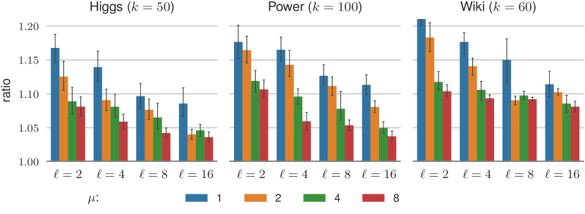
Figure 2. Approximation ratio attained by the MapReduce algorithm for $k$-center using coresets of size $\mu k$, with $\mu=1,2,4,8$, and parallelism $\ell=2,4,8,16$.

We first evaluated the MapReduce algorithm for the $k$-center problem, presented in Subsection 3.1, aiming at assessing the impact of the coreset size on the quality of the returned solution. For simplicity, rather than varying the precision parameter $\varepsilon$, we varied the size of the coreset $T_{i}$ extracted from each partition $S_{i}$, setting it to the same value $\tau=\mu k$ for all $i$, with $\mu=1,2,4,8$. Note that for $\mu=1$ the algorithm corresponds to the one in (MalkomesKCWM15, ). We fixed $k=50$ for the Higgs dataset, $k=100$ for the Power dataset, and $k=60$ for the Wiki dataset. These values of $k$, determined through a number of experiments (omitted for brevity) have been chosen as reasonable values marking the beginning of a plateau in the radius of the clustering induced by the returned centers. The plot in Figure 2 reports the approximation ratio attained by the algorithm for different coreset sizes and degrees of parallelism. As implied by the theory, the solution quality improves noticeably as the size of the coreset (regulated by $\mu$) increases. Moreover, the experiments show that, with respect to the algorithm by (MalkomesKCWM15, ) (blue bar in the plot), even a moderate increase in the coreset size yields a sensibly better solution. This behavior is observed also on the Wiki dataset, which, given its high dimensionality, is a difficult input for our algorithm. In these experiments, the running times, not reported for brevity, exhibited essentially a linear behavior in $\tau$, for fixed parallelism, but remained tolerable (under one minute) even for $\tau=8k$ and parallelism $\ell=2$. Considering also the scalability of the algorithm, which will be assessed in Subsection 5.3, we can conclude that using larger coresets can yield better solution quality at a tolerable performance penalty. From the figure, we finally observe that increasing the parallelism $\ell$ also leads to better solutions, which is due to the fact that the size $\ell\cdot\tau$ of the aggregated coreset $T$ on which gmm is run in the second round, increases.

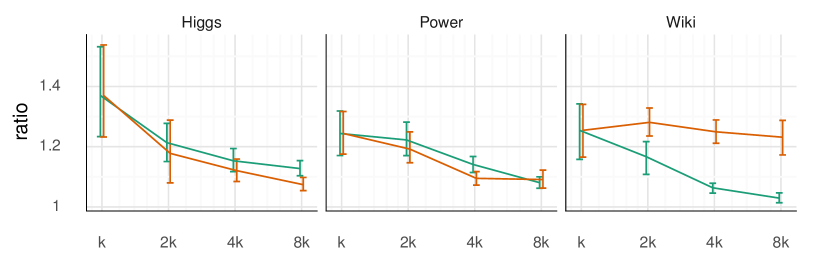
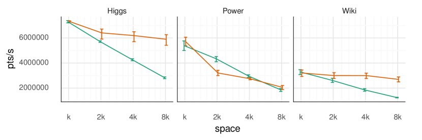
Figure 3. Approximation ratio (top) and throughput (bottom) versus space for the CoresetStream (in orange) and BaseStream (in green) $k$-center streaming algorithms. CoresetStream uses space $\mu\cdot k$, with $\mu=1,2,4,8,16$, BaseStream requires space $m\cdot k$, with $m=1,2,4,8,16$ ($\mu$ and $m$ increase from left to right in each plot).

For what concerns the Streaming setting, as observed in Section 4, our coreset approach would yield an algorithm matching the approximation quality of the state-of-the-art $(2+\varepsilon)$-approximation algorithm by (McCutchen2008, ). Nonetheless, we performed a number of experiments to compare the practical performance of the two algorithms. The results, reported in Figure 3, show that the algorithm by (McCutchen2008, ) (dubbed BaseStream) makes slightly better use of the available space, although our algorithm (dubbed CoresetStream) often exhibits higher throughput while yielding similar approximation quality.

5.2. $k$-center with outliers

To evaluate our algorithms for the $k$-center problem with $z$ outliers, we artificially injected outliers into the datasets as follows. For each dataset, we first determined radius $r_{\mbox{\tiny MEB}}$ and center $c_{\mbox{\tiny MEB}}$ of its Minimum Enclosing Ball (MEB). Then, we added $z=200$ points at distance $100\cdot r_{\mbox{\tiny MEB}}$ from the $c_{\mbox{\tiny MEB}}$ in random directions. By doing so, each added point is at distance $\geq 99\cdot r_{\mbox{\tiny MEB}}$ from any point in the dataset. Furthermore, we verified that the minimum distance between any two added points is $\geq 10\cdot r_{\mbox{\tiny MEB}}$, making these points true outliers.

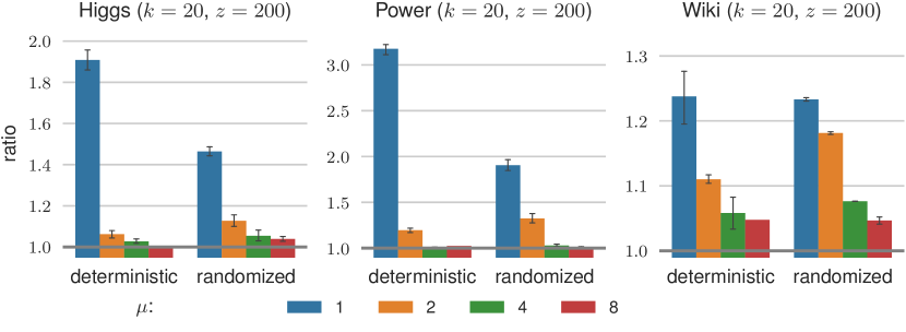
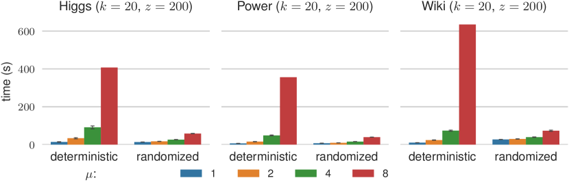
Figure 4. Approximation ratio (top) and running time (bottom) attained by the deterministic and randomized MapReduce algorithms for the $k$-center with $z$ outliers problem, using coresets of size $\mu(k+z)$ and $\mu(k+6\cdot z/\ell)$, respectively, with $\mu=1,2,4,8$, and fixed parallelism $\ell=16$.

A first set of experiments was run to compare the deterministic and randomized versions of our algorithm presented in Subsection 3.2 against each other and against the algorithm in (MalkomesKCWM15, ). We set $k=20$ and $z=200$ for both datasets and fixed the parallelism to $\ell=16$. Also, we partitioned the data adversarially, placing all outliers in the same partition so to better test the benefits of randomization. As before, rather than regulating the size of each coreset $T_{i}$ through the precision parameter, we fixed it equal to $\tau$ for each $i$, setting $\tau=\mu(k+z)$ for the deterministic algorithm, and $\tau=\mu(k+6\cdot z/\ell)$ for the randomized one, with $\mu=1,2,4,8$. Again, the deterministic algorithm with $\mu=1$ coincides with the algorithm by (MalkomesKCWM15, ). Based on Lemma 10, the term $6\cdot z/\ell$ in the value of $\tau$ for the randomized algorithm is meant to upper bound the number of outliers included in each partition (ignoring the logarithmic factor which is needed to ensure high probability only when $z\simeq\ell$).

Figure 4 reports the results of these experiments. As before, we note that the quality of the solution improves noticeably with the coreset size (regulated by $\mu$) and even a moderate increase in the coreset size yields a significant improvement with respect to the baseline of (MalkomesKCWM15, ), represented by the blue column ($\mu=1$, deterministic). In particular, when $\mu=1$ the coreset extracted from the partition containing all outliers is forced to include the outliers, hence few other centers can be selected to account for the non-outlier points in the partition, which are thus underrepresented. In this case, the randomized algorithm, where the number of outliers per partition is smaller and slightly overestimated by the constant 6, attains a better solution quality. As the coreset size increases, there is a sharper improvement of the quality of the solution found by the deterministic algorithm, since there are now enough centers to well represent the non-outlier points, even in the partition containing all outliers, while in the randomized algorithm, the effect of the coreset size on the quality of the solution is much smoother. Nevertheless, for $\mu>1$, the randomized algorithm finds solutions of comparable quality to the ones found by the deterministic algorithm, using much smaller coresets. For what concerns the running time, the bottom plots of Figure 4 clearly show that the reduction in the coreset size featured by the randomized algorithm yields high gains in performance, providing evidence that this algorithm can attain much better solutions than (MalkomesKCWM15, ) with a comparable running time.

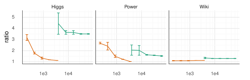
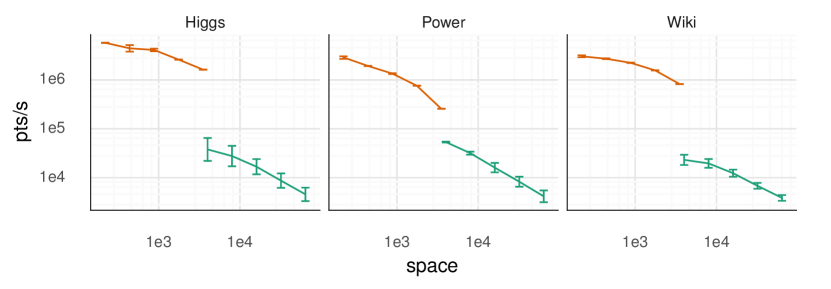
Figure 5. Approximation ratio (top) and throughput (bottom) versus space for CoresetOutliers (in orange) and BaseOutliers (in green). CoresetOutliers uses space $\mu(k+z)$, with $\mu=1,2,4,8,16$, BaseOutliers requires space $m(k\cdot z)$, with $m=1,2,4,8,16$ ($\mu$ and $m$ increase from left to right in each plot). Space and throughput are in logarithmic scale.

In a second set of experiments, we studied the impact of the coreset size on the quality of the solution computed by the Streaming algorithm presented in Section 4 (dubbed CoresetOutliers) and compared its performance with the state-of-the-art algorithm of (McCutchen2008, ) (dubbed BaseOutliers) which essentially runs a number $m$ of parallel instances of a $(k\cdot z)$-space Streaming algorithm, where $m$ depends on the desired approximation target. We used the same datasets and the same input parameters ($k=20$ and $z=200$) as in the previous experiment. The points are shuffled before being streamed to the algorithms. Since the two algorithms feature different parameters, we compare their performance as a function of the amount of space used, which is $\mu(k+z)$ (i.e., the coreset size) for CoresetOutliers, and $m(k\cdot z)$ for BaseOutliers. The results are reported in Figure 5. We observe that for Higgs and Power CoresetOutliers yields better approximation ratios than BaseOutliers using considerably less space, which is coherent with the better theoretical quality featured by the former algorithm. For both algorithms, using more resources (i.e., larger values of $\mu$ and $m$, respectively) leads to better quality solutions, with CoresetOutliers approaching the best quality ever attained (approximation ratio almost 1). As for Wiki, we note that both algorithms already yield very good solutions with minimum space, which implies that for this dataset larger space does not provide significant quality improvements. This is probably an effect of the high dimensionality of the dataset. To assess efficiency, we considered throughput, i.e., the number of points processed per second by the algorithm ignoring the cost of streaming data from memory. As expected, for both CoresetOutliers and BaseOutliers throughput is inversely proportional to the space used. However, by comparing the top and bottom graphs for each dataset, it can be immediately seen that for a fixed approximation ratio, CoresetOutliers uses less space and exhibits a throughput substantially higher (always more than 1 order of magnitude). Thanks to its high throughout, even for large values of $\mu$, CoresetOutliers is able to keep up with real-world streaming pipelines (e.g., in 2013 Twitter peaked at 143,199 tweets/s (TwitterThroughput, )).

5.3. Scalability of the MapReduce algorithms

For brevity, we focus on the randomized MapReduce algorithm for the $k$-center problem with $z$ outliers, since the results for the other cases are similar. A first set of experiments was run to assess the scalability with respect to the input size. To this end, we generated synthetic instances of the Higgs, Power, and Wiki datasets, $h$ times larger than the original datasets, with $h=25,50$ and 100. We used the following generation process. Starting with the original dataset, a random point is sampled, and each of its coordinates is modified through the addition of a Gaussian noise term with mean 0 and standard deviation which is $10\%$ of the difference between the maximum and the minimum value of that coordinate across the original dataset. This perturbed point is then added to the synthetic dataset until the desired size is reached. The rationale behind this construction is to build a (much larger) synthetic dataset with the same clustered structure as the original one, similarly to the SMOTE technique used in machine learning to combat class imbalance (ChawlaBHK02, ). Also, outliers have been added to each generated instance, as detailed in the previous subsection. On each instance of the datasets we ran the randomized MapReduce algorithm with $k=20$, $z=200$, using maximum parallelism ($\ell=16$) and setting the size of each coreset $T_{i}$ to $8*(k+6\cdot z/\ell)$. Figure 6 plots the running times (averages of 10 runs) and shows that the algorithm scales linearly with the input size.

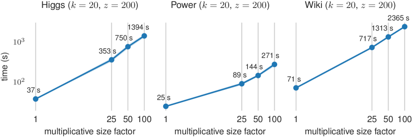
Figure 6. Scalability with respect to input size of the randomized MapReduce algorithm for the $k$-center problem with $z$ outliers, using coresets of size $8\cdot(k+6\cdot z/\ell)$ and parallelism 16. Both axes are in logarithmic scale.

We ran a second set of experiments to assess the scalability of the algorithm with respect to the number of processors. For these experiments, we used the original datasets with added outliers, setting $k=20$ and $z=200$, as before. In order to target the same solution quality over all runs, we fixed the size of the union of the coresets, from which OutliersCluster extracts the final solution, equal to $8(16k+6z)$, which corresponds to the case $\mu=8$ and $\ell=16$ of Figure 4. Then, we ran the algorithm varying the parallelism $\ell$ between $1$ and $16$, setting, for each value of $\ell$, the size of each $T_{i}$ to $\tau_{\ell}=8(16k+6z)/\ell$, so to obtain the desired size for the union. Figure 7 plots the running times distinguishing between the time required by the coresets construction (orange area) and the time required by OutliersCluster (blue area). While the latter time is clearly constant, coreset construction time, which dominates the running time for small $\ell$, scales superlinearly with the number of processors. In fact, doubling the parallelism results in about a 4-fold improvement of the running time up to 8 processors, since each processor performs work proportional to $\tau_{\ell}\cdot|S|/\ell$, and $\tau_{\ell}$ embodies an extra factor $\ell$ in the denominator. This effect is milder going from 8 to 16 processors because of the overhead of initial random shuffle of the data.

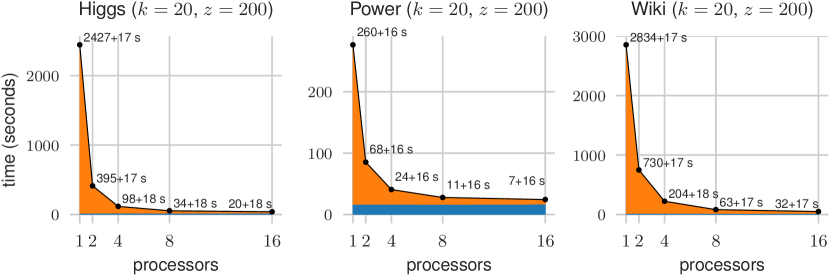
Figure 7. Scalability with respect to the number of processors of the randomized MapReduce algorithm for the $k$-center problem with $z$ outliers, using coresets of size $8*(16k+6z)$ and parallelism $\ell=1,2,4,8,16$. Each point is labeled with the sum of the time required to build the coreset (orange area) and the time required to compute the final solution on the coreset (blue area).

5.4. Improved sequential performance

As we discussed in Section 3, for the $k$-center problem with $z$ outliers we can improve on the superquadratic complexity of the state of the art algorithm in (Charikar2001, ), which we dub CharikarEtAl in the following, by running our deterministic MapReduce algorithm sequentially, at the expense of a slightly worse approximation guarantee. (In fact, the CharikarEtAl algorithm amounts to $O\left(\log|S|\right)$ executions of our OutliersCluster with $\hat{\varepsilon}=0$ and unit weights on the entire input $S$.) To quantify the achievable gains, we took a sample of 10000 points from each dataset (so to keep CharikarEtAl’s running time within feasible bounds). As before, we injected 200 outliers, using the same procedure outlined above, and set $k=20$ and $z=200$. We ran our MapReduce algorithm with $\ell=1$ (indeed, for $\ell=1$, the algorithm is sequential) and $\mu=1,2,4,8$. Figure 8 reports, for the three datasets, the running times (top plots) and the radii of the returned clusterings (bottom plot) for CharikarEtAl and our algorithm for varying $\mu$. Measures are averages over 10 runs, with the input dataset shuffled before each run. Note that the case $\mu=1$ corresponds to the algorithm in (MalkomesKCWM15, ), therefore we label it as MalkomesEtAl

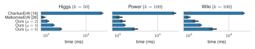
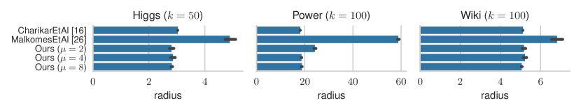
Figure 8. Running time (top, in logarithmic scale) and radius (bottom) of different sequential algorithms on a sample of 10 thousands points of Higgs, Power, and Wiki.

From the figure it is clear that building a coreset before running OutliersCluster is highly beneficial for the running time, which improves by one order of magnitude. However, the solution quality for MalkomesEtAl (i.e., $\mu=1$) is much worse than the one featured by CharikarEtAl. In contrast, the bars for $\mu>1$ show that a substantial performance improvement over the one of CharikarEtAl can be attained, while keeping the approximation quality essentially unchanged. Observe that, in some cases, our algorithm returns better radii than CharikarEtAl, even if from the theory one would expect a slightly worse behavior. This is probably due to the fact that while CharikarEtAl is essentially insensitive to shufflings of the data, our coreset construction, based on gmm, introduces an element of arbitrariness with the choice of the initial center, which may result in different coresets for different shuffles, potentially leading to a better average solution quality.

6. Conclusions

We presented MapReduce and Streaming algorithms for the $k$-center problem (with and without outliers) based on flexible coreset constructions. These constructions yield a spectrum of space-accuracy tradeoffs regulated by the doubling dimension $D$ of the underlying space, and afford approximation guarantees arbitrarily close to those of the best sequential strategies, using moderate space in the case of small $D$. The theoretical analysis of the algorithms is complemented by experimental evidence of their practicality.

Coresets provide an effective way of processing large amounts of data by building a succinct summary of the input which can then be processed with the sequential algorithm of choice. In particular, we showed how to leverage coresets to build MapReduce and Streaming algorithms for the $k$-center problem with and without outliers. Building on state-of-the art approaches for these problems, we provide flexible coreset constructions which yield a spectrum of space-accuracy tradeoffs which allow to obtain approximation guarantees that can be made arbitrarily close to those obtainable with the best sequential strategies at the expense of an increase of the memory requirements, regulated by the dimensionality of the underlying metric space. The theoretical findings are complemented by experimental evidence of the practicality of the proposed algorithms.

Future avenues of research include further improvements of the local memory requirements of the MapReduce algorithms, the development of a 1-pass Streaming algorithm oblivious to the doubling dimension $D$ of the metric space, and the extension of our approach to other (center-based) clustering problems.

References

- [1] Twitter Blog: New Tweets per Second Record, and How! https://blog.twitter.com/engineering/en_us/a/2013/new-tweets-per-second-record-and-how.html.
- [2] UCI higgs dataset. https://archive.ics.uci.edu/ml/datasets/HIGGS.
- [3] UCI power dataset. https://archive.ics.uci.edu/ml/datasets/Individual+household+electric+power+consumption.
- [4] P. Agarwal, S. Har-Peled, and K. Varadarajan. Approximating Extent Measures of Points. Journal of the ACM, 51(4):606–635, 2004.
- [5] S. Aghamolaei, M. Farhadi, and H. Zarrabi-Zadeh. Diversity Maximization via Composable Coresets. In Proc. CCCG, 2015.
- [6] A. Assadi and S. Khanna. Randomized Composable Coresets for Matching and Vertex Cover. In Proc. ACM SPAA, pages 3–12, 2017.
- [7] P. Awasthi and M. Balcan. Center based clustering: A foundational perspective. In Handbook of cluster analysis. CRC Press, 2015.
- [8] M. Badoiu, S. Har-Peled, and P. Indyk. Approximate Clustering via Core-sets. In Proc. ACM STOC, pages 250–257, 2002.
- [9] P. Beame, P. Koutris, and D. Suciu. Communication Steps for Parallel Query Processing. In Proc. ACM PODS, pages 273–284, 2013.
- [10] M. Ceccarello, C. Fantozzi, A. Pietracaprina, G. Pucci, and F. Vandin. Clustering Uncertain Graphs. PVLDB, 11(4):472–484, 2017.
- [11] M. Ceccarello, A. Pietracaprina, and G. Pucci. Fast Coreset-based Diversity Maximization under Matroid Constraints. In Proc. ACM WSDM, pages 81–89, 2018.
- [12] M. Ceccarello, A. Pietracaprina, G. Pucci, and E. Upfal. Space and Time Efficient Parallel Graph Decomposition, Clustering, and Diameter Approximation. In Proc. ACM SPAA, pages 182–191, 2015.
- [13] M. Ceccarello, A. Pietracaprina, G. Pucci, and E. Upfal. A Practical Parallel Algorithm for Diameter Approximation of Massive Weighted Graphs. In Proc. IEEE IPDPS, 2016.
- [14] M. Ceccarello, A. Pietracaprina, G. Pucci, and E. Upfal. MapReduce and Streaming Algorithms for Diversity Maximization in Metric Spaces of Bounded Doubling Dimension. PVLDB, 10(5):469–480, 2017.
- [15] M. Charikar, C. Chekuri, T. Feder, and R. Motwani. Incremental Clustering and Dynamic Information Retrieval. SIAM J. on Computing, 33(6):1417–1440, 2004.
- [16] M. Charikar, S. Khuller, D. Mount, and G. Narasimhan. Algorithms for Facility Location Problems with Outliers. In In Proc. ACM-SIAM SODA, pages 642–651, 2001.
- [17] N. Chawla, K. Bowyer, L. Hall, and W. Kegelmeyer. SMOTE: Synthetic Minority Over-sampling Technique. J. Artif. Intell. Res., 16:321–357, 2002.
- [18] J. Dean and S. Ghemawat. MapReduce: Simplified Data Processing on Large Clusters. Communications of the ACM, 51(1):107–113, 2008.
- [19] A. Ene, S. Im, and B. Moseley. Fast Clustering Using MapReduce. In Proc. ACM KDD, pages 681–689, 2011.
- [20] T. Gonzalez. Clustering to Minimize the Maximum Intercluster Distance . Theoretical Computer Science, 38:293–306, 1985.
- [21] C. Hennig, M. Meila, F. Murtagh, and R. Rocci. Handbook of cluster analysis. CRC Press, 2015.
- [22] M. Henzinger, P. Raghavan, and S. Rajagopalan. Computing on Data Streams. In Proc. DIMACS, pages 107–118, 1998.
- [23] S. Im and B. Moseley. Brief Announcement: Fast and Better Distributed MapReduce Algorithms for k-Center Clustering. In Proc. ACM SPAA, pages 65–67, 2015.
- [24] P. Indyk, S. Mahabadi, M. Mahdian, and V. Mirrokni. Composable Core-sets for Diversity and Coverage Maximization. In Proc. ACM PODS, pages 100–108, 2014.
- [25] J. Leskovec, A. Rajaraman, and J. Ullman. Mining of Massive Datasets, 2nd Ed. Cambridge University Press, 2014.
- [26] G. Malkomes, M. Kusner, W. Chen, K. Weinberger, and B. Moseley. Fast Distributed k-Center Clustering with Outliers on Massive Data. In Proc. NIPS, pages 1063–1071, 2015.
- [27] R. McCutchen and S. Khuller. Streaming Algorithms for k-Center Clustering with Outliers and with Anonymity. In Proc. APPROX-RANDOM, pages 165–178, 2008.
- [28] T. Mikolov, I. Sutskever, K. Chen, G. S. Corrado, and J. Dean. Distributed Representations of Words and Phrases and their Compositionality. In Proc. NIPS, pages 3111–3119, 2013.
- [29] M. Mitzemacher and E. Upfal. Probability and Computing. Cambridge University Press, 2nd edition, 2017.
- [30] J. Munro and M. Paterson. Selection and Sorting with Limited Storage. Theor. Comput. Sci., 12:315–323, 1980.
- [31] A. Pietracaprina, G. Pucci, M. Riondato, F. Silvestri, and E. Upfal. Space-Round Tradeoffs for MapReduce Computations. In Proc. ACM ICS, pages 235–244, 2012.
- [32] M. Z. V. Mirrokni. Randomized Composable Core-sets for Distributed Submodular Maximization. In Proc. ACM STOC, pages 153–162, 2015.
- [33] M. Zaharia, M. Chowdhury, M. Franklin, S. Shenker, and I. Stoica. Spark: Cluster Computing with Working Sets. In Proc. USENIX HotCloud, 2010.