Quantum spin ice with frustrated transverse exchange : from $\pi$–flux phase
to nematic quantum spin liquid

Abstract

Quantum spin ice materials, pyrochlore magnets with competing Ising and transverse exchange interactions, have been widely discussed as candidates for a quantum spin–liquid ground state. Here, motivated by quantum chemical calculations for Pr pyrochlores, we present the results of a study for frustrated transverse exchange. Using a combination of variational calculations, exact diagonalisation, numerical linked-cluster and series expansions, we find that the previously-studied $U(1)$ quantum spin liquid, in its $\pi$-flux phase, transforms into a nematic quantum spin liquid at a high–symmetry, $SU(2)$ point.

Pyrochlore magnets have proved an exceptionally rich source of new phenomena Gardner et al. (2010); Hallas et al. (2018), including the classical spin liquid “spin ice” Bramwell and Gingras (2001); Castelnovo et al. (2012), celebrated for its magnetic monopole excitations Castelnovo et al. (2008). Pyrochlore materials also stand at the forefront of the search for quantum spin liquids (QSL), massively–entangled quantum phases of matter, which provide accessible examples of exotic, topological (quasi–)particles previously studied in high–energy physics Balents (2010); Savary and Balents (2017a); Zhou et al. (2017); Norman (2016). In particular, the quantum analogue of spin ice has been shown to support a three–dimensional QSL with fractional excitations, described by a $U(1)$ lattice gauge theory Hermele et al. (2004); Banerjee et al. (2008); Shannon et al. (2012); Benton et al. (2012); Kato and Onoda (2015); Huang et al. , and has been vigorously pursued in experiment Ross et al. (2011); Kimura et al. (2013); Petit et al. (2016); Wen et al. (2017); Martin et al. (2017); Sibille et al. .

Exciting as these developments are, the range of outcomes in experiment remains far broader than predicted by theory Gardner et al. (2010); Hallas et al. (2018). Encouragingly, studies of more general pyrochlore–lattice models, in their classical limit, reveal a variety of new ordered and spin–liquid phases, which may provide insight into experiments carried out at finite temperature Onoda and Tanaka (2011); Benton et al. (2016); Petit et al. (2016); Yan et al. (2017); Taillefumier et al. (2017). However, to date, very little is known about the ground state of even the simplest model of a quantum spin ice for frustrated transverse exchange, where quantum Monte Carlo simulation fails Lee et al. (2012); Chen (2017a). And, since microscopic estimates for Pr–based pyrochlore magnets have predicted frustrated interactions Onoda and Tanaka (2011), this is a question of both fundamental and experimental interest.

In this Letter we address the fate of the QSL in a quantum spin ice with frustrated transverse exchange. We find that the $U(1)$ QSL, in its $\pi$-flux phase Lee et al. (2012), gives way to a new, nematic QSL, at a special $SU(2)$–symmetry point in parameter space. Evidence in support of this claim is taken from exact diagonalisation (ED); a cluster–based mean–field theory (CMFT); cluster–based variational calculations (cVAR); and an exact, variational argument at the $SU(2)$ point. Further evidence for the growth of nematic correlations, and of an unusual scaling of heat capacity at high temperature, are presented through numerical linked–cluster expansion (NLCE) and high–temperature series expansion (HTE) calculations. These results, summarised in Fig. 1, provide a concrete example of a nematic quantum spin liquid Grover et al. (2010), in three dimensions, and confirm that even the simplest models of pyrochlore magnets can support a range of different QSL ground states.

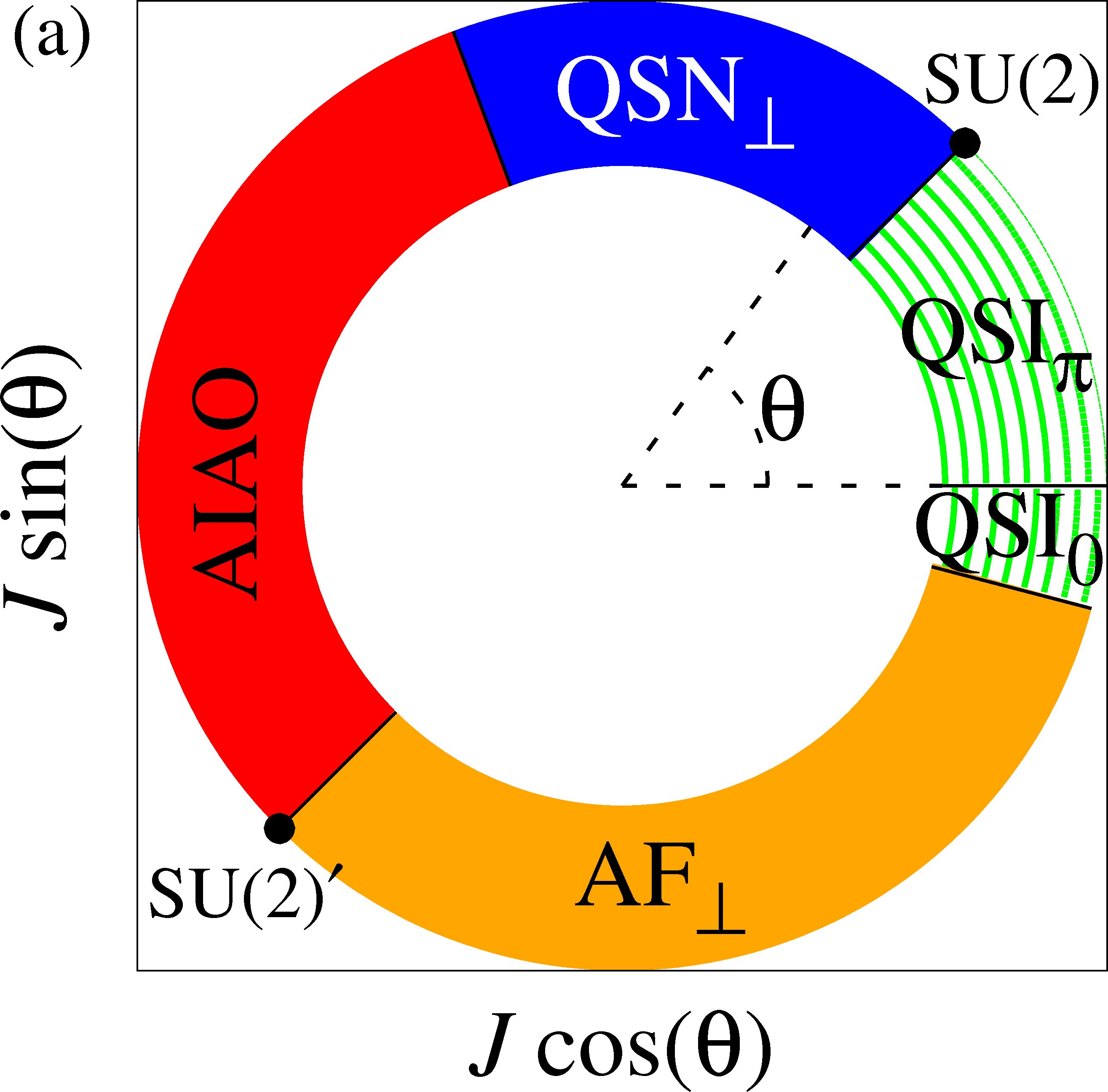
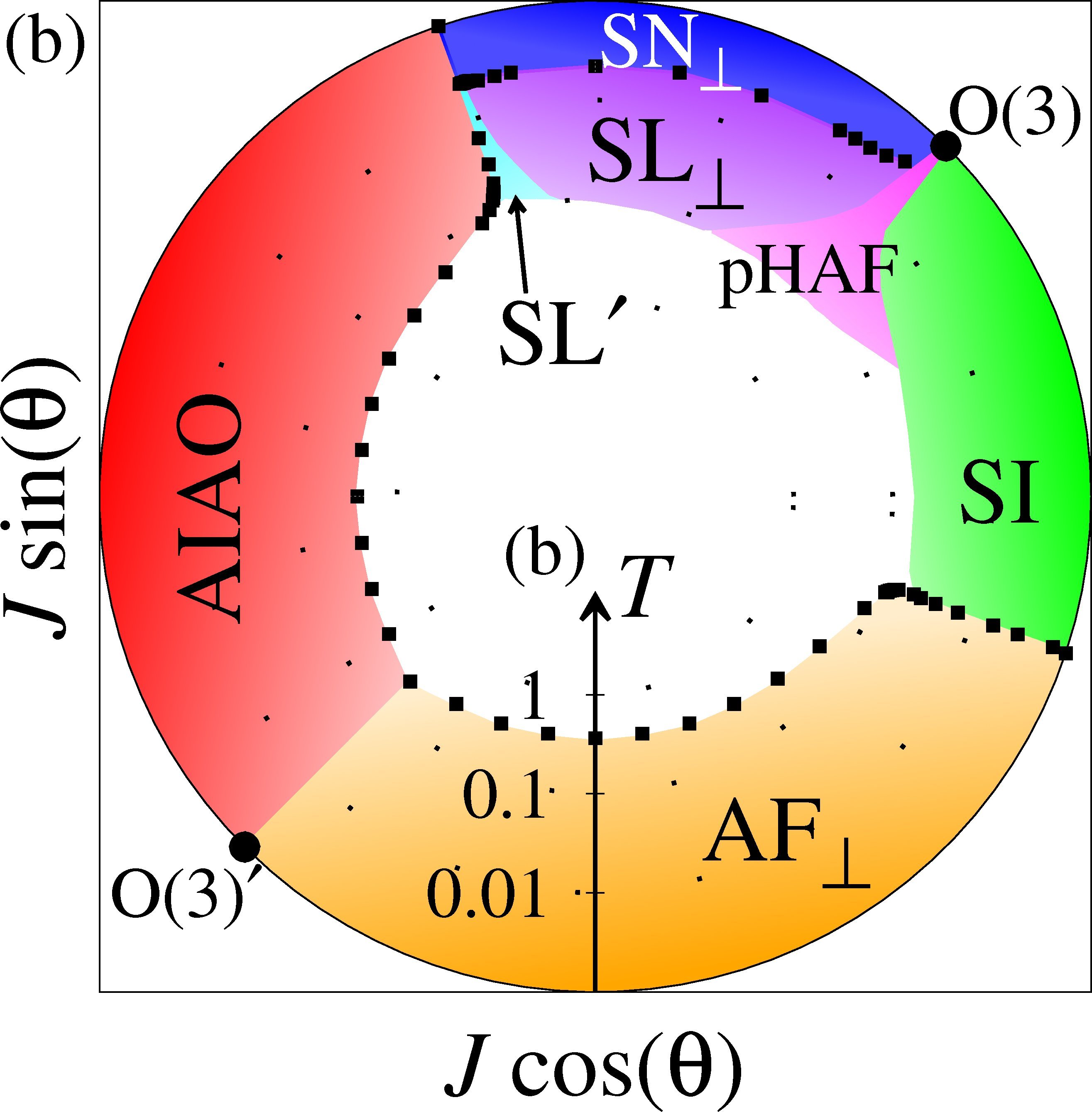
Figure 1: Phase diagram of the quantum spin ice model $\mathcal{H}_{\sf XXZ}$ [Eq. (1), Eq. (2)]: (a) Quantum phase diagram found in cluster–variational (cVAR) calculations for $T=0$. Two quantum spin liquids (QSL) descended from spin ice, QSI₀ and QSI_π, compete with easy–plane antiferromagnetic order (AF_⟂); all–in all-out magnetic order (AIAO); and a nematic QSL (QSN_⟂). QSI_π and QSN_⟂ are connected by a point with $SU(2)$ symmetry. (b) Phase diagram found in classical Monte Carlo simulations for $T>0$ [cf. Ref. Taillefumier et al., 2017]. Three spin liquids; spin ice (SI); the easy–plane spin liquid (SL_⟂); and a pseudo–Heisenberg antiferromagnet (pHAF); compete with a nematic spin liquid (SN_⟂); and AF_⟂ and AIAO order. An additional disordered regime (SL^′) shares the correlations of SL_⟂ and AIAO. Details of simulation methods are given in the Supplemental Materials.

The model we consider is the spin–$1/2$ XXZ Hamiltonian on the pyrochlore lattice

$$\mathcal{H}_{\sf XXZ}=\sum_{\langle ij\rangle}\left[J_{zz}{\sf S}^{z}_{i}{\sf S}^{z}_{j}-J_{\pm}\left({\sf S}^{+}_{i}{\sf S}^{-}_{j}+{\sf S}^{+}_{j}{\sf S}^{-}_{i}\right)\right]$$ (1)

where spin coordinates are defined in a local coordinate frame such that the $z$-axis of spin space is aligned with a local $C_{3}$ axis Ross et al. (2011); Yan et al. (2017). Eq. (1) can be derived from atomic models of pyrochlore oxides Molavian et al. (2007); Onoda and Tanaka (2010, 2011) and, for $J_{zz}\gg J_{\pm}>0$, has been extensively studied as a minimal model of a quantum spin ice Hermele et al. (2004); Banerjee et al. (2008); Shannon et al. (2012); Benton et al. (2012); Kato and Onoda (2015); Huang et al. ; Lee et al. (2012); Chen (2017a); Savary and Balents (2012); Hao et al. (2014); McClarty et al. (2015); Gingras and McClarty (2014); Chen (2016); Shannon (2017); Savary and Balents (2017b); Chen (2017b). Since we are concerned with both positive and negative signs of interaction, it is convenient to write

$$J_{zz}=J\cos\theta\quad,\quad J_{\pm}=-\frac{J}{2}\sin\theta\;.$$ (2)

At the special points $\theta=\pi/4$, and $\theta=-3\pi/4$, $\mathcal{H}_{\sf XXZ}$ is equivalent to a Heisenberg model, and has an $SU(2)$ symmetry.

For unfrustrated interactions, $-\pi/2<\theta<0$, $\mathcal{H}_{\sf XXZ}$ [Eq. (1)] is accessible to quantum Monte Carlo (QMC) simulation. In this case, for $\theta\lesssim 0$, the ground–state is known to be a $U(1)$ QSL (QSI₀), giving way to an easy–plane antiferromagnet (AF_⟂) for $\theta<-0.05$ Banerjee et al. (2008); Shannon et al. (2012); Kato and Onoda (2015). Perturbative arguments imply that the $U(1)$ QSL should also survive for frustrated interactions, $\theta\gtrsim 0$ Hermele et al. (2004). In this case the $U(1)$ QSL enters a “$\pi$–flux phase” (QSI_π), in which its topological, spinon excitations have a modified dispersion, due to a fractionalisation of translational symmetry Lee et al. (2012); Chen (2017a). Classical Monte Carlo simulations suggest that $\mathcal{H}_{\sf XXZ}$ remains in a spin liquid state for $0<\theta<1.89$, but that this spin liquid changes its character traversing the high–symmetry point $\theta=\pi/4$ Taillefumier et al. (2017) — cf. Fig. 1(b). The fate of the quantum, $\pi$–flux ground state, however, remains unknown.

CMFT– In order to shed light on this question, we first explore the ground state of $\mathcal{H}_{\sf XXZ}$ [Eq. (1)] within an approach based on cluster mean field theory (CMFT). CMFT consists in breaking the lattice up into finite clusters and treating the interactions within each cluster exactly, while those between clusters are treated at a mean–field level García-Adeva and Huber (2000, 2001); Shannon (2002); Yamamoto et al. (2014); Javanparast et al. (2015). The geometry of the pyrochlore lattice permits degenerate CMFT solutions, with translational symmetry restored, in contrast to some previous approaches (see e.g. Yamamoto et al. (2015)), allowing us to treat spin–liquid states.

We start by dividing the pyrochlore lattice into two sublattices of tetrahedra, ‘A’ and ‘B’, and writing the wave function as a product over A–sublattice tetrahedra

$$|\psi^{\sf CMFT}(\{{\bf h}\})\rangle=\Pi_{t\in A}|\phi_{t}(\{{\bf h}\})\rangle\;,$$ (3)

where $|\phi_{t}(\{{\bf h}\})\rangle$ is defined as the ground state of an auxiliary Hamiltonian on tetrahedron $t$

$$\mathcal{H}^{\prime}(t)=\mathcal{H}_{\sf XXZ}(t)-\sum_{i\in t}{\bf h}_{i}\cdot{\sf S}_{i}\;.$$ (4)

Correlations within B–sublattice tetrahedra are treated at a mean–field level, through the self–consistently determined field $\{{\bf h}\}$

$$\mathcal{H}^{\prime}(t)|\phi_{t}(\{{\bf h}\})\rangle=\epsilon_{t}|\phi_{t}(\{{\bf h}\})\rangle\;,$$ (5)

with the optimal values of $\{{\bf h}\}$ found variationally, by minimising

$$E_{\sf CMFT}=\langle\psi^{\sf CMFT}(\{{\bf h}\})|\mathcal{H}_{\sf XXZ}|\psi^{\sf CMFT}(\{{\bf h}\})\rangle\;.$$ (6)

The corner–sharing geometry of the pyrochlore lattice permits solutions for a single tetrahedron to be connected in many different ways (cf. “lego–brick rules” in Yan et al. (2017)). For this reason the solution for $\{{\bf h}\}$, and the corresponding wave function $|\psi^{\sf CMFT}(\{{\bf h}\})\rangle$, encompass disordered as well as ordered states.

We find four kinds of optimal solutions for the fields ${\bf h}_{i}$, each corresponding to a different region of the phase diagram Fig. 1(a). For $5\pi/4<\theta<1.927$, the optimal solution has ${\bf h}_{i}=h\hat{{\bf z}}$ on all sites, and corresponds to all–in, all–out (AIAO) order. Meanwhile, for $-\frac{3\pi}{4}<\theta\lesssim-0.256$ fields ${\bf h_{i}}$ are globally ordered in the local $xy$ plane, with (e.g.) ${\bf h}_{i}=h\hat{{\bf x}}$. This is the easy–plane antiferromagnet, AF_⟂.

For $-0.256\lesssim\theta<\frac{\pi}{4}$ the optimal solutions are spin–ice–like. The fields ${\bf h}_{i}$ have the form ${\bf h}_{i}=\sigma_{i}h\hat{{\bf z}}$ where $\sigma_{i}=\pm 1$. The minimum value of $E_{\sf CMFT}$ is attained by any configuration of $\sigma_{i}$ with two ‘+’ signs and two ‘-’ signs on every tetrahedron of the lattice. It is known from perturbative arguments that quantum tunnelling between spin–ice configurations gives rise to two distinct $U(1)$ QSL, depending on the sign of $J_{\pm}$ Lee et al. (2012); Chen (2017a). These two phases, QSI₀ and QSI_π, cannot be distinguished within CMFT, but do appear as distinct phases in more sophsticated variational calculations, discussed below.

For $\frac{\pi}{4}\lesssim\theta<1.927$ the optimal solutions are similar to the spin–ice case but now have the fields ${\bf h}_{i}$ lying in the $xy$ plane, in a collinear fashion, e.g. ${\bf h}_{i}=\sigma_{i}h\hat{{\bf x}}$. Once again $E_{\sf CMFT}$ is minimized by any configuration of $\sigma_{i}$ with two ‘+’ signs and two ‘-’ signs on every tetrahedron. Since these $\sigma_{i}$ are disordered, the resulting state does not possess any conventional magnetic order. None the less, the selection of a global axis in the $xy$ plane implies that it breaks the $U(1)$ spin–rotation symmetry of Eq. (1). And this is reflected in a finite value of the spin–nematic order parameter

$$\mathcal{Q}_{\perp}=\bigg{\langle}\frac{1}{3N}\sum_{\langle ij\rangle}\begin{pmatrix}{\sf S}^{x}_{i}{\sf S}^{x}_{j}-{\sf S}^{y}_{i}{\sf S}^{y}_{j}\\ {\sf S}^{x}_{i}{\sf S}^{y}_{j}+{\sf S}^{y}_{i}{\sf S}^{x}_{j}\end{pmatrix}\bigg{\rangle}\;,$$ (7)

defined on the bonds $\langle ij\rangle$ of the pyrochlore lattice Taillefumier et al. (2017).

cVAR– The CMFT wave function, Eq. (3), is entangled at the level of a single tetrahedron, and can describe disordered as well as ordered states. But, it cannot capture the long–range entanglement of a QSL. For this reason, distinguishing the quantum ground states of Eq. (1) requires going beyond mean–field theory. To this end, we now introduce a cluster–variational (cVAR) approach, based on a coherent superposition of the degenerate ground states found in CMFT. We apply this method to the case where CMFT predicts spin–nematic order, finding that quantum fluctuations beyond CMFT lead to a $U(1)$ QSL, which retains spin–nematic order. Further details of the cVAR approach, including its application to the two QSLs descended from spin ice, QSI₀ and QSI_π, can be found in the Supplementary Materials.

We take as a starting point the CMFT ansatz for a spin–nematic state with axis of collinearity ${\bf h}\parallel\hat{{\bf x}}$. A superposition of such wave functions can be written as

$$|\varphi\rangle=\sum_{\{\sigma\}}a_{\{\sigma\}}|\psi^{\sf CMFT}(h\sigma_{i}\hat{\bf x})\rangle\;,$$ (8)

where the sum runs over all Ising configurations $\{\sigma\}$ with two ‘+’ and two ‘-’ on every tetrahedron. The complex coefficients $a_{\{\sigma\}}$ are the variational parameters with which we can further optimize the energy

$$E_{\sf cVAR}=\frac{\langle\varphi|\mathcal{H}_{\sf XXZ}|\varphi\rangle}{\langle\varphi|\varphi\rangle}\;.$$ (9)

The wavefunctions $|\psi^{\sf CMFT}(h\sigma_{i}\hat{\bf x})\rangle$ labelled by different Ising configurations $\{\sigma\}$ are not generally orthogonal. The overlap between different mean–field solutions can be parameterised by a dimensionless quantity $\mu(\theta)$, with $|\mu(\theta)|<1$ The overlap between two optimized CMFT wavefunctions is then $\sim\mu^{N_{\sf diff}}$ where $N_{\sf diff}$ is the number of ‘A’ tetrahedra on which the arrangement of $\sigma_{i}$ differs between the two. Using this fact we can expand both numerator and denominator of Eq. (9) in powers of $\mu$. When $|\mu|\ll 1$, we may justify keeping only the leading term which reduces Eq. (9) to

$$E_{\sf cVAR}\approx E_{\sf CMFT}+\sum_{\{\sigma\},\{\sigma^{\prime}\}}M_{\{\sigma\}\{\sigma^{\prime}\}}a^{\ast}_{\{\sigma^{\prime}\}}a_{\{\sigma\}}\quad$$ (10)

where the matrix element $M_{\{\sigma\}\{\sigma^{\prime}\}}$ is a constant $\propto\mu^{2}$ for two configurations connected by reversing the signs of $\sigma_{i}$ around a single hexagonal plaquette, and zero otherwise.

It follows that minimizing the variational energy in Eq. (10) is equivalent to finding the ground state of the ring–exchange Hamiltonian studied using QMC in Shannon et al. (2012), where the outcome is a $U(1)$ QSL. This implies that the optimal superposition of CMFT wave functions, $|\phi\rangle$ [Eq. (8)], is also a $U(1)$ QSL. Moreover, since each of these mean–field solutions has the same value of $\mathcal{Q}_{\perp}$ [Eq. (7)], this $U(1)$ QSL retains the spin–nematic order found in CMFT. Following Grover et al. (2010), we dub this phase a “nematic quantum spin liquid”, and denote it QSN_⟂ in Fig. 1(a). Evaluating $\mu(\theta)$ numerically, we find $|\mu(\theta)|<0.5$ for all relevant parameters, with $|\mu(\theta)|\to 0.15$ approaching AIAO order. This suggests that the perturbative expansion of Eq. (9) is justified.

Further support for nematic order– We now provide two further arguments, completely independent of the cVAR approach, which support the existence of spin–nematic order.

The first argument is based on approaching the $SU(2)$ point $\theta=\frac{\pi}{4}$ from the small $\theta$ side. For small $\theta>0$ the ground state is the $\pi$-flux $U(1)$ QSL Hermele et al. (2004); Lee et al. (2012); Chen (2017a) (QSI_π in Fig. 1(a)). Gauge Mean Field Theory predicts this state to be stable up to $\theta\approx 1.12$, well beyond the $SU(2)$ point. However, we show below that if QSI_π is stable up to the $SU(2)$ point, it must at that point become unstable to nematicity.

To see this, we observe that an appropriate trial wavefunction for the spin–nematic phase can be generated by taking a ground state wavefunction from within the QSI_π phase and acting on it with global spin rotations:

$$|\text{nem}(\psi)\rangle=\mathcal{R}_{z}(\psi)\mathcal{R}_{y}\left(\frac{\pi}{2}\right)|\text{QSI}_{\pi}\rangle\;,$$ (11)

where $\mathcal{R}_{\alpha}(\phi)$ denotes a global rotation by an angle $\phi$, around the $\alpha$ axis of spin space. The wavefunction $|\text{nem}(\psi)\rangle$ generically supports a finite value of the nematic bond order parameter $\mathcal{Q}_{\perp}$ [Eq. (7)], with all dipolar expectation values vanishing. The angle $\psi$ parameterises the direction of $\mathcal{Q}_{\perp}$ in the nematic state.

Eq. (11) links a wavefunction describing the spin nematic phase with a wavefunction describing QSI_π, using global spin rotations. These spin rotations become symmetries of the model at the $SU(2)$ point $\theta=\frac{\pi}{4}$. Thus, if QSI_π is stable up to the $SU(2)$ point, the energy gap between this state and the spin nematic must vanish there, indicating an incipient instability to nematicity. It follows that the resulting spin–nematic state inherits both the gauge symmetry and the fractionalised translational symmetry of QSI_π.

The argument above cannot, however, rule out the possibility that some other ground state may take over from QSI_π before $\theta=\frac{\pi}{4}$, and have yet lower energy. Such alternative competing ground states around $\theta=\frac{\pi}{4}$ could include various dimer-ordered Harris et al. (1991); Berg et al. (2003); Tsunetsugu (2001a, b); Moessner et al. (2006) and spin liquid Canals and Lacroix (1998, 2000); Kim and Han (2008); Burnell et al. (2009) ground states suggested for the Heisenberg model previously. It is useful therefore to have an alternative way to establish nematic order. This is provided by considering the excitations of the AIAO ordered phase found for $J^{zz}<0$ [cf. Fig. 1(a)].

In the AIAO phase the ground state wavefunction is simply the polarized state with maximum total $S^{z}$. Since total $S^{z}$ is a conserved quantity, the excitations of the AIAO phase can be labelled by the number of spin flips, $\delta S^{z}$, relative to the AIAO ground state.

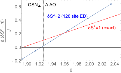
Figure 2: Condensation of two–magnon bound states within the AIAO phase, indicating the onset of spin–nematic order. The gaps to the lowest 1–magnon and 2–magnon excitations of the AIAO phase, $\Delta(\delta S^{z}=1)$ and $\Delta(\delta S^{z}=2)$, are shown as a function of the Hamiltonian parameter $\theta$ [Eq. (2)]. For $\delta S^{z}=1$ the gap has been calculated exactly, while for $\delta S^{z}=2$ it has been estimated numerically for a cluster of 128 spins. As $\theta$ decreases towards $\theta=1.92$ the two–magnon state comes below the one magnon state and then crosses the AIAO state energy. The condensation of two–magnon bound states is a clear indication of incipient nematic order Shannon et al. (2006). This estimate of the phase boundary between QSN_⟂ and AIAO, $\theta\approx 1.924$, is very close to that found in cVAR $\theta\approx 1.927$ [cf. Fig. 1(a)], shown here as a vertical dashed line.

Starting from the AIAO state, an instability to a conventional XY ordered state would be indicated by the softening of a $\delta S^{z}=1$ excitation- i.e. a magnon. An instability to nematic order, by contrast, would be indicated by the softening of a $\delta S^{z}=2$ excitation: a two-magnon bound state Shannon et al. (2006).

The Hamiltonian in the $\delta S^{z}=1$ sector is simply a bosonic hopping Hamiltonian and can be solved exactly. For $\sin(\theta)>0$ the lowest energy state with $\delta S^{z}=1$ has an energy gap $\Delta(\delta S^{z}=1)=J(-3\cos(\theta)-\sin(\theta))$.

In Fig. 2, this energy is compared with the lowest energy state of the $\delta S^{z}=2$ sector, calculated using ED on a 128-site cubic cluster with periodic boundary conditions. Starting from the AIAO phase and approaching the boundary with the proposed nematic QSL we see that the energy of the $\delta S^{z}=2$ sector comes below the energy of the $\delta S^{z}=1$ sector. This indicates the formation of a two–magnon bound state with lower energy than the lowest single–magnon state. The two–magnon bound state crosses the AIAO state at $\theta\approx 1.92$, indicating an instability to nematic order. This is in good agreement with the phase boundary $\theta\approx 1.93$ found using cVAR [Fig. 1(a)].

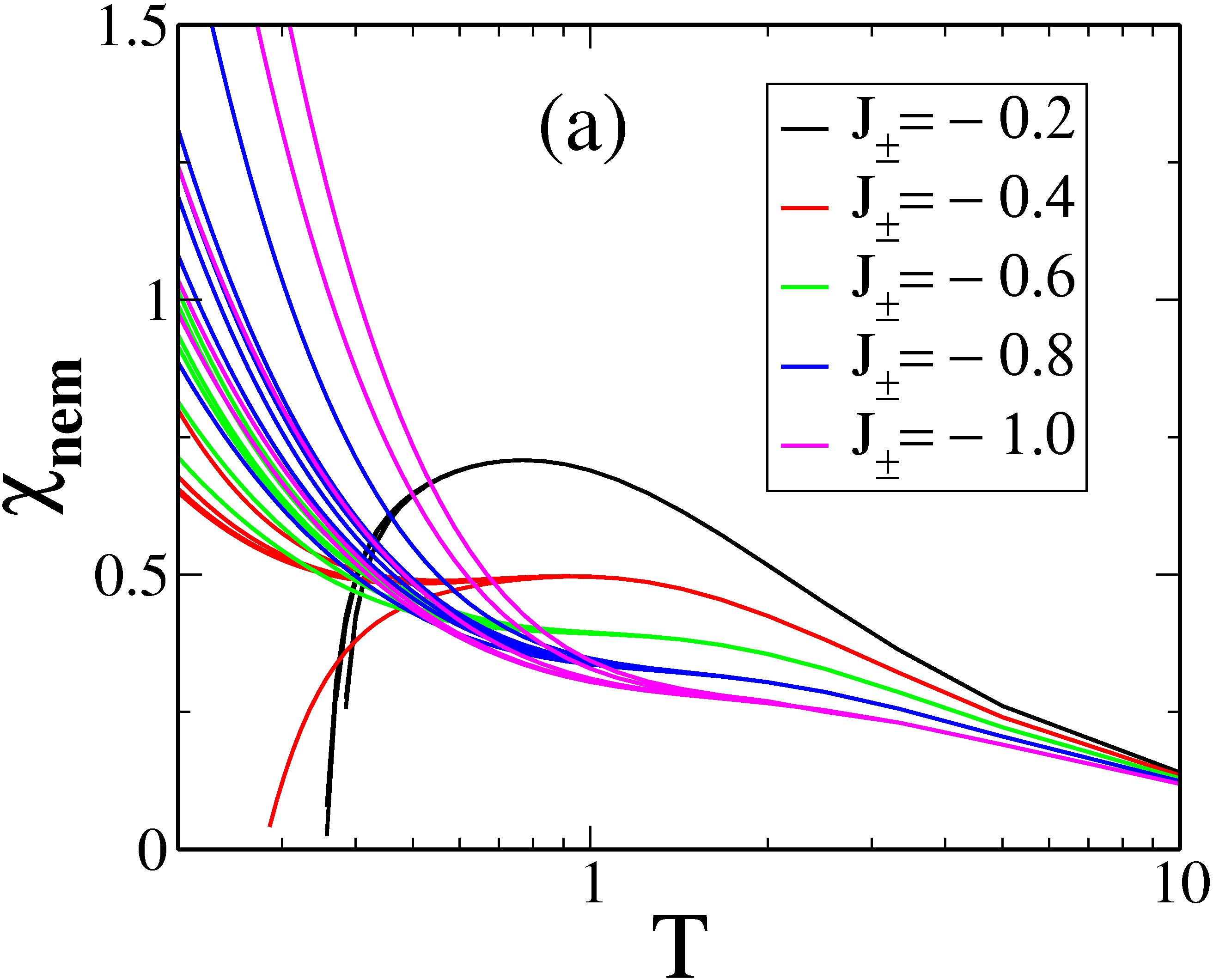
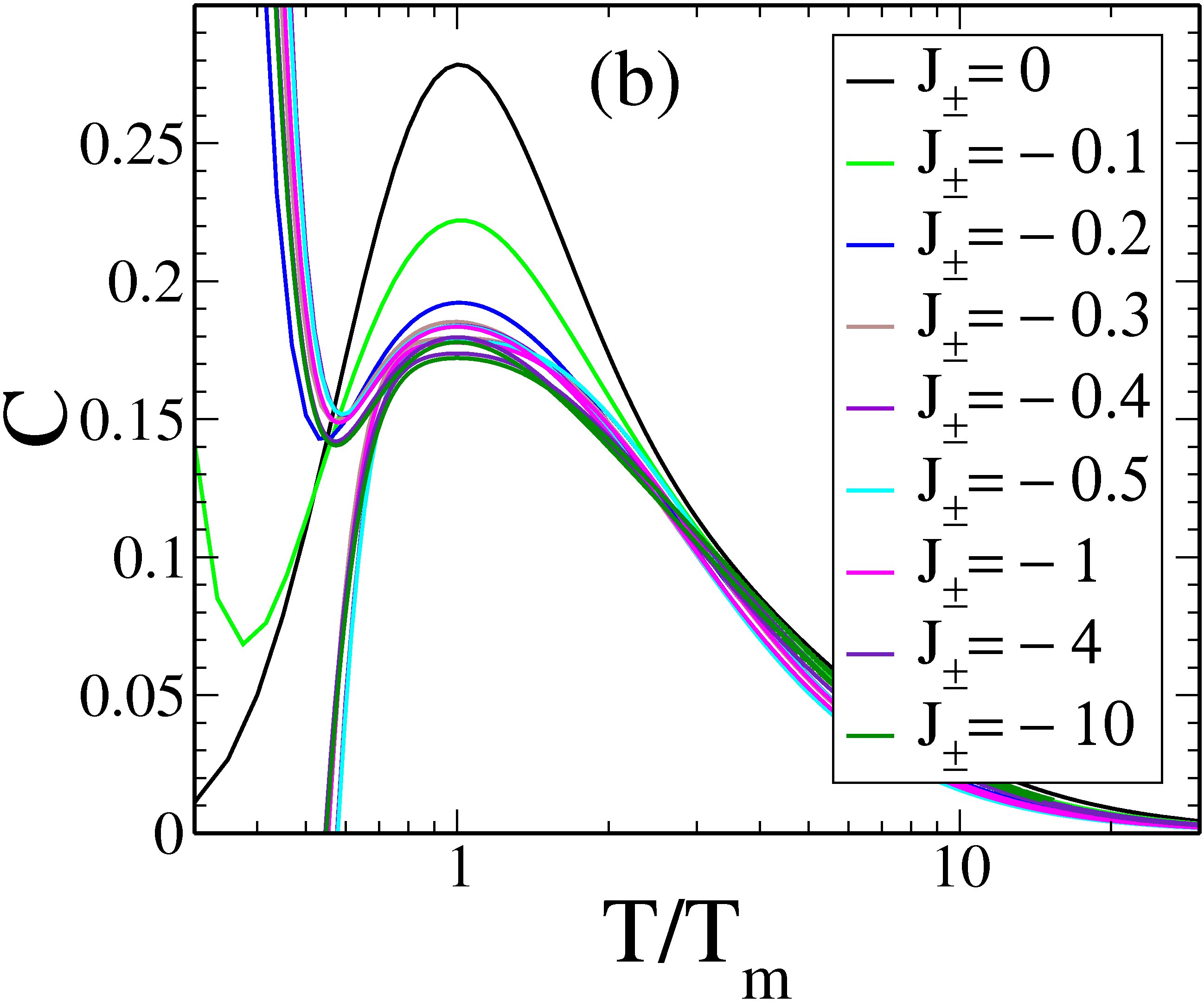
Figure 3: Finite–temperature properties of frustrated quantum spin ice [Eq. 1], calculated for $J_{zz}=1$. (a) Susceptibilty $\chi_{\sf nem}(T)$ associated with spin–nematic order [Eq. (7)], calculated using high–temperature series expansion (HTE). Different curves for a given value of $J_{\pm}$ correspond to different Padé approximants. For $J_{\pm}<-0.5$, $\chi_{\sf nem}(T)$ shows an upturn at low temperatures, consistent with an approach to spin–nematic order. (b) Heat capacity $C$, as a function of reduced temperature $T/T_{m}$, calculated within a numerical linked–cluster expansion (NLCE). Here $T_{m}$ reflects the temperature at which the heat capacity takes on its maximum value for a given value of $J_{\pm}$; different curves for the same value of $J_{\pm}$ represent different orders of NLCE; agreement between these indicates convergence. Plots of $C(T/T_{m})$ for different values of $J_{\pm}$ collapse onto one another for $J_{\pm}\lesssim-0.3$. This is consistent with an extended regime where finite–temperature properties are controlled by the zero–temperature $SU(2)$ point, $J_{\pm}=-0.5$ (equivalently, $\theta=\frac{\pi}{4}$), reminiscent of quantum criticality.

Finite temperature– Thus far, we have presented evidence for a $U(1)$ QSL phase with nematic order in the regime of strong, frustrated transverse exchange in the $T=0$ phase diagram Fig. 1(a). We expect that this nematic order will only manifest itself at very low temperatures. In MC simulations of the corresponding classical model, nematic order arises at temperatures $T\sim 10^{-2}J$ [Fig. 1(b)]. This is similar to the energy scale of collinear ground state selection in CMFT, suggesting a comparable nematic transition temperature in the quantum model. This raises the question of what the physics of a spin ice with strong, frustrated transverse exchange should be like at intermediate temperatures $T\sim J$.

To address the physics at these intermediate temperatures, we turn to series expansion methods. Specifically we use HTE Oitmaa et al. (2006, 2013); Jaubert et al. (2015) and NLCE Jaubert et al. (2015); Applegate et al. (2012); Tang et al. (2013) to calculate the susceptibility $\chi_{\sf nem}(T)$ of the nematic order parameter [Eq. (7)] and the heat capacity $C(T)$. We focus on the region near the $SU(2)$ point $\theta=\frac{\pi}{4}$, where our theory predicts a zero-temperature phase transition between QSI_π and spin nematic phases. This point has been studied recently using diagrammatic Monte Carlo Huang et al. (2016), finding spin correlations similar to spin ice down to $T=J/6$, consistent with our cVAR results.

The HTE of the nematic susceptibility $\chi_{\sf nem}(T)$ is plotted in Fig. 3(a), for various values of $\theta$. HTE converges down to temperatures $T\sim J$, which is not low enough to see any definitive signature of the onset of nematic order. However, there is a hint of a zero–temperature phase transition at $\theta=\frac{\pi}{4}$ in the behaviour of Padé approximants of $\chi_{\sf nem}(T)$ around the $SU(2)$ point. For $\theta\lesssim\frac{\pi}{4}$ the Padé approximants indicate a suppression of the nematic susceptibility below $T\sim J$, whereas for $\theta>\frac{\pi}{4}$ they show an upturn at low temperatures.

A further hint of interesting physics at the $SU(2)$ point is revealed in NLCE calculations of the heat capacity [Fig. 3(b)]. The calculations show a broad maximum at temperatures $T_{m}(\theta)$ just above the temperature at which NLCE fails to converge. For a wide range of parameters around the $SU(2)$ point, the heat capacity curves for different values of $\theta$ can be collapsed onto one another by rescaling the temperature axis by $T_{m}(\theta)$.

This suggests a region of parameter space where the finite–temperature physics is controlled by a single point on the zero–temperature phase diagram. This is reminiscent of quantum criticality, and is consistent with the scenario of a zero–temperature phase transition between nematic and QSI_π phases at $\theta=\frac{\pi}{4}$. Further details of HTE and NLCE can be found in the Supplementary Materials.

Conclusions– In this Letter we have explored the ground–state properties of a minimal model of a “quantum spin ice”, the spin–1/2 XXZ model on the pyrochlore lattice ${\mathcal{H}}_{\sf xxz}$ [Eq. (1)], in the case of frustrated transverse exchange $J_{\pm}<0$. First, we have determined the ground–state phase diagram of this model within a variational approach, cVAR, which builds upon the degenerate wave functions found in cluster mean field theory (CMFT) [Fig. 1(a)]. We find that a $U(1)$ QSL derived from spin ice, QSI_π, transforms into another $U(1)$ QSL with easy–plane character and hidden spin–nematic order, QSN_⟂, at the high–symmetry point, $J_{\pm}=-J_{zz}/2$. Further evidence for this quantum phase transition is taken from an exact, variational argument; an analysis of the two–magnon instability of the neighbouring all–in, all–out ordered phase (AIAO) [Fig. 2]; and the scaling of thermodynamic properties at finite temperature [Fig. 3]. The results for the quantum ground state are also consistent with classical Monte Carlo simulations carried out at finite temperature [Fig. 1(b)], previously discussed in Taillefumier et al. (2017).

These results offer a rare glimpse into the ground–state properties of a highly–frustrated, three–dimensional quantum magnet, which is also frustrated in the sense of the QMC sign problem. The variational approach introduced, cVAR, is quite general, and could be applied to other frustrated quantum models. And the fact that the XXZ model on the pyrochlore lattice can support three distinct forms of $U(1)$ QSL, with two of them linked by a point with $SU(2)$ symmetry, presents a range of new possibilities. In particular, the nematic QSL, QSN_⟂, owns both the gauge degrees of freedom and topological excitations of a $U(1)$ QSL Hermele et al. (2004); Benton et al. (2012); Lee et al. (2012); Chen (2016); Huang et al. , and the Goldstone modes associated with broken spin–rotation symmetry [cf. Smerald and Shannon, 2013; Taillefumier et al., 2017]. Exactly how these excitations combine is an interesting, and challenging, open problem.

The results also open some interesting new perspectives for experiment. Among the most promising candidates for the realization of a quantum spin ice are pyrochlore magnets based on Pr³⁺ ions Kimura et al. (2013); Wen et al. (2017); Anand et al. (2016); Sibille et al. . Our work is particularly relevant to this case, since microscopic estimates of the transverse exchange interactions in Pr pyrochlores have found them to be of frustrated sign Onoda and Tanaka (2011). In the light of this, Pr pyrochlores may be proximate to the nematic QSL, QSN_⟂, which competes with QSI_π for sufficiently strong transverse exchange. We anticipate that this phase would present through its gapped, and gapless excitations; through the fractionalisation of translation symmetry Lee et al. (2012); Chen (2016); and through the presence of pinch points in quasi–elastic neutron scattering Taillefumier et al. (2017), which would be expected to “wash out” at low temperatures Benton et al. (2012). We should note however, that the experimental situation is complicated by the role of disorder, which opens up new routes to both QSL and non–QSL ground states Yaouanc et al. (2011); Ross et al. (2012); Taniguchi et al. (2013); Savary and Balents (2017b); Petit et al. (2016); Martin et al. (2017); Benton (2017).

Other pyrochlores, such as Ce₂Sn₂O₇ Sibille et al. (2015), have also been identified as QSL candidates, although at present the sign of the transverse exchange is unknown. Given the developing experimental situation, with new pyrochlores continuing to be synthesized and characterized Wiebe and Hallas (2015), we are hopeful that a physical realization of a nematic QSL may not be too far in the future.

Acknowledgments: The authors are grateful to Judit Romhányi for a careful reading of the manuscript. This work was supported by the Theory of Quantum Matter Unit of the Okinawa Institute of Science and Technology Graduate University (OIST), and by the IdEx Bordeaux BIS–Helpdesk (L.J.). The work of RRPS is supported in part by US National Science Foundation grant number DMR–1306048. O.B. and L.J. acknowledge the hospitality of OIST, where part of this work was completed.

Supplemental Material

I Classical Monte Carlo Simulations

The classical phase diagram of Fig. 1(b) has been obtained via Monte Carlo simulations of O(3) spins $\vec{\sf S}_{i}$ of length $|\vec{\sf S}_{i}|=1/2$. The simulations are based on the heatbath algorithm, using overrelaxation and parrallel tempering to facilitate thermalisation. A typical run is made of 201 jobs in parallel, each job corresponding to a given temperature. The values of the temperatures are split on a logarithmic scale from $T/J=10^{-3}$ to $T/J=10$. Thermalisation takes place in two steps; first a slow annealing from high temperature to the temperature of measurement $T$ during $10^{5}$ Monte Carlo steps (MCs), followed by thermalisation at temperature $T$ during another $10^{5}$ MCs. Then, measurements are made every 10 MCs during $10^{6}$ MCs. The system size is $N=8192$ spins ($8\times 8\times 8$ cubic unit cells).

The phase diagram has been obtained using the same recipe as in Ref. [Taillefumier et al., 2017], which we shall briefly summarise here. We refer the interested reader to Ref. [Taillefumier et al., 2017] for more details.

The transition temperatures are determined by the singularity in the heat capacity. The crossover into the spin-ice regime is also conveniently demarcated by a broad peak in the heat capacity. However, the entropy loss into the other spin liquids is much less vivid and we cannot rely on heat-capacity signatures to determine their boundaries.

On the other hand, the three spin liquids (pHAF, SL_⟂ and SL’) contain ferromagnetic fluctuations. Let $m$ be the magnetisation of the system. The reduced susceptibility, $\chi T\equiv N(\langle m^{2}\rangle-\langle|m|\rangle^{2})$ measures the build up of ferromagnetic correlations. $\chi T$ thus takes a different value as the system is cooled down into one of the spin liquids, with a characteristic point of inflexion between the paramagnetic and spin-liquid values. We use this point of inflexion, on a logarithmic temperature scale, as the qualitative position of the crossover between the paramagnetic and spin-liquid regimes.

The pHAF (resp. SL’) regime is born from the enhancement of symmetry of the Hamiltonian when the easy-plane spin liquid SL_⟂ meets spin ice (resp. AIAO order). Hence, the pHAF (resp. SL’) vanishes when spin ice (resp. AIAO) correlations vanish, giving rise to SL_⟂ upon cooling. In other words, the reduced susceptibility of the corresponding order parameters, $\chi_{\rm ice}T$ and $\chi_{\rm AIAO}T$, decreases towards zero upon cooling. We fix the crossover temperature between pHAF (resp. SL’) and SL_⟂ when $\chi_{\rm ice}T$ (resp. $\chi_{\rm AIAO}T$) becomes smaller than its high-temperature limit. Please note that the AIAO order parameter is

$$m_{\rm AIAO}=\bigg{\langle}\frac{1}{N}\sum_{i}{\sf S}^{z}_{i}\bigg{\rangle}.$$ (12)

This is the order parameter transforming according to the ${\sf A}_{2}$ representation of the point group, as identified in Refs. Taillefumier et al. (2017); Yan et al. (2017).

II Cluster–variational calculation (cVAR)

Here we introduce the cluster–variational (cVAR) method used to find the $T=0$ quantum phase diagram presented in Fig. 1(a) of the main text. This is an extension of the standard cluster mean field theory (CMFT), to a family of variational wave functions which can describe states with long–range entanglement. As such, cVAR provides a variational approach to the quantum spin liquids found in frustrated quantum spin ice. In what follows, we calculate the relevant variational parameters peturbatively, reproducing known results for the zero– and $\pi$–flux phases of quantum spin ice (QSI₀ and QSI_π), and allowing us to identify the phase QSN_⟂ as a nematic quantum spin liquid, with $U(1)$ gauge structure.

We begin by reviewing CMFT, which will provide the basis of states used to build the cVAR wave function. The CMFT ground state wavefunction $|\psi^{\sf CMFT}\{{\bf h}\}\rangle$ is a product over ‘A’ tetrahedra of single tetrahedron wavefunctions $|\phi_{t}(\{\mathbf{h}\})\rangle$

$$|\psi^{\sf CMFT}\{{\bf h}\}\rangle=\prod_{t\in A}|\phi_{t}(\{\mathbf{h}\})\rangle.$$ (13)

The single tetrahedron wavefunctions $|\phi_{t}(\{\mathbf{h}\})\rangle$ are the ground states of an auxiliary Hamiltonian $\mathcal{H}^{\prime}(t)$, defined on each ‘A’ tetrahedron $t$

$$\mathcal{H}^{\prime}(t)=\sum_{\langle ij\rangle\in t}J\bigg{[}\cos(\theta)S^{z}_{i}S^{z}_{j}+\sin(\theta)(S^{x}_{i}S^{x}_{j}+S^{y}_{i}S^{y}_{j})\bigg{]}-\sum_{i}{\bf h}_{i}\cdot{\sf S}_{i}$$ (14)

$$\mathcal{H}^{\prime}(t)|\phi_{t}(\{\mathbf{h}\})\rangle=\epsilon_{t}|\phi_{t}(\{\mathbf{h}\})\rangle$$ (15)

and the external fields ${\bf h}_{i}$ appearing in Eq. (14) are variational parameters, chosen to optimize the variational energy

$$E^{\sf CMFT}_{\sf var}=\langle\psi^{\sf CMFT}\{{\bf h}\}|\mathcal{H}_{\sf XXZ}|\psi^{\sf CMFT}\{{\bf h}\}\rangle.$$ (16)

The fields ${\bf h}_{i}$ are classical vectors defined on each site $i$ of the pyrochlore lattice and can be used to unambiguously index a CMFT wavefunction $|\psi^{\sf CMFT}\{{\bf h}\}\rangle$, up to a global complex phase, via Eqs. (13)-(15). Here we are using the notation $\{{\bf h}\}$ to denote a configuration of fields ${\bf h}_{i}$ across the whole lattice.

In the AIAO and AF_⟂ phases shown in Fig. 1(a) of the main text, the optimal configuration of ${\bf h}_{i}$ is unique up to global symmetry operations. In the AIAO phase, ${\bf h}_{i}$ is uniform and points along the ${\bf z}$ direction of spin space

$${\bf h}_{i}=h\hat{\bf z},\quad\forall i$$ (17)

In the AF_⟂, ${\bf h}_{i}$ is uniform and lies in the ${xy}$ plane of spin space, e.g.

$${\bf h}_{i}=h\hat{\bf x},\quad\forall i$$ (18)

In these, non-degenerate, cases we do not go beyond standard CMFT.

cVAR is useful in cases where the optimal configuration of ${\bf h}_{i}$, obtained in standard CMFT, is highly degenerate. This occurs, for example, in the regions of parameter space spanned by the phases QSI₀ and QSI_π [cf. Fig. 1(a) of the main text]. Here the solutions for ${\bf h}_{i}$ found in CFMT comprise an extensive set of “spin ice” configurations, in which the classical field ${\bf h}$ obeys the Bernal–Fowler ice rules. The same is also true of the CMFT solutions for the nematic quantum spin liquid (QSN_⟂). However in this case the classical field ${\bf h}$ obey the more general “lego–brick rules”, set out in [Yan et al., 2017].

cVAR consists in writing down a new variational wavefunction which is a superposition of the highly degenerate CMFT wavefunctions. Each CMFT wavefunction can be unambiguously labelled by a configuration of fields $\{{\bf h}\}$.

$$|\varphi^{\sf cVAR}\rangle=\sum_{\{{\bf h}\}}a_{\{{\bf h}\}}|\psi^{\sf CMFT}(\{{\bf h}\})\rangle$$ (19)

and the sum runs over all field configurations $\{{\bf h}\}$ which optimize Eq.(16). The complex coefficients $a_{\{{\bf h}\}}$ are new variational parameters, chosen such that

$$\sum_{\{{\bf h}\}}|a_{\{{\bf h}\}}|^{2}=1$$ (20)

These are chosen to optimize the new variational energy, evaluated with the respect to the original Hamiltonian $\mathcal{H}_{\sf XXZ}$

$$E_{\sf cVAR}=\frac{\langle\varphi^{\sf cVAR}|\mathcal{H}_{\sf XXZ}|\varphi^{\sf cVAR}\rangle}{\langle\varphi^{\sf cVAR}|\varphi^{\sf cVAR}\rangle}.$$ (21)

The factor of $\langle\varphi^{\sf cVAR}|\varphi^{\sf cVAR}\rangle$ in the denominator of Eq. (21) is necessary despite Eq. (20), because the CMFT wavefunctions $|\psi^{\sf CMFT}(\{{\bf h}\})\rangle$ are not necessarily orthogonal.

The cVAR wavefunction [Eq. (19)] is able to describe highly–entangled phases, such as quantum spin liquids, which could not have been described at the standard CMFT level. In general, optimizing $E_{\sf cVAR}$ [Eq. (21)], would require a sophisticated variational Monte Carlo calculation. However in each of the cases considered here, we are able to use a perturbative expansion of the cVAR energy to map the problem onto a previously–solved model of a U(1) QSL. We will first illustrate the cVAR procedure for the QSI₀ and QSI_π regions of the phase diagram, showing how it produces agreement with previously established results from other methods. We will then demonstrate its application to the QSN_⟂ phase.

II.1 cVAR for QSI₀ and QSI_π

At the level of CMFT, we cannot distinguish between the QSI₀ and QSI_π regions of the phase diagram. Throughout the region of parameter space spanned by the QSI₀ and QSI_π the optimal configurations of ${\bf h}_{i}$ found in CMFT are of the form

$${\bf h}_{i}=\sigma_{i}h\hat{{\bf z}}_{i},\quad\sigma_{i}=\pm 1$$ (22)

where the sign factors $\sigma_{i}$ obey an “ice rule” constraint, summing to zero on every tetrahedron (both ‘A’ and ‘B’ tetrahedra) of the lattice

$$\sum_{i\in t}\sigma_{i}=0,\quad\forall\ \ \text{tetrahedra}\ t.$$ (23)

The field strength $h$ is uniform and determined by the optimization of the CMFT energy Eq. (16). The arrangement of sign variables $\sigma_{i}$ is thus the only thing distinguishing degenerate mean field solutions.

We therefore label mean field solutions by the sign configuration $\{\sigma\}$ and define

$$|\psi^{\sf CMFT}(\{\sigma\})\rangle\equiv|\psi^{\sf CMFT}(\{\sigma h\hat{\bf z}\})\rangle$$ (24)

$$a_{\{\sigma\}}\equiv a_{\{\sigma h{\bf z}\}}$$ (25)

cf. Eqs. (13), (15) and (19).

We now wish to consider a superposition of CMFT solutions of the form of Eq. (19), and the associated variational energy Eq. (21). In order to evaluate Eq. (21) we need to calculate both the overlap

$$O_{\{\sigma^{\prime}\}\{\sigma\}}=\langle\psi^{\sf CMFT}(\{\sigma^{\prime}\})|\psi^{\sf CMFT}(\{\sigma\})\rangle$$ (26)

and the Hamiltonian matrix element

$$X_{\{\sigma^{\prime}\}\{\sigma\}}=\langle\psi^{\sf CMFT}(\{\sigma^{\prime}\})|\mathcal{H}_{\sf XXZ}|\psi^{\sf CMFT}(\{\sigma\})\rangle$$ (27)

between a general pair of CMFT wavefunctions, labelled by field configurations $\{{\bf h}\}$ and $\{{\bf h}^{\prime}\}$, respecting Eqs. (22)-(23). In terms of these properties, the variational energy [Eq. (21)] becomes

$$E_{\sf var}^{\sf cVAR}=\frac{E_{\sf var}^{\sf CMFT}+\sum_{\{\sigma\}\neq\{\sigma^{\prime}\}}X_{\{\sigma^{\prime}\}\{\sigma\}}a_{\{\sigma^{\prime}\}}^{\ast}a^{\phantom{\ast}}_{\{\sigma\}}}{1+\sum_{\{\sigma\}\neq\{\sigma^{\prime}\}}O_{\{\sigma^{\prime}\}\{\sigma\}}a_{\{\sigma^{\prime}\}}^{\ast}a^{\phantom{\ast}}_{\{\sigma\}}}$$ (28)

In order to calculate $O_{\{\sigma^{\prime}\}\{\sigma\}}$ and $X_{\{\sigma^{\prime}\}\{\sigma\}}$ we need to know how the single tetrahedron wavefunctions $|\phi_{t}(\{{\bf h}\})\rangle$ [Eqs. (13)-(15)] depend on the field configuration on tetrahedron $t$ of the ‘A’ sublattice. There are 6 possible forms for $|\phi_{t}(\{{\bf h}\})\rangle$, corresponding to the 6 possible arrangements of the sign factors $\sigma_{i}=\pm 1$ [Eq. (22)] on a single tetrahedron. Labelling each possible $|\phi_{t}(\{{\bf h}\})\rangle$ according to the associated arrangement of sign factors (e.g. $|++--\rangle$), and writing them out in the basis of eigenstates of $S^{z}_{i}$ ($|\uparrow\rangle,|\downarrow\rangle$) we obtain:

$$|++--\rangle=\sqrt{1-\beta^{2}-\gamma^{2}}|\uparrow\uparrow\downarrow\downarrow\rangle+\frac{\beta}{2}\bigg{(}|\uparrow\downarrow\uparrow\downarrow\rangle+|\uparrow\downarrow\downarrow\uparrow\rangle+|\downarrow\uparrow\uparrow\downarrow\rangle+|\downarrow\uparrow\downarrow\uparrow\rangle\bigg{)}+\gamma|\downarrow\downarrow\uparrow\uparrow\rangle$$

$$|+-+-\rangle=\sqrt{1-\beta^{2}-\gamma^{2}}|\uparrow\downarrow\uparrow\downarrow\rangle+\frac{\beta}{2}\bigg{(}|\uparrow\uparrow\downarrow\downarrow\rangle+|\uparrow\downarrow\downarrow\uparrow\rangle+|\downarrow\uparrow\uparrow\downarrow\rangle+|\downarrow\downarrow\uparrow\uparrow\rangle\bigg{)}+\gamma|\downarrow\uparrow\downarrow\uparrow\rangle$$

$$|+--+\rangle=\sqrt{1-\beta^{2}-\gamma^{2}}|\uparrow\downarrow\downarrow\uparrow\rangle+\frac{\beta}{2}\bigg{(}|\uparrow\uparrow\downarrow\downarrow\rangle+|\uparrow\downarrow\uparrow\downarrow\rangle+|\downarrow\uparrow\downarrow\uparrow\rangle+|\downarrow\downarrow\uparrow\uparrow\rangle\bigg{)}+\gamma|\downarrow\uparrow\uparrow\downarrow\rangle$$

$$|-++-\rangle=\sqrt{1-\beta^{2}-\gamma^{2}}|\downarrow\uparrow\uparrow\downarrow\rangle+\frac{\beta}{2}\bigg{(}|\uparrow\uparrow\downarrow\downarrow\rangle+|\uparrow\downarrow\uparrow\downarrow\rangle+|\downarrow\uparrow\downarrow\uparrow\rangle+|\downarrow\downarrow\uparrow\uparrow\rangle\bigg{)}+\gamma|\uparrow\downarrow\downarrow\uparrow\rangle$$

$$|-+-+\rangle=\sqrt{1-\beta^{2}-\gamma^{2}}|\downarrow\uparrow\downarrow\uparrow\rangle+\frac{\beta}{2}\bigg{(}|\uparrow\uparrow\downarrow\downarrow\rangle+|\uparrow\downarrow\downarrow\uparrow\rangle+|\downarrow\uparrow\uparrow\downarrow\rangle+|\downarrow\downarrow\uparrow\uparrow\rangle\bigg{)}+\gamma|\uparrow\downarrow\uparrow\downarrow\rangle$$

$$|--++\rangle=\sqrt{1-\beta^{2}-\gamma^{2}}|\downarrow\downarrow\uparrow\uparrow\rangle+\frac{\beta}{2}\bigg{(}|\uparrow\downarrow\uparrow\downarrow\rangle+|\uparrow\downarrow\downarrow\uparrow\rangle+|\downarrow\uparrow\uparrow\downarrow\rangle+|\downarrow\uparrow\downarrow\uparrow\rangle\bigg{)}+\gamma|\uparrow\uparrow\downarrow\downarrow\rangle$$ (29)

where $\beta$ and $\gamma$ are real functions of the exchange parameters. These are determined as a function of $\theta$ from CMFT and are plotted in Fig. 4.

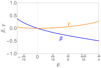
Figure 4: Wavefunction parameters $\beta$ and $\gamma$ [see Eq. (29)] determined in CMFT as a function of the exchange parameter $\theta$, in the region of parameter space corresponding to the QSI₀ and QSI_π phases. These determine the overlap and Hamiltonian matrix elements between different CMFT ground states and function as the small parameters for the expansion of the cVAR variational energy.

To evaluate $O_{\{\sigma^{\prime}\}\{\sigma\}}$ and $X_{\{\sigma^{\prime}\}\{\sigma\}}$ we need to calculate the overlaps and Hamiltonian matrix elements between the single tetrahedron wavefunctions. These are

$$\langle+-+-|++--\rangle=\beta\left(\sqrt{1-\beta^{2}-\gamma^{2}}+\gamma+\frac{\beta}{2}\right)$$ (30)

$$\langle--++|++--\rangle=\beta^{2}+2\gamma\sqrt{1-\beta^{2}-\gamma^{2}}$$ (31)

$$\langle+-+-|S^{z}_{0}|++--\rangle=\frac{\beta}{2}\left(\sqrt{1-\beta^{2}-\gamma^{2}}-\gamma\right)$$ (32)

$$\langle-+-+|S^{z}_{0}|++--\rangle=\langle--++|S^{z}_{0}|++--\rangle=0$$ (33)

$$\langle-+-+|S^{x}_{0}|++--\rangle=\langle--++|S^{x}_{0}|++--\rangle=0$$ (34)

(35)

$$\langle+-+-|\mathcal{H}_{\sf XXZ}^{(A)}|++--\rangle=-\frac{J}{4}\cos(\theta)\beta\left(\beta+2(\gamma+\sqrt{1-\beta^{2}-\gamma^{2}})\right)+J\sin(\theta)\left(\frac{1}{2}+(\beta+\gamma)(\beta+\sqrt{1-\beta^{2}-\gamma^{2}})\right)$$

(36)

$$\langle--++|\mathcal{H}_{\sf XXZ}^{(A)}|++--\rangle=-J\cos(\theta)\left(\frac{\beta^{2}}{2}+\gamma\sqrt{1-\beta^{2}-\gamma^{2}}\right)+J\sin(\theta)\beta\left(\beta+2(\gamma+\sqrt{1-\beta^{2}-\gamma^{2}})\right)$$ (37)

where $\mathcal{H}_{\sf XXZ}^{(A)}$ is the Hamiltonian on the ‘$A$’ tetrahedra. All the other relevant overlaps and matrix elements can be generated from Eqs. (30)-(37) using symmetries of the problem.

Both $\beta$ and $\gamma$ are significantly smaller than 1 over the whole regime where the optimal CMFT state is of the form of Eq. (22) [see Fig. 4]. Using this fact we can expand Eqs. (30)-(37) to linear order in $\beta,\gamma$ and obtain

$$\langle+-+-|++--\rangle\approx\beta$$ (38)

$$\langle--++|++--\rangle\approx 2\gamma$$ (39)

$$\langle+-+-|S^{z}_{0}|++--\rangle\approx\frac{\beta}{2}$$ (40)

$$\langle+-+-|\mathcal{H}_{\sf XXZ}^{(A)}|++--\rangle\approx-\frac{J}{2}\cos(\theta)\beta+J\sin(\theta)\left(\frac{1}{2}+(\beta+\gamma)\right)$$

(41)

$$\langle--++|\mathcal{H}_{\sf XXZ}^{(A)}|++--\rangle\approx-J\cos(\theta)\gamma+2J\sin(\theta)\beta$$ (42)

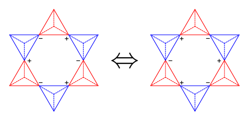
Figure 5: CMFT wavefunctions related by flipping the sign variables $\sigma_{i}=\pm 1$ around a single hexagonal plaquette provided the leading terms in the expansions of $X_{\{\sigma^{\prime}\},\{\sigma\}}$ and $O_{\{\sigma^{\prime}\},\{\sigma\}}$ [Eqs. (26), (27), (43), (44)].

Using these results and Eq. (13) we can find the leading terms in $\beta$ and $\gamma$ in the numerator and denominator of Eq. (28). The leading term in the sums in both numerator and denominator comes from pairs of configurations $\{\sigma\}$ and $\{\sigma^{\prime}\}$ which are related by reversing the sign factors $\sigma_{i}$ on six sites around a single hexagonal plaquette [Fig. 5]. For two such configurations we have

$$X_{\{\sigma^{\prime}\}\{\sigma\}}=\frac{3}{2}J\sin(\theta)\beta^{2}+\mathcal{O}(\beta^{3})$$ (43)

$$O_{\{\sigma^{\prime}\}\{\sigma\}}=\beta^{3}+\mathcal{O}(\beta^{4}).$$ (44)

Using this to expand Eq. (28) up to order $\beta^{2}$, gives a new equation for the variational energy

$$E_{\sf var}^{\sf cVAR}\approx E_{\sf var}^{\sf CMFT}+\sum_{\{\sigma\}\neq\{\sigma^{\prime}\}}M_{\{\sigma^{\prime}\}\{\sigma\}})a_{\{\sigma^{\prime}\}}^{\ast}a_{\{\sigma\}}^{\phantom{\ast}}$$ (45)

where

$$M_{\{\sigma^{\prime}\}\{\sigma\}}=\frac{3}{2}J\sin(\theta)\beta^{2}$$ (46)

for two configurations related by flipping a single hexagonal plaquette and zero otherwise.

We now face the problem of finding the set of coefficients $a_{\{{\bf h}\}}$ which will optimize the expanded variational energy Eq. (45), as a function of $\theta$. Fortunately, the solution to this problem is already known.

Optimizing the variational energy in Eq. (45) is equivalent to solving the ring exchange problem studied by Quantum Monte Carlo in Ref. Shannon et al. (2012). The results tell us that when $M_{\{\sigma^{\prime}\}\{\sigma\}}<0$ the optimum wavefunction is the 0-flux $U(1)$ quantum spin liquid which we refer to as QSI₀. Since $M_{\{\sigma^{\prime}\}\{\sigma\}}$ has the same sign as $\sin(\theta)$, this leads us to assign the region $-0.26<\theta<0$ to the QSI₀ phase.

For $\theta>0\implies M_{\{\sigma^{\prime}\}\{\sigma\}}>0$ we have the same problem but now with a positive tunnelling matrix element. Using a gauge transformation described in Refs. Hermele et al. (2004); Lee et al. (2012) one can relate this case back to the case with $M_{\{\sigma^{\prime}\}\{\sigma\}}<0$, and find that the ground state is also a quantum spin liquid but now of the $\pi$-flux variety ( QSI_π). We therefore assign the region $0<\theta<\frac{\pi}{4}$ to the QSI_π phase.

We therefore identify the phase boundary between 0-flux and $\pi$-flux QSLs at $\theta=0$, which is in agreement with the known result from perturbation theory Hermele et al. (2004); Lee et al. (2012).

II.2 cVAR for QSN_⟂

Having established the general method, and applied it to distinguish between the 0-flux and $\pi$-flux QSLs in the region with spin-ice-like CMFT ground states, we now demonstrate its application for the region of strong frustrated transverse exchange $\frac{\pi}{4}<\theta\lesssim 1.93$.

In this region, the optimal CMFT solutions correspond to field configurations of the form

$${\bf h}_{i}=\sigma_{i}h\hat{{\bf x}},\quad\sigma_{i}=\pm 1$$ (47)

and those related to Eq. (47) by global symmetry transformations. The choice of a global axis within the $xy$ plane for ${\bf h}_{i}$ indicates the spontaneous breaking of $U(1)$ spin rotation symmetry. The sign variables $\sigma_{i}=\pm 1$ can take on any one of an extensively large number of configurations obeying the constraint Eq. (23) on every tetrahedron of the lattice.

We proceed with the cVAR method in precisely the same way as above: by writing down a new wavefunction which is a superposition of CMFT solutions [Eq. (19)] and seeking to optimize its variational energy [Eq. (21)].

We consider a superposition of CMFT solutions

$$|\psi^{\sf CMFT}(\{\sigma\})\rangle=|\psi^{\sf CMFT}(\{h\sigma\hat{\bf x}\})\rangle$$ (48)

with a fixed global axis of collinearity (in this case $\hat{{\bf x}}$). Pairs of CMFT wavefunctions with different global axes of collinearity have vanishing overlaps and Hamiltonian matrix elements between them in the thermodynamic limit, so superposing states with different collinearity axes would not improve the variational energy.

To write down the single tetrahedron wavefunctions, from which the CMFT wavefunctions are formed via Eq. (13), it is convenient to use the basis of eigenstates of ${\sf S}^{x}_{i}$ which we write as $|\rightarrow\rangle,|\leftarrow\rangle$. As before, there are six possible single tetrahedron wavefunctions, indexed by 6 possible arrangements of signs $\sigma_{i}$, constrained by Eq. (23).

$$|++--\rangle=\sqrt{1-\mu^{2}-\nu^{2}-\rho^{2}}|\rightarrow\rightarrow\leftarrow\leftarrow\rangle+\frac{\mu}{2}\bigg{(}|\rightarrow\leftarrow\rightarrow\leftarrow\rangle+|\rightarrow\leftarrow\leftarrow\rightarrow\rangle+|\leftarrow\rightarrow\rightarrow\leftarrow\rangle+|\leftarrow\rightarrow\leftarrow\rightarrow\rangle\bigg{)}+\nu|\leftarrow\leftarrow\rightarrow\rightarrow\rangle$$

$$\qquad\qquad\qquad+\frac{\rho}{\sqrt{2}}(|\leftarrow\leftarrow\leftarrow\leftarrow\rangle+|\rightarrow\rightarrow\rightarrow\rightarrow\rightarrow)$$

$$|+-+-\rangle=\sqrt{1-\mu^{2}-\nu^{2}-\rho^{2}}|\rightarrow\leftarrow\rightarrow\leftarrow\rangle+\frac{\mu}{2}\bigg{(}|\rightarrow\rightarrow\leftarrow\leftarrow\rangle+|\rightarrow\leftarrow\leftarrow\rightarrow\rangle+|\leftarrow\rightarrow\rightarrow\leftarrow\rangle+|\leftarrow\leftarrow\rightarrow\rightarrow\rangle\bigg{)}+\nu|\leftarrow\rightarrow\leftarrow\rightarrow\rangle$$

$$\qquad\qquad\qquad+\frac{\rho}{\sqrt{2}}(|\leftarrow\leftarrow\leftarrow\leftarrow\rangle+|\rightarrow\rightarrow\rightarrow\rightarrow\rightarrow)$$

$$|+--+\rangle=\sqrt{1-\mu^{2}-\nu^{2}-\rho^{2}}|\rightarrow\leftarrow\leftarrow\rightarrow\rangle+\frac{\mu}{2}\bigg{(}|\rightarrow\rightarrow\leftarrow\leftarrow\rangle+|\rightarrow\leftarrow\rightarrow\leftarrow\rangle+|\leftarrow\rightarrow\leftarrow\rightarrow\rangle+|\leftarrow\leftarrow\rightarrow\rightarrow\rangle\bigg{)}+\nu|\leftarrow\rightarrow\rightarrow\leftarrow\rangle$$

$$\qquad\qquad\qquad+\frac{\rho}{\sqrt{2}}(|\leftarrow\leftarrow\leftarrow\leftarrow\rangle+|\rightarrow\rightarrow\rightarrow\rightarrow\rightarrow)$$

$$|-++-\rangle=\sqrt{1-\mu^{2}-\nu^{2}-\rho^{2}}|\leftarrow\rightarrow\rightarrow\leftarrow\rangle+\frac{\mu}{2}\bigg{(}|\rightarrow\rightarrow\leftarrow\leftarrow\rangle+|\rightarrow\leftarrow\rightarrow\leftarrow\rangle+|\leftarrow\rightarrow\leftarrow\rightarrow\rangle+|\leftarrow\leftarrow\rightarrow\rightarrow\rangle\bigg{)}+\nu|\rightarrow\leftarrow\leftarrow\rightarrow\rangle$$

$$\qquad\qquad\qquad+\frac{\rho}{\sqrt{2}}(|\leftarrow\leftarrow\leftarrow\leftarrow\rangle+|\rightarrow\rightarrow\rightarrow\rightarrow\rightarrow)$$

$$|-+-+\rangle=\sqrt{1-\mu^{2}-\nu^{2}-\rho^{2}}|\leftarrow\rightarrow\leftarrow\rightarrow\rangle+\frac{\mu}{2}\bigg{(}|\rightarrow\rightarrow\leftarrow\leftarrow\rangle+|\rightarrow\leftarrow\leftarrow\rightarrow\rangle+|\leftarrow\rightarrow\rightarrow\leftarrow\rangle+|\leftarrow\leftarrow\rightarrow\rightarrow\rangle\bigg{)}+\nu|\rightarrow\leftarrow\rightarrow\leftarrow\rangle$$

$$\qquad\qquad\qquad+\frac{\rho}{\sqrt{2}}(|\leftarrow\leftarrow\leftarrow\leftarrow\rangle+|\rightarrow\rightarrow\rightarrow\rightarrow\rightarrow)$$

$$|--++\rangle=\sqrt{1-\mu^{2}-\nu^{2}-\rho^{2}}|\leftarrow\leftarrow\rightarrow\rightarrow\rangle+\frac{\mu}{2}\bigg{(}|\rightarrow\leftarrow\rightarrow\leftarrow\rangle+|\rightarrow\leftarrow\leftarrow\rightarrow\rangle+|\leftarrow\rightarrow\rightarrow\leftarrow\rangle+|\leftarrow\rightarrow\leftarrow\rightarrow\rangle\bigg{)}+\nu|\rightarrow\rightarrow\leftarrow\leftarrow\rangle$$

$$\qquad\qquad\qquad+\frac{\rho}{\sqrt{2}}(|\leftarrow\leftarrow\leftarrow\leftarrow\rangle+|\rightarrow\rightarrow\rightarrow\rightarrow\rightarrow)$$ (49)

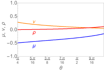
Figure 6: Wavefunction parameters $\mu$, $\nu$ and $\rho$ [see Eq. (49)] determined in CMFT as a function of the exchange parameter $\theta$, in the region of parameter space corresponding to the nematic QSL phase. These determine the overlap and Hamiltonian matrix elements between different CMFT ground states and function as the small parameters for the expansion of the cVAR variational energy.

The wavefunction parameters $\mu,\nu,\rho$ are plotted as a function of $\theta$ in Fig. 6. These remain small throughout the relevant region of parameter space and we use them as small parameters in an expansion of the variational energy Eq. 28.

Up to linear order in $\mu,\nu,\rho$:

$$\langle+-+-|++--\rangle\approx\mu$$ (50)

$$\langle--++|++--\rangle\approx 2\nu$$ (51)

$$\langle+-+-|S^{x}_{0}|++--\rangle\approx\frac{\mu}{2}$$ (52)

$$\langle+-+-|\mathcal{H}_{\sf XXZ}^{(A)}|++--\rangle\approx\frac{J}{4}(\sin(\theta)+\cos(\theta))+\frac{J}{2}(\mu+\nu+\sqrt{2}\rho)\cos(\theta)+\frac{J}{2}(\nu-\sqrt{2}\rho)\sin(\theta)+$$

(53)

$$\langle--++|\mathcal{H}_{\sf XXZ}^{(A)}|++--\rangle\approx J\left(\mu\cos(\theta)+\frac{\rho\cos(\theta)}{\sqrt{2}}+\mu\sin(\theta)-\nu\sin(\theta)-\frac{\rho\sin(\theta)}{\sqrt{2}}\right).$$ (54)

From this we can calculate the leading terms in $\mu,\nu,\rho$ in both numerator and denominator of Eq. 28. Once again the leading terms come from pairs of configuratons $\{\sigma\}$ and $\{\sigma^{\prime}\}$ related by reversing the sign factors $\sigma_{i}$ on six sites around a single hexagonal plaquette [Fig. (5)]. We have

$${X}_{\{\sigma^{\prime}\}\{\sigma\}}\approx\frac{3J}{4}(\cos(\theta)+\sin(\theta))\mu^{2}+\mathcal{O}(\mu^{3})$$ (55)

$${O}_{\{\sigma^{\prime}\}\{\sigma\}}\approx\mu^{3}+\mathcal{O}(\mu^{4})$$ (56)

Using this to expand Eq. (28) up to order $\mu^{2}$, gives

$$E_{\sf var}^{\sf cVAR}\approx E_{\sf var}^{\sf CMFT}+\sum_{\{\sigma\}\neq\{\sigma^{\prime}\}}M_{\{\sigma^{\prime}\}\{\sigma\}}a_{\{\sigma^{\prime}\}}^{\ast}a_{\{\sigma\}}^{\phantom{\ast}}$$ (57)

where now

$$M_{\{\sigma^{\prime}\}\{\sigma\}}=\frac{3J}{4}(\cos(\theta)+\sin(\theta))\mu^{2}+\mathcal{O}(\mu^{3})$$ (58)

for two configurations related by flipping a single hexagonal plaquette and zero otherwise.

Once again, optimizing such a variational energy is equivalent to solving the ring–exchange problem studied by Quantum Monte Carlo in Ref. Shannon et al. (2012). It follows that the cVAR solution in this case is also a U(1) QSL, but one with finite spin–nematic order, since its wavefunction is a superposition of states with the same value of the nematic order parameter. We note that the value of the effective ring-tunnelling is positive throughout the relevant region of parameter space, such that the nematic QSL should have the same $U(1)$ flux pattern, and fractionalization of translational symmetry, as QSI_π. It differs from that phase, however, by the presence of nematic order. This can be seen by calculating the nematic order parameter [Eq. (7) of main text] within the cVAR wavefunction, giving

$$|\mathcal{Q}_{\perp}|=\frac{1}{6}\left[1-\left(\frac{\rho}{\sqrt{2}}-\mu\right)+\mathcal{O}(\mu^{2})\right]\;,$$ (59)

where the parameters $\rho$ and $\mu$ take on the values shown in Fig. 6.

III Series expansion methods

III.1 High Temperature Expansions

High temperature series expansion is a well known method for calculating properties of statistical models Oitmaa et al. (2006). Finite temperature properties (for example $A$) of the models, in the thermodynamic limit, are expanded in powers of the inverse temperature $\beta$.

$$A(\beta)=a_{0}+a_{1}\beta+a_{2}\beta^{2}+a_{3}\beta^{3}+\ldots$$ (60)

The coefficients $a_{n}$ are calculated up to some maximum order $n=N$ and these are used to numerically evaluate the property $A(\beta)$ at different temperatures. For lattice statistical models, with short-range interactions, these expansion converge absolutely at sufficiently high temperatures and provide accurate estimates of the properties. At lower temperatures, outside the radius of convergence of the power series, one can use series extrapolation methods (such as Pade and d-log Pade approximants) to enhance the range of numerical convergence.

One efficient way to generate the series coefficients is by the Linked Cluster method. In the Linked Cluster formalism, an extensive property $P$ for a large translationally invariant lattice ${\mathcal{L}}$ with $N$-sites is expressed as a sum over all distinct linked clusters $c$ as

$${P(\mathcal{L})\over N}=\sum_{c}L(c)\ W(c).$$ (61)

Here $L(c)$, called the lattice constant, is the number of embeddings of the cluster $c$, per site, in the lattice $\mathcal{L}$. This is a geometrical property that only depends on the lattice under consideration and not on the statistical model. The quantity $W(c)$ is called the weight of the cluster. It is defined by the recursive relation

$$W(c)=P(c)-\sum_{c^{\prime}}W(c^{\prime}).$$ (62)

Here the sum is over all proper subclusters $c^{\prime}$ of the cluster $c$. The quantity $P(c)$ is the property for the finite cluster. Thus $W(c)$ is entirely defined by the finite cluster $c$, and does not depend on the larger lattice. If one can calculate the series expansions for small clusters, then starting with the smallest cluster, Eq. (62) can be used to calculate the series expansions for the weights of the clusters. One can prove that the weight of a cluster with $N$ bonds is of order $\beta^{N}$. Thus, once the weights of all clusters up to size $N$ have been calculated, the series expansion for the infinite cluster to order $N$ follows.

We have used the HTE method to calculate the logarithm of the partition function $\ln{Z}$ from which thermodynamic properties such as entropy, specific heat and free energy follow. In addition, we can apply a field associated with some order-parameter and by calculating the free-energy to second order in that field we can calculate the static susceptibilities associated with that order. Here, we have calculated static susceptibilities associated with various magnetic order parameters as well as for the nematic order parameter.

III.2 Numerical Linked Cluster Expansions

Numerical Linked Cluster (NLC) method is a systematic way to calculate thermodynamic and ground state properties of lattice statistical models in the thermodynamic limit Rigol et al. (2006). The method uses the graphical basis of series expansions (such as high temperature expansions) to express model properties as a sum of suitably defined weights over all linked clusters. Rather than obtain weights $W(c)$ as a power series in some variable, NLC uses exact diagonalization to calculate them numerically. The calculations are carried out up to some maximum cluster size, $n$, also called the order of the calculation, providing an estimate for the property ($P_{n}$) in each order.

The method has the advantage of being non-perturbative, of incorporating exact information at short distances, and building the thermodynamic limit into the formalism. For some problems, it has proven to be more accurate than high temperature series expansions.

For the NLC method, it is often useful to consider clusters consisting only of complete units of an extended size. For example, here, on the pyrochlore lattice consisting of corner-sharing tetrahedra, it proves useful to only consider clusters that consist of complete tetrahedra Applegate et al. (2012); Hayre et al. (2013); Oitmaa et al. (2013); Jaubert et al. (2015). This avoids strong oscillations caused by clusters with free ends. For the classical spin-ice problem, the first order NLC in terms of tetrahedra, is equivalent to the well-known Pauling approximation and is already very accurate down to $T=0$ Singh and Oitmaa (2012). This also greatly simplifies the problem of graph counting as there are very few clusters of complete tetrahedra in each order.

The NLC calculations are limited by one’s ability to exactly diagonalize finite clusters. For a general model of quantum spin-ice a 4th order NLC calculation, involving sum over weights for clusters up to 4 tetrahedra were done Applegate et al. (2012); Hayre et al. (2013); Oitmaa et al. (2013); Jaubert et al. (2015). The maximum number of sites in these clusters was 13. Here, for the XXZ model of interest, $S_{z}$ is a good quantum number. This allows one to go to go one further order and calculate NLC to 5th order. The largest cluster needed for such a calculation has 16 sites.

Since exact diagonalization of finite clusters leads to energy-levels and wave-functions, the method is most suitable for calculating thermodynamic properties such as specific heat and entropy and various equal-time thermal correlation functions. Frequency dependent properties do not usually have a convergent NLC expansion at any temperature. Static linear response functions can be calculated but require numerical differentiation of the free energy with respect to an applied field. This reduces the accuracy of the calculation. Here we have used NLC to calculate thermodynamic properties and the thermal expectation values of the squares of various order parameters.

When correlations in the system are short-ranged, $P_{n}$ converges rapidly with $n$ and provides a highly accurate numerical value of the property $P$ in the thermodynamic limit. When correlation lengths begin to exceed the sizes of the clusters studied, one can use sequence extrapolation methods to estimate the limit of the sequence $\{P_{n}\}$. We have found it useful to consider Euler transformations starting with third order. This ameliorates some of the strong oscillations in $\{P_{n}\}$ with $n$ and improves the apparent convergence down to slightly lower temperatures.

References

- Gardner et al. (2010) Jason S. Gardner, Michel J. P. Gingras, and John E. Greedan, “Magnetic pyrochlore oxides,” Rev. Mod. Phys. 82, 53–107 (2010).
- Hallas et al. (2018) A. M. Hallas, J. Gaudet, and B. D. Gaulin, “Experimental Insights into Ground State Selection of Quantum XY Pyrochlores,” Annu. Rev. Condens. Matter Phys. 9, 105 (2018).
- Bramwell and Gingras (2001) S. T. Bramwell and M. J. P. Gingras, “Spin Ice State in Frustrated Magnetic Pyrochlore Materials,” Science 294 (2001).
- Castelnovo et al. (2012) C. Castelnovo, R. Moessner, and S.L. Sondhi, “Spin Ice, Fractionalization, and Topological Order,” Annu. Rev. Condens. Matter Phys. 3, 35 (2012).
- Castelnovo et al. (2008) C. Castelnovo, R. Moessner, and S. L. Sondhi, “Magnetic monopoles in spin ice,” Nature 451, 42–45 (2008).
- Balents (2010) L. Balents, “Spin liquids in frustrated magnets,” Nature (London) 464, 199 (2010).
- Savary and Balents (2017a) L. Savary and L. Balents, “Quantum spin liquids: a review,” Rep. Prog. Phys. 80, 016502 (2017a).
- Zhou et al. (2017) Y. Zhou, K. Kanoda, and T. K. Ng, “Quantum spin liquid states,” Rev. Mod. Phys. 89, 025003 (2017).
- Norman (2016) M. R. Norman, “Colloquium: Herbertsmithite and the search for the quantum spin liquid,” Rev. Mod. Phys. 88, 041002 (2016).
- Hermele et al. (2004) M. Hermele, M. P. A. Fisher, and L. Balents, “Pyrochlore photons: The U(1) spin liquid in a S= three-dimensional frustrated magnet,” Phys. Rev. B 69, 064404 (2004).
- Banerjee et al. (2008) A. Banerjee, S. V. Isakov, K. Damle, and Y. B. Kim, “Unusual Liquid State of Hard-Core Bosons on the Pyrochlore Lattice,” Phys. Rev. Lett. 100, 047208 (2008).
- Shannon et al. (2012) N. Shannon, O. Sikora, F. Pollmann, K. Penc, and P. Fulde, “Quantum Ice: A Quantum Monte Carlo Study,” Phys. Rev. Lett. 108, 067204 (2012).
- Benton et al. (2012) O. Benton, O. Sikora, and N. Shannon, “Seeing the light: Experimental signatures of emergent electromagnetism in a quantum spin ice,” Phys. Rev. B 86, 075154 (2012).
- Kato and Onoda (2015) Y. Kato and S. Onoda, “Numerical Evidence of Quantum Melting of Spin Ice: Quantum-to-Classical Crossover,” Phys. Rev. Lett. 115, 077202 (2015).
- (15) C.-J. Huang, Y. Deng, Y. Wan, and Z. Y. Meng, “Dynamics of topological excitations in a model quantum spin ice,” arXiv:1707.00099 .
- Ross et al. (2011) K. A. Ross, L. Savary, B. D. Gaulin, and L. Balents, “Quantum Excitations in Quantum Spin Ice,” Phys. Rev. X 1, 021002 (2011).
- Kimura et al. (2013) K. Kimura, S. Nakatsuji, J-J. Wen, C. Broholm, M. B. Stone, E. Nishibori, and H. Sawa, “Quantum fluctuations in spin-ice-like ,” Nat. Commun. 4 (2013).
- Petit et al. (2016) S. Petit, E. Lhotel, S. Guitteny, O. Florea, J. Robert, P. Bonville, I. Mirebeau, J. Ollivier, H. Mutka, E. Ressouche, C. Decorse, M. Ciomaga Hatnean, and G. Balakrishnan, “Antiferroquadrupolar correlations in the quantum spin ice candidate ,” Phys. Rev. B 94, 165153 (2016).
- Wen et al. (2017) J.-J. Wen, S. M. Koohpayeh, K. A. Ross, B. A. Trump, T. M. McQueen, K. Kimura, S. Nakatsuji, Y. Qiu, D. M. Pajerowski, J. R. D. Copley, and C. L. Broholm, “Disordered Route to the Coulomb Quantum Spin Liquid: Random Transverse Fields on Spin Ice in ,” Phys. Rev. Lett. 118, 107206 (2017).
- Martin et al. (2017) N. Martin, P. Bonville, E. Lhotel, S. Guitteny, A. Wildes, C. Decorse, M. Ciomaga Hatnean, G. Balakrishnan, I. Mirebeau, and S. Petit, “Disorder and quantum spin ice,” Phys. Rev. X 7, 041028 (2017).
- (21) R. Sibille, N. Gauthier, H. Yan, M. C. Hatnean, J. Ollivier, B. Winn, G. Balakrishnan, M. Kenzelmann, N. Shannon, and T. Fennell, “Experimental signatures of emergent quantum electrodynamics in a quantum spin ice,” arXiv:1706.03604 .
- Onoda and Tanaka (2011) S. Onoda and Y. Tanaka, “Quantum fluctuations in the effective pseudospin- model for magnetic pyrochlore oxides,” Phys. Rev. B 83, 094411 (2011).
- Benton et al. (2016) O. Benton, L. D. C. Jaubert, H. Yan, and N. Shannon, “A spin-liquid with pinch-line singularities on the pyrochlore lattice,” Nat. Commun. 7, 11572 (2016).
- Yan et al. (2017) H. Yan, O. Benton, L. Jaubert, and N. Shannon, “Theory of multiple-phase competition in pyrochlore magnets with anisotropic exchange with application to , and ,” Phys. Rev. B 95, 094422 (2017).
- Taillefumier et al. (2017) Mathieu Taillefumier, Owen Benton, Han Yan, L. D. C. Jaubert, and Nic Shannon, “Competing spin liquids and hidden spin-nematic order in spin ice with frustrated transverse exchange,” Phys. Rev. X 7, 041057 (2017).
- Lee et al. (2012) S. B. Lee, S. Onoda, and L. Balents, “Generic quantum spin ice,” Phys. Rev. B 86, 104412 (2012).
- Chen (2017a) G. Chen, “Spectral periodicity of the spinon continuum in quantum spin ice,” Phys. Rev. B 96, 085136 (2017a).
- Grover et al. (2010) Tarun Grover, N. Trivedi, T. Senthil, and Patrick A. Lee, “Weak mott insulators on the triangular lattice: Possibility of a gapless nematic quantum spin liquid,” Phys. Rev. B 81, 245121 (2010).
- Molavian et al. (2007) H. R. Molavian, M. J. P. Gingras, and B. Canals, “Dynamically Induced Frustration as a Route to a Quantum Spin Ice State in via Virtual Crystal Field Excitations and Quantum Many-Body Effects,” Phys. Rev. Lett. 98, 157204 (2007).
- Onoda and Tanaka (2010) S. Onoda and Y. Tanaka, “Quantum Melting of Spin Ice: Emergent Cooperative Quadrupole and Chirality,” Phys. Rev. Lett. 105, 047201 (2010).
- Savary and Balents (2012) L. Savary and L. Balents, “Coulombic Quantum Liquids in Spin- Pyrochlores,” Phys. Rev. Lett. 108, 037202 (2012).
- Hao et al. (2014) Z. Hao, A. G. R. Day, and M. J. P. Gingras, “Bosonic many-body theory of quantum spin ice,” Phys. Rev. B 90, 214430 (2014).
- McClarty et al. (2015) P. A. McClarty, O. Sikora, R. Moessner, K. Penc, F. Pollmann, and N. Shannon, “Chain-based order and quantum spin liquids in dipolar spin ice,” Phys. Rev. B 92, 094418 (2015).
- Gingras and McClarty (2014) M. J. P. Gingras and P. A. McClarty, “Quantum spin ice: a search for gapless quantum spin liquids in pyrochlore magnets,” Rep. Prog. Phys. 77, 056501 (2014).
- Chen (2016) G. Chen, “ “Magnetic monopole” condensation of the pyrochlore ice U(1) quantum spin liquid: Application to and ,” Phys. Rev. B 94, 205107 (2016).
- Shannon (2017) N. Shannon, “Spin Ice,” (Springer, 2017) Chap. “Quantum Monte Carlo simulations of quantum spin ice”.
- Savary and Balents (2017b) L. Savary and L. Balents, “Disorder-Induced Quantum Spin Liquid in Spin Ice Pyrochlores,” Phys. Rev. Lett. 118, 087203 (2017b).
- Chen (2017b) Gang Chen, “Dirac’s “magnetic monopoles” in pyrochlore ice spin liquids: Spectrum and classification,” Phys. Rev. B 96, 195127 (2017b).
- García-Adeva and Huber (2000) A. J. García-Adeva and D. L. Huber, “Quantum Tetrahedral Mean Field Theory of the Magnetic Susceptibility for the Pyrochlore Lattice,” Phys. Rev. Lett. 85, 4598–4601 (2000).
- García-Adeva and Huber (2001) A. J. García-Adeva and D. L. Huber, “Quantum tetrahedral mean-field theory of the pyrochlore lattice,” Can. J. Phys. 79, 1359–1364 (2001).
- Shannon (2002) Nic Shannon, “Mixed valence on a pyrochlore lattice – liv2o4 as a geometrically frustrated magnet,” Eur. Phys. J. B 27, 527 (2002).
- Yamamoto et al. (2014) D. Yamamoto, G. Marmorini, and I. Danshita, “Quantum Phase Diagram of the Triangular-Lattice Model in a Magnetic Field,” Phys. Rev. Lett. 112, 127203 (2014).
- Javanparast et al. (2015) B. Javanparast, A. G. R. Day, Z. Hao, and M. J. P. Gingras, “Order-by-disorder near criticality in pyrochlore magnets,” Phys. Rev. B 91, 174424 (2015).
- Yamamoto et al. (2015) Daisuke Yamamoto, Giacomo Marmorini, and Ippei Danshita, “Microscopic model calculations for the magnetization process of layered triangular-lattice quantum antiferromagnets,” Phys. Rev. Lett. 114, 027201 (2015).
- Harris et al. (1991) A. B. Harris, A. J. Berlinsky, and C. Bruder, “Ordering by quantum fluctuations in a strongly frustrated Heisenberg antiferromagnet,” J. App. Phys. 69, 5200–5202 (1991).
- Berg et al. (2003) E. Berg, E. Altman, and A. Auerbach, “Singlet Excitations in Pyrochlore: A Study of Quantum Frustration,” Phys. Rev. Lett. 90, 147204 (2003).
- Tsunetsugu (2001a) H. Tsunetsugu, “Antiferromagnetic Quantum Spins on the Pyrochlore Lattice,” J. Phys. Soc. Jpn 70, 640–643 (2001a).
- Tsunetsugu (2001b) H. Tsunetsugu, “Spin-singlet order in a pyrochlore antiferromagnet,” Phys. Rev. B 65, 024415 (2001b).
- Moessner et al. (2006) R. Moessner, S. L. Sondhi, and M. O. Goerbig, “Quantum dimer models and effective Hamiltonians on the pyrochlore lattice,” Phys. Rev. B 73, 094430 (2006).
- Canals and Lacroix (1998) B. Canals and C. Lacroix, “Pyrochlore Antiferromagnet: A Three-Dimensional Quantum Spin Liquid,” Phys. Rev. Lett. 80, 2933 (1998).
- Canals and Lacroix (2000) B. Canals and C. Lacroix, “Quantum spin liquid: The Heisenberg antiferromagnet on the three-dimensional pyrochlore lattice,” Phys. Rev. B 61, 1149–1159 (2000).
- Kim and Han (2008) J. H. Kim and J. H. Han, “Chiral spin states in the pyrochlore Heisenberg magnet: Fermionic mean-field theory and variational Monte Carlo calculations,” Phys. Rev. B 78, 180410 (2008).
- Burnell et al. (2009) F. J. Burnell, S. Chakravarty, and S. L. Sondhi, “Monopole flux state on the pyrochlore lattice,” Phys. Rev. B 79, 144432 (2009).
- Shannon et al. (2006) N. Shannon, T. Momoi, and P. Sindzingre, “Nematic Order in Square Lattice Frustrated Ferromagnets,” Phys. Rev. Lett. 96, 027213 (2006).
- Oitmaa et al. (2006) J. Oitmaa, C. Hamer, and W. Zheng, Series Expansion Methods for Strongly Interacting Lattice Models (Cambridge University Press, Cambridge, England, 2006).
- Oitmaa et al. (2013) J. Oitmaa, R. R. P. Singh, B. Javanparast, A. G. R. Day, B. V. Bagheri, and M. J. P. Gingras, “Phase transition and thermal order-by-disorder in the pyrochlore antiferromagnet Er2Ti2O7: A high-temperature series expansion study,” Phys. Rev. B 88, 220404 (2013).
- Jaubert et al. (2015) L. D. C. Jaubert, O. Benton, J. G. Rau, J. Oitmaa, R. R. P. Singh, N. Shannon, and M. J. P. Gingras, “Are Multiphase Competition and Order by Disorder the Keys to Understanding ?” Phys. Rev. Lett. 115, 267208 (2015).
- Applegate et al. (2012) R. Applegate, N. R. Hayre, R. R. P. Singh, T. Lin, A. G. R. Day, and M. J. P. Gingras, “Vindication of as a Model Exchange Quantum Spin Ice,” Phys. Rev. Lett. 109, 097205 (2012).
- Tang et al. (2013) B. Tang, E. Khatami, and M. Rigol, “A short introduction to numerical linked-cluster expansions,” Comp. Phys. Commun. 184, 557 – 564 (2013).
- Huang et al. (2016) Y. Huang, K. Chen, Y. Deng, N. Prokof’ev, and B. Svistunov, “Spin-Ice State of the Quantum Heisenberg Antiferromagnet on the Pyrochlore Lattice,” Phys. Rev. Lett. 116, 177203 (2016).
- Smerald and Shannon (2013) A. Smerald and N. Shannon, “Theory of spin excitations in a quantum spin-nematic state,” Phys. Rev. B 88, 184430 (2013).
- Anand et al. (2016) V. K. Anand, L. Opherden, J. Xu, D. T. Adroja, A. T. M. N. Islam, T. Herrmannsdörfer, J. Hornung, R. Schönemann, M. Uhlarz, H. C. Walker, N. Casati, and B. Lake, “Physical properties of the candidate quantum spin-ice system ,” Phys. Rev. B 94, 144415 (2016).
- Yaouanc et al. (2011) A. Yaouanc, P. Dalmas de Réotier, C. Marin, and V. Glazkov, “Single-crystal versus polycrystalline samples of magnetically frustrated Yb2Ti2O7: Specific heat results,” Phys. Rev. B 84, 172408 (2011).
- Ross et al. (2012) K. A. Ross, Th. Proffen, H. A. Dabkowska, J. A. Quilliam, L. R. Yaraskavitch, J. B. Kycia, and B. D. Gaulin, “Lightly stuffed pyrochlore structure of single-crystalline grown by the optical floating zone technique,” Phys. Rev. B 86, 174424 (2012).
- Taniguchi et al. (2013) T. Taniguchi, H. Kadowaki, H. Takatsu, B. Fåk, J. Ollivier, T. Yamazaki, T. J. Sato, H. Yoshizawa, Y. Shimura, T. Sakakibara, T. Hong, K. Goto, L. R. Yaraskavitch, and J. B. Kycia, “Long-range order and spin-liquid states of polycrystalline ,” Phys. Rev. B 87, 060408 (2013).
- Benton (2017) O. Benton, “From quantum spin liquid to paramagnetic ground states in disordered non-Kramers pyrochlores,” arXiv:1706.09238 (2017).
- Sibille et al. (2015) R. Sibille, E. Lhotel, V. Pomjakushin, C. Baines, T. Fennell, and M. Kenzelmann, “Candidate Quantum Spin Liquid in the Pyrochlore Stannate ,” Phys. Rev. Lett. 115, 097202 (2015).
- Wiebe and Hallas (2015) C. R. Wiebe and A. M. Hallas, “Frustration under pressure: Exotic magnetism in new pyrochlore oxides,” APL Materials 3, 041519 (2015).
- Rigol et al. (2006) Marcos Rigol, Tyler Bryant, and Rajiv R. P. Singh, “Numerical linked-cluster approach to quantum lattice models,” Phys. Rev. Lett. 97, 187202 (2006).
- Hayre et al. (2013) N. R. Hayre, K. A. Ross, R. Applegate, T. Lin, R. R. P. Singh, B. D. Gaulin, and M. J. P. Gingras, “Thermodynamic properties of Yb2Ti2O7 pyrochlore as a function of temperature and magnetic field: Validation of a quantum spin ice exchange Hamiltonian,” Phys. Rev. B 87, 184423 (2013).
- Singh and Oitmaa (2012) R. R. P. Singh and J. Oitmaa, “Corrections to pauling residual entropy and single tetrahedron based approximations for the pyrochlore lattice ising antiferromagnet,” Phys. Rev. B 85, 144414 (2012).