Analysis of Langevin Monte Carlo via convex optimization

Abstract

In this paper, we provide new insights on the Unadjusted Langevin Algorithm. We show that this method can be formulated as a first order optimization algorithm of an objective functional defined on the Wasserstein space of order $2$. Using this interpretation and techniques borrowed from convex optimization, we give a non-asymptotic analysis of this method to sample from logconcave smooth target distribution on $\mathbb{R}^{d}$. Based on this interpretation, we propose two new methods for sampling from a non-smooth target distribution, which we analyze as well. Besides, these new algorithms are natural extensions of the Stochastic Gradient Langevin Dynamics (SGLD) algorithm, which is a popular extension of the Unadjusted Langevin Algorithm. Similar to SGLD, they only rely on approximations of the gradient of the target log density and can be used for large-scale Bayesian inference.

1 Introduction

This paper deals with the problem of sampling from a probability measure $\pi$ on $(\mathbb{R}^{d},\mathcal{B}(\mathbb{R}^{d}))$ which admits a density, still denoted by $\pi$, with respect to the Lebesgue measure given for all $x\in\mathbb{R}^{d}$ by

$$\pi(x)=\left.\mathrm{e}^{-U(x)}\middle/\int_{\mathbb{R}^{d}}\mathrm{e}^{-U(y)}\mathrm{d}y\right.\;,$$

where $U:\mathbb{R}^{d}\to\mathbb{R}$. This problem arises in various fields such that Bayesian statistical inference [21], machine learning [3], ill-posed inverse problems [51] or computational physics [30]. Common and current methods to tackle this issue are Markov Chain Monte Carlo methods [9], for example the Hastings-Metropolis algorithm [36, 26] or Gibbs sampling [22]. All these methods boil down to building a Markov kernel on $(\mathbb{R}^{d},\mathcal{B}(\mathbb{R}^{d}))$ whose invariant probability distribution is $\pi$. Yet, choosing an appropriate proposal distribution for the Hastings-Metropolis algorithm is a tricky subject. For this reason, it has been proposed to consider continuous dynamics which naturally leave the target distribution $\pi$ invariant. Perhaps, one of the most famous such examples are the over-damped Langevin diffusion [43] associated with $U$, assumed to be continuously differentiable:

$$\mathrm{d}\mathbf{Y}_{t}=-\nabla U(\mathbf{Y}_{t})\mathrm{d}t+\sqrt{2}\mathrm{d}B_{t}\;,$$ (1)

where $(B_{t})_{t\geq 0}$ is a $d$-dimensional Brownian motion. On appropriate conditions on $U$, this SDE admits a unique strong solution $(\mathbf{Y}_{t})_{t\geq 0}$ and defines a strong Markov semigroup $(P_{t})_{t\geq 0}$ which converges to $\pi$ in total variation [47, Theorem 2.1] or Wasserstein distance [7]. However, simulating path solutions of such stochastic differential equations is not possible in most cases, and discretizations of these equations are used instead. In addition, numerical solutions associated with these schemes define Markov kernels for which $\pi$ is not invariant anymore. Therefore quantifying the error introduced by these approximations is crucial to justify their use to sample from the target $\pi$. We consider in this paper the Euler-Maruyama discretization of (1) which defines the (possibly inhomogenous) Markov chain $(X_{k})_{k\geq 0}$ given for all $k\geq 0$ by

$$X_{k+1}=X_{k}-\gamma_{k+1}\nabla U(X_{k})+\sqrt{2\gamma_{k+1}}G_{k+1}\;,$$ (2)

where $(\gamma_{k})_{k\geq 1}$ is a sequence of step sizes which can be held constant or converges to $0$, and $(G_{k})_{k\geq 1}$ is a sequence of i.i.d. standard $d$-dimensional Gaussian random variables. The use of the Euler-Maruyama discretization (2) to approximatively sample from $\pi$ is referred to as the Unadjusted Langevin Algorithm (ULA) (or the Langevin Monte Carlo algorithm (LMC)), and has already been the matter of many works. For example, weak error estimates have been obtained in [52], [35] for the constant step size setting and in [31], [32] when $(\gamma_{k})_{k\geq 1}$ is non-increasing and goes to $0$. Explicit and non-asymptotic bounds on the total variation ([12], [18]) or the Wasserstein distance ([16]) between the distribution of $X_{k}$ and $\pi$ have been obtained. Roughly, all these results are based on the comparison between the discretization and the diffusion process and quantify how the error introduced by the discretization accumulate throughout the algorithm. In this paper, we propose an other point of view on ULA, which shares nevertheless some relations with the Langevin diffusion (1). Indeed, it has been shown in [28] that the family of distributions $(\mu_{0}P_{t})_{t\geq 0}$, where $(P_{t})_{t\geq 0}$ is the semi-group associated with (1) and $\mu_{0}$ is a probability measure on $\mathcal{B}(\mathbb{R}^{d})$ admitting a second moment, is the solution of a gradient flow equation in the Wasserstein space of order $2$ associated with a particular functional $\mathscr{F}$, see Section 2. Therefore, if $\pi$ is invariant for $(P_{t})_{t\geq 0}$, then it is a stationary solution of this equation, and is the unique minimizer of $\mathscr{F}$ if $U$ is convex. Starting from this observation, we interpret ULA as a first order optimization algorithm on the Wasserstein space of order $2$ with objective functional $\mathscr{F}$. Namely, we adapt some proofs of convergence for the gradient descent algorithm from the convex optimization literature to obtain non-asymptotic and explicit bounds between the Kullback-Leibler divergence from $\pi$ to averaged distributions associated with ULA for the constant and non-increasing step-size setting. Then, these bounds easily imply computable bounds in total variation norm and Wasserstein distance. If the potential $U$ is strongly convex and gradient Lipschitz, we get back the results of [18], [16] and [10], when the step-size is held constant in (2) (see Table 1). In the case where $U$ is only convex and from a warm start, we get a bound on the complexity for ULA of order $d\mathcal{O}(\varepsilon^{-2})$ and $d\mathcal{O}(\varepsilon^{-4})$ to get one sample close from $\pi$ with an accuracy $\varepsilon>0$, in Kullback Leibler (KL) divergence and total variation distance respectively (Table 2. The bounds we get starting from a minimizer of $U$ are presented in Table 3.

	Total variation	Wasserstein distance	KL divergence
[16]	$d\mathcal{O}(\varepsilon^{-2})$	$d\mathcal{O}(\varepsilon^{-2})$	$-$
[10]	$d\mathcal{O}(\varepsilon^{-2})$	$d\mathcal{O}(\varepsilon^{-2})$	$d\mathcal{O}(\varepsilon^{-1})$
This paper	$d\mathcal{O}(\varepsilon^{-2})$	$d\mathcal{O}(\varepsilon^{-2})$	$d\mathcal{O}(\varepsilon^{-1})$

Table 1: Complexity for ULA when $U$ is strongly convex and gradient Lipschitz (up to logarithmic terms)

	Total variation	Wasserstein distance	KL divergence
[10]	$d\mathcal{O}(\varepsilon^{-6})$	-	$d\mathcal{O}(\varepsilon^{-3})$
This paper	$d\mathcal{O}(\varepsilon^{-4})$	-	$d\mathcal{O}(\varepsilon^{-2})$

Table 2: Complexity of ULA from a warm start when $U$ is convex and gradient Lipschitz (up to logarithmic terms)

	Total variation	Wasserstein distance	KL divergence
[18]	$d^{5}\mathcal{O}(\varepsilon^{-2})$	-	-
This paper	$d^{3}\mathcal{O}(\varepsilon^{-4})$	-	$d^{3}\mathcal{O}(\varepsilon^{-2})$

Table 3: Complexity of ULA when $U$ is convex and gradient Lipschitz (up to logarithmic terms)

In addition, we propose two new algorithms to sample from a class of non-smooth log-concave distributions for which we derive computable non-asymptotic bounds as well. The first one can be applied to Lipschitz convex potential for which unbiased estimates of subgradients are available. Remarkably, the bounds we obtain for this algorithm depend on the dimension only through the initial condition and the variance of the stochastic sub-gradient estimates. The second method we propose is a generalization of the Stochastic Gradient Langevin Dynamics algorithm [57]. This latter is a popular extension of ULA, in which the gradient is replaced by a sequence of i.i.d. unbiased estimators. For this new scheme, we assume that $U$ can be decomposed as the sum of two functions $U_{1}$ and $U_{2}$, where $U_{1}$ is at least continuously differentiable and $U_{2}$ is only convex, and use stochastic gradient estimates for $U_{1}$ and the proximal operator associated with $U_{2}$. This new method is close to the one proposed in [17] but is different. To get computable bounds from the target distribution $\pi$, we interpret this algorithm as a first order optimization algorithm and provide explicit bounds between the Kullback-Leibler divergence from $\pi$ to distributions associated with SGLD. In the case where $U$ is strongly convex and gradient Lipschitz (i.e. $U_{2}=0$), we get back the same complexity as [13] which is of order $d\mathcal{O}(\varepsilon^{-2})$ for the Wasserstein distance. We obtain the same complexity for the total variation distance and a complexity of order $d\mathcal{O}(\varepsilon^{-1})$ for the KL divergence (Table 4). In the case where $U$ is only convex and from a warm start, we get a complexity of order $d\mathcal{O}(\varepsilon^{-2})$ and $d\mathcal{O}(\varepsilon^{-4})$ to get one sample close from $\pi$ with an accuracy $\varepsilon>0$ in KL divergence and total variation distance respectively, see Table 5. The bounds we get starting from a minimizer of $U$ are presented in Table 6.

Furthermore, SGLD has been also analyzed in a general setting, i.e. the potential $U$ is not necessarily convex. In [55], a study of this scheme is done by weak error estimates. Finally, [46] and [58] gives some results regarding the potential use of SGLD as an optimization algorithm to minimize the potential $U$ by targeting a target density proportional to $x\mapsto\mathrm{e}^{-\beta U(x)}$ for some $\beta>0$.

	Total variation	Wasserstein distance	KL divergence
[13]	$-$	$d\mathcal{O}(\varepsilon^{-2})$	$-$
This paper	$d\mathcal{O}(\varepsilon^{-2})$	$d\mathcal{O}(\varepsilon^{-2})$	$d\mathcal{O}(\varepsilon^{-1})$

Table 4: Complexity for SGLD when $U$ is strongly convex and gradient Lipschitz (up to logarithmic terms)

	Total variation	Wasserstein distance	KL divergence
This paper	$d\mathcal{O}(\varepsilon^{-4})$	$-$	$d\mathcal{O}(\varepsilon^{-2})$

Table 5: Complexity for SGLD from a warm start when $U$ is convex and gradient Lipschitz

	Total variation	Wasserstein distance	KL divergence
This paper	$d^{3}\mathcal{O}(\varepsilon^{-4})$	$-$	$d^{3}\mathcal{O}(\varepsilon^{-2})$

Table 6: Complexity for SGLD from a warm start when $U$ is convex and gradient Lipschitz

In summary, our contributions are the following:

• We give a new interpretation of ULA and use it to get bounds on the Kullback-Leibler divergence from $\pi$ to the iterates of ULA. We recover the dependence on the dimension of [10, Theorem 3] in the strongly convex case and get tighter bounds. Note that this result implies previously known bounds between $\pi$ and ULA in Wasserstein distance and the total variation distance but with a completely different technique. We also give computable bounds when $U$ is only convex which improves the results of [18], [12] and [10].

• We give two new methodologies to sample from a non-smooth potential $U$ and make a non-asymptotic analysis of them. These two new algorithms are generalizations of SGLD.

The paper is organized as follows. In Section 2, we give some intuition on the strategy we take to analyze ULA and its variants. These ideas come from gradient flow theory in Wasserstein space. In Section 3, we give the main results we obtain on ULA and their proof. In Section 4, two variants of ULA are presented and analyzed. Finally, numerical experiments on logistic regression models are presented in Section 5 to support our theoretical findings regarding our new methodologies.

Notations and conventions

Denote by $\mathcal{B}(\mathbb{R}^{d})$ the Borel $\sigma$-field of $\mathbb{R}^{d}$, $\operatorname{Leb}$ the Lebesgue measure on $\mathcal{B}(\mathbb{R}^{d})$, $\mathbb{F}(\mathbb{R}^{d})$ the set of all Borel measurable functions on $\mathbb{R}^{d}$ and for $f\in\mathbb{F}(\mathbb{R}^{d})$, $\|f\|_{\infty}=\sup_{x\in\mathbb{R}^{d}}\left|f(x)\right|$. For $\mu$ a probability measure on $(\mathbb{R}^{d},\mathcal{B}(\mathbb{R}^{d}))$ and $f\in\mathbb{F}(\mathbb{R}^{d})$ a $\mu$-integrable function, denote by $\mu(f)$ the integral of $f$ w.r.t. $\mu$. Let $\mu$ and $\nu$ be two sigma-finite measures on $(\mathbb{R}^{d},\mathcal{B}(\mathbb{R}^{d}))$. Denote by $\mu\ll\nu$ if $\mu$ is absolutely continuous w.r.t. $\nu$ and $\mathrm{d}\mu/\mathrm{d}\nu$ the associated density. Let $\mu,\nu$ be two probability measures on $(\mathbb{R}^{d},\mathcal{B}(\mathbb{R}^{d}))$. Define the Kullback-Leibler divergence of $\mu$ from $\nu$ by

$$\operatorname{KL}\left(\mu\middle|\nu\right)=\begin{cases}\int_{\mathbb{R}^{d}}\frac{\mathrm{d}\mu}{\mathrm{d}\nu}(x)\log\left(\frac{\mathrm{d}\mu}{\mathrm{d}\nu}(x)\right)\mathrm{d}\nu(x)\;,&\text{if }\mu\ll\nu\\ +\infty&\text{ otherwise}\;.\end{cases}$$

We say that $\zeta$ is a transference plan of $\mu$ and $\nu$ if it is a probability measure on $(\mathbb{R}^{d}\times\mathbb{R}^{d},\mathcal{B}(\mathbb{R}^{d}\times\mathbb{R}^{d}))$ such that for all measurable set $\mathsf{A}$ of $\mathbb{R}^{d}$, $\zeta(\mathsf{A}\times\mathbb{R}^{d})=\mu(\mathsf{A})$ and $\zeta(\mathbb{R}^{d}\times\mathsf{A})=\nu(\mathsf{A})$. We denote by $\Pi(\mu,\nu)$ the set of transference plans of $\mu$ and $\nu$. Furthermore, we say that a couple of $\mathbb{R}^{d}$-random variables $(X,Y)$ is a coupling of $\mu$ and $\nu$ if there exists $\zeta\in\Pi(\mu,\nu)$ such that $(X,Y)$ are distributed according to $\zeta$. For two probability measures $\mu$ and $\nu$, we define the Wasserstein distance of order $2$ as

$$W_{2}(\mu,\nu)=\left(\inf_{\zeta\in\Pi(\mu,\nu)}\int_{\mathbb{R}^{d}\times\mathbb{R}^{d}}\left\|x-y\right\|^{2}\mathrm{d}\zeta(x,y)\right)^{1/2}\;.$$ (3)

By [54, Theorem 4.1], for all $\mu,\nu$ probability measures on $\mathbb{R}^{d}$, there exists a transference plan $\zeta^{\star}\in\Pi(\mu,\nu)$ such that for any coupling $(X,Y)$ distributed according to $\zeta^{\star}$, $W_{2}(\mu,\nu)=\mathbb{E}[\left\|X-Y\right\|^{2}]^{1/2}$. This kind of transference plan (respectively coupling) will be called an optimal transference plan (respectively optimal coupling) associated with $W_{2}$. We denote by $\mathcal{P}_{2}(\mathbb{R}^{d})$ the set of probability measures with finite second moment: for all $\mu\in\mathcal{P}_{2}(\mathbb{R}^{d})$, $\int_{\mathbb{R}^{d}}\left\|x\right\|^{2}\mathrm{d}\mu(x)<+\infty$. By [54, Theorem 6.16], $\mathcal{P}_{2}(\mathbb{R}^{d})$ equipped with the Wasserstein distance $W_{2}$ of order $2$ is a complete separable metric space. Denote by $\mathcal{P}^{\text{a}}(\mathbb{R}^{d})=\{\mu\in\mathcal{P}_{2}(\mathbb{R}^{d})\,:\,\mu\ll\operatorname{Leb}\}$.

For two probability measures $\mu$ and $\nu$ on $\mathbb{R}^{d}$, the total variation distance distance between $\mu$ and $\nu$ is defined by $\|\mu-\nu\|_{\mathrm{TV}}=\sup_{\mathsf{A}\in\mathcal{B}(\mathbb{R}^{d})}\left|\mu(\mathsf{A})-\nu(\mathsf{A})\right|$.

Let $n\in\mathbb{N}\cup\{\infty\}$ and $\mathsf{U}\subset\mathbb{R}^{d}$ be an open set of $\mathbb{R}^{d}$. Denote by $C^{n}(\mathsf{U})$ the set of $n$-th continuously differentiable function from $\mathsf{U}$ to $\mathbb{R}$. Denote by $C^{n}_{c}(\mathsf{U})$ the set of $n$-th continuously differentiable function from $\mathsf{U}$ to $\mathbb{R}$ with compact support. Let $I\subset\mathbb{R}$ be an interval and $f:I\to\mathbb{R}$. $f$ is absolutely continuous on $I$ if for all $\varepsilon>0$, there exists $\delta>0$ such that for all $n\in\mathbb{N}^{*}$ and $t_{1},\ldots,t_{2n}\in I$, $t_{1}\leq\cdots\leq t_{2n}$,

$$\text{if $\sum_{k=1}^{n}\left\{t_{2k}-t_{2k-1}\right\}\leq\delta$ }\text{ then }\sum_{k=1}^{n}\left|f(t_{2k})-f(t_{2k-1})\right|\leq\varepsilon\;.$$

In the sequel, we take the convention that $\sum_{p}^{n}=0$ and $\prod_{p}^{n}=1$ for $n,p\in\mathbb{N}$, $n<p$.

2 Interpretation of ULA as an optimization algorithm

Throughout this paper, we assume that $U$ satisfies the following condition for $m\geq 0$.

A 1 ($m$).

$U:\mathbb{R}^{d}\to\mathbb{R}$ is $m$-convex, i.e. for all $x,y\in\mathbb{R}^{d}$,

$$U(tx+(1-t)y)\leq tU(x)+(1-t)U(y)-t(1-t)(m/2)\left\|x-y\right\|^{2}$$

Note that A 1$(m)$ includes the case where $U$ is only convex when $m=0$. We consider in this Section the following additional condition on $U$ which will be relaxed in Section 4.

A 2.

$U$ is continuously differentiable and $L$-gradient Lipschitz, i.e. there exists $L\geq 0$ such that for all $x,y\in\mathbb{R}^{d}$, $\left\|\nabla U(x)-\nabla U(y)\right\|\leq L\left\|x-y\right\|$

Under A 1 and A 2, the Langevin diffusion (1) has a unique strong solution $(\mathbf{Y}_{t}^{x})_{t\geq 0}$ starting at $x\in\mathbb{R}^{d}$. The Markovian semi-group $(P_{t})_{t\geq 0}$, given for all $t\geq 0$, $x\in\mathbb{R}^{d}$ and $\mathsf{A}\in\mathcal{B}(\mathbb{R}^{d})$ by $P_{t}(x,\mathsf{A})=\mathbb{P}(\mathbf{Y}_{t}^{x}\in\mathsf{A})$, is reversible with respect to $\pi$ and $\pi$ is its unique invariant probability measure, see [2, Theorem 1.2, Theorem 1.6]. Using this probabilistic framework, [47, Theorem 1.2] shows that $(P_{t})_{t\geq 0}$ is irreducible with respect to the Lebesgue measure, strong Feller and $\lim_{t\to+\infty}\|P_{t}(x,\cdot)-\pi\|_{\mathrm{TV}}=0$ for all $x\in\mathbb{R}^{d}$. But to study the properties of the semi-group $(P_{t})_{t\geq 0}$, an other complementary and significant approach can be used. This dual point of view is based on the adjoint of the infinitesimal generator associated with $(P_{t})_{t\geq 0}$. The strong generator of (1) $(\mathcal{A},\mathrm{D}(\mathcal{A}))$ is defined for all $f\in\mathrm{D}(\mathcal{A})$ and $x\in\mathbb{R}^{d}$ by

$$\mathcal{A}f(x)=\lim_{t\to 0}t^{-1}(P_{t}f(x)-f(x))\;,$$

where $\mathrm{D}(\mathcal{A})$ is the subset of $C_{0}(\mathbb{R}^{d})$ such that for all $f\in\mathrm{D}(\mathcal{A})$, there exists $g\in C_{0}(\mathbb{R}^{d})$ such that $\lim_{t\to 0}\left\|t^{-1}(P_{t}f-f)-g\right\|_{\infty}=0$. In particular for $f\in C_{c}^{2}(\mathbb{R}^{d})$, we get by Itô’s formula

$$\mathcal{A}f=\left\langle\nabla f,\nabla U\right\rangle+\Delta f\;.$$

In addition, by [19, Proposition 1.5], for all $f\in C^{2}_{c}(\mathbb{R}^{d})$, $P_{t}f(x)\in\mathrm{D}(\mathcal{A})$ and for $x\in\mathbb{R}^{d}$, $t\mapsto P_{t}f(x)$ is continuously differentiable,

$$\frac{\mathrm{d}P_{t}f(x)}{\mathrm{d}t}=\mathcal{A}P_{t}f(x)=P_{t}\mathcal{A}f(x)\;.$$ (4)

For all $\mu_{0}\in\mathcal{P}^{\text{a}}_{2}(\mathbb{R}^{d})$ and $t>0$, by Girsanov’s Theorem [29, Theorem 5.1, Corollary 5.16, Chapter 3], $\mu_{0}P_{t}(\cdot)$ admits a density with respect to the Lebesgue measure denoted by $\rho_{t}^{x}$. This density is solution by (4) of the Fokker-Planck equation (in the weak sense):

$$\frac{\partial\rho_{t}^{x}}{\partial t}=\operatorname{div}(\nabla\rho_{t}^{x}+\rho_{t}^{x}\nabla U(x))\;,$$

meaning that for all $\phi\in C_{c}^{\infty}(\mathbb{R}^{d})$ and $t>0$,

$$\frac{\partial}{\partial t}\int_{\mathbb{R}^{d}}\phi(y)\rho^{x}_{t}(\mathrm{d}y)=\int_{\mathbb{R}^{d}}\mathcal{A}\phi(y)\,\rho^{x}_{t}(\mathrm{d}y)\;.$$ (5)

In the landmark paper [28], the authors shows that if $U$ is infinitely continuously differentiable, $(\rho^{x}_{t})_{t>0}$ is the limit of the minimization scheme which defines a sequence of probability measures $(\tilde{\rho}_{k,\gamma}^{x})_{k\in\mathbb{N}}$ as follows. For $x\in\mathbb{R}^{d}$ and $\gamma>0$ set $\rho_{0,\gamma}^{x}=\mathrm{d}\mu_{0}/\mathrm{d}\operatorname{Leb}$ and

$$\tilde{\rho}_{k,\gamma}=\frac{\mathrm{d}\tilde{\mu}_{k,\gamma}}{\mathrm{d}\operatorname{Leb}} \,,\,\tilde{\mu}_{k,\gamma}=\underset{\mu\in\mathcal{P}^{\text{a}}_{2}(\mathbb{R}^{d})}{\text{argmin}} W_{2}(\tilde{\mu}_{k,h},\mu)+\gamma\mathscr{F}(\mu)\;,\;k\in\mathbb{N}\;,$$ (6)

where $\mathscr{F}:\mathcal{P}_{2}(\mathbb{R}^{d})\to\left(-\infty,+\infty\right]$ is the free energy functional,

$$\mathscr{F}=\mathscr{H}+\mathscr{E}\;,$$ (7)

$\mathscr{H},\mathscr{E}:\mathcal{P}_{2}(\mathbb{R}^{d})\to\left(-\infty,+\infty\right]$ are the Boltzmann H-functional and the potential energy functional, given for all $\mu\in\mathcal{P}_{2}(\mathbb{R}^{d})$ by

$$\mathscr{H}(\mu) =\begin{cases}\int_{\mathbb{R}^{d}}\frac{\mathrm{d}\mu}{\mathrm{d}\operatorname{Leb}}(x)\log\left(\frac{\mathrm{d}\mu}{\mathrm{d}\operatorname{Leb}}(x)\right)\mathrm{d}x&\text{ if }\mu\ll\operatorname{Leb}\\ +\infty\text{ otherwise}\;,\end{cases}$$ (8)

$$\mathscr{E}(\mu) =\int_{\mathbb{R}^{d}}U(x)\mathrm{d}\mu(x)\;.$$ (9)

More precisely, setting $\bar{\rho}^{x}_{0,\gamma}=\mathrm{d}\mu_{0}/\mathrm{d}\operatorname{Leb}$ and $\bar{\rho}_{t,\gamma}=\tilde{\rho}_{k,\gamma}$ for $t\in\left[k\gamma,(k+1)\gamma\right)$, [28, Theorem 5.1] shows that for all $t>0$, $\bar{\rho}_{t,\gamma}$ converges to $\rho_{t,\gamma}$ weakly in $\mathrm{L}^{1}(\mathbb{R}^{d})$ as $\gamma$ goes to $0$. This result has been extended and cast into the framework of gradient flows in the Wasserstein space $(\mathcal{P}_{2}(\mathbb{R}^{d}),W_{2})$, see [1]. We provide a short introduction to this topic in Appendix A and present useful concepts and results for our proofs. Note that this scheme can be seen as a proximal type algorithm (see [34] and [50]) on the Wasserstein space $(\mathcal{P}_{2}(\mathbb{R}^{d}),W_{2})$ used to minimize the functional $\mathscr{F}$. The following lemma shows that $\pi$ is the unique minimizer of $\mathscr{F}$. As a result, the distribution of the Langevin diffusion is the steepest descent flow of $\mathscr{F}$ and we get back intuitively that this process converges to the target distribution $\pi$.

Lemma .

Assume A 1$(0)$. The following holds:

1. $\pi\in\mathcal{P}_{2}(\mathbb{R}^{d})$, $\mathscr{E}(\pi)<+\infty$ and $\mathscr{H}(\pi)<+\infty$.

2. For all $\mu\in\mathcal{P}_{2}(\mathbb{R}^{d})$ satisfying $\mathscr{E}(\mu)<\infty$

   $$\mathscr{F}(\mu)-\mathscr{F}(\pi)=\operatorname{KL}\left(\mu\middle|\pi\right)\;.$$ (10)

Proof.

The proof is postponed to Section 7.1. ∎

Based on this interpretation, we could think about minimizing $\mathscr{F}$ on the Wasserstein space to get close to $\pi$ using the minimization scheme (6). However, while this scheme is shown in [28] to be well-defined, finding explicit recursions $(\tilde{\rho}_{k,\gamma})_{k\in\mathbb{N}}$ is as difficult as minimizing $\mathscr{F}$ and therefore can not be used in practice. In addition, to the authors knowledge, there is no efficient and practical schemes to optimize this functional. On the other hand, discretization schemes have been used to approximate the Langevin diffusion $(\mathbf{Y}_{t})_{t\geq 0}$ (1) and its long-time behaviour. One of the most popular method is the Euler-Maruyama discretization $(X_{k})_{k\in\mathbb{N}}$ given in (2). While most work study the theoretical properties of this discretization to ensure to get samples close to the target distribution $\pi$, by comparing the distributions of $(X_{k})_{k\in\mathbb{N}}$ and $(\mathbf{Y}_{t})_{t\geq 0}$ through couplings or weak error expansions, we interpret this scheme as a first order optimization algorithm for the objective functional $\mathscr{F}$.

3 Main results for the Unadjusted Langevin algorithm

Let $f:\mathbb{R}^{d}\to\mathbb{R}$ be a convex continuously differentiable objective function with $x_{f}\in\operatorname*{arg\,min}_{\mathbb{R}^{d}}f\not=\emptyset$. The inexact or stochastic gradient descent algorithm used to estimate $f(x_{f})$ defines the sequence $(x_{k})_{k\in\mathbb{N}}$ starting from $x_{0}\in\mathbb{R}^{d}$ by the following recursion for $n\in\mathbb{N}$:

$$x_{n+1}=x_{n}-\gamma_{n+1}\nabla f(x_{n})+\gamma_{n+1}\Xi(x_{n})\;,$$

where $(\gamma_{k})_{k\in\mathbb{N}^{*}}$ is a non-increasing sequence of step sizes and $\Xi:\mathbb{R}^{d}\to\mathbb{R}^{d}$ is a deterministic or/and stochastic perturbation of $\nabla f$. To get explicit bound on the convergence (in expectation) of the sequence $(f(x_{n}))_{n\in\mathbb{N}}$ to $f(x_{f})$, one possibility (see e.g. [5]) is to show that the following inequality holds: for all $n\in\mathbb{N}$,

$$2\gamma_{n+1}(f(x_{n+1})-f(x_{f}))\leq\|x_{n}-x_{f}\|-\|x_{n+1}-x_{f}\|_{2}^{2}+C\gamma^{2}_{n+1}\;,$$ (11)

for some constant $C\geq 0$. In a similar manner as for inexact gradient algorithms, in this section we will establish that ULA satisfies an inequality of the form (11) with the objective function $\mathscr{F}$ defined by (7) on $\mathcal{P}_{2}(\mathbb{R}^{d})$, but instead of the Euclidean norm, the Wasserstein distance of order $2$ will be used.

Consider the family of Markov kernels $(R_{\gamma_{k}})_{k\in\mathbb{N}^{*}}$ associated with the Euler-Maruyama discretization $(X_{k})_{k\in\mathbb{N}}$, (2), for a sequence of step sizes $(\gamma_{k})_{k\in\mathbb{N}^{*}}$, given for all $\gamma>0,x\in\mathbb{R}^{d}$ and $\mathsf{A}\in\mathcal{B}(\mathbb{R}^{d})$ by

$$R_{\gamma}(x,\mathsf{A})=(4\uppi\gamma)^{-d/2}\int_{\mathsf{A}}\exp\left(-\left\|y-x-\gamma\nabla U(x)\right\|^{2}/{(4\gamma)}\right)\mathrm{d}y\;.$$ (12)

Proposition .

Assume A 1$(m)$ for $m\geq 0$ and A 2. For all $\gamma\in(0,L^{-1}]$ and $\mu\in\mathcal{P}_{2}(\mathbb{R}^{d})$, we have

$$2\gamma\left\{\mathscr{F}(\mu R_{\gamma})-\mathscr{F}(\pi)\right\}\leq(1-m\gamma)W_{2}^{2}(\mu,\pi)-W_{2}^{2}(\mu R_{\gamma},\pi)+2\gamma^{2}Ld\;,$$ (13)

where $\mathscr{F}$ is defined in (7).

For our analysis, we decompose $R_{\gamma}$ for all $\gamma>0$ in the product of two elementary kernels $S_{\gamma}$ and $T_{\gamma}$ given for all $x\in\mathbb{R}^{d}$ and $\mathsf{A}\in\mathcal{B}(\mathbb{R}^{d})$ by

$$S_{\gamma}(x,\mathsf{A})=\updelta_{x-\gamma\nabla U(x)}(\mathsf{A})\;,\;T_{\gamma}(x,\mathsf{A})=(4\uppi\gamma)^{-d/2}\int_{\mathsf{A}}\exp\left(-\left\|y-x\right\|^{2}/{(4\gamma)}\right)\mathrm{d}y\;.$$ (14)

We take the convention that $S_{0}=T_{0}=\operatorname{Id}$ is the identity kernel given for all $x\in\mathbb{R}^{d}$ by $\operatorname{Id}(x,\{x\})=1$. $S_{\gamma}$ is the deterministic part of the Euler-Maruyama discretization, which corresponds to gradient descent step relative to $U$ for the $\mathscr{E}$ functional, whereas $T_{\gamma}$ is the random part, that corresponds to going along the gradient flow of $\mathscr{H}$. Note then $R_{\gamma}=S_{\gamma}T_{\gamma}$ and consider the following decomposition

$$\mathscr{F}(\mu R_{\gamma})-\mathscr{F}(\pi)=\mathscr{E}(\mu R_{\gamma})-\mathscr{E}(\mu S_{\gamma})+\mathscr{E}(\mu S_{\gamma})-\mathscr{E}(\pi)+\mathscr{H}(\mu R_{\gamma})-\mathscr{H}(\pi)\;.$$ (15)

The proof of Section 3 then consists in bounding each difference in the decomposition above. This is the matter of the following Lemma:

Lemma .

Assume A 2. For all $\mu\in\mathcal{P}_{2}(\mathbb{R}^{d})$ and $\gamma>0$,

$$\mathscr{E}(\mu T_{\gamma})-\mathscr{E}(\mu)\leq Ld\gamma\;.$$

Proof.

First note that by [39, Lemma 1.2.3], for all $x,\tilde{x}\in\mathbb{R}^{d}$, we have

$$\left|U(\tilde{x})-U(x)-\left\langle\nabla U(x),\tilde{x}-x\right\rangle\right|\leq(L/2)\left\|\tilde{x}-x\right\|^{2}\;.$$ (16)

Therefore, for all $\mu\in\mathcal{P}_{2}(\mathbb{R}^{d})$ and $\gamma>0$, we get

$$\mathscr{E}(\mu T_{\gamma})-\mathscr{E}(\mu) =(4\uppi\gamma)^{-d/2}\int_{\mathbb{R}^{d}}\int_{\mathbb{R}^{d}}\left\{U(x+y)-U(x)\right\}\mathrm{e}^{\left\|y\right\|^{2}/(4\gamma)}\mathrm{d}y\mathrm{d}\mu(x)$$

$$\leq(4\uppi\gamma)^{-d/2}\int_{\mathbb{R}^{d}}\int_{\mathbb{R}^{d}}\left\{\left\langle\nabla U(x),y\right\rangle+(L/2)\left\|y\right\|^{2}\right\}\mathrm{e}^{\left\|y\right\|^{2}/(4\gamma)}\mathrm{d}y\mathrm{d}\mu(x)\;,$$

which concludes the proof. ∎

Lemma .

Assume A 1$(m)$ for $m\geq 0$ and A 2. For all $\gamma\in(0,L^{-1}]$ and $\mu,\nu\in\mathcal{P}_{2}(\mathbb{R}^{d})$,

$$2\gamma\left\{\mathscr{E}(\mu S_{\gamma})-\mathscr{E}(\nu)\right\}\leq(1-m\gamma)W_{2}^{2}(\mu,\nu)-W_{2}^{2}(\mu S_{\gamma},\nu)-\gamma^{2}(1-\gamma L)\int_{\mathbb{R}^{d}}\left\|\nabla U(x)\right\|^{2}\mathrm{d}\mu(x)\;,$$

where $\mathscr{E}$ and $T_{\gamma}$ are defined in (9) and (14) respectively.

Proof.

Using (16) and A 1$(m)$, for all $x,y\in\mathbb{R}^{d}$, we get

$$U(x-\gamma\nabla U(x))-U(y) =U(x-\gamma\nabla U(x))-U(x)+U(x)-U(y)$$

$$\leq-\gamma(1-\gamma L/2)\left\|\nabla U(x)\right\|^{2}+\left\langle\nabla U(x),x-y\right\rangle-(m/2)\left\|y-x\right\|^{2}\;.$$

Multiplying both sides by $2\gamma$ we obtain:

$$2\gamma\left\{U(x-\gamma\nabla U(x))-U(y)\right\}\leq(1-m\gamma)\left\|x-y\right\|^{2}-\left\|x-\gamma\nabla U(x)-y\right\|^{2}\\ -\gamma^{2}(1-\gamma L)\left\|\nabla U(x)\right\|^{2}\;.$$ (17)

Let now $(X,Y)$ be an optimal coupling between $\mu$ and $\nu$. Then by definition and (17), we get

$$2\gamma\left\{\mathscr{E}(\mu S_{\gamma})-\mathscr{E}(\nu)\right\}\leq(1-m\gamma)W_{2}^{2}(\mu,\nu)-\mathbb{E}\left[\left\|X-\gamma\nabla U(X)-Y\right\|^{2}\right]\\ -\gamma^{2}(1-\gamma L)\mathbb{E}\left[\left\|\nabla U(X)\right\|^{2}\right]\;.$$

Using that $W^{2}_{2}(\mu S_{\gamma},\nu)\leq\mathbb{E}[\left\|X-\gamma\nabla U(X)-Y\right\|^{2}]$ concludes the proof. ∎

Lemma .

Let $\mu,\nu\in\mathcal{P}_{2}(\mathbb{R}^{d})$, $\mathscr{H}(\nu)<\infty$. Then for all $\gamma>0$,

$$2\gamma\left\{\mathscr{H}(\mu T_{\gamma})-\mathscr{H}(\nu)\right\}\leq W_{2}^{2}(\mu,\nu)-W_{2}^{2}(\mu T_{\gamma},\nu)\;,$$

where $T_{\gamma}$ is given in (14).

Proof.

Denote for all $t\geq 0$ by $\mu_{t}=\mu T_{t}$. Then, $(\mu_{t})_{t\geq 0}$ is the solution (in the sense of distribution) of the Fokker-Plank equation:

$$\frac{\partial\mu_{t}}{\partial t}=\Delta\mu_{t}\;,$$

and $\mu_{t}$ goes to $\mu$ as $t$ goes to $0$ in $(\mathcal{P}_{2}(\mathbb{R}^{d}),W_{2})$. Let $\nu\in\mathcal{P}_{2}(\mathbb{R}^{d})$ and $\gamma>0$. Then by Theorem 7, for all $\epsilon\in\left(0,\gamma\right)$, there exists $(\delta_{t})\in\mathrm{L}^{1}(\left(\epsilon,\gamma\right))$ such that

$$W_{2}^{2}(\mu_{\gamma},\nu)-W_{2}^{2}(\mu_{\epsilon},\nu)=\int_{\epsilon}^{\gamma}\delta_{s}\mathrm{d}s$$ (18)

$$\delta_{s}/2\leq\mathscr{H}(\nu)-\mathscr{H}(\mu_{s})\;,\text{ for almost all }s\in\left(\epsilon,\gamma\right)\;.$$ (19)

In addition by [54, Particular case 24.3], $s\mapsto\mathscr{H}(\mu_{s})$ is non-increasing on $\mathbb{R}^{*}_{+}$ and therefore (19) becomes

$$\delta_{s}/2\leq\mathscr{H}(\nu)-\mathscr{H}(\mu_{\gamma})\;,\text{ for almost all }s\in\left(\epsilon,\gamma\right)\;.$$

Plugging this bound in (18) yields that for all $\epsilon\in\mathbb{R}^{*}_{+}$,

$$W_{2}^{2}(\mu_{t},\nu)-W_{2}^{2}(\mu_{\epsilon},\nu)\leq 2(\gamma-\epsilon)\left\{\mathscr{H}(\nu)-\mathscr{H}(\mu_{\gamma})\right\}\;.$$

Taking $\epsilon\to 0$ concludes the proof. ∎

We now have all the tools to prove Section 3.

Proof of Section 3.

Let $\mu\in\mathcal{P}_{2}(\mathbb{R}^{d})$ and $\gamma\in\mathbb{R}^{*}_{+}$. By Section 3, we get

$$\mathscr{E}(\mu R_{\gamma})-\mathscr{E}(\mu S_{\gamma})=\mathscr{E}(\mu S_{\gamma}T_{\gamma})-\mathscr{E}(\mu S_{\gamma})\leq Ld\gamma\;.$$

By Section 3 since $\pi\in\mathcal{P}_{2}(\mathbb{R}^{d})$ by Section 2-a),

$$2\gamma\left\{\mathscr{E}(\mu S_{\gamma})-\mathscr{E}(\pi)\right\}\leq(1-m\gamma)W_{2}^{2}(\mu,\nu)-W_{2}^{2}(\mu S_{\gamma},\nu)\;.$$

By Section 3 and Section 2-a),

$$2\gamma\left\{\mathscr{H}(\mu R_{\gamma})-\mathscr{H}(\pi)\right\} =2\gamma\left\{\mathscr{H}((\mu S_{\gamma})T_{\gamma})-\mathscr{H}(\pi)\right\}$$

$$\leq W_{2}^{2}(\mu S_{\gamma},\pi)-W_{2}^{2}(\mu R_{\gamma},\pi)\;.$$

Plugging these bounds in (15) concludes the proof. ∎

Based on inequalities of the form (11) and using the convexity of $f$, for all $n\in\mathbb{N}$, non-asymptotic bounds (in expectation) between $f(\bar{x}_{n})$ and $f(x_{f})$ can be derived, where $(\bar{x}_{k})_{k\in\mathbb{N}}$ is the sequence of averages of $(x_{k})_{k\in\mathbb{N}}$ given for all $n\in\mathbb{N}$ by $\bar{x}_{n}=n^{-1}\sum_{k=1}^{n}x_{k}$. Besides, if $f$ is assumed to be strongly convex, a bound on $\mathbb{E}[\|x_{n}-x_{f}\|^{2}]$ can be established. We will adapt this methodology to get some bounds on the convergence of sequences of averaged measures defined as follows. Let $(\gamma_{k})_{k\in\mathbb{N}^{*}}$ and $(\lambda_{k})_{k\in\mathbb{N}^{*}}$ be two non-increasing sequences of reals numbers referred to as the sequence of step sizes and weights respectively. Define for all $n,N\in\mathbb{N}$, $n\geq 1$,

$$\Gamma_{N,N+n}=\sum_{k=N+1}^{N+n}\gamma_{k}\;,\qquad\Lambda_{N,N+n}=\sum_{k=N+1}^{N+n}\lambda_{k}\;.$$ (20)

Let $\mu_{0}\in\mathcal{P}_{2}(\mathbb{R}^{d})$ be an initial distribution. The sequence of probability measures $(\nu^{N}_{n})_{n\in\mathbb{N}^{*}}$ is defined for all $n,N\in\mathbb{N}$, $n\geq 1$, by

$$\nu^{N}_{n}=\Lambda_{N,N+n}^{-1}\sum_{k=N+1}^{N+n}\lambda_{k}\,\mu_{0}Q_{\gamma}^{k}\;,\qquad Q_{\gamma}^{k}=R_{\gamma_{1}}\cdots R_{\gamma_{k}}\;,\text{ for $k\in\mathbb{N}^{*}$}\;,$$ (21)

where $R_{\gamma}$ is defined by (12) and $N$ is a burn-in time. We take in the following, the convention that $Q_{\gamma}^{0}$ is the identity operator.

Theorem 1.

Assume A 1($m$) for $m\geq 0$ and A 2. Let $(\gamma_{k})_{k\in\mathbb{N}^{*}}$ and $(\lambda_{k})_{k\in\mathbb{N}^{*}}$ be two non-increasing sequences of positive real numbers satisfying $\gamma_{1}\leq L^{-1}$, and for all $k\in\mathbb{N}^{*}$, $\lambda_{k+1}(1-m\gamma_{k+1})/\gamma_{k+1}\leq\lambda_{k}/\gamma_{k}$. Let $\mu_{0}\in\mathcal{P}_{2}(\mathbb{R}^{d})$ and $N\in\mathbb{N}$. Then for all $n\in\mathbb{N}^{*}$, it holds:

$$\operatorname{KL}\left(\nu^{N}_{n}\middle|\pi\right)+\left.\lambda_{N+n}W_{2}^{2}\left(\mu_{0}Q_{\gamma}^{N+n},\pi\right)\middle/(2\gamma_{N+n}\Lambda_{N,N+n})\right.\\ \leq\left.\lambda_{N+1}(1-m\gamma_{N+1})W_{2}^{2}\left(\mu_{0}Q_{\gamma}^{N},\pi\right)\middle/(2\gamma_{N}\Lambda_{N,N+n})\right.+(Ld/\Lambda_{N,N+n})\sum_{k=N+1}^{N+n}\gamma_{k}\lambda_{k}\;,$$

where $\nu^{N}_{n}$ and $Q_{\gamma}^{N}$ are defined in (28).

Proof.

Using the convexity of Kullback-Leibler divergence (see [11, Theorem 2.7.2] or [53, Theorem 11]) and Section 3, we obtain

$$\operatorname{KL}\left(\nu^{N}_{n}\middle|\pi\right) \leq\Lambda_{N,N+n}^{-1}\sum_{k=N+1}^{N+n}\lambda_{k}\operatorname{KL}\left(\mu_{0}Q_{\gamma}^{k}\middle|\pi\right)$$

$$\leq(2\Lambda_{N,N+n})^{-1}\left[\frac{(1-m\gamma_{N+1})\lambda_{N+1}}{\gamma_{N+1}}W_{2}^{2}\left(\mu_{0}Q_{\gamma}^{N},\pi\right)-\frac{\lambda_{N+n}}{\gamma_{N+n}}W_{2}^{2}\left(\mu_{0}Q_{\gamma}^{N+n},\pi\right)\right.$$

$$\qquad\left.+\sum_{k=N+1}^{N+n-1}\left\{\frac{(1-m\gamma_{k+1})\lambda_{k+1}}{\gamma_{k+1}}-\frac{\lambda_{k}}{\gamma_{k}}\right\}W_{2}^{2}\left(\mu_{0}Q_{\gamma}^{k},\pi\right)+\sum_{k=N+1}^{N+n}Ld\lambda_{k}\gamma_{k}\right]\;.$$

We get the thesis using that $\lambda_{k+1}(1-m\gamma_{k+1})/\gamma_{k+1}\leq\lambda_{k}/\gamma_{k}$ for all $k\in\mathbb{N}^{*}$. ∎

Corollary .

Assume A 1($0$) and A 2. Let $\varepsilon>0$ and $\mu_{0}\in\mathcal{P}_{2}(\mathbb{R}^{d})$. Let

$$\gamma_{\varepsilon}\leq\min\left\{\varepsilon/(2Ld),L^{-1}\right\}\;,\qquad\qquad n_{\varepsilon}\geq\lceil W_{2}^{2}(\mu_{0},\pi)\gamma_{\varepsilon}^{-1}\varepsilon^{-1}\rceil\;.$$

Then it holds $\operatorname{KL}\left(\nu_{n_{\varepsilon}}\middle|\pi\right)\leq\varepsilon$ where $\nu_{n_{\varepsilon}}=n_{\varepsilon}^{-1}\sum_{k=1}^{n_{\varepsilon}}\mu_{0}R_{\gamma_{\varepsilon}}^{k}$.

Proof.

We apply Theorem 1 with $\gamma_{k}=\gamma_{\varepsilon}$ and $\lambda_{k}=1$ for all $k\geq 1$. We obtain

$$\operatorname{KL}\left(\nu_{n_{\varepsilon}}\middle|\pi\right)+\left.W_{2}^{2}\left(\mu_{0}Q_{\gamma}^{n_{\varepsilon}},\pi\right)\middle/(2\gamma_{\varepsilon}n_{\varepsilon})\right.\leq\left.W_{2}^{2}\left(\mu_{0},\pi\right)\middle/(2\gamma_{\varepsilon}n_{\varepsilon})\right.+(Ld/n_{\varepsilon})\sum_{k=1}^{n_{\varepsilon}}\gamma_{\varepsilon}\;,$$

and the proof is concluded by a straightforward calculation using the definition of $\gamma_{\varepsilon}$ and $n_{\varepsilon}$. ∎

Corollary .

Assume A 1($m$) for $m\geq 0$ and A 2. Let $\alpha\in\left(0,1\right)$. Define $(\gamma_{k})_{k\in\mathbb{N}^{*}}$ and $(\lambda_{k})_{k\in\mathbb{N}^{*}}$ for all $k\in\mathbb{N}^{*}$ by $\gamma_{k}=\gamma_{1}/k^{\alpha}$, $\lambda_{k}=\gamma_{1}/(k+1)^{\alpha}$, $\gamma_{1}\in\left(0,L^{-1}\right)$. Then, there exists $C\geq 0$ such that for all $n\in\mathbb{N}^{*}$ we have $\operatorname{KL}\left(\nu_{n}^{0}\middle|\pi\right)\leq C\max(n^{\alpha-1},n^{-\alpha})$, if $\alpha\not=1/2$, and for $\alpha=1/2$, we have $\operatorname{KL}\left(\nu_{n}^{0}\middle|\pi\right)\leq C(\ln(n)+1)n^{-1/2}$, where $\nu_{n}^{0}$ is defined by (28).

Proof.

The proof is postponed to Section 7.2. ∎

In the case where a warm start is available for the Wasserstein distance, i.e. $W_{2}^{2}(\mu_{0},\pi)\leq C$, for some absolute constant $C\geq 0$, then Section 3 implies that the complexity of ULA to obtain a sample close from $\pi$ in KL with a precision target $\varepsilon>0$ is of order $d\mathcal{O}(\varepsilon^{-2})$. In addition, by Pinsker inequality, we have for all probability measure $\mu$ on $(\mathbb{R}^{d},\mathcal{B}(\mathbb{R}^{d}))$, $\|\mu-\pi\|_{\mathrm{TV}}\leq\{2\operatorname{KL}(\mu|\pi)\}^{1/2}$, which implies that the complexity of ULA for the total variation distance is of order $d\mathcal{O}(\varepsilon^{-4})$. This discussion justifies the bounds we state in Table 2.

In addition if we have access to $\eta>0$ and $M_{\eta}\geq 0$, independent of the dimension, such that for all $x\in\mathbb{R}^{d}$, $x\not\in\operatorname{B}(x^{\star},M_{\eta})$, $U(x)-U(x^{\star})\geq\eta\left\|x-x^{\star}\right\|$, $x^{\star}\in\operatorname*{arg\,min}_{\mathbb{R}^{d}}U$, Appendix B in Appendix B shows that for all $\int_{\mathbb{R}^{d}}\left\|x-x^{\star}\right\|^{2}\mathrm{d}\pi(x)\leq 2\eta^{-2}d(1+d)+M_{\eta}^{2}$. Therefore, starting at $\updelta_{x^{\star}}$, the overall complexity for the KL is in this case $d^{3}\mathcal{O}(\varepsilon^{-2})$ and $d^{3}\mathcal{O}(\varepsilon^{-4})$ for the total variation distance. This discussion justifies the bound we state in Table 3.

We specify the consequences of Theorem 1 when $U$ is strongly convex.

Theorem 2.

Assume A 1(m) for $m>0$ and A 2. Let $(\gamma_{k})_{k\in\mathbb{N}^{*}}$ be a non-increasing sequence of positive real numbers, $\gamma_{1}\in\left(0,L^{-1}\right]$, and $\mu_{0}\in\mathcal{P}_{2}(\mathbb{R}^{d})$. Then for all $n\in\mathbb{N}^{*}$, it holds

$$W_{2}^{2}\left(\mu_{0}Q_{\gamma}^{n},\pi\right)\leq\left\{\prod_{k=1}^{n}(1-m\gamma_{k})\right\}W_{2}^{2}\left(\mu_{0},\pi\right)+2Ld\sum_{k=1}^{n}\gamma_{k}^{2}\prod_{i=k+1}^{n}(1-m\gamma_{i})\;,$$

where $Q_{\gamma}^{n}$ is defined in (28).

Proof.

Using Section 3 and since the Kullback-Leibler divergence is non-negative, we get for all $k\in\{1,\ldots,n\}$,

$$W_{2}^{2}\left(\mu_{0}Q_{\gamma}^{k},\pi\right)\leq(1-m\gamma_{k})W_{2}^{2}\left(\mu_{0}Q_{\gamma}^{k-1},\pi\right)+2Ld\gamma_{k}^{2}\;.$$

The proof then follows from a direct induction. ∎

Corollary .

Assume A 1(m) for $m>0$ and A 2. Let $\varepsilon>0$ and $\mu_{0}\in\mathcal{P}_{2}(\mathbb{R}^{d})$. Define:

$$\gamma_{\varepsilon}\leq\min\left\{m\varepsilon/(4Ld),L^{-1}\right\}\;,\qquad\qquad n_{\varepsilon}\geq\lceil\ln(2W_{2}^{2}(\mu_{0},\pi)/\varepsilon)\gamma_{\varepsilon}^{-1}m^{-1}\rceil\;.$$

Then we have $W_{2}^{2}\left(\mu_{0}R^{n_{\varepsilon}}_{\gamma_{\varepsilon}},\pi\right)\leq\varepsilon$, where $R_{\gamma_{\varepsilon}}$ is defined by (12).

Proof.

By Theorem 2, we have

$$W_{2}^{2}\left(\mu_{0}Q_{\gamma}^{n_{\varepsilon}},\pi\right)\leq\left(1-m\gamma_{\varepsilon}\right)^{n_{\varepsilon}}W_{2}^{2}\left(\mu_{0},\pi\right)+2Ld\sum_{k=1}^{n_{\varepsilon}}\gamma_{\varepsilon}^{2}(1-m\gamma_{\varepsilon})^{n_{\varepsilon}-k}\;.$$

On one hand, by definition of $\gamma_{\varepsilon}$, we get $2Ld\sum_{k=1}^{n_{\varepsilon}}\gamma_{\varepsilon}^{2}(1-m\gamma_{\varepsilon})^{n_{\varepsilon}-k}\leq 2Ld\gamma_{\varepsilon}/m\leq\varepsilon/2$. On the other hand, using that for all $t\in\mathbb{R}_{+}$, $1-t\leq\exp(-t)$ and the definition of $n_{\varepsilon}$, we obtain $\left(1-m\gamma_{\varepsilon}\right)^{n_{\varepsilon}}W_{2}^{2}\left(\mu_{0},\pi\right)\leq\exp(-m\gamma_{\varepsilon}n_{\varepsilon})W_{2}^{2}\left(\mu_{0},\pi\right)\leq\varepsilon/2$. Then the thesis of the corollary follows directly from the above inequalities. ∎

Note that the bound in the right hand side of Theorem 2 is tighter than the previous bound given in [13, Theorem 1] (for constant step-size) and [16, Theorem 5] (for both constant and non-increasing step-sizes). Indeed [13, Theorem 1] shows that, in the constant step-size setting $\gamma_{k}=\gamma$, for all $k\in\mathbb{N}$,

$$W_{2}(\mu_{0}Q_{\gamma}^{k},\pi)\leq(1-m\gamma)^{k}W_{2}(\mu_{0},\pi)+1.65(L/m)(\gamma d)^{1/2}\;.$$

On the other hand, the inequality $(t+s)^{1/2}\leq t^{1/2}+s^{1/2}$ for $t,s\geq 0$ and Theorem 2 imply that for all $k\in\mathbb{N}$,

$$W_{2}(\mu_{0}Q_{\gamma}^{k},\pi)\leq(1-m\gamma)^{k/2}W_{2}(\mu_{0},\pi)+\{2\gamma dL/m\}^{1/2}\;.$$ (22)

Thus, the dependency on the condition number $L/m$ is improved. This bound is in agreement for the case where $\pi$ is the zero-mean $d$-dimensional Gaussian distribution with covariance matrix $\Sigma$. In that case, all the iterates $(X_{k})_{k\in\mathbb{N}^{*}}$ defined by (2) for $\gamma>0$, starting from $x\in\mathbb{R}^{d}$, follows a Gaussian distribution with mean $(\operatorname{Id}-\gamma\Sigma)^{k}x$ and covariance matrix $2\gamma\sum_{i=0}^{k-1}(1-\gamma\Sigma)^{2i}$. Since the Wasserstein distance between $d$-dimensional Gaussian distributions can be explicitly computed, see [24], denoting by $L$ and $m$ the largest and smallest eigenvalues of $\Sigma$ respectively, we have by an explicit calculation for $\gamma\in\left(0,L^{-1}\right]$,

$$W_{2}(\mu_{0}Q_{\gamma}^{k},\pi)\leq(1-m\gamma)^{k}W_{2}(\mu_{0},\pi)+(d/m)^{1/2}\left\{(1-\gamma L/2)^{-1/2}-1\right\}\;.$$

Since for $t\in\left[0,1/2\right]$, $(1-t)^{-1/2}-1-t\leq 0$, we get

$$W_{2}(\mu_{0}Q_{\gamma}^{k},\pi)\leq(1-m\gamma)^{k}W_{2}(\mu_{0},\pi)+2^{-1}\gamma(d/m)^{1/2}\left\{(1-\gamma L)^{-1/2}-1\right\}\;.$$

Using that $\gamma\leq L^{-1}$, we get that the second term in the right hand side is bounded by $(dL\gamma/m)^{1/2}$, which is precisely the order we get from (22).

Finally, if $(\gamma_{k})_{k\in\mathbb{N}^{*}}$ is given for all $k\in\mathbb{N}^{*}$, by $\gamma_{k}=\gamma_{1}/k^{\alpha}$, for $\alpha\in\left(0,1\right)$, then using [16, Lemma 7] and the same calculation of [15, Section 6.1], we get that there exists $C\geq 0$ such that for all $n\in\mathbb{N}^{*}$, $W_{2}(\mu_{0}Q_{\gamma}^{n},\pi)\leq Cn^{-\alpha/2}$.

Based on Theorem 2, we can improve Section 3 in the case where $U$ is strongly convex using an appropriate burn-in time.

Corollary .

Assume A 1(m) for $m>0$ and A 2. Let $\varepsilon>0$, $\mu_{0}\in\mathcal{P}_{2}(\mathbb{R}^{d})$ and

$$\gamma_{\varepsilon} \leq\min\left\{m\varepsilon/(4Ld),L^{-1}\right\}\;,\qquad\quad \tilde{\gamma}_{\varepsilon} \leq\min\left\{\varepsilon/2Ld,L^{-1}\right\}\;,$$

$$N_{\varepsilon} \geq\lceil\ln(2W_{2}^{2}(\mu_{0},\pi)/\varepsilon)(\gamma_{\varepsilon}m)^{-1}\rceil\;,\qquad\qquad n_{\varepsilon} \geq\lceil\tilde{\gamma_{\varepsilon}}^{-1}\rceil\;.$$

Let $(\gamma_{k})_{k\in\mathbb{N}}$ defined by $\gamma_{k}=\gamma_{\varepsilon}$ for $k\in\{1,\ldots,N_{\varepsilon}\}$ and $\gamma_{k}=\tilde{\gamma_{\varepsilon}}$ for $k>N_{\varepsilon}$. Then we have $\operatorname{KL}\left(\nu^{N_{\varepsilon}}_{n_{\varepsilon}}\middle|\pi\right)\leq\varepsilon$ where $\nu_{n_{\varepsilon}}^{N_{\varepsilon}}=n_{\varepsilon}^{-1}\sum_{k=1}^{n_{\varepsilon}}\mu_{0}R_{\gamma_{\varepsilon}}^{N_{\varepsilon}}R_{\tilde{\gamma}_{\varepsilon}}^{k}$.

Proof.

Using Section 3, we have $W_{2}^{2}\left(\mu_{0}Q_{\gamma}^{N_{\varepsilon}},\pi\right)\leq\varepsilon$. Now applying Theorem 1 we get:

$$\operatorname{KL}\left(\nu^{N_{\varepsilon}}_{n_{\varepsilon}}\middle|\pi\right)\leq\left.W_{2}^{2}\left(\mu_{N_{\varepsilon}},\pi\right)\middle/(2\tilde{\gamma_{\varepsilon}}n_{\varepsilon})\right.+(Ld/n_{\varepsilon}\tilde{\gamma_{\varepsilon}})\sum_{k=N_{\varepsilon}+1}^{N_{\varepsilon}+n_{\varepsilon}}(\tilde{\gamma_{\varepsilon}})^{2}\leq\varepsilon/(2\tilde{\gamma_{\varepsilon}}n_{\varepsilon})+Ld\tilde{\gamma_{\varepsilon}}\leq\varepsilon$$

∎

By [16, Proposition 1], we have $\int_{\mathbb{R}^{d}}\left\|x-x^{\star}\right\|^{2}\mathrm{d}\pi(x)\leq d/m$, where $x^{\star}=\operatorname*{arg\,min}_{\mathbb{R}^{d}}U$. Therefore we have that in the constant step size setting, $\gamma_{k}=\gamma\in(0,L^{-1}]$ for all $k\in\mathbb{N}^{*}$, Section 3 implies that a sufficient number of iterations to have $W_{2}(\updelta_{x^{\star}}Q_{\gamma}^{n},\pi)\leq\varepsilon$ is of order $\mathcal{O}(\varepsilon^{-2}d)$. Then Section 3 implies that a sufficient number of iterations to get $\operatorname{KL}\left(\nu^{N}_{n}\middle|\pi\right)\leq\varepsilon$, for $\varepsilon>0$, is of order $\mathcal{O}(\varepsilon^{-1}d)$. By Pinsker inequality, we obtain that a sufficient number of iterations to get $\|\nu^{N}_{n}-\pi\|_{\mathrm{TV}}\leq\varepsilon$, for $\varepsilon>0$, is of order $d\mathcal{O}(\varepsilon^{-2})$.

For a sufficiently small constant step size $\gamma$, ULA produces a Markov Chain with a stationary measure $\pi_{\gamma}$. In general this measure is different from the measure of interest $\pi$. Based on our previous results, we establish computable bounds on the distance between $\pi$ and $\pi_{\gamma}$.

Theorem 3.

Assume A 1$(m)$ for $m\geq 0$ and A 2. Let $\gamma\in\left(0,L^{-1}\right]$. Then there exists a measure $\pi_{\gamma}$, such that $\pi_{\gamma}R_{\gamma}=\pi_{\gamma}$ where $R_{\gamma}$ is defined by (12). In addition, we have

$$\operatorname{KL}\left(\pi_{\gamma}\middle|\pi\right)\leq Ld\gamma,\qquad\qquad\|\nu^{N}_{n}-\pi\|_{\mathrm{TV}}\leq\sqrt{2Ld\gamma}$$

Furthermore, if $m>0$ we also have $W_{2}^{2}\left(\pi_{\gamma},\pi\right)\leq 2Ld\gamma/m$.

Proof.

Under A 1 and A 2, [18, Proposition 13] shows that $R_{\gamma}$ satisfies a geometric Foster-Lyapunov drift condition for $\gamma\leq L^{-1}$. In addition, it is easy to see that $R_{\gamma}$ is $\operatorname{Leb}$-irreducible and weak Feller and therefore by [37, Theorem 6.0.1 together with Theorem 5.5.7 ], all compact sets are small. Then, by [37, Theorem 16.0.1], $R_{\gamma}$ has a unique invariant distribution $\pi_{\gamma}$.

Second, taking $\mu=\pi_{\gamma}$ in Section 3 we obtain:

$$2\gamma\operatorname{KL}\left(\pi_{\gamma}R_{\gamma}\middle|\pi\right)\leq(1-m\gamma)W_{2}^{2}(\pi_{\gamma},\pi)-W_{2}^{2}(\pi_{\gamma}R_{\gamma},\pi)+2\gamma^{2}Ld\;,$$ (23)

and because $\pi_{\gamma}R_{\gamma}=\pi_{\gamma}$, the above implies $2\operatorname{KL}\left(\pi_{\gamma}\middle|\pi\right)+mW_{2}^{2}(\pi_{\gamma},\pi)\leq 2Ld\gamma$. Since both the KL-divergence and Wasserstein distance are positive, the desired bounds in KL and $W_{2}^{2}$ follow. The bound in total variation follows from the bound in KL-divergence and Pinsker inequality. ∎

4 Extensions of ULA

In this section, two extensions of ULA are presented and analyzed. These two algorithms can be applied to non-continuously differentiable convex potential $U:\mathbb{R}^{d}\to\mathbb{R}$ and therefore A 2 is not assumed anymore. In addition, for the two new algorithms we present, only  i.i.d. unbiased estimates of (sub-)gradients of $U$ are necessary as in Stochastic Gradient Langevin Dynamics (SGLD) [57]. The main difference in these two approaches is that one relies on the sub-gradient of $U$ while the other is based on proximal operators which are tools commonly used in non-smooth optimization. However, theoretical results that we can show for these two algorithms, hold for different sets of conditions.

4.1 Stochastic Sub-Gradient Langevin Dynamics

Note that if $U$ is convex and l.s.c then for any point $x\in\mathbb{R}^{d}$, its sub-differential $\partial U(x)$ defined by

$$\partial U(x)=\left\{v\in\mathbb{R}^{d}\,:\;U(y)\geq U(x)+\left\langle v,y-x\right\rangle\text{ for all $y\in\mathbb{R}^{d}$}\right\}\;,$$ (24)

is non empty, see [49, Proposition 8.12, Theorem 8.13]. For all $x\in\mathbb{R}^{d}$, any elements of $\partial U(x)$ is referred to as a sub-gradient of $U$ at $x$. Consider the following condition on $U$ which assumes that we have access to unbiased estimates of sub-gradients of $U$ at any point $x\in\mathbb{R}^{d}$.

A 3.

1. The potential $U$ is $M$-Lipschitz, i.e. for all $x,y\in\mathbb{R}^{d}$, $\left|U(x)-U(y)\right|\leq M\left\|x-y\right\|$.

2. There exists a measurable space $(\mathsf{Z},\mathcal{Z})$, a probability measure $\eta$ on $(\mathsf{Z},\mathcal{Z})$ and a measurable function $\Theta:\mathbb{R}^{d}\times\mathsf{Z}\to\mathbb{R}^{d}$ for all $x\in\mathbb{R}^{d}$,

   $$\int_{\mathsf{Z}}\Theta(x,z)\mathrm{d}\eta(z)\in\partial U(x)\;.$$

Note that under A 3-(i), for all $x\in\mathbb{R}^{d}$ and $v\in\partial U(x)$,

$$\left\|v\right\|\leq M\;.$$ (25)

Let $(Z_{k})_{k\in\mathbb{N}^{*}}$ be a sequence of i.i.d. random variables distributed according to $\eta$, $(\gamma_{k})_{k\in\mathbb{N}^{*}}$ be a sequence of non-increasing step sizes and $\bar{X}_{0}$ distributed according to $\mu_{0}\in\mathcal{P}_{2}(\mathbb{R}^{d})$. Stochastic Sub-Gradient Langevin Dynamics (SSGLD) defines the sequence of random variables $(\bar{X}_{k})_{k\in\mathbb{N}}$ starting at $\bar{X}_{0}$ for $n\geq 0$ by

$$\bar{X}_{n+1}=\bar{X}_{n}-\gamma_{n+1}\Theta(\bar{X}_{n},Z_{n+1})+\sqrt{2\gamma_{n+2}}G_{n+1}\;,$$ (26)

where $(G_{k})_{k\in\mathbb{N}^{*}}$ is a sequence of i.i.d. $d$-dimensional standard Gaussian random variables, independent of $(Z_{k})_{k\in\mathbb{N}^{*}}$, see Algorithm 1. Consequently this method defines a new sequence of Markov kernels $(\bar{R}_{\gamma_{k},\gamma_{k+1}})_{k\in\mathbb{N}^{*}}$ given for all $\gamma,\tilde{\gamma}>0$, $x\in\mathbb{R}^{d}$ and $\mathsf{A}\in\mathcal{B}(\mathbb{R}^{d})$ by

$${\bar{R}}_{\gamma,\tilde{\gamma}}(x,\mathsf{A})=(4\uppi\tilde{\gamma})^{-d/2}\int_{\mathsf{A}\times\mathsf{Z}}\exp\left(-\left\|y-x+\gamma\Theta(x,z)\right\|^{2}/(4\tilde{\gamma})\right)\mathrm{d}\eta(z)\mathrm{d}y\;.$$ (27)

Data: initial distribution $\mu_{0}\in\mathcal{P}_{2}(\mathbb{R}^{d})$, non-increasing sequence $(\gamma_{k})_{k\geq 1}$, $U,\Theta,\eta$ satisfying A 3

Result: $(\bar{X}_{k})_{k\in\mathbb{N}}$

begin

       Draw $\bar{X}_{0}\sim\mu_{0}$ ;

       for $k\geq 0$  do

             Draw $G_{k+1}\sim\mathcal{N}(0,\operatorname{Id})$ and $Z_{k+1}\sim\eta$ ;

             Set $\bar{X}_{k+1}=\bar{X}_{k}-\gamma_{k+1}\Theta(\bar{X}_{k},Z_{k+1})+\sqrt{2\gamma_{k+2}}G_{k+1}$

      

Algorithm 1 SSGLD

Let $(\gamma_{k})_{k\in\mathbb{N}^{*}}$ and $(\lambda_{k})_{k\in\mathbb{N}^{*}}$ be two non-increasing sequences of reals numbers and $\mu_{0}\in\mathcal{P}_{2}(\mathbb{R}^{d})$ be an initial distribution. The weighted averaged distribution associated with (26) $(\bar{\nu}^{N}_{n})_{n\in\mathbb{N}}$ is defined for all $N,n\in\mathbb{N}$, $n\geq 1$ by

$$\bar{\nu}^{N}_{n}=\Lambda_{N,N+n}^{-1}\sum_{k=N+1}^{N+n}\lambda_{k}\,\mu_{0}\bar{Q}_{\gamma}^{k}\;,\qquad\bar{Q}_{\gamma}^{k}={\bar{R}}_{\gamma_{1},\gamma_{2}}\cdots\bar{R}_{\gamma_{k},\gamma_{k+1}}\;,\text{ for $k\in\mathbb{N}^{*}$}\;,$$ (28)

where $N$ is a burn-in time and $\Lambda_{N,N+n}$ is defined in (20). We take in the following the convention that $\bar{Q}_{\gamma}^{0}$ is the identity operator.

Under A 3, define for all $\mu\in\mathcal{P}_{2}(\mathbb{R}^{d})$,

$$\upsilon_{\Theta}(\mu)=\int_{\mathbb{R}^{d}\times\mathsf{Z}}\left\|\Theta(x,z)-\int_{\mathsf{Z}}\Theta(x,\tilde{z})\mathrm{d}\eta(\tilde{z})\right\|^{2}\mathrm{d}\eta(z)\mathrm{d}\mu(x)=\mathbb{E}\left[\left\|\Theta(\bar{X}_{0},Z_{1})-v\right\|^{2}\right]\;,$$ (29)

where $\bar{X}_{0},Z_{1}$ are independent random variables with distribution $\mu$ and $\eta_{1}$ respectively and $v\in\partial U(X_{0})$ almost surely. In addition, consider ${\bar{S}}_{\gamma}$, the Markov kernel on $(\mathbb{R}^{d},\mathcal{B}(\mathbb{R}^{d}))$ defined for all $x\in\mathbb{R}^{d}$ and $\mathsf{A}\in\mathcal{B}(\mathbb{R}^{d})$ by

$${\bar{S}}_{\gamma}(x,\mathsf{A})=\int_{\mathsf{Z}}\mathbbm{1}_{\mathsf{A}}\left(x-\gamma\Theta(x,z)\right)\mathrm{d}\eta(z)\;.$$ (30)

Theorem 4.

Assume A 1($0$) and A 3. Let $(\gamma_{k})_{k\in\mathbb{N}^{*}}$ and $(\lambda_{k})_{k\in\mathbb{N}^{*}}$ be two non-increasing sequences of positive real numbers satisfying for all $k\in\mathbb{N}^{*}$, $\lambda_{k+1}/\gamma_{k+2}\leq\lambda_{k}/\gamma_{k+1}$. Let $\mu_{0}\in\mathcal{P}_{2}(\mathbb{R}^{d})$ and $N\in\mathbb{N}$. Then for all $n\in\mathbb{N}^{*}$, it holds

$$\operatorname{KL}\left(\bar{\nu}^{N}_{n}\middle|\pi\right)\leq\left.\lambda_{N+1}W_{2}^{2}\left(\mu_{0}\bar{Q}_{\gamma}^{N}{\bar{S}}_{\gamma_{N+1}},\pi\right)\middle/(2\gamma_{N+2}\Lambda_{N,N+n})\right.\\ +(2\Lambda_{N,N+n})^{-1}\sum_{k=N+1}^{N+n}\left\{\gamma_{k+1}\lambda_{k}\left(M^{2}+\upsilon_{\Theta}(\mu_{0}\bar{Q}_{\gamma}^{k})\right)\right\}\;,$$

where $\bar{\nu}^{N}_{n}$ and $\bar{Q}_{\gamma}^{N}$ are defined in (28).

Proof.

The proof is postponed to Section 7.3.1.. ∎

Note that in the bound given by Theorem 4, we need to control the ergodic average of the variance of the stochastic gradient estimates. When A 3 is satisfied, a possible assumption is that $x\mapsto\upsilon(\updelta_{x})$ is uniformly bounded. This assumption will be satisfied for example when the potential $U$ is a sum of Lipschitz continuous functions.

Corollary .

Assume A 1($0$) and A 3. Assume that $\sup_{x\in\mathbb{R}^{d}}\upsilon_{\Theta}(\updelta_{x})\leq D^{2}<\infty$. Let $(\gamma_{k})_{k\in\mathbb{N}^{*}}$ and $(\lambda_{k})_{k\in\mathbb{N}^{*}}$ given for all $k\in\mathbb{N}^{*}$ by $\lambda_{k}=\gamma_{k}=\gamma>0$. Let $\mu_{0}\in\mathcal{P}_{2}(\mathbb{R}^{d})$. Then for any $N\in\mathbb{N},n\in\mathbb{N}^{*}$ we have

$$\operatorname{KL}\left(\bar{\nu}^{N}_{n}\middle|\pi\right)\leq\left.W_{2}^{2}\left(\mu_{0}\bar{Q}_{\gamma}^{N}{\bar{S}}_{\gamma},\pi\right)\middle/(2n\gamma)\right.+(\gamma/2)\left(M^{2}+D^{2}\right)\;.$$

Furthermore, let $\varepsilon>0$ and

$$\gamma_{\varepsilon}\leq\varepsilon/(M^{2}+D^{2})\;,\qquad\qquad n_{\varepsilon}\geq\lceil W_{2}^{2}(\mu_{0}{\bar{S}}_{\gamma},\pi)(\gamma_{\varepsilon}\varepsilon)^{-1}\rceil\;.$$

Then for $\gamma=\gamma_{\varepsilon}$ we have $\operatorname{KL}\left(\bar{\nu}^{0}_{n_{\varepsilon}}\middle|\pi\right)\leq\varepsilon$.

Proof.

The first inequality is a direct consequence of Theorem 4. The bound for $\operatorname{KL}\left(\bar{\nu}^{0}_{n_{\varepsilon}}\middle|\pi\right)$ follows directly from this inequality and definitions of $\gamma_{\varepsilon}$ and $n_{\varepsilon}$. ∎

In the case where a warm start is available for the Wasserstein distance, i.e. $W_{2}^{2}(\mu_{0},\pi)\leq C$, for some absolute constant $C\geq 0$, then Section 4.1 implies that the complexity of SSGLD to obtain a sample close from $\pi$ in KL with a precision target $\varepsilon>0$ is of order $(M^{2}+D^{2})\mathcal{O}(\varepsilon^{-2})$. Therefore, this complexity bound depends on the dimension only trough $M$ and $D^{2}$ contrary to ULA. In addition, Pinsker inequality implies that the complexity of SSGLD for the total variation distance is of order $(M^{2}+D^{2})\mathcal{O}(\varepsilon^{-4})$.

In addition if we have access to $\eta>0$ and $M_{\eta}\geq 0$, independent of the dimension, such that for all $x\in\mathbb{R}^{d}$, $x\not\in\operatorname{B}(x^{\star},M_{\eta})$, $U(x)-U(x^{\star})\geq\eta\left\|x-x^{\star}\right\|$, where $x^{\star}\in\operatorname*{arg\,min}_{\mathbb{R}^{d}}U$, Appendix B and A 3-(i) imply that starting at $\updelta_{x^{\star}}$, the overall complexity of SSGLD for the KL is in this case $(\eta^{-2}d^{2}+M_{\eta}^{2}+M^{2})(M^{2}+D^{2})\mathcal{O}(\varepsilon^{-2})$ and $(\eta^{-2}d^{2}+M_{\eta}^{2}+M^{2})(M^{2}+D^{2})\mathcal{O}(\varepsilon^{-4})$ for the total variation distance.

If $(\gamma_{k})_{k\in\mathbb{N}^{*}}$ and $(\lambda_{k})_{k\in\mathbb{N}^{*}}$ are given for all $k\in\mathbb{N}^{*}$ by $\gamma_{k}=\lambda_{k}=\gamma_{1}/k^{-\alpha}$, with $\alpha\in\left(0,1\right)$, then by the same reasoning as in the proof of Section 3, we obtain that there exists $C\geq 0$ such that for all $n\in\mathbb{N}^{*}$, we have $\operatorname{KL}\left(\bar{\nu}_{n}^{0}\middle|\pi\right)\leq C\max(n^{\alpha-1},n^{-\alpha})$, if $\alpha\not=1/2$, and for $\alpha=1/2$, we have $\operatorname{KL}\left(\bar{\nu}_{n}^{0}\middle|\pi\right)\leq C(\ln(n)+1)n^{-1/2}$.

We can have a better control on the variance terms using the following conditions on $\Theta$.

A 4.

There exists $\tilde{L}\geq 0$ such that for $\eta$-almost every $z\in\mathsf{Z}$, $x\mapsto\Theta(x,z)$ is $1/\tilde{L}$-cocoercive, i.e. for all $x\in\mathbb{R}^{d}$,

$$\left\langle\Theta(x,z)-\Theta(y,z),x-y\right\rangle\geq(1/\tilde{L})\left\|\Theta(x,z)-\Theta(y,z)\right\|^{2}\;.$$

This assumption is for example satisfied if $\eta$-almost every $z$, $x\mapsto\Theta(x,z)$ is the gradient of a continuously differentiable convex function with Lipschitz gradient, see [39, Thereom 2.1.5] and [59].

Proposition .

Assume A 3 and A 4. Then we have for all $x\in\mathbb{R}^{d}$ and $\gamma,\tilde{\gamma}>0$, $\gamma\leq\tilde{L}^{-1}$

$$2\gamma(\tilde{L}^{-1}-\gamma)\upsilon_{\Theta}(\updelta_{x})\leq\left\|x-x^{\star}\right\|^{2}-\int_{\mathbb{R}^{d}}\left\|y-x^{\star}\right\|^{2}\bar{R}_{\gamma,\tilde{\gamma}}(x,\mathrm{d}y)+2\gamma^{2}\upsilon_{\Theta}(\updelta_{x^{\star}})+2\tilde{\gamma}d\;,$$

where $\upsilon_{\Theta}$ is defined by (29).

Proof.

Consider $\bar{X}_{1}=x-\gamma\Theta(x,Z_{1})+\sqrt{2\tilde{\gamma}}G_{1}$, where $Z_{1}$ and $G_{1}$ are two independent random variables, $Z_{1}$ has distribution $\eta$ and $G_{1}$ is a standard Gaussian random variables. Then using A 4, we have

$$\mathbb{E}\left[\left\|\bar{X}_{1}-x^{\star}\right\|^{2}\right] =\mathbb{E}\left[\left\|x-\gamma\Theta(x,Z_{1})-x^{\star}\right\|\right]+2\tilde{\gamma}d$$

$$=\left\|x-x^{\star}\right\|^{2}+\mathbb{E}\left[\gamma^{2}\left\|\Theta(x,Z_{1})\right\|^{2}-2\gamma\left\langle\Theta(x,Z_{1}),x-x^{\star}\right\rangle\right]+2\tilde{\gamma}d$$

$$\leq\left\|x-x^{\star}\right\|^{2}-2\gamma(\tilde{L}^{-1}-\gamma)\mathbb{E}\left[\left\|\Theta(x,Z_{1})-\Theta(x^{\star},Z_{1})\right\|^{2}\right]$$

$$\phantom{aaaaaaaaaaaaaaaaaaaaaaaaaaaa}+2\gamma^{2}\mathbb{E}\left[\left\|\Theta(x^{\star},Z_{1})\right\|^{2}\right]+2\tilde{\gamma}d\;.$$

The proof is completed upon noting that $\upsilon_{\Theta}(\updelta_{x})\leq\mathbb{E}[\left\|\Theta(x,Z_{1})-\Theta(x^{\star},Z_{1})\right\|^{2}]$ and $\upsilon_{\Theta}(\updelta_{x^{\star}})=\mathbb{E}\left[\left\|\Theta(x^{\star},Z_{1})\right\|^{2}\right]$ ∎

Combining Theorem 4 and Section 4.1, we get the following result.

Corollary .

Assume A 1($0$)-A 3 and A 4. Let $(\gamma_{k})_{k\in\mathbb{N}^{*}}$ and $(\lambda_{k})_{k\in\mathbb{N}^{*}}$ defined for all $k\in\mathbb{N}^{*}$ by $\gamma_{k}=\lambda_{k}=\gamma\in(0,\tilde{L}^{-1})$. Let $\mu_{0}\in\mathcal{P}_{2}(\mathbb{R}^{d})$. Then for all $N\in\mathbb{N}$ and $n\in\mathbb{N}^{*}$, we have

$$\operatorname{KL}\left(\bar{\nu}^{N}_{n}\middle|\pi\right)\leq\left.W_{2}^{2}\left(\mu_{0}{\bar{R}}_{\gamma,\gamma}^{N}{\bar{S}}_{\gamma},\pi\right)\middle/(2\gamma n)\right.\\ +\gamma M^{2}/2+(2(\tilde{L}^{-1}-\gamma))^{-1}\left\{(2n)^{-1}\int_{\mathbb{R}^{d}}\left\|x-x^{\star}\right\|^{2}\mathrm{d}\mu_{0}{\bar{R}}_{\gamma,\gamma}^{N+1}(x)+\gamma^{2}\upsilon_{\Theta}(\updelta_{x^{\star}})+\gamma d\right\}\;.$$

Furthermore, let $\varepsilon>0$ and

$$\gamma_{\varepsilon}\leq\min\left[\left.\varepsilon\middle/\left\{2M^{2}+4\tilde{L}d\right\}\right.,\sqrt{\varepsilon\left(4\tilde{L}\upsilon_{\Theta}(\updelta_{x^{\star}})\right)^{-1}},(2\tilde{L})^{-1}\right]\;,$$

$$n_{\varepsilon}\geq 2\max\left\{\left\lceil W_{2}^{2}(\mu_{0}{\bar{S}}_{\gamma_{\varepsilon}},\pi)(\gamma_{\varepsilon}\varepsilon)^{-1}\right\rceil,\left\lceil\tilde{L}\varepsilon^{-1}\int_{\mathbb{R}^{d}}\left\|x-x^{\star}\right\|^{2}\mathrm{d}\mu_{0}{\bar{R}}_{\gamma_{\varepsilon},\gamma_{\varepsilon}}(x)\right\rceil\right\}\;.$$

Then for $\gamma=\gamma_{\varepsilon}$, then we have $\operatorname{KL}\left(\bar{\nu}^{0}_{n_{\varepsilon}}\middle|\pi\right)\leq\varepsilon$.

Proof.

The proof is postponed to Section 7.3.2. ∎

Note that compared to Section 4.1, the dependence on the variance of the stochastic sub-gradients in the bound on $n_{\varepsilon}$, given in Section 4.1, is less significant since $n_{\varepsilon}$ scales as $(\upsilon_{\Theta}(\updelta_{x^{\star}}))^{1/2}$ and not as $\sup_{x\in\mathbb{R}^{d}}\upsilon_{\Theta}(\updelta_{x})$. However, the dependency on the dimension deteriorates a little.

4.2 Stochastic Proximal Gradient Langevin Dynamics

In this section, we propose and analyze an other algorithm to handle non-smooth target distribution using stochastic gradient estimates and proximal operators. For $m\geq 0$, consider the following assumptions on the gradient.

A 5 ($m$).

There exists $U_{1}:\mathbb{R}^{d}\to\mathbb{R}$ and $U_{2}:\mathbb{R}^{d}\to\mathbb{R}$ such that $U=U_{1}+U_{2}$ and satisfying the following assumptions:

1. $U_{1}$ satisfies A 1($m$) and A 2. In addition, there exists a measurable space $(\tilde{\mathsf{Z}},\tilde{\mathcal{Z}})$, a probability measure $\tilde{\eta}_{1}$ on $(\tilde{\mathsf{Z}},\tilde{\mathcal{Z}})$ and a measurable function $\tilde{\Theta}_{1}:\mathbb{R}^{d}\times\mathsf{Z}\to\mathbb{R}^{d}$ such that for all $x\in\mathbb{R}^{d}$,

   $$\int_{\tilde{\mathsf{Z}}}\tilde{\Theta}_{1}(x,\tilde{z})\mathrm{d}\tilde{\eta}_{1}(\tilde{z})=\nabla U_{1}(x)\;.$$

2. $U_{2}$ satisfies A 1($0$) and is $M_{2}$-Lipschitz.

Under A 5, consider the proximal operator associated with $U_{2}$ with parameter $\gamma>0$ (see [49, Chapter 1 Section G]), defined for all $x\in\mathbb{R}^{d}$ by

$$\operatorname{prox}_{U_{2}}^{\gamma}(x)=\operatorname*{arg\,min}_{y\in\mathbb{R}^{d}}\left\{U_{2}(y)+(2\gamma)^{-1}\left\|x-y\right\|^{2}\right\}\;.$$

Let $(\tilde{Z}_{k})_{k\in\mathbb{N}^{*}}$ be a sequence of i.i.d. random variables distributed according to $\eta_{1}$, $(\gamma_{k})_{k\in\mathbb{N}^{*}}$ be a sequence of non-increasing step sizes and $\tilde{X}_{0}$ distributed according to $\mu_{0}\in\mathcal{P}_{2}(\mathbb{R}^{d})$. Stochastic Proximal Gradient Langevin Dynamics (SPGLD) defines the sequence of random variables $(\tilde{X}_{n})_{n\in\mathbb{N}}$ starting at $\tilde{X}_{0}$ for $n\geq 0$ by

$$\tilde{X}_{n+1}=\operatorname{prox}_{\gamma_{n+1}}^{U_{2}}(\tilde{X}_{n})-\gamma_{n+2}\tilde{\Theta}_{1}\{\operatorname{prox}_{\gamma_{n+1}}^{U_{2}}(\tilde{X}_{n}),\tilde{Z}_{n+1}\}+\sqrt{2\gamma_{n+2}}G_{n+1}\;,$$ (31)

where $(G_{k})_{k\in\mathbb{N}^{*}}$ is a sequence of i.i.d. $d$-dimensional standard Gaussian random variables, independent of $(Z_{k})_{k\in\mathbb{N}^{*}}$. The recursion (31) is associated with the family of Markov kernels $(\tilde{R}_{\gamma_{k},\gamma_{k+1}})_{k\in\mathbb{N}^{*}}$ given for all $\gamma,\tilde{\gamma}>0$, $x\in\mathbb{R}^{d}$ and $\mathsf{A}\in\mathcal{B}(\mathbb{R}^{d})$ by

$${\tilde{R}}_{\gamma,\tilde{\gamma}}(x,\mathsf{A})\\ =(4\uppi\tilde{\gamma})^{-d/2}\int_{\mathsf{A}\times\mathsf{Z}}\exp\left(-\left.\left\|y-\operatorname{prox}_{\gamma}^{U_{2}}(x)+\tilde{\gamma}\tilde{\Theta}_{1}\{\operatorname{prox}_{\gamma}^{U_{2}}(x),z\}\right\|^{2}\middle/(4\tilde{\gamma})\right.\right)\mathrm{d}\eta_{1}(z)\mathrm{d}y\;.$$ (32)

Note that for all $\gamma,\tilde{\gamma}>0$, ${\tilde{R}}_{\gamma,\tilde{\gamma}}$ can be decomposed as the product $\tilde{S}^{2}_{\gamma}\tilde{S}^{1}_{\tilde{\gamma}}T_{\tilde{\gamma}}$ where $T_{\tilde{\gamma}}$ is defined by (14) and for all $x\in\mathbb{R}^{d}$ and $\mathsf{A}\in\mathcal{B}(\mathbb{R}^{d})$

$$\tilde{S}^{1}_{\tilde{\gamma}}(x,\mathsf{A})=\int_{\mathsf{Z}}\mathbbm{1}_{\mathsf{A}}(x-\tilde{\gamma}\tilde{\Theta}_{1}(x,z))\mathrm{d}\eta_{1}(z)\;,\qquad\tilde{S}^{2}_{\gamma}(x,\mathsf{A})=\updelta_{\operatorname{prox}_{\gamma}^{U_{2}}(x)}(\mathsf{A})\;.$$ (33)

Data: initial distribution $\mu_{0}\in\mathcal{P}_{2}(\mathbb{R}^{d})$, non-increasing sequence $(\gamma_{k})_{k\geq 1}$, $U=U_{1}+U_{2},\tilde{\Theta}_{1},\eta_{1}$ satisfying A 5

Result: $(\tilde{X}_{k})_{k\in\mathbb{N}}$

begin

       Draw $\tilde{X}_{0}\sim\mu_{0}$;

       for $k\geq 1$  do

             Draw $G_{k+1}\sim\mathcal{N}(0,\operatorname{Id})$ and $\tilde{Z}_{k+1}\sim\eta_{1}$ ;

             Set $\tilde{X}_{k+1}=\operatorname{prox}_{\gamma_{k+1}}^{U_{2}}(\tilde{X}_{k})-\gamma_{k+2}\tilde{\Theta}_{1}(\operatorname{prox}_{\gamma_{k+1}}^{U_{2}}(\tilde{X}_{k}),\tilde{Z}_{k+1})+\sqrt{2\gamma_{k+2}}G_{k}$

      

Algorithm 2 SPGLD

Let$(\gamma_{k})_{k\in\mathbb{N}^{*}}$ and $(\lambda_{k})_{k\in\mathbb{N}^{*}}$ be two non-increasing sequences of reals numbers and $\mu_{0}\in\mathcal{P}_{2}(\mathbb{R}^{d})$ be an initial distribution. The weighted averaged distribution associated with (31) $(\tilde{\nu}^{N}_{n})_{n\in\mathbb{N}}$ is defined for all $N,n\in\mathbb{N}$, $n\geq 1$ by

$$\tilde{\nu}^{N}_{n}=\Lambda_{N,N+n}^{-1}\sum_{k=N+1}^{N+n}\lambda_{k}\,\mu_{0}\tilde{Q}_{\gamma}^{k}\;,\qquad\tilde{Q}_{\gamma}^{k}={\tilde{R}}_{\gamma_{1},\gamma_{2}}\cdots\tilde{R}_{\gamma_{k},\gamma_{k+1}}\;,\text{ for $k\in\mathbb{N}^{*}$}\;,$$ (34)

where $N$ is a burn-in time and $\Lambda_{N,N+n}$ is defined in (20). We take in the following the convention that $\tilde{Q}_{\gamma}^{0}$ is the identity operator.

Under A 3, define for all $\mu\in\mathcal{P}_{2}(\mathbb{R}^{d})$,

$$\upsilon_{1}(\mu)=\int_{\mathbb{R}^{d}\times\mathsf{Z}}\left\|\tilde{\Theta}_{1}(x,z)-\int_{\mathsf{Z}}\tilde{\Theta}_{1}(x,\tilde{z})\mathrm{d}\eta_{1}(\tilde{z})\right\|^{2}\mathrm{d}\eta(z)\mathrm{d}\mu(x)\\ =\mathbb{E}\left[\left\|\tilde{\Theta}_{1}(\tilde{X}_{0},Z_{1})-\nabla U_{1}(\tilde{X}_{0})\right\|^{2}\right]\;,$$ (35)

where $\tilde{X}_{0},\tilde{Z}_{1}$ are independent random variables with distribution $\mu$ and $\eta_{1}$ respectively.

Theorem 5.

Assume A 5$(m)$, for $m\geq 0$. Let $(\gamma_{k})_{k\in\mathbb{N}^{*}}$ and $(\lambda_{k})_{k\in\mathbb{N}^{*}}$ be two non-increasing sequences of positive real numbers satisfying $\gamma_{1}\in\left(0,L^{-1}\right]$, and for all $k\in\mathbb{N}^{*}$, $\lambda_{k+1}/\gamma_{k+2}\leq\lambda_{k}/\gamma_{k+1}$. Let $\mu_{0}\in\mathcal{P}_{2}(\mathbb{R}^{d})$ and $N\in\mathbb{N}$. Then for all $n\in\mathbb{N}^{*}$, we have

$$\operatorname{KL}\left(\tilde{\nu}^{N}_{n}\middle|\pi\right)\leq\left.\lambda_{N+1}W_{2}^{2}\left(\mu_{0}\tilde{Q}_{\gamma}^{N}{\tilde{S}}_{\gamma_{N+1}}^{2},\pi\right)\middle/(2\gamma_{N+2}\Lambda_{N,N+n})\right.\\ +(2\Lambda_{N,N+n})^{-1}\sum_{k=N+1}^{N+n}\lambda_{k}\gamma_{k+1}\{2Ld+(1+\gamma_{k+1}L)\upsilon_{1}(\mu_{0}Q_{\gamma}^{k-1}\tilde{S}^{2}_{\gamma_{k}})+2M_{2}^{2}\}\;.$$

Proof.

The proof is postponed to Section 7.4.1. ∎

Corollary .

Assume A 5$(m)$, for $m\geq 0$. Assume that $\sup_{x\in\mathbb{R}^{d}}\upsilon_{1}(\updelta_{x})\leq D^{2}<\infty$. Let $(\gamma_{k})_{k\in\mathbb{N}^{*}}$ and $(\lambda_{k})_{k\in\mathbb{N}^{*}}$ given for all $k\in\mathbb{N}^{*}$ by $\lambda_{k}=\gamma_{k}=\gamma\in\left(0,L^{-1}\right]$. Let $\mu_{0}\in\mathcal{P}_{2}(\mathbb{R}^{d})$. Then for any $N\in\mathbb{N},n\in\mathbb{N}^{*}$ we have

$$\operatorname{KL}\left(\tilde{\nu}^{N}_{n}\middle|\pi\right)\leq\left.W_{2}^{2}\left(\mu_{0}\bar{Q}_{\gamma}^{N}{\bar{S}}_{\gamma},\pi\right)\middle/(2n\gamma)\right.+\gamma\left(Ld+M_{2}^{2}+D^{2}\right)\;,$$

Furthermore, let $\varepsilon>0$ and

$$\gamma_{\varepsilon}\leq\min\left\{\varepsilon/(2(Ld+M_{2}^{2}+D^{2})),L^{-1}\right\}\;,\qquad n_{\varepsilon}\geq\lceil W_{2}^{2}(\mu_{0}\tilde{S}^{2}_{\gamma_{1}},\pi)(\gamma_{\varepsilon}\varepsilon)^{-1}\rceil\;.$$

Then we have $\operatorname{KL}\left(\tilde{\nu}^{0}_{n_{\varepsilon}}\middle|\pi\right)\leq\varepsilon$.

In the case where a warm start is available for the Wasserstein distance, i.e. $W_{2}^{2}(\mu_{0},\pi)\leq C$, for some absolute constant $C\geq 0$, then Section 4.2 implies that the complexity of SPGLD to obtain a sample close from $\pi$ in KL with a precision target $\varepsilon>0$ is of order $(d+M^{2}_{2}+D^{2})\mathcal{O}(\varepsilon^{-2})$. Therefore, this complexity bound depends on the dimension only trough $M_{2}$ and $D^{2}$ contrary to ULA. In addition, Pinsker inequality implies that the complexity of SPGLD for the total variation distance is of order $(d+M^{2}_{2}+D^{2})\mathcal{O}(\varepsilon^{-4})$.

In addition if we have access to $\eta>0$ and $M_{\eta}\geq 0$, independent of the dimension, such that for all $x\in\mathbb{R}^{d}$, $x\not\in\operatorname{B}(x^{\star},M_{\eta})$, $U(x)-U(x^{\star})\geq\eta\left\|x-x^{\star}\right\|$, Appendix B and A 3-(i) imply that starting at $\updelta_{x^{\star}}$, the overall complexity of SSGLD for the KL is in this case $(\eta^{-2}d^{2}+M_{\eta}^{2}+M^{2})(d+M^{2}_{2}+D^{2})\mathcal{O}(\varepsilon^{-2})$ and $(\eta^{-2}d^{2}+M_{\eta}^{2}+M^{2})(d+M^{2}_{2}+D^{2})\mathcal{O}(\varepsilon^{-4})$ for the total variation distance.

If $(\gamma_{k})_{k\in\mathbb{N}^{*}}$ and $(\lambda_{k})_{k\in\mathbb{N}^{*}}$ are given for all $k\in\mathbb{N}^{*}$ by $\gamma_{k}=\lambda_{k}=\gamma_{1}/k^{-\alpha}$, $\gamma_{1}\in\left(0,L^{-1}\right]$. Then by the same reasoning as in the proof of Section 3, we obtain that there exists $C\geq 0$ such that for all $n\in\mathbb{N}^{*}$, we have $\operatorname{KL}\left(\bar{\nu}_{n}^{0}\middle|\pi\right)\leq C\max(n^{\alpha-1},n^{-\alpha})$, if $\alpha\not=1/2$, and for $\alpha=1/2$, we have $\operatorname{KL}\left(\bar{\nu}_{n}^{0}\middle|\pi\right)\leq C(\ln(n)+1)n^{-1/2}$.

If $\sup_{x\in\mathbb{R}^{d}}\upsilon_{1}(\updelta_{x})<+\infty$ does not hold, we can control the variance of stochastic gradient estimates using A 4 again based on this following result.

Proposition .

Assume A 5 and $\tilde{\Theta}_{1}$ satisfies A 4. Then we have for all $x\in\mathbb{R}^{d}$ and $\gamma\in(0,\tilde{L}^{-1}]$

$$2\gamma(\tilde{L}^{-1}-\gamma)\upsilon_{1}(\updelta_{x})\leq\left\|x-x^{\star}\right\|^{2}-\int_{\mathbb{R}^{d}}\left\|y-x^{\star}\right\|^{2}(\tilde{S}^{1}_{\gamma}T_{\gamma}\tilde{S}^{2}_{\gamma})(x,\mathrm{d}y)+2\gamma^{2}\upsilon_{1}(\updelta_{x^{\star}})+2\gamma d\;,$$

where $\tilde{S}^{1}_{\gamma},\tilde{S}^{2}_{\gamma}$ and $\upsilon_{1}$ are defined by (33)-(35) respectively.

Proof.

Let $\gamma>0$, $x\in\mathbb{R}^{d}$ and consider $\tilde{X}_{1}=\operatorname{prox}_{U_{2}}^{\gamma}\left\{x-\gamma\tilde{\Theta}_{1}(x,Z_{1})+\sqrt{2\gamma}G_{1}\right\}$, where $Z_{1}$ and $G_{1}$ are two independent random variables, $Z_{1}$ has distribution $\eta_{1}$ and $G_{1}$ is a standard Gaussian random variable, so that $\tilde{X}_{1}$ has distribution $\tilde{S}^{1}_{\gamma}T_{\gamma}\tilde{S}^{2}_{\gamma}(x,\cdot)$. First by [4, Theorem 26.2(vii)], we have that $x^{\star}=\operatorname{prox}_{U_{2}}^{\gamma}(x^{\star}-\gamma\nabla U_{1}(x^{\star}))$ and by [4, Proposition 12.27], the proximal is non-expansive, for all $x,y\in\mathbb{R}^{d}$, $\|\operatorname{prox}^{\gamma}_{U_{2}}(x)-\operatorname{prox}^{\gamma}_{U_{2}}(y)\|\leq\left\|x-y\right\|$. Using these two results and the fact that $\tilde{\Theta}_{1}$ satisfies A 4, we have

$$\mathbb{E}\left[\left\|\tilde{X}_{1}-x^{\star}\right\|^{2}\right]=\mathbb{E}\left[\left\|\operatorname{prox}_{U_{2}}^{\gamma}\left\{x-\gamma\tilde{\Theta}_{1}(x,Z_{1})+\sqrt{2\gamma}G_{1}\right\}-\operatorname{prox}_{U_{2}}^{\gamma}\{x^{\star}-\gamma\nabla U_{1}(x^{\star})\}\right\|^{2}\right]$$

$$\qquad\leq\mathbb{E}\left[\left\|\left(x-\gamma\tilde{\Theta}_{1}(x,Z_{1})+\sqrt{2\gamma}G_{1}\right)-\left(x^{\star}-\gamma\nabla U_{1}(x^{\star})\right)\right\|^{2}\right]$$

$$\qquad\leq\left\|x-x^{\star}\right\|^{2}$$

$$\qquad\qquad+\mathbb{E}\left[2\gamma\left\langle x-x^{\star},\nabla U_{1}(x^{\star})-\tilde{\Theta}_{1}(x,Z_{1})\right\rangle+\gamma^{2}\left\|\nabla U_{1}(x^{\star})-\tilde{\Theta}_{1}(x,Z_{1})\right\|^{2}\right]+2\gamma d$$

$$\qquad\leq\left\|x-x^{\star}\right\|^{2}-2\gamma(\tilde{L}^{-1}-\gamma)\mathbb{E}\left[\left\|\tilde{\Theta}_{1}(x,Z_{1})-\tilde{\Theta}_{1}(x^{\star},Z_{1})\right\|^{2}\right]$$

$$\phantom{aaaaaaaaaaaaaaaaaaaaaaaaaaaa}+2\gamma^{2}\mathbb{E}\left[\left\|\tilde{\Theta}_{1}(x^{\star},Z_{1})-\nabla U_{1}(x^{\star})\right\|^{2}\right]+2\gamma d\;.$$

The proof is completed upon noting that $\upsilon_{1}(\updelta_{x})\leq\mathbb{E}[\left\|\Theta_{1}(x,Z_{1})-\Theta_{1}(x^{\star},Z_{1})\right\|^{2}]$. ∎

Combining Theorem 5 and Section 4.2, we get the following result.

Corollary .

Assume A 5($m$) for $m\geq 0$ and that $\tilde{\Theta}_{1}$ satisfies A 4. Let $(\gamma_{k})_{k\in\mathbb{N}^{*}}$ and $(\lambda_{k})_{k\in\mathbb{N}^{*}}$ be two non-increasing sequences of positive real numbers given for all $k\in\mathbb{N}^{*}$ by $\gamma_{k}=\lambda_{k}=\gamma\in(0,L^{-1}]$ , $\gamma<\tilde{L}^{-1}$. Let $\mu_{0}\in\mathcal{P}_{2}(\mathbb{R}^{d})$ and $N\in\mathbb{N}$. Then for all $n\in\mathbb{N}^{*}$, it holds

$$\operatorname{KL}\left(\tilde{\nu}^{N}_{n}\middle|\pi\right)\leq\left.W_{2}^{2}\left(\mu_{0}\tilde{Q}_{\gamma}^{N}{\tilde{S}}_{\gamma_{N+1}}^{2},\pi\right)\middle/(2\gamma n)\right.+\gamma(Ld+M_{2}^{2})\\ +(1+\gamma L)(2(\tilde{L}^{-1}-\gamma))^{-1}\left\{(2n)^{-1}\int_{\mathbb{R}^{d}}\left\|x-x^{\star}\right\|^{2}\mathrm{d}\mu_{0}\tilde{Q}_{\gamma}^{N}\tilde{S}^{2}_{\gamma}(y)+\gamma^{2}\upsilon_{1}(\updelta_{x^{\star}})+\gamma d\right\}\;.$$

Furthermore, for $\varepsilon>0$, consider step-size and a number of iterations satisfying:

$$\gamma_{\varepsilon}\leq\min\left[\left.\varepsilon\middle/\left\{4M_{2}^{2}+4Ld+8\tilde{L}d\right.\right\},\sqrt{\varepsilon/\left(8\tilde{L}\upsilon_{1}(\updelta_{x^{\star}})\right)},L^{-1},(2\tilde{L})^{-1}\right]\;,$$

$$n_{\varepsilon}\geq 2\max\left\{\left\lceil W_{2}^{2}(\mu_{0}{\tilde{S}}_{\gamma_{\varepsilon}}^{2},\pi)(\gamma_{\varepsilon}\varepsilon)^{-1}\right\rceil,\left\lceil 2\tilde{L}\varepsilon^{-1}\int_{\mathbb{R}^{d}}\left\|x-x^{\star}\right\|^{2}\mathrm{d}\mu_{0}\tilde{S}^{2}_{\gamma}(y)\right\rceil\right\}\;.$$

Then, we have $\operatorname{KL}\left(\tilde{\nu}^{0}_{n_{\varepsilon}}\middle|\pi\right)\leq\varepsilon$.

Proof.

The proof of the corollary is a direct consequence of Theorem 5 and Section 4.2, and is postponed to Section 7.4.2. ∎

Note that the dependency on the variance of the stochastic gradients is improved compared to the bound given by Section 4.2. We specify once again the result of Theorem 5 for strongly convex potential.

Theorem 6.

Assume A 5$(m)$, for $m>0$. Let $(\gamma_{k})_{k\in\mathbb{N}^{*}}$ be a non-increasing sequences of positive real numbers satisfying for all $k\in\mathbb{N}^{*}$, $\gamma_{k}\in\left(0,L^{-1}\right]$. Let $\mu_{0}\in\mathcal{P}_{2}(\mathbb{R}^{d})$. Then for all $n\in\mathbb{N}^{*}$, it holds

$$W_{2}^{2}(\mu_{0}\tilde{Q}_{\gamma}^{n}{\tilde{S}}_{\gamma_{n+1}}^{2},\pi)\leq\left\{\prod_{k=1}^{n}(1-m\gamma_{k+1})\right\}W_{2}^{2}(\mu_{0}{\tilde{S}}_{\gamma_{1}}^{2},\pi)\\ +\sum_{k=1}^{n}\gamma_{k+1}^{2}\left\{\prod_{i=k+2}^{n+1}(1-m\gamma_{i})\right\}\{2Ld+(1+\gamma_{k+1}L)\upsilon_{1}(\mu_{0}\tilde{Q}_{\gamma}^{k-1}\tilde{S}^{2}_{\gamma_{k}})+2M_{2}^{2}\}\;.$$

Proof.

The proof is postponed to Section 7.4.3. ∎

Corollary .

Assume A 5$(m)$, for $m>0$. Assume that $\sup_{x\in\mathbb{R}^{d}}\upsilon_{1}(\updelta_{x})\leq D^{2}<\infty$. Let $\varepsilon>0$, $\mu_{0}\in\mathcal{P}_{2}(\mathbb{R}^{d})$, and

$$\gamma_{\varepsilon}\leq\min\left\{m\varepsilon/(4(Ld+D^{2}+M_{2}^{2})),L^{-1}\right\}\;,\qquad n_{\varepsilon}\geq\lceil\ln(2W_{2}^{2}(\mu_{0}\tilde{S}^{2}_{\gamma_{\varepsilon}},\pi)/(\varepsilon\gamma_{\varepsilon}m)^{-1}\rceil\;.$$

Then $W_{2}^{2}(\mu_{0}{\tilde{R}}^{n_{\varepsilon}}_{\gamma_{\varepsilon},\gamma_{\varepsilon}}{\tilde{S}}_{\gamma_{\varepsilon}}^{2},\pi)\leq\varepsilon$, where ${\tilde{R}}_{\gamma,\gamma}$ and ${\tilde{S}}^{2}_{\gamma}$ are defined by (32) and (33) respectively.

Proof.

Since $\gamma_{\varepsilon}\leq L^{-1}$, we have $(1+\gamma_{\varepsilon}L)\upsilon_{1}(\mu_{0}{\tilde{R}}^{k}_{\gamma_{\varepsilon}}\tilde{S}^{2}_{\gamma})\leq 2D^{2}$ for all $k\geq 1$. Using Theorem 6 then concludes the proof. ∎

Note that the bounds given by Theorem 6 are tighter the one given by [13, Theorem 3] which shows under A 5 with $U_{2}=0$ and $\sup_{x\in\mathbb{R}^{d}}\upsilon_{1}(\updelta_{x})\leq D^{2}$ that

$$W_{2}(\mu_{0}{\tilde{R}}_{\gamma,\gamma},\pi)\leq(1-mh)W_{2}(\mu_{0},\pi)+1.65(L/m)(\gamma d)^{1/2}+D^{2}(\gamma d)^{1/2}/(1.65L+Dm)\;.$$

Indeed, for constant step-size $\gamma_{k}=\gamma\in(0,L^{-1}]$ for all $k\in\mathbb{N}^{*}$, Theorem 6 implies with the same assumptions that

$$W_{2}(\mu_{0}{\tilde{R}}_{\gamma,\gamma},\pi)\leq(1-mh)^{1/2}W_{2}(\mu_{0},\pi)+(2Ld\gamma/m)^{1/2}+((1+\gamma)\gamma/m)^{1/2}D\;.$$

As for ULA, the dependency on the condition number $L/m$ is improved.

In the strongly convex case, we can improve the dependency on the variance of the stochastic gradient under the following condition.

A 6.

There exist $\tilde{L}_{1},\tilde{m}_{1}>0$ such that for all for $\eta$-almost every $z\in\mathsf{Z}$, for all $x,y\in\mathbb{R}^{d}$, we have

$$\left\langle\tilde{\Theta}_{1}(x,z)-\tilde{\Theta}_{1}(y,z),x-y\right\rangle\geq\tilde{m}_{1}\left\|x-y\right\|^{2}+(1/\tilde{L}_{1})\left\|\tilde{\Theta}_{1}(x,z)-\tilde{\Theta}_{1}(y,z)\right\|^{2}\;.$$

The condition A 6 is for example satisfied if $\eta$-almost surely, $x\mapsto\tilde{\Theta}_{1}(x,z)$ is strongly convex, see [39, Theorem 2.1.12].

Proposition .

Assume A 5$(m)$ for $m>0$ and A 6. Then for all $\gamma>0$ we have

$$2\gamma(\tilde{L}^{-1}_{1}-\gamma)\upsilon_{1}(\updelta_{x})\leq(1-\tilde{m}_{1}\gamma)\left\|x-x^{\star}\right\|^{2}-\int_{\mathbb{R}^{d}}\left\|y-x^{\star}\right\|^{2}(\tilde{S}^{1}_{\gamma}T_{\gamma}\tilde{S}^{2}_{\gamma})(x,\mathrm{d}y)+2\gamma^{2}\upsilon_{1}(\updelta_{x^{\star}})+2\gamma d\;,$$

where $\tilde{S}^{1}_{\gamma},\tilde{S}^{2}_{\gamma}$ and $\upsilon_{1}$ are defined by (33)-(35) respectively.

Proof.

The proof is similar to the proof of Section 4.2. It is postponed to Section 7.4.4. ∎

Corollary .

Assume A 5$(m)$, for $m>0$ and that $\tilde{\Theta}_{1}$ satisfies A 6. Let $(\gamma_{k})_{k\in\mathbb{N}^{*}}$ defined for all $k\in\mathbb{N}^{*}$ by $\gamma_{k}=\gamma\in(0,L^{-1}\wedge(2\tilde{L}_{1})^{-1}]$. Let $\mu_{0}\in\mathcal{P}_{2}(\mathbb{R}^{d})$. Define $\tilde{m}=\min(m,\tilde{m}_{1})$ and

$$\Delta_{1} =2(Ld+M_{2})/m+\{2\tilde{L}_{1}(1+\gamma L)/\tilde{m}\}d$$ (36)

$$\Delta_{2} =\{2\tilde{L}_{1}(1+\gamma L)/\tilde{m}\}\upsilon_{1}(\updelta_{x^{\star}})$$

$$\Delta_{3} =\gamma\tilde{L}_{1}(1+\gamma L)\left\{\int_{\mathbb{R}^{d}}\left\|x-x^{\star}\right\|^{2}\mathrm{d}\mu_{0}\tilde{S}^{2}_{\gamma_{\varepsilon}}(x)\right\}\;.$$

Then for all $n\in\mathbb{N}^{*}$, it holds

$$W_{2}^{2}(\mu_{0}{\tilde{R}}_{\gamma,\gamma}^{n}{\tilde{S}}_{\gamma}^{2},\pi)\leq(1-m\gamma)^{n}W_{2}^{2}(\mu_{0}{\tilde{S}}_{\gamma}^{2},\pi)+(1-\tilde{m}\gamma)^{n}\Delta_{3}+\gamma\Delta_{1}+\gamma^{2}\Delta_{2}\;,$$ (37)

where ${\tilde{R}}_{\gamma,\gamma}$ and ${\tilde{S}}^{2}_{\gamma}$ are defined by (32) and (33).

Therefore, for $\varepsilon>0$ and

$$\gamma_{\varepsilon} \leq\min\left\{\varepsilon/(4\Delta_{1}),[\varepsilon/(4\Delta_{2})]^{1/2},L^{-1},(2\tilde{L}_{1})^{-1}\right\}\;$$

$$n_{\varepsilon} \geq\max\left\{\lceil\ln(4W_{2}^{2}(\mu_{0}\tilde{S}^{2}_{\gamma_{\varepsilon}},\pi)/\varepsilon)(\gamma_{\varepsilon}m)^{-1}\rceil,\lceil\ln(4\Delta_{3}/\varepsilon)(\gamma_{\varepsilon}\tilde{m})^{-1}\rceil\right\}\;,$$

it holds $W_{2}^{2}(\mu_{0}{\tilde{R}}_{\gamma_{\varepsilon},\gamma_{\varepsilon}}^{n_{\varepsilon}}{\tilde{S}}_{\gamma_{\varepsilon}}^{2},\pi)\leq\varepsilon$.

Proof.

The proof of the corollary is postponed to Section 7.4.5. ∎

Corollary .

Assume A 5$(m)$, for $m>0$ and that $\tilde{\Theta}_{1}$ satisfies A 6. Define $\tilde{m}=\min(m,\tilde{m}_{1})$. Let $\varepsilon>0$, $\mu_{0}\in\mathcal{P}_{2}(\mathbb{R}^{d})$ and

$$\gamma_{\varepsilon} \leq\min\left\{\varepsilon/(4\Delta_{1}),[\varepsilon/(4\Delta_{2})]^{1/2},L^{-1},(2\tilde{L}_{1})^{-1}\right\}\;,$$

$$N_{\varepsilon} \geq\max\left\{\lceil\ln(4W_{2}^{2}(\mu_{0}\tilde{S}^{2}_{\gamma_{\varepsilon}},\pi)/\varepsilon)(\gamma_{\varepsilon}m)^{-1}\rceil,\lceil\ln(4\Delta_{3}/\varepsilon)(\gamma_{\varepsilon}\tilde{m})^{-1}\rceil\right\}$$

$$\tilde{\gamma}_{\varepsilon} \leq\min\left[\left.\varepsilon\middle/\left\{4M_{2}^{2}+4Ld+8\tilde{L}d\right.\right\},\sqrt{\varepsilon/\left(8\tilde{L}\upsilon_{1}(\updelta_{x^{\star}})\right)},L^{-1},(2\tilde{L})^{-1}\right]\;,$$

$$n_{\varepsilon} \geq 2\max\left\{\left\lceil\gamma_{\varepsilon}^{-1}\right\rceil,\left\lceil 2\tilde{L}\varepsilon^{-1}\int_{\mathbb{R}^{d}}\left\|x-x^{\star}\right\|^{2}\mathrm{d}\mu_{0}{\tilde{R}}_{\gamma_{\varepsilon},\gamma_{\varepsilon}}^{N_{\varepsilon}}\tilde{S}^{2}_{\gamma}(y)\right\rceil\right\}\;,$$

where $\Delta_{1},\Delta_{2},\Delta_{3}$ are defined in (36) and ${\tilde{R}}_{\gamma,\gamma}$ and ${\tilde{S}}^{2}_{\gamma}$ are defined by (32) and (33). Let $(\gamma_{k})_{k\in\mathbb{N}}$ defined by $\gamma_{k}=\gamma_{\varepsilon}$ for $k\in\{1,\ldots,N_{\varepsilon}\}$ and $\gamma_{k}=\tilde{\gamma_{\varepsilon}}$ for $k>N_{\varepsilon}$. Then we have $\operatorname{KL}\left(\tilde{\nu}^{N_{\varepsilon}}_{n_{\varepsilon}}\middle|\pi\right)\leq\varepsilon$ where $\tilde{\nu}_{n_{\varepsilon}}^{N_{\varepsilon}}=n_{\varepsilon}^{-1}\sum_{k=1}^{n_{\varepsilon}}\mu_{0}{\tilde{R}}_{\gamma_{\varepsilon},\gamma_{\varepsilon}}^{N_{\varepsilon}}{\tilde{R}}_{\tilde{\gamma}_{\varepsilon},\tilde{\gamma}_{\varepsilon}}^{k}$.

Proof.

Section 4.2 implies that after the burn in phase of $N_{\varepsilon}$ steps with step-size $\gamma_{\varepsilon}$, we have $W_{2}^{2}(\mu_{0}\tilde{Q}_{\gamma}^{N_{\varepsilon}}{\tilde{S}}_{\gamma_{\varepsilon}}^{2},\pi)\leq\varepsilon$. Then, since we can treat $\mu_{0}\tilde{Q}_{\gamma}^{N_{\varepsilon}}$ as a new starting measure, Section 4.2 concludes the proof. ∎

5 Numerical experiments

In this section, we experiment SPGLD and SSGLD on a Bayesian logistic regression problem, see e.g. [27], [25] and [44]. Consider i.i.d. observations $(X_{i},Y_{i})_{i\in\{1,\ldots,N\}}$, where $(Y_{i})_{i\in\{1,\ldots,N\}}$ are binary response variables and $(X_{i})_{i\in\{1,\ldots,N\}}$ are $d$-dimensional covariance variables. For all $i\in\{1,\ldots,N\}$, $Y_{i}$ is assumed to be a Bernoulli random variable with parameter $\Phi(\beta^{\operatorname{T}}X_{i})$ where $\beta$ is the parameter of interest and for all $u\in\mathbb{R}$, $\Phi(u)=\mathrm{e}^{u}/(1+\mathrm{e}^{u})$. We choose as prior distributions (see [23] and [33]) a $d$-dimensional Laplace distribution and a combination of the Laplace distribution and the Gaussian distribution, with density with respect to the Lebesgue measure given respectively for all $\beta\in\mathbb{R}^{d}$ by

$$\mathrm{p}_{1}(\beta)\propto\exp\left(-a_{1}\sum_{i=1}^{d}|\beta_{i}|\right)\;,\,\qquad\mathrm{p}_{1,2}(\beta)\propto\exp\left(-a_{1}\sum_{i=1}^{d}|\beta_{i}|-a_{2}\sum_{i=1}^{d}\beta_{i}^{2}\right)\;,$$

where $a_{1}$ is set to $1$ in the case of $\mathrm{p}_{1}$ and $a_{1}=0.9,\;a_{2}=0.1$ in the case of $\mathrm{p}_{1,2}$. We obtain then two different a posteriori distributions $\mathrm{p}_{1}(\cdot|(X,Y)_{i\in\{1,\ldots,N\}})$ and $\mathrm{p}_{1,2}(\cdot|(X,Y)_{i\in\{1,\ldots,N\}})$ with potentials given, respectively, by

$$\beta\mapsto\sum_{n=1}^{N}\ell_{n}(\beta)+a_{1}\sum_{i=1}^{d}|\beta_{i}|\;,\qquad\beta\mapsto\sum_{n=1}^{N}\ell_{n}(\beta)+a_{2}\sum_{i=1}^{d}\beta_{i}^{2}+a_{1}\sum_{i=1}^{d}|\beta_{i}|\;.$$

where

$$\ell_{n}(\beta)=-Y_{n}\beta^{\operatorname{T}}X_{n}+\log[1+\exp(\beta^{\operatorname{T}}X_{n})]\;.$$

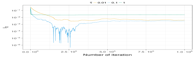
(a)

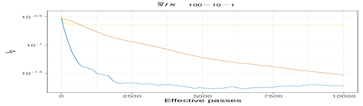
(b)

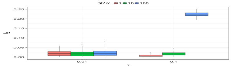
(c)

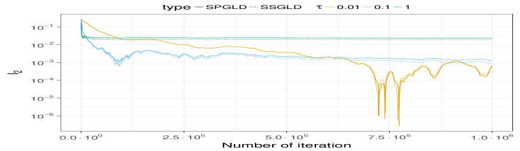
(d)

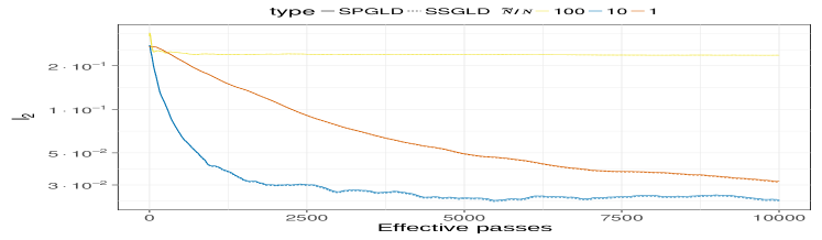
(e)

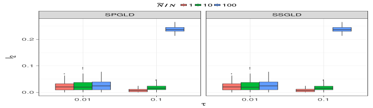
(f)

Figure 1: Mean absolute error of estimator of $I_{2}$ for Australian Credit Approval dataset: (top row) results for $\mathrm{p}_{1,2}(\cdot|(X,Y)_{i\in\{1,\ldots,N\}})$; (a) convergence of SPGLD for $\tilde{N}=1$ , (b) convergence of SPGLD in terms of effective passes for $\tau=0.1$, (c) boxplot of SPGLD for full runs; (bottom row) results for $\mathrm{p}_{1}(\cdot|(X,Y)_{i\in\{1,\ldots,N\}})$; (d) convergence of SPGLD and SSGLD for $\tilde{N}=N$ , (e) convergence of SPGLD and SSGLD in terms of effective passes for $\tau=0.1$, (f) boxplot of SPGLD and SSGLD for full run

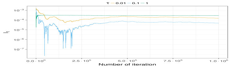
(a)

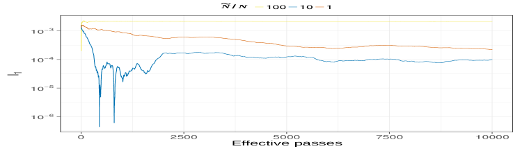
(b)

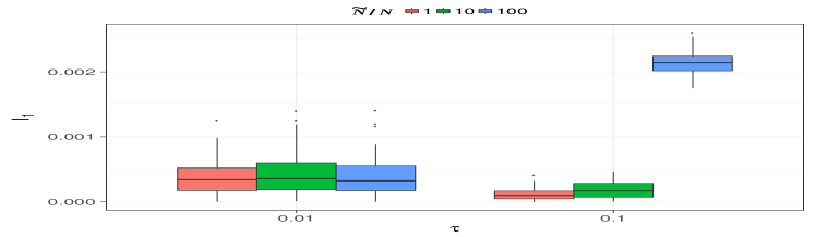
(c)

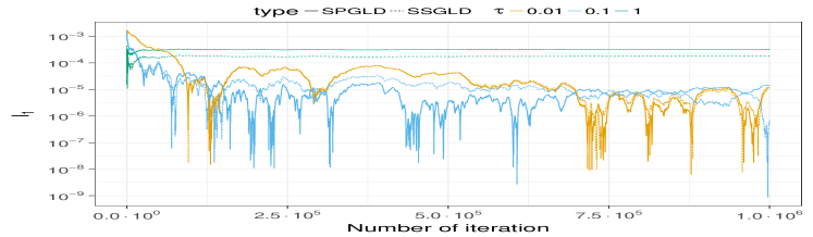
(d)

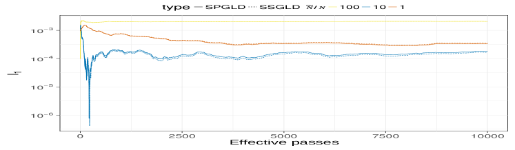
(e)

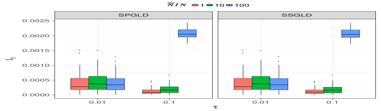
(f)

Figure 2: Mean absolute error of estimator of $I_{1}$ for Australian Credit Approval dataset: (top row) results for $\mathrm{p}_{1,2}(\cdot|(X,Y)_{i\in\{1,\ldots,N\}})$; (a) convergence of SPGLD for $\tilde{N}=1$ , (b) convergence of SPGLD in terms of effective passes for $\tau=0.1$, (c) boxplot of SPGLD for full runs; (bottom row) results for $\mathrm{p}_{1}(\cdot|(X,Y)_{i\in\{1,\ldots,N\}})$; (d) convergence of SPGLD and SSGLD for $\tilde{N}=N$ , (e) convergence of SPGLD and SSGLD in terms of effective passes for $\tau=0.1$, (f) boxplot of SPGLD and SSGLD for full run

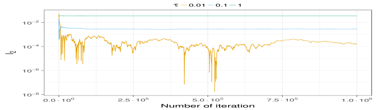
(a)

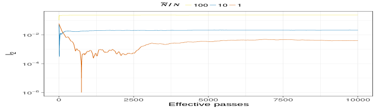
(b)

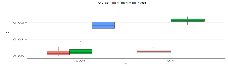
(c)

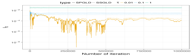
(d)

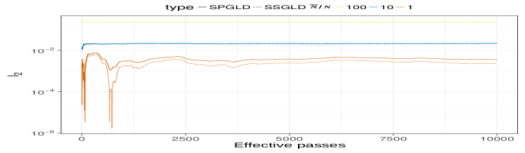
(e)

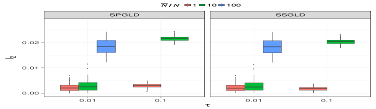
(f)

Figure 3: Mean absolute error of estimator of $I_{2}$ for Heart disease dataset: (top row) results for $\mathrm{p}_{1,2}(\cdot|(X,Y)_{i\in\{1,\ldots,N\}})$; (a) convergence of SPGLD for $\tilde{N}=N$ , (b) convergence of SPGLD in terms of effective passes for $\tau=0.1$, (c) boxplot of SPGLD for full run; (bottom row) results for $\mathrm{p}_{1}(\cdot|(X,Y)_{i\in\{1,\ldots,N\}})$; (d) convergence of SPGLD and SSGLD for $\tilde{N}=N$ , (e) convergence of SPGLD and SSGLD in terms of effective passes for $\tau=0.1$, (f) boxplot of SPGLD and SSGLD for full run

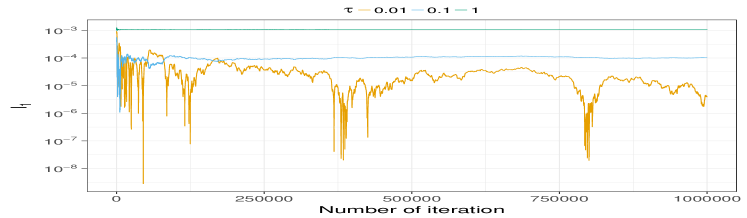
(a)

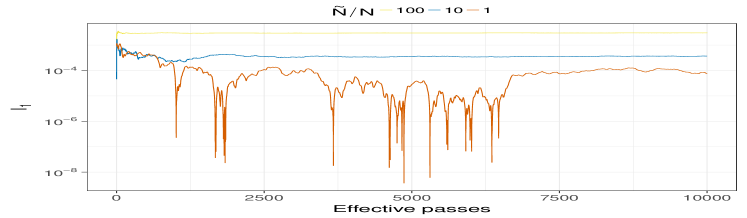
(b)

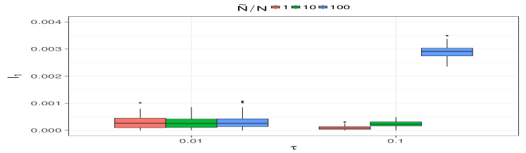
(c)

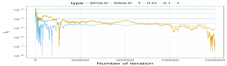
(d)

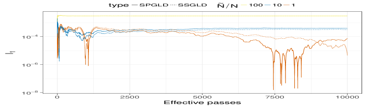
(e)

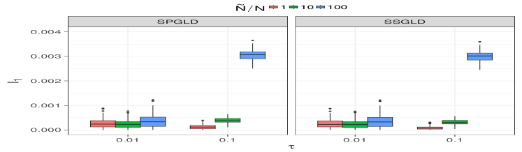
(f)

Figure 4: Mean absolute error of estimator of $I_{1}$ for Heart disease dataset: (top row) results for $\mathrm{p}_{1,2}(\cdot|(X,Y)_{i\in\{1,\ldots,N\}})$; (a) convergence of SPGLD for $\tilde{N}=N$ , (b) convergence of SPGLD in terms of effective passes for $\tau=0.1$, (c) boxplot of SPGLD for full run; (bottom row) results for $\mathrm{p}_{1}(\cdot|(X,Y)_{i\in\{1,\ldots,N\}})$; (d) convergence of SPGLD and SSGLD for $\tilde{N}=N$ , (e) convergence of SPGLD and SSGLD in terms of effective passes for $\tau=0.1$, (f) boxplot of SPGLD and SSGLD for full run

We consider three data sets from UCI repository [14] Heart disease dataset ($N=270$, $d=14$), Australian Credit Approval dataset ($N=690$, $d=34$) and Musk dataset ($N=476$, $d=166$). We approximate $\mathrm{p}_{1}(\cdot|(X,Y)_{i\in\{1,\ldots,N\}})$ using SPGLD and SSGLD, since the associated potential is Lipschitz, whereas regarding $\mathrm{p}_{1,2}(\cdot|(X,Y)_{i\in\{1,\ldots,N\}})$ we only apply SPGLD.

SPGLD is performed using the following stochastic gradient

$$\tilde{\Theta}_{1}(\beta,Z)=(N/\tilde{N})\sum_{n\in Z}\nabla\ell_{n}(\beta)+a_{2}\beta\;,$$

where $a_{2}$ is set to $0$ in the case of $\mathrm{p}_{1}(\cdot|(X,Y)_{i\in\{1,\ldots,N\}})$ and $Z$ is a uniformly distributed random subset of $\{1,\ldots,N\}$ with cardinal $\tilde{N}\in\{1,\ldots,N\}$. In addition, the proximal operator associated with $\beta\mapsto a_{1}\sum_{i=1}^{d}\left|\beta_{i}\right|$ is given for all $\beta\in\mathbb{R}^{d}$ and $\gamma>0$ by (see e.g. [42])

$$(\operatorname{prox}_{a_{1},\ell_{1}}^{\gamma}(\beta))_{i}=\operatorname{sign}(\beta_{i})\max(\left|\beta_{i}\right|-a_{1}\gamma,0)\;,\,\text{ for $i\in\{1,\ldots,d\}$}\;.$$

SSGLD is performed using the following stochastic subgradient

$$\Theta(\beta,Z)=(N/\tilde{N})\sum_{n\in Z}\nabla\ell_{n}(\beta)+a_{1}\sum_{i=1}^{d}\operatorname{sign}(\beta_{i})\mathbf{e}_{i}\;,$$

where $(\mathbf{e}_{i})_{i\in\{1,\ldots,d\}}$ denotes the canonical basis and $Z$ is a uniformly distributed random subset of $\{1,\ldots,N\}$ with cardinal $\tilde{N}\in\{1,\ldots,N\}$.

Based on the results of SPGLD and SSGLD, we estimate the posterior mean $I_{1}$ and $I_{2}$ of the test functions $\beta\mapsto\beta_{1}$ and $\beta\mapsto(1/d)\sum_{i=1}^{d}\beta_{i}^{2}$. For our experiments, we use constant stepsizes $\gamma$ of the form $\tau(L+m)^{-1}$ with $\tau=0.01,0.1,1$ and for stochastic (sub) gradient we use $\tilde{N}=N,\lfloor N/10\rfloor,\lfloor N/100\rfloor$. For all datasets and all settings of $\tau$, $\tilde{N}$ we run $100$ replications of SPGLD (SSGLD), where each run was of length $10^{6}$. For each set of parameters we estimate $I_{1},I_{2}$ and we compute the absolute errors, where the true value were obtained by prox-MALA (see [45]) with $10^{7}$ iterations and stepsize corresponding to optimal acceptance ratio $\approx 0.5$, see [48]. The results for $I_{2}$ are presented on Figure 1, Figure 3 and Figure 5 for Australian Credit Approval dataset, Heart disease dataset and Musk data respectively. The results for $I_{1}$ are presented on Figure 2, Figure 4 and Figure 6 for Australian Credit Approval dataset, Heart disease dataset and Musk data respectively. We note that in the all cases, bias decreases but convergence becomes slower with decreasing $\gamma$. When we look for stochastic (sub)gradient then the bias of estimators and also their variance increase when we decrease $\tilde{N}$. However if we look for effective passes, i.e. number of iteration is scaled with the cost of computing gradients, we observe that convergence is faster with reasonably small $\tilde{N}$. If we compare SSGLD with SPGLD we see that in almost all cases, except Musk dataset, SSGLD leads to slightly smaller bias. For the Musk dataset differences between SSGLD and SPGLD are negligible and we do not present the results for SPGLD. In the presented experiments, all results agrees with our theoretical findings and suggest that SPGLD or SSGLD could be an alternative for other MCMC methods.

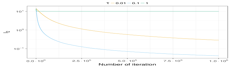
(a)

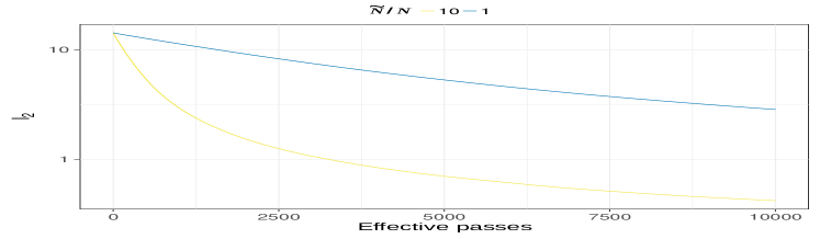
(b)

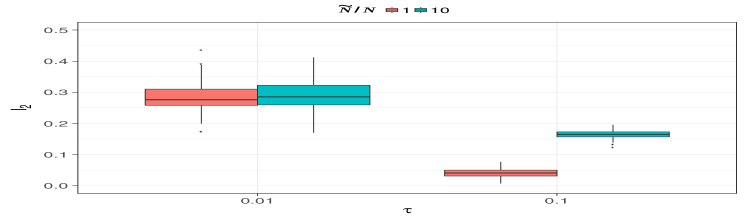
(c)

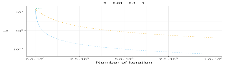
(d)

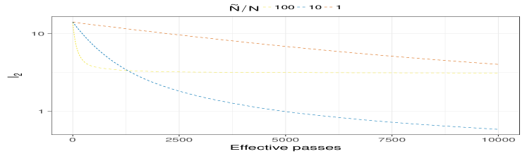
(e)

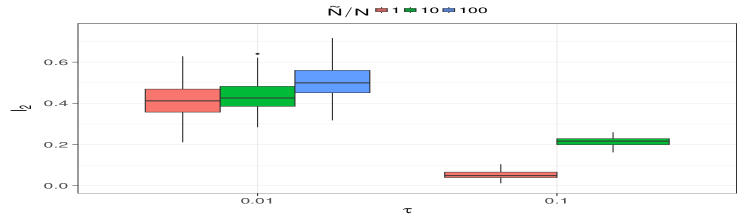
(f)

Figure 5: Mean absolute error of estimator of $I_{2}$ for Musk dataset: (top row) results for $\mathrm{p}_{1-2}$ prior; (a) convergence of SPGLD for $\tilde{N}=1$ , (b) convergence of SPGLD in terms of effective passes for $\tau=0.1$, (c) boxplot of SPGLD for full run; (bottom row) results for $\mathrm{p}_{1}$ prior; (d) convergence of SSGLD for $\tilde{N}=N$ , (e) convergence of SSGLD in terms of effective passes for $\tau=0.1$, (f) boxplot of SSGLD for full run

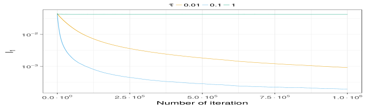
(a)

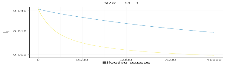
(b)

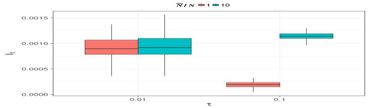
(c)

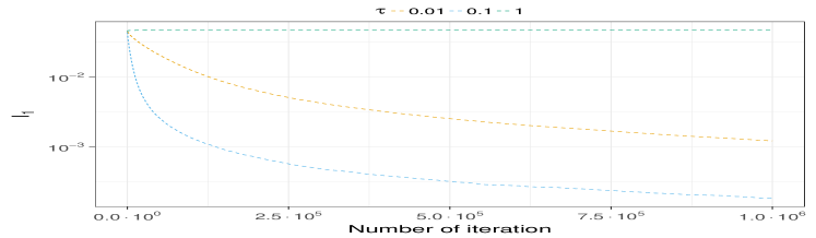
(d)

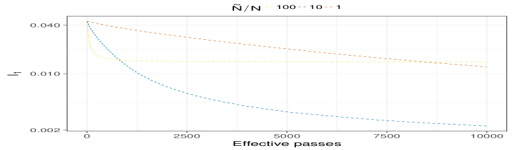
(e)

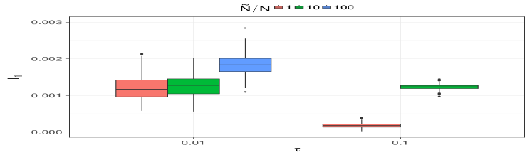
(f)

Figure 6: Mean absolute error of estimator of $I_{1}$ for Musk dataset: (top row) results for $\mathrm{p}_{1-2}$ prior; (a) convergence of SPGLD for $\tilde{N}=1$ , (b) convergence of SPGLD in terms of effective passes for $\tau=0.1$, (c) boxplot of SPGLD for full run; (bottom row) results for $\mathrm{p}_{1}$ prior; (d) convergence of SSGLD for $\tilde{N}=N$ , (e) convergence of SSGLD in terms of effective passes for $\tau=0.1$, (f) boxplot of SSGLD for full run

6 Discussion

In this paper, we presented a novel interpretation of the Unadjusted Langevin Algorithm as a first order optimization algorithm, and a new technique of proving nonasymptotic bounds for ULA, based on the proof techniques known from convex optimization. Our proof technique gives simpler proofs of some of the previously known non-asymptotic results for ULA. It can be also used to prove non-asymptotic bound that were previously unknown. Specifically, to the best of the authors knowledge, we provide the first non-asymptotic results for Stochastic Gradient ULA in the non-strongly convex case, as well as the first non-asymptotic results in the non-smooth non-strongly convex case. Furthermore, our technique extends effortlessly to the stochastic non-smooth case, and to the best of the authors knowledge we provide the first nonasymptotic analysis of that case.

Furthermore our new perspective on the Unadjusted Langevin Algorithm, provides a starting point for further research into connections between Langevin Monte Carlo and Optimization. Specifically, we believe that a very promising direction for further research is translating well known efficient optimization algorithms into efficient sampling algorithms and proving non-asymptotic bounds for those more efficient algorithms.

7 Postponed proofs

7.1 Proof of of Section 2

a) Since $\mathrm{e}^{-U}$ is integrable with respect to the Lebesgue measure, under A 1$(m)$ for $m\geq 0$, by [8, Lemma 2.2.1], there exists $C_{1},C_{2}>0$ such that for all $x\in\mathbb{R}^{d}$, $U(x)\geq C_{1}\left\|x\right\|-C_{2}$. This inequality and A 2 implies that $\pi\in\mathcal{P}_{2}(\mathbb{R}^{d})$. In addition, since the function $x\mapsto U(x)\mathrm{e}^{-U(x)/2}$ is bounded on $[-C_{2},+\infty)$, we have for all $x\in\mathbb{R}^{d}$,

$$\left|\left(U(x)\mathrm{e}^{-U(x)/2}\right)\mathrm{e}^{-U(x)/2}\right|\leq C_{3}\mathrm{e}^{-U(x)/2}$$

for some constant $C_{3}$. From this, and $U(x)\geq C_{1}\left\|x\right\|-C_{2}$ we conclude that $\mathscr{E}(\pi)<+\infty$. Using the same reasoning, we have $\mathscr{H}(\pi)<+\infty$ which finishes the proof of the first part.

b) If $\mu$ does not admit a density with respect to Lebesgue measure, then both sides of (10) are $+\infty$. Second if $\mu$ admits a density still denoted by $\mu$ with respect to the Lebesgue measure, we have by (7):

$$\mathscr{F}(\mu)-\mathscr{F}(\pi)=\operatorname{KL}\left(\mu\middle|\pi\right)+\int_{\mathbb{R}^{d}}\left\{\mu(x)-\pi(x)\right\}\left\{U(x)+\log(\pi(x))\right\}\mathrm{d}x=\operatorname{KL}\left(\mu\middle|\pi\right)\;.$$

7.2 Proof of Section 3

Using Theorem 1 we first get

$$\operatorname{KL}\left(\nu_{n}\middle|\pi\right)\leq\left.W_{2}^{2}\left(\mu_{0},\pi\right)\middle/(2\Gamma_{0,n})\right.+(Ld/\Gamma_{0,n})\sum_{k=1}^{n}\gamma_{k}^{2}\;.$$ (38)

Note that using a simple integral test, we have $\Gamma_{0,n}\geq C_{1}n^{1-\alpha}$ for some constant $C_{1}\geq 0$. On the other hand, for some constant $C_{2}\geq 0$ we have $\sum_{k=1}^{n}\gamma_{k}^{2}\leq C_{2}(1+n^{1-2\alpha})$ if $\alpha\not=1/2$, and $\sum_{k=1}^{n}\gamma_{k}^{2}\leq C_{2}(1+\log(n))$ if $\alpha=1/2$. Combining all these inequalities in (38) concludes the proof.

7.3 Proofs of Section 4.1

Note that for all $\gamma,\tilde{\gamma}>0$, ${\bar{R}}_{\gamma,\tilde{\gamma}}$ can be decomposed as ${\bar{S}}_{\gamma}T_{\tilde{\gamma}}$ where $T_{\tilde{\gamma}}$ is defined in (14) and ${\bar{S}}_{\gamma}$ is given by (30). Then similarly to the proof of Theorem 1, we first give a preliminary bound on $\mathscr{F}(\mu{\bar{R}}_{\gamma,\tilde{\gamma}})-\mathscr{F}(\pi)$ for $\mu\in\mathcal{P}_{2}(\mathbb{R}^{d})$ and $\gamma,\tilde{\gamma}>0$ as in Section 3.

Lemma .

Assume A 1($0$) and A 3. For all $\gamma>0$ and $\mu\in\mathcal{P}_{2}(\mathbb{R}^{d})$,

$$2\gamma\left\{\mathscr{E}(\mu)-\mathscr{E}(\pi)\right\}\leq W_{2}^{2}(\mu,\pi)-W_{2}^{2}(\mu\bar{S}_{\gamma},\pi)+\gamma^{2}\left\{M^{2}+\upsilon_{\Theta}(\mu)\right\}\;,$$

where $\mathscr{E}$ and $T_{\gamma}$ are defined in (9) and (14) respectively, $\upsilon_{\Theta}(\mu)$ in (29) and $\bar{S}_{\gamma}$ in (30).

Proof.

Let $Z$ be a random variable with distribution $\eta$, $\gamma>0$ and $\mu\in\mathcal{P}_{2}(\mathbb{R}^{d})$. For all $x,y\in\mathbb{R}^{d}$, we have using the definition of $\partial U(x)$ (24) and A 3-(ii)

$$\left\|y-x+\gamma\Theta(x,Z)\right\|^{2}=\left\|y-x\right\|^{2}+2\gamma\left\langle\Theta(x,Z),y-x\right\rangle+\gamma^{2}\left\|\Theta(x,Z)\right\|^{2}$$

$$\qquad\qquad\leq\left\|y-x\right\|^{2}-2\gamma\left\{U(x)-U(y)\right\}+2\gamma\left\langle\Theta(x,Z)-\mathbb{E}\left[\Theta(x,Z)\right],y-x\right\rangle+\gamma^{2}\left\|\Theta(x,Z)\right\|^{2}\;.$$

Let $(X,Y)$ be an optimal coupling between $\mu$ and $\pi$ independent of $Z$. Then by A 3-(ii) and rearranging the terms in the previous inequality, we obtain

$$2\gamma\left\{\mathscr{E}(\mu)-\mathscr{E}(\nu)\right\}\leq W_{2}^{2}(\mu,\pi)-\mathbb{E}\left[\left\|Y-X+\gamma\Theta(X,Z)\right\|^{2}\right]+\gamma^{2}\mathbb{E}\left[\left\|\Theta(X,Z)\right\|^{2}\right]\;.$$

The proof is concluded upon noting that $W_{2}^{2}(\mu\bar{S}_{\gamma},\pi)\leq\mathbb{E}[\left\|Y-X+\gamma\Theta(X,Z)\right\|^{2}]$ and $\mathbb{E}[\left\|\Theta(X,Z)\right\|^{2}]\leq M^{2}+\upsilon_{\Theta}(\mu)$. ∎

Proposition .

Assume A 1($0$) and A 3. For all $\gamma,\tilde{\gamma}>0$ and $\mu\in\mathcal{P}_{2}(\mathbb{R}^{d})$,

$$2\tilde{\gamma}\left\{\mathscr{F}(\mu{\bar{R}}_{\gamma,\tilde{\gamma}})-\mathscr{F}(\pi)\right\}\leq\left\{W_{2}^{2}\left(\mu{\bar{S}}_{\gamma},\pi\right)-W_{2}^{2}\left(\mu{\bar{R}}_{\gamma,\tilde{\gamma}}{\bar{S}}_{\tilde{\gamma}},\pi\right)\right\}+\tilde{\gamma}^{2}\left\{M^{2}+\upsilon_{\Theta}(\mu{\bar{R}}_{\gamma,\tilde{\gamma}})\right\}\;.$$

where $\mathscr{F}$ is defined in (9), $\upsilon_{\Theta}(\mu)$ in (29), ${\bar{R}}_{\gamma,\tilde{\gamma}}$ and ${\bar{S}}_{\gamma}$ in (27) in (30) respectively.

Proof.

Note that by Section 7.3, we have

$$2\tilde{\gamma}\left\{\mathscr{E}(\mu{\bar{R}}_{\gamma,\tilde{\gamma}})-\mathscr{E}(\pi)\right\}\leq W_{2}^{2}\left(\mu{\bar{R}}_{\gamma,\tilde{\gamma}},\pi\right)-W_{2}^{2}\left(\mu{\bar{R}}_{\gamma,\tilde{\gamma}}{\bar{S}}_{\tilde{\gamma}},\pi\right)+\tilde{\gamma}^{2}\left\{M^{2}+\upsilon_{\Theta}(\mu{\bar{R}}_{\gamma,\tilde{\gamma}})\right\}\;.$$ (39)

In addition by Section 3, it holds

$$2\tilde{\gamma}\left\{\mathscr{H}(\mu{\bar{R}}_{\gamma,\tilde{\gamma}})-\mathscr{H}(\pi)\right\}\leq W_{2}^{2}\left(\mu{\bar{S}}_{\gamma},\pi\right)-W_{2}^{2}\left(\mu{\bar{R}}_{\gamma,\tilde{\gamma}},\pi\right)\;.$$

The proof then follows from combining this inequality with (39). ∎

7.3.1 Proof of Theorem 4

By Section 7.3, for all $k\in\mathbb{N}^{*}$, we have

$$\mathscr{F}(\mu\bar{Q}_{\gamma}^{k})-\mathscr{F}(\pi)\leq(2\gamma_{k+1})^{-1}\left\{W_{2}^{2}\left(\mu\bar{Q}_{\gamma}^{k-1}\bar{S}_{\gamma_{k}},\pi\right)-W_{2}^{2}\left(\mu\bar{Q}_{\gamma}^{k}\bar{S}_{\gamma_{k+1}},\pi\right)\right\}\\ +(\gamma_{k+1}/2)\left\{M^{2}+\upsilon_{\Theta}(\mu\bar{Q}_{\gamma}^{k})\right\}\;.$$

Similarly to the proof of Theorem 1 using the convexity of Kullback-Leibler divergence and the condition that $(\lambda_{k}/\gamma_{k+1})_{k\in\mathbb{N}^{*}}$ is non-increasing concludes the proof.

7.3.2 Proof of Section 4.1

On the one hand, using Theorem 4, we get:

$$\operatorname{KL}\left(\tilde{\nu}^{N}_{n}\middle|\pi\right)\leq\left.(2\gamma n)^{-1}W_{2}^{2}\left(\mu_{0}\bar{Q}_{\gamma}^{N}{\bar{S}}_{\gamma},\pi\right)+\gamma M^{2}/2+(\gamma/(2n))\sum_{k=N+1}^{N+n}\upsilon_{\Theta}(\mu_{0}\bar{Q}_{\gamma}^{k})\right.\;.$$

On the other hand, using Section 4.1, we obtain:

$$2\gamma(\tilde{L}^{-1}-\gamma)\left(\sum_{k=N+1}^{N+n}\upsilon_{\Theta}(\mu_{0}\bar{Q}_{\gamma}^{k})\right)\leq\int_{\mathbb{R}^{d}}\left\|x-x^{\star}\right\|^{2}\mathrm{d}\mu_{0}\bar{Q}_{\gamma}^{N+1}(x)\\ -\int_{\mathbb{R}^{d}}\left\|x-x^{\star}\right\|^{2}\mathrm{d}\mu_{0}\bar{Q}_{\gamma}^{N+n+1}+2n\gamma^{2}\upsilon_{\Theta}(\updelta_{x^{\star}})+2n\gamma d\;.$$

Combining the two inequalities above finishes the proof of the first part of Section 4.1. For the second part, first observe that since $\gamma_{\varepsilon}\leq(2\tilde{L})^{-1}$ we have $(2(\tilde{L}^{-1}-\gamma))^{-1}\leq\tilde{L}$. Furthermore, from the definition of $\gamma_{\varepsilon}$ we have $\gamma_{\varepsilon}(\frac{M^{2}}{2}+\tilde{L}d)\leq\varepsilon/4$, as well as $\gamma_{\varepsilon}^{2}\tilde{L}\upsilon_{\Theta}(\updelta_{x^{\star}})\leq\varepsilon/4$. On the other hand, from the definition of $n_{\varepsilon}$ we have $W_{2}^{2}(\mu_{0}{\bar{S}}_{\gamma_{\varepsilon}},\pi)/(2\gamma{\varepsilon}n_{\varepsilon})\leq\varepsilon/4$ as well as $\tilde{L}(2n_{\varepsilon})^{-1}\int_{\mathbb{R}^{d}}\left\|x-x^{\star}\right\|^{2}\mathrm{d}\mu_{0}{\bar{R}}_{\gamma_{\varepsilon},\gamma_{\varepsilon}}(x)\leq\varepsilon/4$. Combining those four bounds together finishes the proof.

7.4 Proof of Section 4.2

We proceed for the proof of Theorem 5 similarly to the one of Theorem 1, by decomposing $\mathscr{F}(\mu{\tilde{R}}_{\gamma,\tilde{\gamma}})-\mathscr{F}(\pi)=\mathscr{E}(\mu{\tilde{R}}_{\gamma,\tilde{\gamma}})-\mathscr{E}(\pi)+\mathscr{H}(\mu{\tilde{R}}_{\gamma,\tilde{\gamma}})-\mathscr{H}(\pi)$, for $\mu\in\mathcal{P}_{2}(\mathbb{R}^{d})$ and $\gamma,\tilde{\gamma}>0$. The main difference is that we now need to handle carefully the proximal step in the first term of the decomposition. To this end, we decompose the potential energy functional according to the decomposition of $U$, $\mathscr{E}=\mathscr{E}_{1}+\mathscr{E}_{2}$ where for all $\mu\in\mathcal{P}_{2}(\mathbb{R}^{d})$,

$$\mathscr{E}_{1}(\mu)=\int_{\mathbb{R}^{d}}U_{1}\mathrm{d}\mu(x)\;,\,\qquad\qquad\mathscr{E}_{2}(\mu)=\int_{\mathbb{R}^{d}}U_{2}\mathrm{d}\mu(x)\;,$$ (40)

and consider

$$\mathscr{F}(\mu{\tilde{R}}_{\gamma,\tilde{\gamma}})-\mathscr{F}(\pi)=\mathscr{E}_{1}(\mu{\tilde{R}}_{\gamma,\tilde{\gamma}})-\mathscr{E}_{1}(\mu\tilde{S}_{\gamma}^{2}\tilde{S}_{\tilde{\gamma}}^{1})\\ +\mathscr{E}_{1}(\mu\tilde{S}_{\gamma}^{2}\tilde{S}_{\tilde{\gamma}}^{1})-\mathscr{E}_{1}(\pi)+\mathscr{E}_{2}(\mu{\tilde{R}}_{\gamma,\tilde{\gamma}})-\mathscr{E}_{2}(\pi)+\mathscr{H}(\mu{\tilde{R}}_{\gamma,\tilde{\gamma}})-\mathscr{H}(\pi)\;.$$ (41)

The first and last terms in the right hand side will be controlled using Section 3 and Section 3. In the next lemmas, we bound the other terms separately.

Lemma .

Assume A 5$(m)$, for $m\geq 0$. For all $\mu,\nu\in\mathcal{P}_{2}(\mathbb{R}^{d})$ and $\gamma\in(0,L^{-1}]$,

$$2\gamma\{\mathscr{E}_{1}(\mu\tilde{S}_{\gamma}^{1})-\mathscr{E}_{1}(\nu)\}\leq(1-m\gamma)W_{2}^{2}(\mu,\nu)-W_{2}^{2}(\mu\tilde{S}_{\gamma}^{1},\nu)\\ -\gamma^{2}(1-\gamma L)\int_{\mathbb{R}^{d}}\left\|\nabla U_{1}(x)\right\|^{2}\mathrm{d}\mu(x)+\gamma^{2}(1+\gamma L)\upsilon_{1}(\mu)\;,$$

where $\mathscr{E}_{1},\tilde{S}_{\gamma}^{1}$ is defined by (40)-(33) and $\upsilon_{1}(\mu)$ by (35).

Proof.

Let $\mu,\nu\in\mathcal{P}_{2}(\mathbb{R}^{d})$ and $\gamma>0$. Since $U_{1}$ satisfies A 2 by [39, Lemma 1.2.3], for all $x,\tilde{x}\in\mathbb{R}^{d}$, we have $|U_{1}(\tilde{x})-U_{1}(x)-\left\langle\nabla U_{1}(x),\tilde{x}-x\right\rangle|\leq(L/2)\left\|\tilde{x}-x\right\|^{2}$. Using that $U_{1}$ is $m$-strongly convex by A 5$(m)$, for all $x,y\in\mathbb{R}^{d}$, $z\in\mathsf{Z}$, we get

$$U_{1}(x-\gamma\tilde{\Theta}_{1}(x,z))-U_{1}(y)=U_{1}(x-\gamma\tilde{\Theta}_{1}(x,z))-U_{1}(x)+U_{1}(x)-U_{1}(y)$$

$$\qquad\leq-\gamma\left\langle\nabla U_{1}(x),\tilde{\Theta}_{1}(x,z)\right\rangle+(L\gamma^{2}/2)\left\|\tilde{\Theta}_{1}(x,z)\right\|^{2}+\left\langle\nabla U_{1}(x),x-y\right\rangle-(m/2)\left\|y-x\right\|^{2}\;.$$

Then multiplying both sides by $\gamma$, we obtain

$$2\gamma\left\{U_{1}(x-\gamma\tilde{\Theta}_{1}(x,z))-U_{1}(y)\right\}\leq(1-m\gamma)\left\|x-y\right\|^{2}-\left\|x-\gamma\tilde{\Theta}_{1}(x,z)-y\right\|^{2}\\ -2\gamma^{2}\left\langle\nabla U_{1}(x),\tilde{\Theta}_{1}(x,z)\right\rangle+\gamma^{2}(1+\gamma L)\left\|\tilde{\Theta}_{1}(x,z)\right\|^{2}+2\gamma\left\langle\nabla U_{1}(x)-\tilde{\Theta}_{1}(x,z),x-y\right\rangle\;.$$ (42)

Let now $(X,Y)$ be an optimal coupling between $\mu$ and $\nu$ and $Z$ with distribution $\eta$ independent of $(X,Y)$. Note that A 5 implies that $\mathbb{E}[\tilde{\Theta}_{1}(X,Z)|(X,Y)]=\nabla U_{1}(X)$. Then by definition and (42), we get

$$2\gamma\left\{\mathscr{E}(\mu\tilde{S}^{1}_{\gamma})-\mathscr{E}(\nu)\right\} \leq(1-m\gamma)W_{2}^{2}(\mu,\nu)-\mathbb{E}\left[\left\|X-\gamma\tilde{\Theta}_{1}(X)-Y\right\|^{2}\right]$$

$$\qquad-2\gamma^{2}\mathbb{E}\left[\left\|\nabla U_{1}(X)\right\|^{2}\right]+\gamma^{2}(1+\gamma L)\mathbb{E}\left[\left\|\tilde{\Theta}_{1}(X)\right\|^{2}\right]$$

$$\leq(1-m\gamma)W_{2}^{2}(\mu,\nu)-\mathbb{E}\left[\left\|X-\gamma\tilde{\Theta}_{1}(X)-Y\right\|^{2}\right]$$

$$\qquad-\gamma^{2}(1-\gamma L)\mathbb{E}\left[\left\|\nabla U_{1}(X)\right\|^{2}\right]+\gamma^{2}(1+\gamma L)\upsilon_{1}(\mu)\;.$$

Using that $W^{2}_{2}(\mu\tilde{S}^{1}_{\gamma},\nu)\leq\mathbb{E}[\|X-\gamma\tilde{\Theta}_{1}(X)-Y\|^{2}]$ concludes the proof.

∎

Lemma .

Assume A 5$(m)$ for $m\geq 0$. For all $\mu,\nu\in\mathcal{P}_{2}(\mathbb{R}^{d})$ and $\gamma>0$, we have

$$2\gamma\left\{\mathscr{E}_{2}(\mu)-\mathscr{E}_{2}(\nu)\right\}\leq W_{2}^{2}(\mu,\nu)-W_{2}^{2}(\mu\tilde{S}^{2}_{\gamma},\nu)+2\gamma^{2}M^{2}_{2}\;,$$

where $\mathscr{E}_{2},\tilde{S}^{2}_{\gamma}$ are defined by (40) and (33) respectively.

Proof.

Let $\mu,\nu\in\mathcal{P}_{2}(\mathbb{R}^{d})$ and $\gamma>0$. First we bound for any $x,y\in\mathbb{R}^{d}$, $U_{2}(x)-U_{2}(y)$ using the decomposition $U_{2}(x)-U_{2}(\operatorname{prox}_{U_{2}}^{\gamma}(x))+U_{2}(\operatorname{prox}_{U_{2}}^{\gamma}(x))-U_{2}(y)$. For any $x,y\in\mathbb{R}^{d}$, we have using that $\gamma^{-1}(x-\operatorname{prox}_{U_{2}}^{\gamma}(x))\in\partial U_{2}(\operatorname{prox}_{U_{2}}^{\gamma}(x))$ (see [49, Chapter 1 Section G]), where $\partial U_{2}$ is the sub differential of $U_{2}$ defined by (24),

$$U_{2}(\operatorname{prox}_{U_{2}}^{\gamma}(x))-U_{2}(y)\leq\gamma^{-1}\left\langle x-\operatorname{prox}_{U_{2}}^{\gamma}(x),\operatorname{prox}_{U_{2}}^{\gamma}(x)-y\right\rangle\;.$$

Since $\|x-y\|^{2}=\|x-\operatorname{prox}_{U_{2}}^{\gamma}(x)\|^{2}+\|\operatorname{prox}_{U_{2}}^{\gamma}(x)-y\|^{2}+2\langle x-\operatorname{prox}_{U_{2}}^{\gamma}(x),\operatorname{prox}_{U_{2}}^{\gamma}(x)-y\rangle$, we get for all $x,y\in\mathbb{R}^{d}$,

$$U_{2}(\operatorname{prox}_{U_{2}}^{\gamma}(x))-U_{2}(y)\leq(2\gamma)^{-1}(\|x-y\|^{2}-\|\operatorname{prox}_{U_{2}}^{\gamma}(x)-y\|^{2})\;.$$ (43)

Second, since $U_{2}$ is $M_{2}$-Lipschitz, we get for any $x\in\mathbb{R}^{d}$, $|U_{2}(x)-U_{2}(\operatorname{prox}_{U_{2}}^{\gamma}(x))|\leq M_{2}\|x-\operatorname{prox}_{U_{2}}^{\gamma}(x)\|$. Then using that $\gamma^{-1}(x-\operatorname{prox}_{U_{2}}^{\gamma}(x))\in\partial U_{2}(\operatorname{prox}_{U_{2}}^{\gamma}(x))$, and for any $v\in\partial U_{2}(\operatorname{prox}_{U_{2}}^{\gamma}(x))$, since $U_{2}$ is $M_{2}$-Lipschiz, $\left\|v\right\|\leq M_{2}$, we obtain $|U_{2}(x)-U_{2}(\operatorname{prox}_{U_{2}}^{\gamma}(x))|\leq\gamma M_{2}^{2}$. Combining this result and (43) yields for any $x,y\in\mathbb{R}^{d}$

$$2\gamma\left\{U_{2}(x)-U_{2}(y)\right\}\leq\|x-y\|^{2}-\|\operatorname{prox}_{U_{2}}^{\gamma}(x)-y\|^{2}+2\gamma^{2}M_{2}^{2}\;.$$

Let $(X,Y)$ be an optimal coupling for $\mu$ and $\nu$. The proof then follows from using the inequality above for $(X,Y)$, taking the expectation and because $W_{2}^{2}(\mu\tilde{S}_{\gamma}^{1},\nu)\leq\|\operatorname{prox}_{U_{2}}^{\gamma}(X)-Y\|^{2}$. ∎

Lemma .

Assume A 5$(m)$, for $m\geq 0$. For all $\mu_{0}\in\mathcal{P}_{2}(\mathbb{R}^{d})$ and $\gamma,\tilde{\gamma}\in\left(0,L^{-1}\right]$,

$$2\tilde{\gamma}\{\mathscr{F}(\mu_{0}{\tilde{R}}_{\gamma,\tilde{\gamma}})-\mathscr{F}(\pi)\}\leq(1-m\tilde{\gamma})W_{2}^{2}(\mu_{0}\tilde{S}^{2}_{\gamma},\pi)-W_{2}^{2}(\mu_{0}{\tilde{R}}_{\gamma,\tilde{\gamma}}\tilde{S}^{2}_{\tilde{\gamma}},\pi)\\ +\tilde{\gamma}^{2}\{2Ld+(1+\tilde{\gamma}L)\upsilon_{1}(\mu_{0}\tilde{S}^{2}_{\gamma})+2M_{2}^{2}\}\;,$$

where $\mathscr{F}$, ${\tilde{R}}_{\gamma,\tilde{\gamma}}$ and $\tilde{S}^{2}_{\gamma}$ are defined by (7)-(32)-(33) respectively.

Proof.

Let $\mu_{0}\in\mathcal{P}_{2}(\mathbb{R}^{d})$ and $\gamma,\tilde{\gamma}\in\left(0,L^{-1}\right]$. By Section 3 and since ${\tilde{R}}_{\gamma,\tilde{\gamma}}=\tilde{S}^{2}_{\gamma}\tilde{S}^{1}_{\tilde{\gamma}}T_{\tilde{\gamma}}$, we have

$$\mathscr{E}_{1}(\mu_{0}{\tilde{R}}_{\gamma,\tilde{\gamma}})-\mathscr{E}_{1}(\mu_{0}\tilde{S}_{\gamma}^{2}\tilde{S}_{\tilde{\gamma}}^{1})\leq 2Ld\tilde{\gamma}\;.$$ (44)

By Section 7.4 since $\tilde{\gamma}\leq 1/L$,

$$2\tilde{\gamma}\{\mathscr{E}_{1}(\mu_{0}\tilde{S}_{\gamma}^{2}\tilde{S}_{\tilde{\gamma}}^{1})-\mathscr{E}_{1}(\pi)\}\leq(1-\tilde{\gamma}m)W_{2}^{2}(\mu_{0}\tilde{S}_{\gamma}^{2},\pi)-W_{2}^{2}(\mu_{0}\tilde{S}_{\gamma}^{2}\tilde{S}_{\tilde{\gamma}}^{1},\pi)\\ +\tilde{\gamma}^{2}(1+\tilde{\gamma}L)\upsilon_{1}(\mu_{0}\tilde{S}_{\gamma}^{2})\;.$$ (45)

By Section 7.4, we have

$$2\tilde{\gamma}\{\mathscr{E}_{2}(\mu_{0}{\tilde{R}}_{\gamma,\tilde{\gamma}})-\mathscr{E}_{2}(\pi)\}\leq W_{2}^{2}(\mu_{0}{\tilde{R}}_{\gamma},\pi)-W_{2}^{2}(\mu_{0}{\tilde{R}}_{\gamma,\tilde{\gamma}}\tilde{S}_{\tilde{\gamma}}^{2},\pi)+2\tilde{\gamma}^{2}M_{2}^{2}\;.$$ (46)

Finally by Section 3, we have

$$2\tilde{\gamma}\{\mathscr{H}(\mu_{0}{\tilde{R}}_{\gamma,\tilde{\gamma}})-\mathscr{H}(\pi)\}\leq W_{2}^{2}(\mu_{0}\tilde{S}^{2}_{\gamma}\tilde{S}^{1}_{\tilde{\gamma}},\pi)-W_{2}^{2}(\mu_{0}{\tilde{R}}_{\gamma,\tilde{\gamma}},\pi)\;.$$ (47)

Combining (44)-(45)-(46)-(47) in (41) concludes the proof. ∎

7.4.1 Proof of Theorem 5

Using the convexity of Kullback-Leibler divergence and Section 7.4, we obtain

$$\operatorname{KL}\left(\tilde{\nu}^{N}_{n}\middle|\pi\right)\leq\Lambda_{N,N+n}^{-1}\sum_{k=N+1}^{N+n}\lambda_{k}\operatorname{KL}\left(\mu_{0}\tilde{Q}_{\gamma}^{k}\middle|\pi\right)$$

$$\leq(2\Lambda_{N,N+n})^{-1}\left[\frac{(1-m\gamma_{N+2})\lambda_{N+1}}{\gamma_{N+2}}W_{2}^{2}\left(\mu_{0}\tilde{Q}_{\gamma}^{N}\tilde{S}^{2}_{\gamma_{N+1}},\pi\right)-\frac{\lambda_{N+n}}{\gamma_{N+n+1}}W_{2}^{2}\left(\mu_{0}\tilde{Q}_{\gamma}^{N+n}\tilde{S}^{2}_{\gamma_{N+n+1}},\pi\right)\right.$$

$$\qquad\qquad\left.+\sum_{k=N+1}^{N+n-1}\left\{\frac{(1-m\gamma_{k+2})\lambda_{k+1}}{\gamma_{k+2}}-\frac{\lambda_{k}}{\gamma_{k+1}}\right\}W_{2}^{2}\left(\mu_{0}Q_{\gamma}^{k-1}\tilde{S}^{2}_{\gamma_{k+1}},\pi\right)\right.$$

$$\qquad\qquad\left.+\sum_{k=N+1}^{N+n}\lambda_{k}\gamma_{k+1}\{2Ld+(1+\gamma_{k+1}L)\upsilon_{1}(\mu_{0}Q_{\gamma}^{k}\tilde{S}^{2}_{\gamma_{k}})+2M_{2}^{2}\}\right]\;.$$

We get the thesis using that $\lambda_{k+1}(1-m\gamma_{k+2})/\gamma_{k+2}\leq\lambda_{k}/\gamma_{k+1}$ for all $k\in\mathbb{N}$.

7.4.2 Proof of Section 4.2

Using Theorem 5 we get:

$$\operatorname{KL}\left(\tilde{\nu}^{N}_{n}\middle|\pi\right)\leq\left.W_{2}^{2}\left(\mu_{0}\tilde{Q}_{\gamma}^{N}{\tilde{S}}_{\gamma}^{2},\pi\right)\middle/(2\gamma n)+\gamma(Ld+M_{2}^{2})+\frac{\gamma}{2n}\sum_{k=N+1}^{N+n}(1+\gamma L)\upsilon_{1}(\mu_{0}Q_{\gamma}^{k}\tilde{S}^{2}_{\gamma})\right.$$

and using Section 4.2 we obtain:

$$2\gamma(\tilde{L}^{-1}-\gamma)\left(\sum_{k=N+1}^{N+n}\upsilon_{1}(\mu_{0}Q_{\gamma}^{k}\tilde{S}^{2}_{\gamma})\right)\leq\int_{\mathbb{R}^{d}}\left\|y-x^{\star}\right\|^{2}\mathrm{d}\mu_{0}Q_{\gamma}^{N+1}\tilde{S}^{2}_{\gamma}(y)\\ -\int_{\mathbb{R}^{d}}\left\|y-x^{\star}\right\|^{2}\mathrm{d}\mu_{0}Q_{\gamma}^{N+n+1}\tilde{S}^{2}_{\gamma}(y)+2n\gamma^{2}\upsilon_{1}(\updelta_{x^{\star}})+2n\gamma d\;,$$

Combining the two inequalities above finishes the proof of the first part of Section 4.2. For the second part, observe that since $\gamma_{\varepsilon}\leq L^{-1}$ and $\gamma_{\varepsilon}\leq(2\tilde{L})^{-1}$ we have $(1+\gamma L)(2(\tilde{L}^{-1}-\gamma))^{-1}\leq 2\tilde{L}$. Therefore from definition of $\gamma_{\varepsilon}$ we have $\gamma_{\varepsilon}(Ld+M_{2}^{2}+2\tilde{L}d)\leq\varepsilon/4$, as well as $\gamma_{\varepsilon}^{2}2\tilde{L}\upsilon_{1}(\updelta_{x^{\star}})\leq\varepsilon/4$. On the other hand, from definition of $n_{\varepsilon}$ we have $W_{2}^{2}(\mu_{0}{\tilde{S}}_{\gamma_{\varepsilon}}^{2},\pi)/(2n_{\varepsilon}\gamma_{\varepsilon})\leq\varepsilon/4$ as well as $2\tilde{L}(2n_{\varepsilon})^{-1}\int_{\mathbb{R}^{d}}\left\|x-x^{\star}\right\|^{2}\mathrm{d}\mu_{0}\tilde{S}^{2}_{\gamma}(y)\leq\varepsilon/4$. Combining this four bounds we get the thesis.

7.4.3 Proof of Theorem 6

Using Section 7.4 and since the Kullback-Leibler divergence is non-negative, we get for all $k\in\{1,\ldots,n\}$,

$$W_{2}^{2}\left(\mu_{0}\tilde{Q}_{\gamma}^{k}\tilde{S}^{2}_{\gamma_{k+1}},\pi\right)\leq(1-m\gamma_{k+1})W_{2}^{2}\left(\mu_{0}Q_{\gamma}^{k-1}\tilde{S}^{2}_{\gamma_{k}},\pi\right)\\ +\gamma_{k+1}^{2}\{2Ld+(1+\gamma_{k+1}L)\upsilon_{1}(\mu_{0}Q_{\gamma}^{k-1}\tilde{S}^{2}_{\gamma_{k}})+2M_{2}^{2}\}\;.$$

The proof then follows from a direct induction.

7.4.4 Proof of Section 4.2

Let $\gamma>0$, $x\in\mathbb{R}^{d}$ and consider $\tilde{X}_{1}=\operatorname{prox}_{U_{2}}^{\gamma}\left\{x-\gamma\tilde{\Theta}_{1}(x,Z_{1})+\sqrt{2\gamma}G_{1}\right\}$, where $Z_{1}$ and $G_{1}$ are two independent random variables, $Z_{1}$ has distribution $\eta_{1}$ and $G_{1}$ is a standard Gaussian random variable, so that $\tilde{X}_{1}$ has distribution $\tilde{S}^{1}_{\gamma}T_{\gamma}\tilde{S}^{2}_{\gamma}(x,\cdot)$. First by [4, Theorem 26.2(vii)], we have that $x^{\star}=\operatorname{prox}_{U_{2}}^{\gamma}(x^{\star}-\gamma\nabla U_{1}(x^{\star}))$ and by [4, Proposition 12.27], the proximal is non-expansive, for all $x,y\in\mathbb{R}^{d}$, $\|\operatorname{prox}^{\gamma}_{U_{2}}(x)-\operatorname{prox}^{\gamma}_{U_{2}}(y)\|\leq\left\|x-y\right\|$. Using these two results and the fact that $\tilde{\Theta}_{1}$ satisfies A 4, we have

$$\mathbb{E}\left[\left\|\tilde{X}_{1}-x^{\star}\right\|^{2}\right]=\mathbb{E}\left[\left\|\operatorname{prox}_{U_{2}}^{\gamma}\left\{x-\gamma\tilde{\Theta}_{1}(x,Z_{1})+\sqrt{2\gamma}G_{1}\right\}-\operatorname{prox}_{U_{2}}^{\gamma}\{x^{\star}-\gamma\nabla U_{1}(x^{\star})\}\right\|^{2}\right]$$

$$\qquad\leq\mathbb{E}\left[\left\|\left(x-\gamma\tilde{\Theta}_{1}(x,Z_{1})+\sqrt{2\gamma}G_{1}\right)-\left(x^{\star}-\gamma\nabla U_{1}(x^{\star})\right)\right\|^{2}\right]$$

$$\qquad\leq\left\|x-x^{\star}\right\|^{2}$$

$$\qquad\qquad+\mathbb{E}\left[2\gamma\left\langle x-x^{\star},\nabla U_{1}(x^{\star})-\tilde{\Theta}_{1}(x,Z_{1})\right\rangle+\gamma^{2}\left\|\nabla U_{1}(x^{\star})-\tilde{\Theta}_{1}(x,Z_{1})\right\|^{2}\right]+2\gamma d$$

$$\qquad\leq(1-\tilde{m}_{1}\gamma)\left\|x-x^{\star}\right\|^{2}-2\gamma(\tilde{L}^{-1}_{1}-\gamma)\mathbb{E}\left[\left\|\tilde{\Theta}_{1}(x,Z_{1})-\tilde{\Theta}_{1}(x^{\star},Z_{1})\right\|^{2}\right]$$

$$\phantom{aaaaaaaaaaaaaaaaaaaaaaaaaaaa}+2\gamma^{2}\mathbb{E}\left[\left\|\tilde{\Theta}_{1}(x^{\star},Z_{1})-\nabla U_{1}(x^{\star})\right\|^{2}\right]+2\gamma d\;.$$

The proof is completed upon noting that $\upsilon_{1}(\updelta_{x})\leq\mathbb{E}[\left\|\Theta(x,Z_{1})-\Theta(x^{\star},Z_{1})\right\|^{2}]$.

7.4.5 Proof of Section 4.2

Using Theorem 6 we get:

$$W_{2}^{2}(\mu_{0}{\tilde{R}}_{\gamma,\gamma}^{n}{\tilde{S}}_{\gamma}^{2},\pi) \leq(1-m\gamma)^{n}W_{2}^{2}(\mu_{0}{\tilde{S}}_{\gamma}^{2},\pi)$$

$$+\gamma^{2}\sum_{k=1}^{n}(1-m\gamma)^{n-k}\left(2Ld+(1+\gamma L)\upsilon_{1}(\mu_{0}{\tilde{R}}_{\gamma,\gamma}^{k}\tilde{S}^{2}_{\gamma})+2M_{2}^{2}\right)$$

$$\leq(1-m\gamma)^{n}W_{2}^{2}(\mu_{0}{\tilde{S}}_{\gamma}^{2},\pi)+2(Ld+M_{2})\gamma/m$$

$$+\gamma^{2}\sum_{k=1}^{n}(1-\tilde{m}\gamma)^{n-k}(1+\gamma L)\upsilon_{1}(\mu_{0}{\tilde{R}}_{\gamma,\gamma}^{k}\tilde{S}^{2}_{\gamma})\;.$$ (48)

In addition, using Section 4.2 and $\gamma\leq(2\tilde{L}_{1})^{-1}$, we have

$$\gamma\tilde{L}_{1}^{-1}\sum_{k=1}^{n}(1-\tilde{m}\gamma)^{n-k}\upsilon_{1}(\mu_{0}{\tilde{R}}_{\gamma,\gamma}^{k}\tilde{S}^{2}_{\gamma})\leq 2\gamma\sum_{k=1}^{n}(1-\tilde{m}\gamma)^{n-k}(\gamma\upsilon_{1}(\updelta_{x^{\star}})+d)\\ +\sum_{k=1}^{n}(1-\tilde{m}\gamma)^{n-k+1}\int_{\mathbb{R}^{d}}\left\|x-x^{\star}\right\|^{2}\mathrm{d}\mu_{0}R_{\gamma,\gamma}^{k}\tilde{S}^{2}_{\gamma}(x)\\ -\sum_{k=1}^{n}(1-\tilde{m}\gamma)^{n-k}\int_{\mathbb{R}^{d}}\left\|x-x^{\star}\right\|^{2}\mathrm{d}\mu_{0}R_{\gamma,\gamma}^{k+1}\tilde{S}^{2}_{\gamma}(x)\;.$$

Combining this result and (48) concludes the proof of (37).

Now, for $\gamma_{\varepsilon},n_{\varepsilon}$ as defined in the thesis of the corollary we have $\gamma_{\varepsilon}\Delta_{1}\leq\varepsilon/4$ and $\Delta_{2}\gamma_{\varepsilon}^{2}\leq\varepsilon/4$. Furthermore, $(1-m\gamma_{\varepsilon})^{n_{\varepsilon}}W_{2}^{2}(\mu_{0}{\tilde{S}}_{\gamma_{\varepsilon}}^{2},\pi)\leq\exp(-n_{\varepsilon}m\gamma_{\varepsilon})W_{2}^{2}(\mu_{0}{\tilde{S}}_{\gamma_{\varepsilon}}^{2},\pi)\leq\varepsilon/4$, and $(1-\gamma_{\varepsilon}\tilde{m})\Delta_{3}\leq\varepsilon/4$ similarly. Together, the above inequalities conclude the proof.

Appendix A Definitions and useful results from theory of gradient flows

Let $I\subset\mathbb{R}$ be an open interval of $\mathbb{R}$ and $(\mu_{t})_{t\in I}$ be a curve on $\mathcal{P}_{2}(\mathbb{R}^{d})$, i.e. a family of probability measures belonging to $\mathcal{P}_{2}(\mathbb{R}^{d})$. $(\mu_{t})_{t\in I}$ is said to be absolutely continuous if there exists $\ell\in\mathrm{L}^{1}(I)$ such that for all $s,t\in I$, $s\leq t$, $W_{2}(\mu_{s},\mu_{t})\leq\int_{s}^{t}\left|\ell\right|(u)\mathrm{d}u$. Denote by $\operatorname{AC}(I)$ the set of absolutely continuous curves on $I$ and

$$\operatorname{AC}_{\text{loc}}(\mathbb{R}^{*}_{+})=\left\{(\mu_{t})_{t\geq 0}\ :\,(\mu_{t})_{t\in I}\in\operatorname{AC}(I)\text{ for any open interval }I\subset\mathbb{R}^{*}_{+}\right\}\;.$$

Note that if $(\mu_{t})_{t\in I}\in\operatorname{AC}(I)$, then for any $\nu\in\mathcal{P}_{2}(\mathbb{R}^{d})$, $t\mapsto W_{2}(\nu,\mu_{t})$ is absolutely continuous on $I$ (as a curve from $I$ to $\mathbb{R}_{+}$). Therefore by [41, Theorem 20.8] and [38, Exercice 4, p.45], $t\mapsto W_{2}(\nu,\mu_{t})$ has derivative for almost all $t\in I$ and there exists $\delta:I\to\mathbb{R}$ satisfying

$$\int_{I}\left|\delta\right|(u)\mathrm{d}u<+\infty\text{ and }W_{2}^{2}(\nu,\mu_{t})-W_{2}^{2}(\nu,\mu_{s})=\int_{s}^{t}\delta(u)\mathrm{d}u\;,\text{ for all }s,t\in I$$ (49)

Let $\mu,\nu\in\mathcal{P}_{2}(\mathbb{R}^{d})$. A constant speed geodesic $(\lambda_{t})_{t\in\left[0,1\right]}$ between $\mu$ and $\nu$ is a curve in $\mathcal{P}_{2}(\mathbb{R}^{d})$ such that $\lambda_{0}=\mu$, $\lambda_{1}=\nu$ and for all for all $s,t\in\left[0,1\right]$, $W_{2}(\lambda_{s},\lambda_{t})=\left|t-s\right|W_{2}(\mu,\nu)$. Note that by the triangle inequality, this definition is equivalent to for all $s,t\in\left[0,1\right]$, $W_{2}(\lambda_{s},\lambda_{t})\leq\left|t-s\right|W_{2}(\mu,\nu)$. Indeed by the triangle inequality and the assumption $W_{2}(\lambda_{s},\lambda_{t})\leq\left|t-s\right|W_{2}(\mu,\nu)$, we have for all $s,t\in\left[0,1\right]$, $s<t$,

$$W_{2}(\mu,\nu)\leq W_{2}(\mu,\lambda_{t})+W_{2}(\lambda_{t},\lambda_{s})+W_{2}(\lambda_{s},\nu)\leq W_{2}(\mu,\nu)\;.$$

Therefore the first inequality is in fact an equality, and therefore using again the assumption for $W_{2}(\mu,\lambda_{t})$ and $W_{2}(\lambda_{s},\nu)$ concludes the proof. By definition of the Wasserstein distance of order $2$, a constant speed geodesic $(\lambda_{t})_{t\in\left[0,1\right]}$ between $\mu$ and $\nu$ is given for all $t\in\left[0,1\right]$ by $\lambda_{t}=(t\operatorname{proj}_{1}+(1-t)\operatorname{proj}_{2})_{\sharp}\zeta$ where $\zeta$ is an optimal transport plan between $\mu$ and $\nu$ and $\operatorname{proj}_{1},\operatorname{proj}_{2}:\mathbb{R}^{2d}\to\mathbb{R}^{d}$ are the projections on the first and last $d$ components respectively.

Let $\mathscr{S}:\mathcal{P}_{2}(\mathbb{R}^{d})\to\left(-\infty,+\infty\right]$. The functional $\mathscr{S}$ is said to be lower semi-continuous if for all $M\in\mathbb{R}$, $\{\mathscr{S}\leq M\}$ is a closed set of $\mathcal{P}_{2}(\mathbb{R}^{d})$ and $m$-geodesically convex for $m\geq 0$ if for any $\mu,\nu\in\mathcal{P}_{2}(\mathbb{R}^{d})$ there exists a constant speed geodesic $(\lambda_{t})_{t\in\left[0,1\right]}$ between $\mu$ and $\nu$ such that for all $t\in\left[0,1\right]$

$$\mathscr{S}(\lambda_{t})\leq t\mathscr{S}(\mu)+(1-t)\mathscr{S}(\nu)-t(1-t)(m/2)W_{2}^{2}(\mu,\nu)\;.$$

If $m=0$, $\mathscr{S}$ will be simply said geodesically convex.

A curve $(\mu_{t})_{t>0}\in\operatorname{AC}_{\text{loc}}(\mathbb{R}^{*}_{+})$ is said to be a gradient flow for the lower semi-continuous and $m$-geodesically convex function $\mathscr{S}:\mathcal{P}_{2}(\mathbb{R}^{d})\to\left(-\infty,+\infty\right]$ if for all $\nu\in\mathcal{P}_{2}(\mathbb{R}^{d})$, $\mathscr{S}(\nu)<+\infty$, and for almost all $t\in\mathbb{R}^{*}_{+}$,

$$(1/2)\delta_{t}+(m/2)W_{2}^{2}(\mu_{t},\nu)\leq\mathscr{S}(\nu)-\mathscr{S}(\mu_{t})\;,$$

where $\delta:\mathbb{R}^{*}_{+}\to\mathbb{R}$ satisfies (49) for all open interval of $\mathbb{R}^{*}_{+}$. We say that $(\mu_{t})_{t\in\mathbb{R}^{*}_{+}}$ starts at $\mu$ if $\lim_{t\to 0}W_{2}(\mu_{t},\mu)=0$ and then set $\mu_{0}=\mu$. By [1, Theorem 11.1.4], there exists at most one gradient flow associated with $\mathscr{S}$.

Consider the functional $\tilde{\mathscr{F}}:\mathcal{P}_{2}(\mathbb{R}^{d})\to\left(-\infty,+\infty\right]$ given by $\tilde{\mathscr{F}}=\mathscr{H}+\tilde{\mathscr{E}}$ where $\mathscr{H}$ is defined by (8) and $\tilde{\mathscr{E}}$ for all $\mu\in\mathcal{P}_{2}(\mathbb{R}^{d})$ by

$$\tilde{\mathscr{E}}(\mu)=\int_{\mathbb{R}^{d}}V(x)\mathrm{d}\mu(x)\;,$$

where $V:\mathbb{R}^{d}\to\left(-\infty,+\infty\right]$ is a convex lower-semicontinuous function (for all $M\geq 0$, $\{V\leq M\}$ is closed subset of $\mathbb{R}^{d}$) with $\{V<+\infty\}\not=\emptyset$ and the interior of this set non empty as well. By [1, Proposition 9.3.2, Theorem 9.4.12], $\tilde{\mathscr{F}}$ is geodesically convex and [1, Theorem 11.2.8,Theorem 11.1.4] shows that there exists a unique gradient flow $(\mu_{t})_{t\geq 0}$ starting at $\mu\in\mathcal{P}_{2}(\mathbb{R}^{d})$ and this curve is the unique solution of the Fokker-Plank equation (in the sense of distributions) :

$$\frac{\partial\mu_{t}}{\partial t}=\operatorname{div}(\nabla\mu_{t}^{x}+\mu_{t}^{x}\nabla V(x))\;,$$

i.e. for all $\phi\in C_{c}^{\infty}(\mathbb{R}^{d})$ and $t>0$,

$$\frac{\partial}{\partial t}\int_{\mathbb{R}^{d}}\phi(y)\mu_{t}(\mathrm{d}y)=\int_{\mathbb{R}^{d}}\mathcal{A}\phi(y)\,\mu_{t}(\mathrm{d}y)\;.$$

In addition for all $t>0$, $\mu_{t}$ is absolutely continuous with respect to the Lebesgue measure. In particular for $V=0$, we get the following result.

Theorem 7.

For all $\mu\in\mathcal{P}_{2}(\mathbb{R}^{d})$, there exists a unique solution of the Fokker-Plank equation (in the sense of distributions) :

$$\frac{\partial\mu_{t}}{\partial t}=\Delta\mu_{t}\;.$$

In addition $(\mu_{t})_{t\geq 0}\in\operatorname{AC}(\mathbb{R}^{*}_{+})$ and satisfies for almost all $t\in\mathbb{R}^{*}_{+}$,

$$\delta_{t}/2\leq\mathscr{H}(\nu)-\mathscr{H}(\mu_{t})\;,$$

where $\delta_{t}$ is given in (49).

Appendix B On the second order moment of logconcave measures

A 7.

There exist $\eta>0$, $M_{\eta}\geq 0$ such that for all $x\in\mathbb{R}^{d}$, $x\not\in\operatorname{B}(0,M_{\eta})$,

$$U(x)-U(x^{\star})\geq\eta\left\|x-x^{\star}\right\|\;.$$

In this section, we give some bounds on to deal with the distance of the initial condition of the algorithms from $\pi$ in $W_{2}$.

Proposition .

Assume A 1($0$) and A 7. Then, we have

$$\int_{\mathbb{R}^{d}}\left\|x-x^{\star}\right\|^{2}\mathrm{d}\pi(x) \leq 2\eta^{-2}d(1+d)+M_{\eta}^{2}\;.$$

Proof.

Note that under A 7, we have

$$\int_{\mathbb{R}^{d}}\left\|x-x^{\star}\right\|^{2}\mathrm{d}\pi(x)\leq\eta^{-2}\int_{\mathbb{R}^{d}}\left|U(x)-U(x^{\star})\right|^{2}\mathrm{d}\pi(x)+M_{\eta}^{2}$$

$$\leq 2\eta^{-2}\int_{\mathbb{R}^{d}}\left|U(x)+\log(\mathrm{Z})+\mathscr{H}(\pi)\right|^{2}\mathrm{d}\pi(x)+2\eta^{-2}\left|-\mathscr{H}(\pi)-\log(\mathrm{Z})-U(x^{\star})\right|^{2}+M_{\eta}^{2}\;.$$ (50)

where $\mathscr{H}$ is defined by (8) and $\mathrm{Z}=\int_{\mathbb{R}^{d}}\mathrm{e}^{-U(y)}\mathrm{d}y$. Then, by [6, Proposition I.2], $\left|-\mathscr{H}(\pi)-\log(\mathrm{Z})-U(x^{\star})\right|\leq d$ and by [20, Theorem 2.3], (see also [40] and [56]), $\int_{\mathbb{R}^{d}}\left|U(x)+\log(\mathrm{Z})+\mathscr{H}(\pi)\right|^{2}\mathrm{d}\pi(x)\leq d$. Combining these two results in (50) concludes the proof.

∎

References

• [1] L. Ambrosio, N. Gigli, and G. Savaré. Gradient flows: in metric spaces and in the space of probability measures. Springer Science & Business Media, 2008.
• [2] L. Ambrosio, G. Savaré, and L. Zambotti. Existence and stability for fokker–planck equations with log-concave reference measure. Probability Theory and Related Fields, 145(3):517–564, 2009.
• [3] C. Andrieu, N. De Freitas, A. Doucet, and M. I Jordan. An introduction to MCMC for machine learning. Machine learning, 50(1-2):5–43, 2003.
• [4] H. H. Bauschke and P. L. Combettes. Convex Analysis and Monotone Operator Theory in Hilbert Spaces. Springer Publishing Company, Incorporated, 1st edition, 2011.
• [5] A. Beck and M. Teboulle. A fast iterative shrinkage-thresholding algorithm for linear inverse problems. SIAM J. Imaging Sci., 2(1):183–202, 2009.
• [6] S. Bobkov and M. Madiman. The entropy per coordinate of a random vector is highly constrained under convexity conditions. IEEE Transactions on Information Theory, 57(8):4940–4954, Aug 2011.
• [7] F. Bolley, I. Gentil, and A. Guillin. Convergence to equilibrium in Wasserstein distance for Fokker-Planck equations. J. Funct. Anal., 263(8):2430–2457, 2012.
• [8] S. Brazitikos, A. Giannopoulos, P. Valettas, and B.-H. Vritsiou. Geometry of isotropic convex bodies, volume 196. American Mathematical Society Providence, 2014.
• [9] S. Brooks, A. Gelman, G. L. Jones, and X.-L. Meng. Handbook of Markov chain Monte Carlo, 2011.
• [10] X. Cheng and P. Bartlett. Convergence of Langevin MCMC in KL-divergence. arXiv preprint arXiv:1705.09048, 2017.
• [11] T. M. Cover and J. A. Thomas. Elements of information theory. Wiley-Interscience [John Wiley & Sons], Hoboken, NJ, second edition, 2006.
• [12] A. S. Dalalyan. Theoretical guarantees for approximate sampling from smooth and log-concave densities. Journal of the Royal Statistical Society: Series B (Statistical Methodology), pages n/a–n/a, 2016.
• [13] A. S Dalalyan and A. G. Karagulyan. User-friendly guarantees for the Langevin Monte Carlo with inaccurate gradient. arXiv preprint arXiv:1710.00095, 2017.
• [14] D. Dua and K.T. Efi. UCI machine learning repository, 2017.
• [15] A. Durmus and É. Moulines. Supplement to “high-dimensional bayesian inference via the unadjusted langevin algorithm”, 2015. https://hal.inria.fr/hal-01176084/.
• [16] A. Durmus and E. Moulines. High-dimensional Bayesian inference via the Unadjusted Langevin Algorithm. 2016.
• [17] A. Durmus, É. Moulines, and M. Pereyra. Sampling from convex non continuously differentiable functions, when Moreau meets Langevin. In preparation.
• [18] A. Durmus and É. Moulines. Nonasymptotic convergence analysis for the unadjusted langevin algorithm. Ann. Appl. Probab., 27(3):1551–1587, 06 2017.
• [19] S.N. Ethier and T.G. Kurtz. Markov processes: characterization and convergence. Wiley series in probability and mathematical statistics. Probability and mathematical statistics. Wiley, 1986.
• [20] M. Fradelizi, M. Madiman, and L. Wang. Optimal concentration of information content for log-concave densities. In High dimensional probability VII, pages 45–60. Springer, 2016.
• [21] A. Gelman, J. B Carlin, H. S. Stern, and D. B. Rubin. Bayesian data analysis, volume 2. Chapman & Hall/CRC Boca Raton, FL, USA, 2014.
• [22] S. Geman and D. Geman. Stochastic relaxation, Gibbs distributions and the Bayesian restoration of images. 6:721–741, 1984.
• [23] A. Genkin, D. D Lewis, and D. Madigan. Large-scale bayesian logistic regression for text categorization. Technometrics, 49(3):291–304, 2007.
• [24] C. R. Givens and R. M. Shortt. A class of Wasserstein metrics for probability distributions. Michigan Math. J., 31(2):231–240, 1984.
• [25] R. B. Gramacy and N. G. Polson. Simulation-based regularized logistic regression. Bayesian Anal., 7(3):567–590, 09 2012.
• [26] W. K. Hastings. Monte Carlo sampling methods using Markov chains and their applications. Biometrika, 57(1):97–109, April 1970.
• [27] C. C. Holmes and L. Held. Bayesian auxiliary variable models for binary and multinomial regression. Bayesian Anal., 1(1):145–168, 03 2006.
• [28] R. Jordan, D. Kinderlehrer, and F. Otto. The variational formulation of the Fokker-Planck equation. SIAM journal on mathematical analysis, 29(1):1–17, 1998.
• [29] I. Karatzas and S.E. Shreve. Brownian Motion and Stochastic Calculus. Graduate Texts in Mathematics. Springer New York, 1991.
• [30] W. Krauth. Statistical mechanics: algorithms and computations, volume 13. OUP Oxford, 2006.
• [31] D. Lamberton and G. Pagès. Recursive computation of the invariant distribution of a diffusion: the case of a weakly mean reverting drift. Stoch. Dyn., 3(4):435–451, 2003.
• [32] V. Lemaire. Estimation de la mesure invariante d’un processus de diffusion. PhD thesis, Université Paris-Est, 2005.
• [33] Q. Li and N. Lin. The Bayesian elastic net. Bayesian Anal., 5(1):151–170, 2010.
• [34] B. Martinet. Régularisation d’inéquations variationnelles par approximations successives. Rev. Française Informat. Recherche Opérationnelle, 4:154–158, 1970.
• [35] J. C. Mattingly, A. M. Stuart, and D. J. Higham. Ergodicity for SDEs and approximations: locally Lipschitz vector fields and degenerate noise. Stochastic Process. Appl., 101(2):185–232, 2002.
• [36] N. Metropolis, A. W. Rosenbluth, M. N. Rosenbluth, A. H. Teller, and E. Teller. Equations of state calculations by fast computing machines. Journal of Chemical Physics, 23(2):1087–1092, 1953.
• [37] S. Meyn and R. Tweedie. Markov Chains and Stochastic Stability. Cambridge University Press, New York, NY, USA, 2nd edition, 2009.
• [38] D. Mitrovic and D. Zubrinic. Fundamentals of applied functional analysis, volume 91. CRC Press, 1997.
• [39] Y. Nesterov. Introductory Lectures on Convex Optimization: A Basic Course. Applied Optimization. Springer, 2004.
• [40] V.H. Nguyen. Inégalités Fonctionnelles Et Convexité. 2013.
• [41] O.A. Nielsen. An Introduction to Integration and Measure Theory. Wiley-Interscience and Canadian Mathematics Series of Monographs and Texts. Wiley, 1997.
• [42] N. Parikh and S. Boyd. Proximal Algorithms. Foundations and Trends(r) in Optimization. Now Publishers, 2013.
• [43] G. Parisi. Correlation functions and computer simulations. Nuclear Physics B, 180:378–384, 1981.
• [44] M. Y. Park and T. Hastie. $L_{1}$-regularization path algorithm for generalized linear models. J. R. Stat. Soc. Ser. B Stat. Methodol., 69(4):659–677, 2007.
• [45] M. Pereyra. Proximal markov chain monte carlo algorithms. Statistics and Computing, pages 1–16, 2015.
• [46] Maxim Raginsky, Alexander Rakhlin, and Matus Telgarsky. Non-convex learning via stochastic gradient langevin dynamics: a nonasymptotic analysis. arXiv preprint arXiv:1702.03849, 2017.
• [47] G. O. Roberts and R. L. Tweedie. Exponential convergence of Langevin distributions and their discrete approximations. Bernoulli, 2(4):341–363, 1996.
• [48] Gareth O. Roberts and Jeffrey S. Rosenthal. Optimal scaling of discrete approximations to langevin diffusions. Journal of the Royal Statistical Society: Series B (Statistical Methodology), 60(1):255–268, feb 1998.
• [49] R. T. Rockafellar and R. J.-B. Wets. Variational analysis, volume 317 of Grundlehren der Mathematischen Wissenschaften [Fundamental Principles of Mathematical Sciences]. Springer-Verlag, Berlin, 1998.
• [50] T. Rockafeller. Monotone operators and the proximal point algorithm. SIAM J. Control Optimization, 14:877–898, 1976.
• [51] A. M. Stuart. Inverse problems: a Bayesian perspective. Acta Numer., 19:451–559, 2010.
• [52] D. Talay and L. Tubaro. Expansion of the global error for numerical schemes solving stochastic differential equations. Stochastic Anal. Appl., 8(4):483–509 (1991), 1990.
• [53] T. van Erven and P. Harremos. Rényi Divergence and Kullback-Leibler Divergence. IEEE Transactions on Information Theory, 60(7):3797–3820, July 2014.
• [54] C. Villani. Optimal transport : old and new. Grundlehren der mathematischen Wissenschaften. Springer, Berlin, 2009.
• [55] S. J Vollmer, K. C Zygalakis, and Y. W. Teh. Exploration of the (non-) asymptotic bias and variance of stochastic gradient langevin dynamics. Journal of Machine Learning Research, 17(159):1–48, 2016.
• [56] Liyao Wang. Heat capacity bound, energy fluctuations and convexity. Yale University, 2014.
• [57] M. Welling and Y. W. Teh. Bayesian learning via stochastic gradient Langevin dynamics. In Proceedings of the International Conference on Machine Learning, pages 681–688, 2011.
• [58] Pan Xu, Jinghui Chen, and Quanquan Gu. Global convergence of langevin dynamics based algorithms for nonconvex optimization. arXiv preprint arXiv:1707.06618, 2017.
• [59] D. Zhu and P. Marcotte. New classes of generalized monotonicity. Journal of Optimization Theory and Applications, 87(2):457–471, nov 1995.