Abstract

We consider two non-canonical scalar fields (tachyon and DBI) with E-model type of the potential. We study cosmological inflation in these models to find possible $\alpha$-attractors. We show that similar to the canonical scalar field case, in both tachyon and DBI models there is a value of the scalar spectral index in small $\alpha$ limit which is just a function of the e-folds number. However, the value of $n_{s}$ in DBI model is somewhat different from the other ones. We also compare the results with Planck2015 TT, TE, EE+lowP data. The reheating phase after inflation is studied in these models which gives some more constraints on the model’s parameters.
PACS: 98.80.Cq , 98.80.Es
Key Words: Cosmological Inflation, Non-Canonical Scalar Field, Reheating, $\alpha$-Attractor, Observational Constraints

1 Introduction

It is now accepted that the physics of the early universe can be explained by a testable paradigm named cosmological inflation. The simplest realization of the inflation is a model with a canonically-normalized single scalar field which its nearly flat potential dominates the energy density of the universe. In this model, the dominant mode of the primordial density perturbations (seeded by the quantum fluctuations of the scalar field during the inflation era) is predicted to be almost adiabatic and scale invariant and has Gaussian distribution [1, 2, 3, 4, 5, 6, 7, 8, 9]. However, there is a possibility that inflation may be driven by a single field with non-canonical kinetic energy. Usually, the non-canonical inflation models are referred to as “k-inflation”. These models predict that the primordial density perturbations are somehow scale dependent (which is mildly supported by the Planck2015 released data [10, 11]) and have non-Gaussian distribution. Among the k-inflation models, we can mention the DBI and Tachyonic models. In the DBI (Dirac-Born-Infeld) model, the D3 brane moves in a (usually $AdS_{5}$) throat region of a warped compactified space and its radial coordinate identifies the inflaton field [12, 13]. In this model the action involves a non-canonical kinetic term. Also there is a function of the scalar field besides the potential in the action. This function is related to the local geometry of the compact manifold through it the D3 brane traverses. Tachyon field also, is associated to the D-branes in string theory [14, 15, 16]. This field can be responsible for early time inflation in the history of the Universe, as well as, the late time accelerating expansion. Authors have studied some aspects of the tachyon and DBI models in Refs. [17, 18, 19, 20, 21, 22, 23, 24, 25, 26, 27]

The “cosmological attractor” in inflation models is the idea which has attracted much attention recently. There are several models incorporating the idea of cosmological attractors which among them we refer to conformal attractors [28, 29] and $\alpha$-attractors models [30, 31, 32, 33]. In [34, 35, 36, 37, 38, 39, 40, 41] one can find more details on the issue of $\alpha$-attractors. The important issue in the conformal attractor model is that in the large e-folds number ($N$), it has the universal prediction as $n_{s}=1-\frac{2}{N}$ and $r=\frac{12}{N^{2}}$. The $\alpha$-attractor models have two types called E-model and T-model according to the adopted potentials. The potential characterizing the E-model is given by

$$V=V_{0}\Big{[}1-\exp\big{(}-\sqrt{\frac{2\kappa^{2}}{3\alpha}}\phi\big{)}\Big{]}^{2n}\,,$$ (1)

and the potential characterizing the T-model is defined as

$$V=V_{0}\tanh^{2n}\Big{(}\frac{\kappa\phi}{\sqrt{6\alpha}}\Big{)}\,,$$ (2)

with $V_{0}$, $n$ and $\alpha$ being some free parameters. It is shown that a canonical single field $\alpha$-attractor model, in the small $\alpha$ limit predicts $n_{s}=1-\frac{2}{N}$ and $r=\frac{12\alpha}{N^{2}}$. As we see, in small $\alpha$ and large $N$ limit, the prediction of the scalar spectral index in the $\alpha$-attractor models is the same as the prediction in the conformal attractor models. In this limit, the tensor-to-scalar ratio in $\alpha$-attractor models is a function of $\alpha$, whereas, it is independent of $\alpha$ in the conformal attractor models.

In the study of cosmological inflation, the reheating process after the end of inflation is an important issue. The universe inflates as long as the potential is sufficiently flat and the slow-roll conditions $\eta,\epsilon\ll 1$ are satisfied. The inflaton rolls into the minimum of its potential, then as soon as the slow-roll conditions break down and inflation ends it starts to oscillate about the minimum. According to the simple canonical reheating scenario, when inflaton oscillates, it loses energy and by passing the processes which include the physics of particle creation and non-equilibrium phenomena, decays into the plasma of the relativistic particles corresponding to the radiation-dominated Universe [42, 43, 44]. Nevertheless, some authors have proposed other complicated scenarios of reheating including the non-perturbative processes. The instant preheating [45], the parametric resonance decay [46, 47, 48] and tachyonic instability [49, 50, 51, 52, 53, 54] are the examples among the non-perturbative reheating scenarios. Some important parameters, characterizing the reheating epoch, are the e-folds number during reheating ($N_{rh}$) and the reheating temperature ($T_{rh}$). Exploring these parameters during inflation models helps us to find some more constraints on the models parameters [55, 56, 57, 58, 59, 60]. Another useful parameter to study the reheating phase is the effective equation of state parameter during reheating ($\omega_{eff}$). The value of the effective equation of state parameter for a massive inflaton can be $-1$ (if the potential dominates the energy density) and $+1$ (if the kinetic term dominates the energy density). Regarding to this fact that the value of $\omega_{eff}$ at the end of the inflation epoch is $-\frac{1}{3}$ and its value at the beginning of the radiation dominated universe is $\frac{1}{3}$, it seems logical to assume the effective equation of state parameter during the reheating epoch in the range $-\frac{1}{3}\leq\omega_{eff}\leq\frac{1}{3}$. The frequency of the oscillations of the massive inflaton is very larger than the expansion rate at the initial epoch of the reheating, leading to the vanishing averaged effective pressure. In this respect, at the beginning of the reheating epoch the effective equation of state parameter can be considered to be zero, effectively corresponding to the equation of state parameter of the dust matter. After that, when the inflaton oscillates and decays into other particles, the value of $\omega_{eff}$ increases with time and reaches $\frac{1}{3}$, when the radiation dominated era begins. In this regard, this parameter also gives some constraints on the model’s parameters. See also Ref. [61] for a review on reheating.

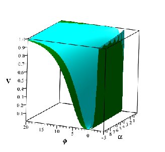
Figure 1: Evolution of the E-model type of potential with $n=1$ (cyan) and $n=2$ (green). For all values of $\alpha$, the potential at large positive values of $\phi$ is nearly flat.

In this paper we consider two inflation models with non-canonical kinetic term: the Tachyon and DBI models. As is clarified in Ref. [13], $f(\phi)$ in DBI model is the warp factor of the AdS throat which for $AdS_{5}$ throat it is equal to $\frac{\lambda}{\phi^{4}}$. Also, if we consider the $AdS_{5}\times X$ geometry, the potential of a DBI field would be quartic. For an approximate AdS throat, there would be a massive scalar field with quadratic potential. On the other hand, in Ref. [62] it has been shown that with $f\sim e^{\lambda\phi}$ and $V\sim e^{-\lambda\phi}$ (with $\lambda$ to be a constant) we can get the Lagrangian of the DBI model. Also, the authors of Ref. [63] have obtained the mentioned functions in the DBI inflation model. In Ref. [16] it has been demonstrated that potential of the tachyon model is proportional to $e^{-\beta\phi}$, where $\beta$ is a constant. Also, some authors have studied tachyon cosmology with power law potential (for instance  [20, 21, 64]) and inverse power law potential [65]. Our motivation in this work was two-folds: firstly we have tried to combine, two successful ingredients of inflationary model-building, that is, non-canonical kinetic terms that facilitate the slow-roll inflation and alpha-attractor potentials that provide robust predictions with the hope to shed more light on these issues. Secondly, this model provides a framework that some of the previous studies are special subclass of the solutions presented here. In this regard, by adopting an E-model potential in both the tachyon and DBI model (and also E-model $f^{-1}(\phi)$ in the DBI model), we are able to cover the mentioned types of the potentials. For instance, in large $\alpha$ limit, we have power law inflation. In small $\alpha$ limit (but not $\alpha\rightarrow 0$) we get the inverse exponential potential. We have similar situation for $f(\phi)$. In large $\alpha$ limit, we have $f^{-1}(\phi)\sim\phi^{2n}$. In small $\alpha$ limit we reach an exponential type of $f(\phi)$. In this regard, to study cosmological dynamics of tachyon and DBI models we adopt E-model type of potential with $n=1$ and $n=2$. As figure 1 shows, this potential at large positive values of the scalar field is nearly flat. By assuming this potential, in section II we obtain the slow roll parameters, the scalar spectral index and the tensor-to-scalar ratio in both non-canonical models. We show that the tachyon inflation model, at large $N$ and small $\alpha$, predicts the same scalar spectral index and tensor-to-scalar ratio as the ones predicted in the canonical single field inflation. However, the DBI model predicts the scalar spectral index somewhat different. We also study the evolution of the tensor-to-scalar ratio versus the scalar spectral index in the background of Planck2015 TT, TE, EE+lowP data. As we shall see, the DBI model with E-model potential and for both $n=1$ and $n=2$, does not lie within the 95$\%$ confidence region of the $n_{s}-r$ plane. In section III, we study the reheating phase in the tachyon and DBI models. We obtain the e-folds number, temperature and effective equation of state during reheating. By comparing with observational data, we constraint the model’s parameters.

2 Inflation

The general action for an inflation model driven by an arbitrary single scalar field is given by

$$S=\int d^{4}x\sqrt{-g}\Bigg{[}\frac{1}{2\kappa^{2}}R+P(X,\phi)\Bigg{]},$$ (3)

where, $R$ is the Ricci scalar and the kinetic energy of the scalar field ($\phi$) is defined as $X=-\frac{1}{2}\partial_{\nu}\phi\,\partial^{\nu}\phi$. To study the cosmological dynamics, the term $P(X,\phi)$ should be specified. This term for the tachyon ($tch$) and DBI models is defined as

$$P_{tch}(X,\phi)=-V(\phi)\sqrt{1-2X}\,,$$ (4)

and

$$P_{DBI}(X,\phi)=-f^{-1}(\phi)\sqrt{1-2f(\phi)X}-V(\phi)\,,$$ (5)

respectively. To proceed, we consider each model separately and study its dynamics.

2.1 Inflation in the tachyon model with E-model potential

In a spatially flat FRW metric, the action (3) with $P(X,\phi)$ defined in (4) leads to the following Friedmann equation

$$H^{2}=\frac{\kappa^{2}}{3}\frac{V}{\sqrt{1-\dot{\phi}^{2}}}\,,$$ (6)

where a dot denotes cosmic time derivative of the parameter. By varying the action (3), by $P(X,\phi)$ defined in (4), with respect to the scalar field, the following equation of motion is obtained

$$\frac{\ddot{\phi}}{1-\dot{\phi}^{2}}+3H\dot{\phi}+\frac{V^{\prime}}{V}=0\,,$$ (7)

where a prime shows derivative with respect to the tachyon field. To have inflation phase, the slow roll parameters, defined as $\epsilon\equiv-\frac{\dot{H}}{H^{2}}$ and $\eta=-\frac{1}{H}\frac{\ddot{H}}{\dot{H}}$, should satisfy the conditions $\epsilon\ll 1$ and $\eta\ll 1$ (meaning that $\dot{\phi}^{2}\ll 1$ and $\ddot{\phi}\ll 3H\dot{\phi}$). In this regard we obtain

$$\epsilon=\frac{1}{2\kappa^{2}}\frac{V^{\prime 2}}{V^{3}}\,,$$ (8)

and

$$\eta=\frac{1}{\kappa^{2}}\left[\frac{V^{\prime\prime}}{V^{2}}-\frac{1}{2}\frac{V^{\prime 2}}{V^{3}}\right]\,,$$ (9)

which in the inflationary era are much smaller than unity and when one of them reaches unity the inflation ends. By using the definition of the e-folds number during inflation as

$$N=\int_{t_{hc}}^{t_{e}}Hdt\,,$$ (10)

with $t_{hc}$ and $t_{e}$ being the time of the horizon crossing and end of inflation respectively, we get the following expression

$$N\simeq\int_{\phi_{hc}}^{\phi_{e}}\frac{-\kappa^{2}V^{2}}{V^{\prime}}d\phi\,.$$ (11)

To obtain the perturbation parameters (the scalar spectral index and tensor-to-scalar ratio), we use the power spectrum defined as

$${\cal{A}}_{s}=\frac{H^{2}}{8\pi^{2}{\cal{W}}_{s}c_{s}^{3}}\,,$$ (12)

where

$${\cal{W}}_{s}=\frac{\dot{\phi}^{2}\,V}{2\big{(}1-\dot{\phi}^{2}\big{)}^{\frac{3}{2}}H^{2}}\,,$$ (13)

and the sound speed is given by

$$c_{s}=\sqrt{1-\dot{\phi}^{2}}\,.$$ (14)

The parameters ${\cal{A}}_{s}$ and ${\cal{W}}_{s}$ are evaluated at the horizon crossing time. The scalar spectral index is obtained by using the power spectrum as follows

$$n_{s}-1=\frac{d\ln{\cal{A}}_{s}}{d\ln k}\Bigg{|}_{c_{s}k=aH}\,,$$ (15)

which gives

$$n_{s}=1-6\epsilon+2\eta\,.$$ (16)

Also, the tensor-to-scalar ratio in this setup is given by

$$r=16c_{s}\epsilon\,.$$ (17)

To see more details about obtaining equations (8)-(17) see Refs. [20, 66, 67, 68].

Now, we study the tachyon model with E-model potential defined in (1). First, we seek for the scalar spectral index and tensor-to-scalar ratio in the large $N$ and small $\alpha$ limit. In this limit, we can rewrite the E-model potential as

$$V=V_{0}\Big{[}1-2n\exp\big{(}-\sqrt{\frac{2\kappa^{2}}{3\alpha}}\phi\big{)}\Big{]}\,.$$ (18)

With this potential, the slow-roll parameter $\epsilon$ takes the following form

$$\epsilon=\frac{4}{3}\,{n}^{2}\frac{\left({{\rm e}^{-\frac{\sqrt{6}}{3}\sqrt{{\frac{{\kappa}^{2}}{\alpha}}}\phi}}\right)^{2}}{\left(1-2\,n{{\rm e}^{-\frac{\sqrt{6}}{3}\sqrt{{\frac{{\kappa}^{2}}{\alpha}}}\phi}}\right)^{3}}\,{\alpha}^{-1}\,.$$ (19)

The value of $\epsilon$ at horizon crossing is obtained by setting $\phi=\phi_{hc}$, where $\phi_{hc}$ is found from equation (11) (in which we assume $\phi_{e}\ll\phi_{hc}$). By substituting the obtained $\phi_{hc}$ and considering that the expression ${{\rm e}^{-\frac{\sqrt{6}}{3}\sqrt{{\frac{{\kappa}^{2}}{\alpha}}}\phi}}$ in the considered limit is very small, we obtain

$$\epsilon=\frac{3}{4}\frac{\alpha}{N^{2}}\,.$$ (20)

The above equation by using the definition (17) leads to

$$r=\frac{12\alpha}{N^{2}}\,,$$ (21)

which is exactly the same as the predicted tensor-to-scalar ratio in the large $N$ and small $\alpha$ limit obtained in the canonical single field inflation. Similarly, for the scalar spectral index, by using $\phi_{hc}$ and equation (16) we find

$$n_{s}=1-\frac{6\,\alpha}{{N}^{2}\left(1-\frac{3}{2}\,{\frac{\alpha}{N}}\right)^{3}}-\frac{2}{{N}\left(1-\frac{3}{2}\,{\frac{\alpha}{N}}\right)^{2}}\,.$$ (22)

The above expression, in the large $N$ and small $\alpha$ limit becomes

$$n_{s}=1-\frac{2}{N}.$$ (23)

In this limit, the scalar spectral index in tachyon model is also the same as the one predicted in the canonical scalar field model.

On the other hand, if we consider $\alpha\rightarrow\infty$, the E-model potential tends to $\phi^{2n}$ leading to

$$\epsilon={\frac{2{n}^{2}}{{\phi}^{2n+2}{\kappa}^{2}}}\,,$$ (24)

and

$$n_{s}=1-4\,{\frac{n\left(2\,n+1\right)}{{\phi}^{2n+2}{\kappa}^{2}}}\,.$$ (25)

To numerical study of the perturbation parameters $r$ and $n_{s}$ and comparing them with observational data, we use equations (17) (where $\epsilon$ is given by equation (8) with potential (1)) and (22). The results are shown in figure 2. As this figure shows, for both $n=1$ and $n=2$ cases, the scalar spectral index and tensor-to-scalar ratio in $\alpha\rightarrow 0$ limit, tend to $n_{s}=0.96$ and $r=0$ (for $N=50$) and $n_{s}=0.966$ and $r=0$ (for $N=60$). In large $\alpha$ limit, the model reaches the tachyon inflation with power law potential. For $n=1$, in the large $\alpha$ limit, we get $\phi^{2}$ tachyon inflation and for $n=2$, we get $\phi^{4}$ tachyon inflation. Note that, the tachyon model with E-model potential (and with both $n=1,2$ and $N=50,60$) for all values of $\alpha$ is consistent with the Planck2015 TT, TE, EE+lowP data.

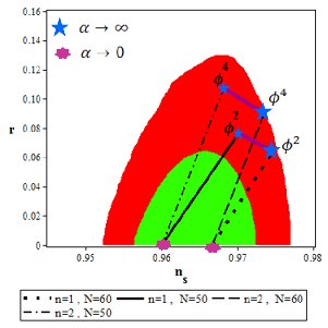
Figure 2: Tensor-to-scalar ratio versus the scalar spectral index for a tachyon model with the E-model potential. The smaller blue stars are corresponding to the tachyon inflation with $\phi^{2n}$ potential and $N=50$ and the larger blue stars are corresponding to the tachyon inflation with $\phi^{2n}$ potential and $N=60$.

2.2 Inflation in the DBI model with E-model potential

Now, we study inflation in the DBI model. The action (3) with $P(X,\phi)$ defined in (5), gives the following Friedmann equation

$$H^{2}=\frac{\kappa^{2}}{3}\Bigg{[}\frac{f^{-1}}{\sqrt{1-f\,\dot{\phi}^{2}}}+V\Bigg{]}\,.$$ (26)

Varying the action (3), by $P(X,\phi)$ defined in (5), with respect to $\phi$ leads to the following equation of motion

$$\frac{\ddot{\phi}}{(1-f\dot{\phi}^{2})^{\frac{3}{2}}}+\frac{3H\dot{\phi}}{(1-f\dot{\phi}^{2})^{\frac{1}{2}}}+V^{\prime}=-\frac{f^{\prime}}{f^{2}}\Bigg{[}\frac{3f\dot{\phi}^{2}-2}{2(1-f\dot{\phi}^{2})^{\frac{1}{2}}}\Bigg{]}.$$ (27)

Inflation occurs when the conditions $\epsilon\ll 1$ and $\eta\ll 1$ (corresponding to $f\dot{\phi}^{2}\ll 1$ and $\ddot{\phi}\ll 3H\dot{\phi}$) are satisfied, where

$$\epsilon={\frac{{f}^{2}{{\it V^{\prime}}}^{2}}{2{\kappa}^{2}\left(Vf+1\right)^{2}}}-{\frac{{\it V^{\prime}}\,{\it f^{\prime}}}{{\kappa}^{2}\left(Vf+1\right)^{2}}}+{\frac{{{\it f^{\prime}}}^{2}}{2{f}^{2}{\kappa}^{2}\left(Vf+1\right)^{2}}}\,,$$ (28)

and

$$\eta=-{\kappa}^{-2}\left(\frac{\left(2\,{\it V^{\prime\prime}}-2\,{\frac{{\it f^{\prime\prime}}}{{f}^{2}}}\right)}{\left(V+{f}^{-1}\right)}-\frac{\left({\it V^{\prime}}-{\frac{{\it f^{\prime}}}{{f}^{2}}}\right)^{2}}{\left(V+{f}^{-1}\right)}\right)\,.$$ (29)

The e-folds number during inflation in DBI model is given by

$$N\simeq\int_{\phi_{hc}}^{\phi_{e}}\frac{\kappa^{2}(V+f^{-1})}{-V^{\prime}+f^{\prime}f^{-2}}d\phi\,.$$ (30)

The power spectrum in this model is given by equation (13) with new definition of ${\cal{W}}$ and $c_{s}$ as

$${\cal{W}}_{s}={\frac{\dot{\phi}^{2}}{2\left(1-f\,\dot{\phi}^{2}\right)^{3/2}H^{2}}}\,,$$ (31)

and

$$c_{s}=\sqrt{1-f\,\dot{\phi}^{2}}\,.$$ (32)

The scalar spectral index and the tensor-to-scalar ratio are given by equations (16) and (17) with the slow-roll parameters defined in (28) and (29).

Similar to the tachyon model, we study the DBI model with E-model potential defined in (1) and

$$f=f_{0}\Big{[}1-\exp\big{(}-\sqrt{\frac{2\kappa^{2}}{3\alpha}}\phi\big{)}\Big{]}^{-2n}\,.$$ (33)

To explore the scalar spectral index and tensor-to-scalar ratio in large $N$ and small $\alpha$ limit, we use the potential (18) and

$$f=f_{0}\Big{[}1+2n\exp\big{(}-\sqrt{\frac{2\kappa^{2}}{3\alpha}}\phi\big{)}\Big{]}\,,$$ (34)

which is written in this limit. With this potential, the slow-roll parameter $\epsilon$ in DBI model is given by the following expression

$$\epsilon=\frac{4}{3}{\alpha}^{-1}\,{n}^{2}{{\rm e}^{-\frac{2}{3}\,{\frac{\sqrt{6}\kappa\,\phi}{\sqrt{\alpha}}}}}\bigg{[}4\,{{\rm e}^{-\frac{4}{3}\,{\frac{\sqrt{6}\kappa\,\phi}{\sqrt{\alpha}}}}}{n}^{4}+8\,{{\rm e}^{-{\frac{\sqrt{6}\kappa\,\phi}{\sqrt{\alpha}}}}}{n}^{3}+8\,{n}^{2}{{\rm e}^{-\frac{2}{3}\,{\frac{\sqrt{6}\kappa\,\phi}{\sqrt{\alpha}}}}}+4\,n{{\rm e}^{-\frac{1}{3}\,{\frac{\sqrt{6}\kappa\,\phi}{\sqrt{\alpha}}}}}+1\bigg{]}\times$$

$$\left[\Big{(}1+2\,n{{\rm e}^{-\frac{1}{3}\,{\frac{\sqrt{6}\kappa\,\phi}{\sqrt{\alpha}}}}}\Big{)}\Big{(}2\,{n}^{2}{{\rm e}^{-\frac{2}{3}\,{\frac{\sqrt{6}\kappa\,\phi}{\sqrt{\alpha}}}}}-1\Big{)}\right]^{-2}\,.\hskip 14.22636pt$$ (35)

By obtaining $\phi_{hc}$ from equation (30), substituting in equation (2.2) and considering that the expression ${\rm e}^{-\frac{2}{3}\,{\frac{\sqrt{6}\kappa\,\phi_{hc}}{\sqrt{\alpha}}}}$ is very small, we get

$$\epsilon=\frac{3}{4}\frac{\alpha}{N^{2}}\,,$$ (36)

which by using equation (17) gives

$$r=\frac{12\alpha}{N^{2}}\,.$$ (37)

We see that, in large $N$ and small $\alpha$ limit, the tensor-to-scalar ratio in DBI model is also the same as the expression predicted for $r$ in the canonical single scalar field model. The scalar spectral index in DBI model takes the following form

$$n_{s}=1-\frac{18\alpha}{N^{2}}\left(\frac{\sqrt{6}}{2N}\,\sqrt{{\frac{{\kappa}^{2}}{\alpha}}}\alpha+1\right)^{-2}+2\,\Bigg{\{}\frac{1}{2}\,\bigg{[}{\frac{6V_{0}{\kappa}^{2}\alpha}{{N}^{2}}}-{\frac{2V_{0}{\kappa}^{2}}{N}}-\frac{3}{2}\,{\frac{V_{0}{\kappa}^{2}\alpha}{n{N}^{2}}}-2\,\bigg{(}\frac{3}{2}\,{\frac{{\kappa}^{2}\alpha}{{N}^{2}V_{0}}}+{\frac{{\kappa}^{2}}{NV_{0}}}$$

$$+\frac{3}{4}\,\frac{{\kappa}^{2}\alpha}{V_{0}{n}{N}^{2}}\Big{(}1-\frac{3}{4}\,{\frac{\alpha}{Nn}}\Big{)}^{-2}\bigg{)}{V}^{2}_{0}\bigg{]}{V}^{-1}_{0}-3/2\,{\frac{{\kappa}^{2}\alpha}{{N}^{2}}}\Bigg{\}}{\kappa}^{-2}\,,\hskip 28.45274pt$$ (38)

where we have assumed $f_{0}^{-1}\equiv V_{0}$ for simplicity. We note that although the functions $V(\phi)$ and $f(\phi)$ are independent, however, both functions are E-model (actually, the inverse of $f(\phi)$ is E-model). In the E-model potential, the coefficient $V_{0}$ is an arbitrary constant. So, when we adopt the E-model for the inverse of $f(\phi)$, the coefficient $f_{0}$ also would be an arbitrary parameter. In this regard, for simplicity, we adopt two constant as $f_{0}^{-1}\equiv V_{0}$. The above scalar spectral index in the large $N$ and small $\alpha$ limit becomes

$$n_{s}=1-\frac{4}{N}.$$ (39)

Here we see that in this limit, the scalar spectral index in DBI model is somewhat different from the tachyon and canonical single field models in the sense that the second term is $\frac{4}{N}$ (whereas in tachyon and canonical single field model is $\frac{2}{N}$). In the $\alpha\rightarrow 0$ limit, $\epsilon$ tends to zero and deviation of $n_{s}$ from the scale invariance comes from the value of $\eta$ in this limit (see equation (16)). In a tachyon model (and also canonical scalar field) $\eta$ is expressed in terms of the potential $V(\phi)$. However, in DBI model, $\eta$ is function of both $V(\phi)$ and $f(\phi)$ (see Eq. (29)) and both these functions contribute in deviation of the scalar spectral index from unity. Considering that these two functions in $\alpha\rightarrow 0$ limit are in the same order, the deviation would be twice. The expression $n_{s}=1-\frac{4}{N}$ has been obtained by the authors of Ref. [64] in a different manner. By a field redefinition and adopting the quartic potential, they obtained this expression for $c_{s}^{2}\ll 1$. However, in the current work, we don’t imply $c_{s}^{2}\ll 1$ limit. We obtain $n_{s}=1-\frac{4}{N}$ by adopting E-model functions and considering $\alpha\rightarrow 0$ limit.

Note that in $\alpha\rightarrow\infty$ limit, the E-model potential tends to $\phi^{2n}$ and we have

$$\epsilon={\frac{8\,{n}^{2}}{{\kappa}^{2}\left(2\,n+\phi\right)^{2}}}\,,$$ (40)

and

$$n_{s}=1-\frac{48\,{n}^{2}}{{\kappa}^{2}\left(2\,{\frac{n}{\phi}}+1\right)^{2}{\phi}^{2}}-{\frac{8n}{{\kappa}^{2}{\phi}^{2}}}\,.$$ (41)

We have performed a numerical study on the perturbation parameters $r$ and $n_{s}$ and the results are shown in figure 3. In this regard, we have used equations (16) and (17) with the slow-roll parameters defined in equations (28) and (29). As figure shows, the DBI model with E-model potential in $\alpha\rightarrow\infty$ limit tends to the DBI model with $\phi^{2n}$ potential. In $\alpha\rightarrow 0$ limit we have $(n_{s}=0.92,r=0)$ for $N=50$ and ($n_{s}=0.933,r=0)$ for $N=60$. The DBI model with E-model potential for both $n=1$ and $n=2$, typically does not lie within the 95$\%$ confidence region of the Planck2015 TT, TE, EE+lowP $r-n_{s}$ result. Nevertheless, the values of the scalar spectral index in the DBI model with $n=1$ and $N=60$, in large $\alpha$ limit, are in $n_{s}=0.9652\pm 0.0047$ range (this range is released by Planck2015 TT, TE, EE+ lowP data).

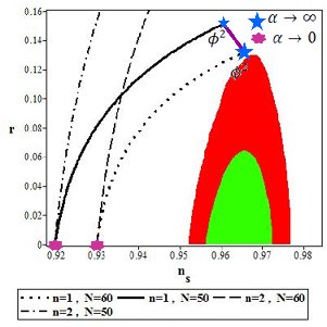
Figure 3: Tensor-to-scalar ratio versus the spectral index for a DBI model with the E-model potential. The smaller blue star is corresponding to DBI inflation with $\phi^{2n}$ potential and $N=50$ while the larger blue star is corresponding to DBI inflation with $\phi^{2n}$ potential and $N=60$.

3 Reheating

When the inflation phase terminates, the process of reheating take places to reheat the universe for subsequent evolution. By studying this process in the aforementioned models, we can find some additional constraints on the model’s parameter space. To this end, we obtain some expressions for $N_{rh}$ and $T_{rh}$ (where subscript rh stands for reheating) in terms of the scalar spectral index based on the strategy presented in Refs. [55, 56, 57, 58, 59]. The following expression

$$N_{hc}=\ln\left(\frac{a_{e}}{a_{hc}}\right)\,,$$ (42)

defines the e-folds number between the time of the horizon crossing of the physical scales and the end of the inflationary expansion. In this definition, $a_{e}$ is the scale factor at the end of the inflation and $a_{hc}$ is the value of the scale factor at the horizon crossing. During the reheating epoch we have the relation $\rho\sim a^{-3(1+\omega_{eff})}$ for the energy density, in which $\omega_{eff}$ is the effective equation of state of the dominant energy density in the universe. In this respect, the e-folds number of the reheating era in terms of the energy density and effective equation of state is written as

$$N_{rh}=\ln\left(\frac{a_{rh}}{a_{e}}\right)=-\frac{1}{3(1+\omega_{eff})}\ln\left(\frac{\rho_{rh}}{\rho_{e}}\right)\,,$$ (43)

By setting the value of $k$ at horizon crossing by $k_{hc}$, we can write

$$0=\ln\left(\frac{k_{hc}}{a_{hc}H_{hc}}\right)=\ln\left(\frac{a_{e}}{a_{hc}}\frac{a_{rh}}{a_{e}}\frac{a_{0}}{a_{rh}}\frac{k_{hc}}{a_{0}H_{hc}}\right)\,,$$ (44)

where $a_{0}$ is the current value of the scale factor. From equations (42), (43) and (44) we obtain

$$N_{hc}+N_{rh}+\ln\left(\frac{k_{hc}}{a_{0}H_{hc}}\right)+\ln\left(\frac{a_{0}}{a_{rh}}\right)=0\,.$$ (45)

In the next step, it is useful to obtain an expression for $\frac{a_{0}}{a}$ in terms of temperature and density. In this regard, we use the following expression

$$\rho_{rh}=\frac{\pi^{2}g_{rh}}{30}T_{rh}^{4}\,,$$ (46)

which gives the relation between energy density and temperature in reheating era [57, 59]. The parameter $g_{rh}$ in equation (46) represents the effective number of the relativistic species at the reheating epoch. On the other hand, from the conservation of the entropy we have [57, 59]

$$\frac{a_{0}}{a_{rh}}=\left(\frac{43}{11g_{rh}}\right)^{-\frac{1}{3}}\frac{T_{rh}}{T_{0}}\,,$$ (47)

where $T_{0}$ denotes the current temperature of the universe. By using equation (46) and (47) we obtain the following expression

$$\frac{a_{0}}{a_{rh}}=\left(\frac{43}{11g_{rh}}\right)^{-\frac{1}{3}}T_{0}^{-1}\left(\frac{\pi^{2}g_{rh}}{30\rho_{rh}}\right)^{-\frac{1}{4}}\,.$$ (48)

To proceed further and to obtain some explicit expressions for $N_{rh}$ and $T_{rh}$, we should specify the model under consideration. In this sense, in what follows we study non-canonical tachyon and DBI models separately.

3.1 Reheating in the tachyon model

In a tachyon model, we can write the energy density in the following form

$$\rho=\frac{V}{\sqrt{1-\frac{2}{3}\epsilon}}\,.$$ (49)

The energy density at the end of inflation era is obtained by setting $\epsilon=1$ as follows

$$\rho_{e}=\sqrt{3}\,V_{e}\,.$$ (50)

Now, by using equations (43) and (50) we obtain

$$\rho_{rh}=\sqrt{3}\,V_{e}\exp\Big{[}-3N_{rh}(1+\omega_{eff})\Big{]}.$$ (51)

From equations (48) and (51) we get

$$\ln\left(\frac{a_{0}}{a_{rh}}\right)=-\frac{1}{3}\ln\left(\frac{43}{11g_{rh}}\right)-\frac{1}{4}\ln\left(\frac{\pi^{2}g_{rh}}{30\rho_{rh}}\right)-\ln T_{0}+\frac{1}{4}\ln\left(\sqrt{3}\,V_{e}\right)-\frac{3}{4}N_{rh}(1+\omega_{eff})\,.\hskip 28.45274pt$$ (52)

By using equation (12), we can find $H_{hc}$. Then, from equations (12), (45) and (52), we obtain the following expression for the e-folds number during reheating

$$N_{rh}=\frac{4}{1-3\omega_{eff}}\Bigg{[}-N_{hc}-\ln\Big{(}\frac{k_{hc}}{a_{0}T_{0}}\Big{)}-\frac{1}{4}\ln\Big{(}\frac{40}{\pi^{2}g_{rh}}\Big{)}-\frac{1}{3}\ln\Big{(}\frac{11g_{rh}}{43}\Big{)}$$

$$+\frac{1}{2}\ln\Big{(}8\pi^{2}{\cal{A}}_{s}{\cal{W}}_{s}c_{s}^{3}\Big{)}-\frac{1}{4}\ln\bigg{(}\sqrt{3}\,V_{e}\bigg{)}\Bigg{]}.$$ (53)

The temperature during reheating is obtained from equations (43), (47) and (50) as follows

$$T_{rh}=\bigg{(}\frac{30}{\pi^{2}g_{rh}}\bigg{)}^{\frac{1}{4}}\,\bigg{[}\sqrt{3}\,V_{e}\bigg{]}^{\frac{1}{4}}\,\exp\bigg{[}-\frac{3}{4}N_{rh}(1+\omega_{eff})\bigg{]}\,.$$ (54)

To perform a numerical study, we should firstly rewrite equations (3.1) and (54) in terms of the scalar spectral index. In this regard, we use equation (1) to rewrite equations (3.1) and (54) in terms of the value of the scalar field at horizon crossing ($\phi_{hc}$). Then, by considering that $\phi_{hc}$ is related to $n_{s}$ (look at equations (1), (8), (9) and (16)), we can write $N_{rh}$ and $T_{rh}$ in terms of $n_{s}$ and then study the reheating phase numerically. The results are shown in figures 4, 5 and 6. In figure 4, we have plotted the ranges of $N_{rh}$ and $\omega_{eff}$ which lead to the observationally viable values of the scalar spectral index. We have considered both $n=1$ and $n=2$ cases for $\alpha=0.1$ and $\alpha\rightarrow\infty$. As figure 4 shows, in all considered cases and with all assumed values of $\omega_{eff}$, the instantaneous reheating (corresponding to $N_{rh}=0$, the point in which all curves converge) is favored by Planck2015 observational data, except for $n=2$ and $\alpha\rightarrow\infty$. The situation is illustrated in figure 5 more explicitly. In this figure we have plotted the e-folds number during reheating versus the scalar spectral index for some sample values of the effective equation of state. Figure 6 shows the temperature during reheating versus the scalar spectral index.

We note that, in an inflation model with a canonical scalar field, the e-folds number and temperature during reheating are defined as equations (3.1) and (54). However, the definitions of some parameters such as $N_{rh}$, ${\cal{A}}_{s}$ and ${\cal{W}}_{s}$ are different in the canonical and non-canonical models. In the tachyon model, these parameters are given by equations (11), (12) and (13). These parameters in a canonical model are defined as $N\simeq-\kappa^{2}\int_{\phi_{hc}}^{\phi_{e}}\frac{V}{V^{\prime}}d\phi$, ${\cal{A}}_{s}=\frac{H^{2}}{8\pi^{2}{\cal{W}}_{s}}$ and ${\cal{W}}_{s}=\frac{\dot{\phi}^{2}}{2H^{2}}$. These definitions cause the different dependence of $N_{rh}$ and $T_{rh}$ to $\phi$ (or $\phi_{hc}$) and therefore to $n_{s}$. For instance, we have the following expression in the canonical model [59]

$$N_{hc}=-\frac{3\alpha}{4n}\Bigg{[}e^{\sqrt{\frac{2\kappa^{2}}{3\alpha}}\phi_{e}}-e^{\sqrt{\frac{2\kappa^{2}}{3\alpha}}\phi_{hc}}-\sqrt{\frac{2\kappa^{2}}{3\alpha}}\left(\phi_{e}-\phi_{hc}\right)\Bigg{]}\,.$$ (55)

The corresponding parameter in the tachyon model is obtained as (see equation (11))

$$N_{hc}=\frac{3\kappa^{2}}{2}\,V_{0}\sqrt{\frac{3\alpha}{2\kappa^{2}}}\left(\phi_{e}-\phi_{hc}\right)-\frac{3}{8}V_{0}\alpha\left({\rm e}^{-2\,{\sqrt{\frac{2\kappa^{2}}{3\alpha}}\,\phi_{e}}}-{\rm e}^{-2{\sqrt{\frac{2\kappa^{2}}{3\alpha}}\,\phi_{hc}}}\right)$$

$$+\frac{9}{4}V_{0}\alpha\left({\rm e}^{-{\sqrt{\frac{2\kappa^{2}}{3\alpha}}\,\phi_{e}}}-{\rm e}^{-\sqrt{\frac{2\kappa^{2}}{3\alpha}}\,\phi_{hc}}\right)-\frac{3}{4}V_{0}\alpha\left({\rm e}^{\sqrt{\frac{2\kappa^{2}}{3\alpha}}\,\phi_{e}}-{\rm e}^{\sqrt{\frac{2\kappa^{2}}{3\alpha}}\,\phi_{hc}}\right)\,.$$ (56)

As we can see, in the canonical model there are terms which are linear and exponential in $\phi$. However, in the tachyon model, there are also some terms which contain the inverse exponential of $\phi$. Such expressions make the numerical results of two model different. Let’s consider the case with $n=1$ and $\alpha=0.1$. With these choices and by adopting $\omega_{eff}=-\frac{1}{3}$, the observational constraint on $N_{rh}$ for the canonical model is as $N_{rh}\leq 4$ (see [59]), while, the corresponding constraint for the tachyon model is as $N_{rh}\leq 26$. By adopting $\omega_{eff}=0$, we have $N_{rh}\leq 8$ for the canonical model [59], and $N_{rh}\leq 52$ for the tachyon model. These mean that, in the non-canonical tachyon model, the reheating phase can last longer than the reheating in the canonical model. We can also compare the temperature during reheating in two models. For $\omega_{ff}=-\frac{1}{3}$ in the canonical model, we have $\log_{10}\left(\frac{T_{rh}}{GeV}\right)>14.3$ [59] and in the tachyon model we have $\log_{10}\left(\frac{T_{rh}}{GeV}\right)>0.9$. If we consider the case with $\omega_{eff}=0$, for the canonical model we have $\log_{10}\left(\frac{T_{rh}}{GeV}\right)>12.8$ [59] and for the tachyon model there is no constraint on the temperature and for any temperature we get the observationally viable $n_{s}$. Here also, we see that in a non canonical tachyon model the larger range of the temperature is corresponding to the observational viable values of $n_{s}$.

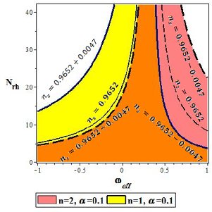
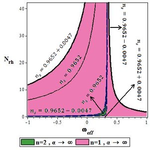
Figure 4: The ranges of the parameters $N_{rh}$ and $\omega_{eff}$ to have observationally viable values of the scalar spectral index for a tachyon model with E-model potential. The left panel corresponds to $\alpha$ =0.1 and the right one is for $\alpha\rightarrow\infty$. Note that in the left panel, the yellow region is bounded by solid lines and the red region is bounded by the dashed lines. The orange overlap region is the range in which both $n=1$ and $n=2$ cases are consistent with observational data. In the right panel, the magenta region is bounded by solid lines and the green region is bounded with dashed lines and is actually the overlap region in this case.

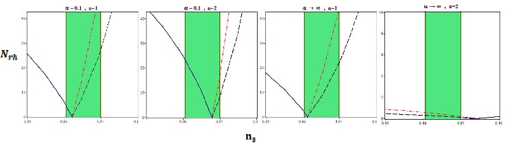
Figure 5: E-folds number during reheating epoch versus the scalar spectral index in a tachyon model with E-model potential. The dashed lines correspond to $\omega_{eff}=-\frac{1}{3}$, the dashed-dotted lines correspond to $\omega_{eff}=0$ and the solid lines correspond to $\omega_{eff}=1$. The green region shows the values of $n_{s}$ released by Planck2015 experiment.

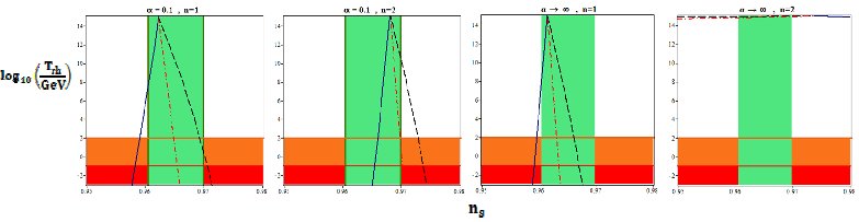
Figure 6: Temperature during reheating epoch versus the scalar spectral index in a tachyon model with E-model potential. The dashed lines correspond to $\omega_{eff}=-\frac{1}{3}$, the dashed-dotted lines correspond to $\omega_{eff}=0$ and the solid lines correspond to $\omega_{eff}=1$. The orange region demonstrates the temperatures below the electroweak scale, $T<100$ GeV and the red region shows the temperatures below the big bang nucleosynthesis scale, $T<10$ MeV.

3.2 Reheating in the DBI model

The energy density in the DBI model can be written as follows

$$\rho=\left(1+\frac{f^{-1}V^{-1}}{\sqrt{1+\frac{2}{3}\epsilon(1+fV)}}\right)V\,.$$ (57)

By setting $\epsilon=1$, we obtain

$$\rho_{e}=\Bigg{(}1+\frac{f_{e}^{-1}V_{e}^{-1}}{\sqrt{1+\frac{2}{3}(1+f_{e}V_{e})}}\Bigg{)}\,.$$ (58)

The energy density during reheating era is obtained from equations (43) and (58) as

$$\rho_{rh}=\Bigg{(}1+\frac{f_{e}^{-1}V_{e}^{-1}}{\sqrt{1+\frac{2}{3}(1+f_{e}V_{e})}}\Bigg{)}\,V_{e}\times\exp\Big{[}-3N_{rh}(1+\omega_{eff})\Big{]}.$$ (59)

Now, equations (48) and (59) give

$$\ln\left(\frac{a_{0}}{a_{rh}}\right)=-\frac{1}{3}\ln\left(\frac{43}{11g_{rh}}\right)-\frac{1}{4}\ln\left(\frac{\pi^{2}g_{rh}}{30\rho_{rh}}\right)-\ln T_{0}+\frac{1}{4}\ln\left[\Bigg{(}1+\frac{f_{e}^{-1}V_{e}^{-1}}{\sqrt{1+\frac{2}{3}(1+f_{e}V_{e})}}\Bigg{)}\,V_{e}\right]$$

$$-\frac{3}{4}N_{rh}(1+\omega_{eff})\,.\hskip 28.45274pt$$ (60)

From equations (12), (45) and (3.2) we obtain

$$N_{rh}=\frac{4}{1-3\omega_{eff}}\Bigg{[}-N_{hc}-\ln\Big{(}\frac{k_{hc}}{a_{0}T_{0}}\Big{)}-\frac{1}{4}\ln\Big{(}\frac{40}{\pi^{2}g_{rh}}\Big{)}-\frac{1}{3}\ln\Big{(}\frac{11g_{rh}}{43}\Big{)}+\frac{1}{2}\ln\Big{(}8\pi^{2}{\cal{A}}_{s}{\cal{W}}_{s}c_{s}^{3}\Big{)}$$

$$-\frac{1}{4}\ln\bigg{(}\bigg{(}1+\frac{f_{e}^{-1}V_{e}^{-1}}{\sqrt{1+\frac{2}{3}(1+f_{e}V_{e})}}\bigg{)}\,V_{e}\bigg{)}\Bigg{]}.\hskip 28.45274pt$$ (61)

Also, from equations (43), (47) and (58) we get

$$T_{rh}=\bigg{(}\frac{30}{\pi^{2}g_{rh}}\bigg{)}^{\frac{1}{4}}\left[\Bigg{(}1+\frac{f_{e}^{-1}V_{e}^{-1}}{\sqrt{1+\frac{2}{3}(1+f_{e}V_{e})}}\Bigg{)}\,V_{e}\right]^{\frac{1}{4}}\times\exp\bigg{[}-\frac{3}{4}N_{rh}(1+\omega_{eff})\bigg{]}\,.\hskip 28.45274pt$$ (62)

By rewriting the equations (3.2) and (62) in terms of the scalar spectral index (similar to what we have done in the tachyon model), we can perform numerical analysis in this model. Note that since the DBI model with E-model potential for $n=2$ is not consistent with the observational data, we don’t study reheating in this case. However, in the $n=1$ case, the scalar spectral index is consistent with observation (although $r$ is not), so we explore reheating in this case. Actually, the observationally viable values of the scalar spectral index can set some constraints on the reheating parameters in DBI model. We remember, for instance, that in a two-field inflation model, one field is responsible for inflation and reheating and the other one is important in perturbations. If we consider DBI as a field responsible for inflation and reheating and not for perturbations in a two-field model, the value of the tensor-to-scalar ratio no matters. In this regard, we think it makes sense to explore the reheating phase for DBI model to see its cosmological consequences. The results are shown in figures 7, 8 and 9. In figure 7 we have plotted the region of the e-folds number during reheating and the effective equation of state for which the scalar spectral index in a DBI model with E-model potential (for $n=1$) is consistent with Planck2015 observational data. As this figure shows, with $\alpha=0.1$ and $n=1$, the instantaneous reheating is disfavored by Planck2015 data for all values of $\omega_{eff}$ (between $-1$ and $+1$). However, with $\alpha\rightarrow\infty$ and $n=1$, for all values of the effective equation of state parameter (varying between $-1$ and $+1$) the instantaneous reheating is favored by observational data. In fact, these results confirm the ones obtained in section 2.2, in the sense that the scalar spectral index (and therefore the e-folds number and temperature during reheating) in large $\alpha$ limit is observationally viable. These situations are clarified also in figure 8. In figure 9 we have plotted the temperature during reheating versus the scalar spectral index.

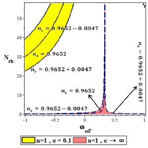
Figure 7: The ranges of the parameters $N_{rh}$ and $\omega_{eff}$ which lead to the observationally viable values of the scalar spectral index for a DBI model with E-model potential.

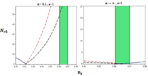
Figure 8: E-folds number during reheating versus the scalar spectral index in a DBI model with E-model potential. The dashed lines correspond to $\omega_{eff}=-\frac{1}{3}$, the dashed-dotted lines correspond to $\omega_{eff}=0$ and the solid lines correspond to $\omega_{eff}=1$. The green region shows the values of $n_{s}$ released by the Planck2015 dataset.

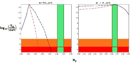
Figure 9: Temperature during reheating versus the scalar spectral index in a DBI model with E-model potential. The dashed lines correspond to $\omega_{eff}=-\frac{1}{3}$, the dashed-dotted lines correspond to $\omega_{eff}=0$ and the solid lines correspond to $\omega_{eff}=1$. The orange region demonstrates the temperatures below the electroweak scale, $T<100$ GeV and the red region shows the temperatures below the big bang nucleosynthesis scale, $T<10$ MeV.

Note that, with $\omega_{eff}=-\frac{1}{3}$, by repeating the analysis performed to obtain equations (3.1), (54), (3.2) and (62) we cannot obtain analytical closed expressions for number of e-folds and temperature. However, a vertical line in the plots can be a curve for $\omega_{eff}=-\frac{1}{3}$ which crosses the instantaneous reheating point [56, 57].

4 Summary and Discussion

In this paper, we have considered two non-canonical scalar field models: tachyon and DBI models. Motivated by the $\alpha$-attractor models, we have adopted the E-model potential to seek for $\alpha$-attractor in these models. We have calculated the slow-roll parameters, scalar spectral index and tensor-to-scalar ratio in both models. The tachyon model with E-model potential in large $N$ and small $\alpha$ limit predicts the value of the scalar spectral index and tensor-to scalar ratio as $n_{s}=1-\frac{2}{N}$ and $r=\frac{12\alpha}{N^{2}}$. These predicted parameters are exactly the same as the ones predicted in the canonical single field model with E-model potential. In $\alpha\rightarrow\infty$ limit, the tachyon model with E-model potential reaches the model with $\phi^{2n}$ potential. We have also analyzed the tachyon model numerically and compared the results with the Planck2015 TT, TE, EE+lowP observational data. We have found that the tachyon model with E-model potential and with both $N=50$ and $N=60$ for all values of $\alpha$ is consistent with the observational data. The $r-n_{s}$ trajectories with a given value of the e-folds number, for both $n=1$ and $n=2$ reaches a fixed point. This means that for $\alpha\rightarrow 0$ the values of the scalar spectral index and tensor-to-scalar ratio are independent of $n$. The value of the scalar spectral index and tensor-to-scalar ratio in small $\alpha$ limit, predicted by DBI model, are as $n_{s}=1-\frac{4}{N}$ and $r=\frac{12\alpha}{N^{2}}$. In DBI model, the calculated $r$ is the same as the one predicted in tachyon and canonical scalar field models. However, $n_{s}$ is somewhat different in the sense that the second term is $\frac{4}{N}$, a factor of 2 different with the corresponding term in tachyon case. Numerical analysis of the DBI model and comparing with the observational data shows that the DBI model with E-model potential does not lie within the 95$\%$ confidence region of the $n_{s}-r$ plane released by Planck2015. But, in large $\alpha$ limit, the value of the scalar spectral index is consistent with observation, though the value of the tensor-to-scalar ratio is not. For $N=50$, the value of $n_{s}$ in the DBI model with $\alpha\rightarrow\infty$ is consistent with Planck2015 TT, TE, EE+lowP observational data. For $N=60$, the value of $n_{s}$ in the DBI model with $\alpha>10^{4}$ is consistent with the observational data.

The reheating era after inflation epoch also has been studied in this paper. For both treated models, we have obtained some expressions for the e-folds number and temperature during the reheating era which give some additional constraints on the model’s parameters space. We have studied the parameters $N_{rh}$, $T_{rh}$ and $\omega_{eff}$ numerically and the results have been shown in figures. By considering the values of the scalar spectral index, allowed by Planck2015 TT, TE, EE+lowP data, we have plotted the regions of $N_{rh}$ and $\omega_{eff}$ which are observationally viable. For tachyon model, we have adopted both $n=1$ and $n=2$ with both $\alpha=0.1$ and $\alpha\rightarrow\infty$. Our numerical analysis shows that, for $n=1$ with both $\alpha=0.1$ and $\alpha\rightarrow\infty$ and for $n=2$ with $\alpha=0.1$, the instantaneous reheating is favored by Planck2015 data. For $n=2$ and $\alpha\rightarrow\infty$, the instantaneous reheating is disfavored by the observational data. We have obtained some constraints by adopting these sample values of the parameters. The constraints on the tachyon model’s parameters, obtained by studying $N_{rh}$ and $n_{s}$ are summarized in table 1.

Table 1: The ranges of the number of e-folds parameter and temperature for tachyon model at reheating which are consistent with observational data.

	$n=1\,\,,\,\,\alpha=0.1$		$n=1\,\,,\,\,\alpha\rightarrow\infty$		$n=2\,\,,\,\,\alpha=0.1$		$n=2\,\,,\,\,\alpha\rightarrow\infty$
$\omega_{eff}=-\frac{1}{3}$	$N_{rh}<26$		$N_{rh}<21$		$N_{rh}<8$		$0.09<N_{rh}<0.026$
$\omega_{eff}=0$	$N_{rh}<52$		$N_{rh}<42$		$N_{rh}<15.5$		$0.2<N_{rh}<0.6$
$\omega_{eff}=1$	$N_{rh}<4.5$		$N_{rh}<1.9$		$N_{rh}<23$		——–
$\omega_{eff}=-\frac{1}{3}$	$\log_{10}\left(\frac{T_{rh}}{GeV}\right)>0.9$		——–		$\log_{10}\left(\frac{T_{rh}}{GeV}\right)>10.6$		$14.97>\log_{10}\left(\frac{T_{rh}}{GeV}\right)>14.93$
$\omega_{eff}=0$	——–		——–		$\log_{10}\left(\frac{T_{rh}}{GeV}\right)>1.8$		——–
$\omega_{eff}=1$	$\log_{10}\left(\frac{T_{rh}}{GeV}\right)>7.4$		$\log_{10}\left(\frac{T_{rh}}{GeV}\right)>8.1$		——–		$\log_{10}\left(\frac{T_{rh}}{GeV}\right)>8.1$

Studying the temperature during reheating era gives some more constraints. The constraints, which are based on the observationally viable values of the scalar spectral index, are presented in table 1.

Regarding that the DBI model with E-model potential and with $n=2$ is not consistent with the observational data, we have performed the numerical analysis on the reheating issue with $n=1$. The numerical study shows that in this model with $n=1$ and $\alpha=0.1$, the instantaneous reheating is disfavored by Planck2015 data (note that, the scalar spectral index also in the case with $n=1$ and $\alpha=0.1$ is disfavored by observational data). However, with $n=1$ and $\alpha\rightarrow\infty$ the instantaneous reheating is favored by the observation. Studying $N_{rh}$ and $T_{rh}$ gives also some more constraints based on the viable values of $n_{s}$, which are summarized in table 2.

Table 2: The ranges of the number of e-folds parameter and temperature for DBI model at reheating which are consistent with observational data.

	$n=1\,\,,\,\,\alpha=0.1$		$n=1\,\,,\,\,\alpha\rightarrow\infty$						$n=1\,\,,\,\,\alpha\rightarrow\infty$
$\omega_{eff}=-\frac{1}{3}$	$49<N_{rh}<80$		$N_{rh}<0.12$						$\log_{10}\left(\frac{T_{rh}}{GeV}\right)>14.9$
$\omega_{eff}=0$	$100<N_{rh}<160$		$N_{rh}<0.25$						$\log_{10}\left(\frac{T_{rh}}{GeV}\right)>14.70$
$\omega_{eff}=1$	——–		$N_{rh}<0.31$						$\log_{10}\left(\frac{T_{rh}}{GeV}\right)>14.77$

For the case with $n=1$ and $\alpha=0.1$, there is no constraint on the reheating temperature.

It seems that if we consider a non-canonical scalar field with the E-model type of potential, the tachyon model is more consistent with observational data than the DBI model. In the tachyon model, the values of the scalar spectral index and tensor-to-scalar ratio for all values of $\alpha$ are consistent with Planck2015 data. Also, there is an attractor point in this model which its scalar spectral index is observationally viable. Exploring the reheating era in this model shows also that this model is observationally viable.

Finally, we note that it would be interesting to think about if one consider some kinetic driven models, like k-inflation [69], and consider the nonminimal coupling term and potential to be E-model. In this case also, we probably get similar attractors. This is because the E-model function and potential in the small $\alpha$ limit tend to a constant and so we probably get some attractors in this limit.

Acknowledgement
We would like to thank the referee for very insightful comments that improved the quality of the paper considerably. This work has been supported financially by Research Institute for Astronomy and Astrophysics of Maragha (RIAAM) under research project number 1/5237-**.

References

- [1] A. Guth, Phys. Rev. D 23, 347 (1981).
- [2] A. D. Linde, Phys. Lett. B 108, 389 (1982)
- [3] A. Albrecht and P. Steinhard, Phys. Rev. D 48, 1220 (1982).
- [4] A. D. Linde, Particle Physics and Inflationary Cosmology (Harwood Academic Publishers, Chur, Switzerland, 1990). [arXiv:hep-th/0503203].
- [5] A. Liddle and D. Lyth, Cosmological Inflation and Large-Scale Structure, (Cambridge University Press, 2000).
- [6] J. E. Lidsey et al, Abney, Rev. Mod. Phys. 69, 373 (1997).
- [7] A. Riotto, [arXiv:hep-ph/0210162].
- [8] D. H. Lyth and A. R. Liddle, The Primordial Density Perturbation (Cambridge University Press, 2009).
- [9] J. M. Maldacena, JHEP 0305, 013 (2003).
- [10] P. A. R. Ade et al., [arXiv:1502.02114] [astro-ph.CO].
- [11] P. A. R. Ade et al., [arXiv:1502.01589] [astro-ph.CO].
- [12] E. Silverstein and D. Tong, Phys. Rev. D 70, 103505 (2004).
- [13] M. Alishahiha, E. Silverstein, and D. Tong, Phys. Rev. D 70, 123505 (2004).
- [14] A. Sen, J. High Energy Phys. 10, 008 (1999).
- [15] A. Sen, J. High Energy Phys. 07, 065 (2002).
- [16] A. Sen, Mod. Phys. Lett. A, 17, 1797 (2002).
- [17] M. Sami, P. Chingangbam, and T. Qureshi, Phys. Rev. D 66, 043530 (2002).
- [18] A. Feinstein, Phys. Rev. D 66, 063511 (2002).
- [19] G.W. Gibbons, Phys. Lett. B 537, 1 (2002).
- [20] K. Nozari and N. Rashidi, Phys. Rev. D 88, 023519 (2013).
- [21] K. Nozari and N. Rashidi, Phys. Rev. D 90, 043522 (2014).
- [22] G. Otalora, Phys. Rev. D 88, 063505 (2013).
- [23] M. x. Huang and G. Shiu, Phys. Rev. D 74, 121301 (2006).
- [24] X. Chen, M. x. Huang, S. Kachru, and G. Shiu, J. Cosmol. Astropart. Phys. 01, 002 (2007).
- [25] K. Nozari and N. Rashidi, Phys. Rev. D 88, 084040 (2013).
- [26] S. Mizuno and K. Koyama, Phys. Rev. D 82, 103518 (2010).
- [27] M. Spalinski, JCAP 0705, 017 (2007).
- [28] R. Kallosh and A. Linde, JCAP 1307, 002 (2013).
- [29] R. Kallosh and A. Linde, JCAP 1312, 006 (2013).
- [30] D. I. Kaiser and E. I. Sfakianakis, Phys. Rev. Lett. 112, 011302 (2014).
- [31] S. Ferrara, R. Kallosh, A. Linde and M. Porrati, Phys. Rev. D 88, 085038 (2013).
- [32] R. Kallosh, A. Linde and D. Roest, JHEP 1311, 198 (2013).
- [33] R. Kallosh, A. Linde and D. Roest, JHEP 1408, 052 (2014).
- [34] S. Cecotti and R. Kallosh, JHEP 05, 114 (2014).
- [35] R. Kallosh, A. Linde and D. Roest, JHEP 09, 062 (2014).
- [36] A. Linde, JCAP 05, 003 (2015).
- [37] J. Joseph, M. Carrasco, R. Kallosh and A. Linde, Phys. Rev. D 92, 063519 (2015).
- [38] J. Joseph, M. Carrasco, R. Kallosh and A. Linde, JHEP 10, 147 (2015).
- [39] R. Kallosh, A. Linde, D. Roest and T. Wrase, JCAP 1611, 046 (2016).
- [40] M. Shahalam, R. Myrzakulov, S. Myrzakul and A. Wang, [arXiv:1611.06315 [astro-ph.CO]].
- [41] S. D. Odintsov and V. K. Oikonomou, Phys. Rev. D 94, 124026 (2016).
- [42] L. F. Abbott, E. Farhi, and M. B. Wise, Phys. Lett. B 117, 29 (1982).
- [43] A. D. Dolgov and A. D. Linde, Phys. Lett. B 116, 329 (1982).
- [44] A. J. Albrecht, P. J. Steinhardt, M. S. Turner and F. Wilczek, Phys. Rev. Lett. 48, 1437 (1982).
- [45] G. N. Felder, L. Kofman, and A. D. Linde, Phys. Rev. D 59, 123523 (1999).
- [46] L. Kofman, A. D. Linde, and A. A. Starobinsky, Phys. Rev. Lett. 73, 3195 (1994) .
- [47] J. H. Traschen and R. H. Brandenberger, Phys. Rev. D 42, 2491 (1990).
- [48] L. Kofman, A. D. Linde, and A. A. Starobinsky, Phys. Rev. D 56 3258 (1997).
- [49] B. R. Greene, T. Prokopec, and T. G. Roos, Phys. Rev. D 56, 6484 (1997).
- [50] N. Shuhmaher and R. Brandenberger, Phys. Rev. D 73, 043519 (2006).
- [51] J. F. Dufaux, G. N. Felder, L. Kofman, M. Peloso, and D. Podolsky, JCAP 0607, 006 (2006).
- [52] A. A. Abolhasani, H. Firouzjahi, and M. Sheikh-Jabbari, Phys. Rev. D 81, 043524 (2010).
- [53] G. N. Felder, J. Garcia-Bellido, P. B. Greene, L. Kofman, A. D. Linde, et al., Phys. Rev. Lett. 87, 011601 (2001) .
- [54] G. N. Felder, L. Kofman, and A. D. Linde, Phys. Rev. D 64, 123517 (2001).
- [55] L. Dai, M. Kamionkowski and J. Wang, Phys. Rev. Lett. 113, 041302 (2014).
- [56] J. B. Munoz and M. Kamionkowski, Phys. Rev. D 91, 043521 (2015).
- [57] J. L. Cook, E. Dimastrogiovanni, D. Easson and L. M. Krauss, JCAP 04, 047 (2015).
- [58] R.-G. Cai, Z.-K. Guo and S.-J. Wang, Phys. Rev. D 92, 063506 (2015).
- [59] Y. Ueno and K. Yamamoto, Phys. Rev. D 93, 083524 (2016).
- [60] K. Nozari and N. Rashidi, Phys. Rev. D 95, 123518 (2017).
- [61] M. A. Amin, M. P. Hertzberg, D. I. Kaiser and J. Karouby , Int. J. Mod. Phys. D 24, 1530003 (2015).
- [62] S. Tsujikawa, J. Ohashi, S. Kuroyanagi and A. De Felice, [arXiv:1305.3044[astro-ph.CO]].
- [63] W. H. Kinney and K. Tzirakis Phys. Rev. D 77, 103517 (2008).
- [64] S. Li and A. R Liddle, DOI: 10.1088/1475-7516/2014/03/044.
- [65] H. Zhang, X.-Z. Li and H. Noh, Phys. Lett. B 691, 1-10 (2010).
- [66] A. De Felice and S. Tsujikawa, Phys. Rev. D 84, 083504 (2011).
- [67] A. De Felice and S. Tsujikawa, JCAP 1104, 029 (2011).
- [68] C. Cheung, P. Creminelli, A. L. Fitzpatrick, J. Kaplan and L. Senatore, JHEP 0803, 014 (2008).
- [69] C. Armendariz-Picon, T. Damour, V. Mukhanov Phys. Lett. B 458, 209 (1999).