A magnetic resonance in high-frequency viscosity of two-dimensional electrons

Abstract

Two-dimensional (2D) electrons in high-quality nanostructures at low temperatures can form a viscous fluid. We develop a theory of high-frequency magnetotransport in such fluid. The time dispersion of viscosity should be taken into account at the frequencies about and above the rate of electron-electron collisions. We show that the shear viscosity coefficients as functions of magnetic field and frequency have the only resonance at the frequency equal to the doubled cyclotron frequency. We demonstrate that such resonance manifests itself in the plasmon damping. Apparently, the predicted resonance is also responsible for the peaks and features in photoresistance and photovoltage, recently observed on the best-quality GaAs quantum wells. The last fact should considered as an important evidence of forming a viscous electron fluid in such structures.

1. Introduction. In solids with enough weak disorder a viscous fluid consisting of phonons or conductive electrons can be formed at low temperatures. For realization of such hydrodynamic regime, the inter-particle collisions conserving momentum must be much more intensive than any other collisions which do not conserve momentum. This idea was proposed many years ago for 3D materials with strong phonon-phonon and electron-phonon interactions Gurzhi ; Gurevich . The hydrodynamic regime of thermal transport in liquid helium and dielectrics was studied in sufficient detail Pitajevkii . However, in those years there existed no enough pure solids where the hydrodynamic regime of charge transport could be realized.

Recently, the crisp fingerprints of forming a 2D viscous electron fluid and realization of hydrodynamic charge transport were discovered in novel ultra-high quality materials: in 3D Weyl semimetals Weyl_sem_1 ; Weyl_sem_2 as well as in 2D nanostructures: graphene grahene ; grahene_2 and GaAs quantum wells je_visc . The most bright of such fingerprints is the giant negative magnetoresistance effect, which was discovered the best-quality GaAs quantum wells exps_neg_1 ; exps_neg_2 ; exps_neg_3 ; exps_neg_4 and on the Weyl semimetal WP₂ Weyl_sem_2 . These experimental discoveries were accompanied by an extensive development of theory Gurzhi_Kalinenko_Kopeliovich ; Spivak ; Andreev ; Mendoza_Herrmann_Succi ; Tomadin_Vignale_Polini ; je_visc ; Levitov_et_al ; Lucas ; eta_xy ; we_1 ; we_2 ; we_3 ; we_4 ; we_5 .

The story of the giant negative magnetoresistance was very bright and non-trivial. Most of the conventional bulk transport theories predict either absent or parabolic positive magnetoresistance. The most well-known bulk mechanism for negative magnetoresistance is the weak localization effect, which leads to a relatively moderate negative magnetoresistance in very weak fields for materials with enough strong disorder. The giant negative magnetoresistance effect, which is the decrease of resistance by 1-2 orders of magnitude in moderate magnetic fields, seemed outstanding, surprising and mysterious during 5 years after its discovering MI_conf .

In Ref. je_visc it was shown that the giant negative magnetoresistance can be explained in details within the hydrodynamic model taking into account the dependence of the electron viscosity coefficients on magnetic field and temperature. By this way, one can consider the best-quality GaAs quantum wells and similar materials as a novel type of solids where the gydridynamic regime of charge transport is realized and the electron viscous fluid flows through a crystal lattice like water through a porous organic material.

In this Letter we provide the second possible evidence that the hydrodynamic regime of charge transport in realized in the ultra-high mobility GaAs quantum wells.

We develop a theory of non-stationary hydrodynamic transport of a 2D viscous electron fluid in magnetic field conf . We derive the Navier-Stocks equation for an ac viscous flow taking into account the time dispersion of viscosity. The obtained frequency-dependent viscosity coefficients have a resonance at the frequency equal to the doubled electron cyclotron frequency, $\omega=2\omega_{c}$, herewith the other harmonics of the cyclotron resonance are absent in the coefficients of the Navier-Stocks equation. So this resonance is a very special type of the high-order cyclotron resonance related to the viscosity effect. It has the following physical nature. A viscous flow is controlled by the diffusive-like transfer of the electron momentum, which is accompanied by the presence of the viscous stress. The last varies in magnetic field as a product of two components of the electron velocity, thus it oscillates with the doubled cyclotron frequency.

We demonstrate that the proposed viscous resonance manifests itself in the damping coefficient of magnetoplasmons and in absorbtion of an ac field by the electron fluid. We also argue that, apparently, the viscous resonance is responsible for the peaks and features at $\omega=2\omega_{c}$ in the photoresistance and the photovoltaic effects, recently observed on the best-quality GaAs quantum wells exp_GaAs_ac_1 ; exp_GaAs_ac_2 ; exp_GaAs_ac_3 . So the viscous resonance together with the giant negative magnetoresistance evidence of forming a viscous electron fluid in moderate magnetic fields in the ultra-pure GaAs quantum wells.

2. Viscous flow in magnetic field. The momentum flux density tensor (per one particle) is defined as: $\Pi_{ij}(\mathbf{r},t)=m\langle v_{i}v_{j}\rangle$, where $m$ is the electron mass, $\mathbf{v}=(v_{x},\,v_{y})$ is the velocity of a single electron and the angular brackets stand for averaging over the electron velocity distribution at a given time $t$ and point $\mathbf{r}=(x,\,y)$. The hydrodynamic velocity in this notations is $V_{i}(\mathbf{r},t)=\langle v_{i}\rangle$. The values $\mathbf{V}$ and $\Pi_{ij}$ are proportional to the first and the second angular harmonics (by the electron velocity vector $\mathbf{v}$) of the electron distribution function $f(\mathbf{v};\mathbf{r},t)$ (see discussion in Refs. LP_Kin ; LL_Hydr ; Steinberg ; Aliev ).

If electrons weakly interact between themselves and can be regarded as an almost ideal Fermi gas, the hydrodynamic approach can be used when the characteristic space scale, $L$, of changing of $\mathbf{V}(\mathbf{r},t)$ is far greater than, at least, one of the following lengths: the electron mean free path relative to electron-electron collisions $l_{ee}=v_{F}\tau_{ee}$; the electron cyclotron radius $R_{c}=v_{F}/\omega_{c}$; the length of the path that free electron passes during the characteristic period of changing of $\mathbf{V}(\mathbf{r},t)$, $l_{\omega}=v_{F}/\omega$. Here $v_{F}$ is the Fermi velocity, $\tau_{ee}$ is the electron-electron scattering time (its exact definition will be clarified below), $\omega_{c}$ is the cyclotron frequency, and $\omega$ is the characteristic frequency of a flow. If one of these conditions is satisfied, then inside the regions of the size $L$ the quasi-equilibrium distribution of electrons is formed and the flow can be described by the values $\mathbf{V}$ and $\Pi_{ij}$.

The equation for the hydrodynamic velocity in zero magnetic flied is:

$$m\frac{\partial V_{i}}{\partial t}=-\frac{\partial\Pi_{ij}}{\partial x_{j}}-\frac{mV_{i}}{\tau}+eE_{i}\>.$$ (1)

Here $e$ is the electron charge, $\tau$ is the momentum relaxation time related to electron scattering on disorder or phonons ph_rates , and summation over repeating indices is assumed. The momentum flux density tensor $\Pi_{ij}$ is equal to $P\delta_{ij}-\sigma_{ij}$, where $P$ is the pressure in the fluid, $\delta_{ij}$ is the Kronecker delta symbol, and $\sigma_{ij}$ is the viscous stress tensor LL_Hydr .

For slow flows which vary at a time scale much greater than the time of relaxation of the inequilibrium part of the momentum flux density tensor, $\Pi_{ij}$ is given by LL_Hydr :

$$\Pi_{ij}^{(0)}=P\delta_{ij}-m\left[\eta\left(V_{ij}-\frac{1}{2}\,\delta_{ij}V_{kk}\right)+\frac{\zeta}{2}\,\delta_{ij}V_{kk}\right]\>,$$ (2)

where $V_{ij}=\partial V_{i}/\partial x_{j}+\partial V_{j}/\partial x_{i}$, $\eta$ are $\zeta$ are the shear and the bulk viscosity coefficients. For the Fermi gas the last is relatively small: $\zeta\sim(T/\varepsilon_{F})^{2}\eta$ zeta_F_zidk , where $T$ is temperature and $\varepsilon_{F}$ is the Fermi energy. In this regard, we will neglect the bulk viscosity in further consideration.

Using Eqs. (1) and (2), one obtains the Navier-Stocks equation in the linear by $\mathbf{V}$ regime:

$$\frac{\partial\mathbf{V}}{\partial t}=\frac{e}{m}\,\mathbf{E}-\frac{\mathbf{V}}{\tau}-\nabla P+\eta\,\Delta\mathbf{V}\>.$$ (3)

In this study we take into account the compressibility of the electron fluid. Thus one needs to supplement Eq. (3) by the gas equation of state $P=P(n)$ (here $n$ is the electron density) and by the continuity equation. The last in the linear regime has the form:

$$\frac{\partial n}{\partial t}+n_{0}\mathrm{div}\mathbf{V}=0\>,$$ (4)

where $n_{0}$ is the unperturbed electron density.

The value given by Eq. (2) is attained during the time $\tau_{ee}$, as described by the Drude-like equation Kaufman :

$$\frac{\partial\Pi_{ij}}{\partial t}=-\frac{1}{\tau_{ee}}\big{(}\Pi_{ij}-\Pi_{ij}^{(0)}\big{)}\>.$$ (5)

Here $\tau_{ee}$ is the time of relaxation of the second angular moment (by the electron velocity) of the electron distribution function. As a rule, it is related to electron-electron scattering. Hydrodynamic effects are significant for an electron fluid in a solid if the scattering on disorder or phonons is much less intensive than electron-electron scattering: $\tau_{ee}\ll\tau$ Gurzhi . Formulas (1), (2), and (5) are the whole system of equations describing nonstationary flows of a 2D viscous electron fluid in zero magnetic field.

For a high-frequency flow with characteristic frequencies $\omega$ compared to $1/\tau_{ee}$ the relation between $\Pi_{ik}(\mathbf{r},t)$ and $V_{ik}(\mathbf{r},t)$ is nonlocal by time. Owing to linearity of the all equations, we can decompose all the values by the time harmonics proportional to $e^{-i\omega t}$. For each pair of harmonic $\mathbf{V}(\mathbf{r},\omega)e^{-i\omega t}$ and $\Pi_{ij}(\mathbf{r},\omega)e^{-i\omega t}$ we obtain from Eq. (1), (2), and (5) the relations between the amplitudes $\mathbf{V}(\mathbf{r},\omega)$ and $\Pi_{ij}(\mathbf{r},\omega)$. This relations have the same form as Eqs. (2) and (3), but contain the amplitude $\mathbf{E}(\mathbf{r},\omega)$ of the electric field harmonic instead of $\mathbf{E}(\mathbf{r},t)$ and the frequency-dependent viscosity coefficient, $\eta(\omega)=\eta/(1-i\omega\tau_{ee}),$ instead of $\eta$.

In the presence of magnetic field additional terms will appear in the equations for $\partial V_{i}/\partial t$ and $\partial\Pi_{ij}/\partial t$, since now the quantities $\langle v_{i}\rangle$ and $\langle v_{i}v_{j}\rangle$ will change in time not only due to collisions and the electric field force, but also due to the magnetic field force. The last force for each electron is $(eB/c)\epsilon_{ikz}v_{k}$, where $\epsilon_{lik}$ is the unit antisymmetric tensor and $z$ is the direction of the magnetic field $\mathbf{B}$, which is perpendicular to the 2D electron layer. For the averaged products of the velocity components in the presence of only the magnetic field $\mathbf{B}$ we have:

$$\begin{array}[]{l}\displaystyle\frac{\partial\langle v_{i}\rangle}{\partial t}=\omega_{c}\epsilon_{ikz}\langle v_{k}\rangle\>,\\ \\ \displaystyle\frac{\partial\langle v_{i}v_{j}\rangle}{\partial t}=\omega_{c}\big{(}\epsilon_{ikz}\langle v_{k}v_{j}\rangle+\epsilon_{jkz}\langle v_{i}v_{k}\rangle\big{)}\>.\end{array}$$ (6)

The terms (6) should be added to the right-hand side of Eqs. (1) and (5) E_ll_B :

$$\begin{array}[]{l}\displaystyle m\frac{\partial V_{i}}{\partial t}=-\frac{mV_{i}}{\tau}-\frac{\partial\Pi_{ij}}{\partial x_{j}}+eE_{i}+\omega_{c}\epsilon_{ikz}V_{k}\>,\\ \\ \displaystyle\frac{\partial\Pi_{ij}}{\partial t}=-\frac{\Pi_{ij}-\Pi_{ij}^{(0)}}{\tau_{ee}}+\omega_{c}\big{(}\epsilon_{ikz}\Pi_{kj}+\epsilon_{jkz}\Pi_{ik}\big{)}\>.\end{array}$$ (7)

As in the case of zero magnetic field, we, first, consider the case of slow flows when the characteristic frequencies of $\mathbf{V}(\mathbf{r},t)$ are small in comparison with $\omega_{c}$ and $1/\tau_{ee}$. Putting $\partial\Pi_{ij}/\partial t=0$, we find from Eqs. (2) and (7) the values $\Pi_{ij}$ as a linear combination of the values $\Pi_{ij}^{(0)}$ and, thus, of $P$ and $V_{ij}$:

$$\begin{array}[]{c}\displaystyle\Pi_{ij}=P\delta_{ij}-\sigma_{ij}\>,\\ \\ \displaystyle\sigma_{ij}=m\,\Big{[}\eta_{xx}\Big{(}V_{ij}-\frac{1}{2}\delta_{ij}V_{kk}\Big{)}+\frac{\eta_{xy}}{2}\epsilon_{ikz}V_{kj}\Big{]}\end{array}$$ (8)

where $\eta_{xx}$ and $\eta_{xy}$ are the stationary shear viscosity coefficients of 2D electron fluid in magnetic field (see Ref. je_visc and Eq. (10) at $\omega=0$).

With the help of Eqs. (7) and (8), we arrive to the Navier-Stocks equation of the compressible 2D electron fluid in magnetic field at low frequencies, which differs from Eq. (3) by the change of $\eta$ on $\eta_{xx}$ and the appearance the two magnetic terms $\omega_{c}\,[\mathbf{V}\times\mathbf{e}_{z}]$ and $\eta_{xy}\,[\Delta\mathbf{V}\times\mathbf{e}_{z}]$ je_visc .

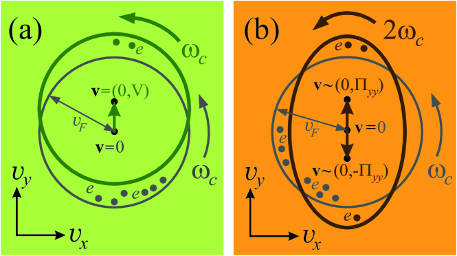
Figure 1: Schematic representation of the two distributions $f(\mathbf{v})$ of 2D electrons by their velocities $\mathbf{v}=(v_{x},v_{y})$. The equilibrium Fermi distributions $f_{F}(\mathbf{v})$ are shown by grey on both panels (a) and (b). The quasi-equilibrium distribution, $f_{\mathbf{V}}(\mathbf{v})=f_{F}(\mathbf{v}-\mathbf{V})$, with the mean hydrodynamic velocity $\mathbf{V}=(0,V)$ is shown by green at panel (a). In magnetic field such distribution function, together each individual electron, rotates with the frequency $\omega_{c}$. The nonequilibrium distribution, $f_{\Pi}(\mathbf{v})=f_{F}(\mathbf{v})+f_{2}(\mathbf{v})$, with zero mean velocity and the second harmonic $f_{2}(\mathbf{v})$ corresponding to a non-zero component $\Pi_{yy}$ of the momentum flux density tensor $\Pi_{ij}$ is shown by brown on panel (b). The rotation of individual electrons with the frequency $\omega_{c}$ leads to the rotation of such distribution function $f_{\Pi}$ with the frequency $2\omega_{c}$.

Second, we consider the case of a high-frequency flow when the characteristic frequencies $\omega$ are compared to $\omega_{c}$ and $1/\tau_{ee}$. As in the case of zero magnetic field, we decompose the values $\mathbf{V}(\mathbf{r},t)$ and $\Pi_{ij}(\mathbf{r},t)$ by the time harmonics proportional to $e^{-i\omega t}$. As a final result, we arrive to the Navier-Stocks equation for the amplitude $\mathbf{V}(\mathbf{r},\omega)$ of each velocity harmonic:

$$\begin{array}[]{c}\displaystyle-i\omega\mathbf{V}=\frac{e}{m}\mathbf{E}(\mathbf{r},\omega)+\omega_{c}\left[\mathbf{V}\times\mathbf{e}_{z}\right]-\frac{\mathbf{V}}{\tau}-\frac{\nabla P}{m}+\\ \\ \displaystyle+\eta_{xx}(\omega)\,\Delta\mathbf{V}+\eta_{xy}(\omega)\left[\Delta\mathbf{V}\times\mathbf{e}_{z}\right]\end{array}\>,$$ (9)

where the viscosity coefficients depend on magnetic field and frequency:

$$\begin{array}[]{c}\displaystyle\eta_{xx}(\omega)=\eta\frac{1-i\omega\tau_{ee}}{1+(-\omega^{2}+4\omega_{c}^{2})\tau_{ee}^{2}-2i\omega\tau_{ee}}\>,\\ \\ \displaystyle\eta_{xy}(\omega)=\eta\frac{2\omega_{c}\tau_{ee}}{1+(-\omega^{2}+4\omega_{c}^{2})\tau_{ee}^{2}-2i\omega\tau_{ee}}\>.\end{array}$$ (10)

It is seen that at $\omega_{c}\gg 1/\tau_{ee}$ the viscosity coefficients $\eta_{xx}(\omega)$ and $\eta_{xy}(\omega)$ exhibit a resonance at $\omega=2\omega_{c}$. Indeed, the own frequency of rotation of the value $\Pi_{ij}=m\langle v_{i}v_{j}\rangle$ is the doubled cyclotron frequency $2\omega_{c}$ (see Fig. 1). Thus when the frequency $\omega$ of variation of a flow is close to the internal frequency $2\omega_{c}$, the resonance occurs. It is not just a second harmonic of the one-particle cyclotron resonance, as it is related not to motion of individual electrons, but to the motion of the momentum flux of the electron ensemble (see Fig. 1). Such resonance is the special type of the high-order cyclotron resonance of collective electron motion related to the viscosity effect in magnetic field and so it can be called the viscous resonance.

If the interaction between 2D electrons is strong, they must be treated as a Fermi liquid. The Navier-Stocks equation (9), apparently, will describe flows of the fluid consisting of the quasiparticles of the Fermi liquid. The coefficients $\eta$ and $\zeta$ will contain the Landau parameters describing the interaction between quasiparticles. A preliminary analysis, following to Ref. zeta_F_zidk , shows that the conditions of applicability of the theory will expand significantly. In particular, the equations (9) and (10) will be applicable even at short wavelengths and high frequencies, $L\sim l_{\omega}$.

3. Plasmon damping. The time dispersion of viscosity can manifest itself in damping of the magnetoplasmons. Below we calculate the magnetoplasmon damping coefficient related to viscosity using the equations (4), (9), and (10). Herewith, we will not consider the retardation effects which can be important in the region of small wavevectors in some structures (see, for example, Ref. Falko_Khmelnitski ; Volkov_Zabolotnykh ).

For the case of waves in the absence of external ac fields, the electric field $\mathbf{E}(\mathbf{r},\omega)$ in Eq. (9) is induced by the perturbation of the 2D electron density $\delta n=n-n_{0}$. When we can neglect the retardation effects, we just have $\mathbf{E}=-\nabla\delta\varphi$, where $\delta\varphi$ is related to $\delta n$ by the electrostatic equations. For the structures with a metallic gate located at the distance $d$ from the 2D layer we have: $\delta\varphi=(4\pi ed/\kappa)\,\delta n$, where $\kappa$ is the background dielectric constant. For the structures without a gate the relation between $\delta\varphi(\mathbf{r},t)$ and $\delta n(\mathbf{r},t)$ is given just by the Coulomb law with the charge density $\varrho(\mathbf{r},z)=e\,\delta n(\mathbf{r})\,\delta(z)$, where $\delta(z)$ is the Delta-function depicting the position of the 2D layer.

We solve the together the equations (4), (9), and the electrostatic equation assuming that $\delta n(\mathbf{r},t)\,,\;\delta\varphi(\mathbf{r},t)\,,\;\mathbf{V}(\mathbf{r},t)\sim e^{-i\omega t+\mathbf{q}\cdot\mathbf{r}}$. The ratio of the terms $-\nabla P/m$ and $e\mathbf{E}/m$ in Eq. (9) is estimated as $a_{B}/d$ for the structures with a gate and as $a_{B}q$ for the ungated structures, where $a_{B}$ is the Bohr radius. Both these values must be much smaller than unity when the 2D electrostatic equations are applicable. Neglecting the terms describing the relaxation processes, we obtain from Eqs. (4) and (9) the usual formula for the dispersion law of magnetoplasmons. For the gated structures it is:

$$\omega_{0,q}=\sqrt{\omega_{c}^{2}+s^{2}q^{2}}$$ (11)

where $s=\sqrt{4\pi e^{2}n_{0}d/m\kappa}$. The second term under the root in Eq. (11), $s^{2}q^{2}$, is the squared plasmon frequency in the absence of magnetic field. For the ungated structure it changes on $2\pi e^{2}n_{0}q/m\kappa$.

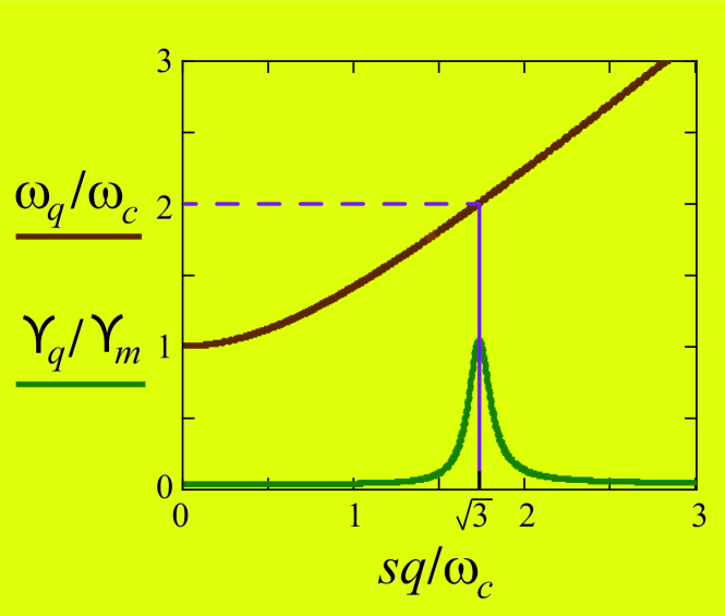
Figure 2: The magnetoplasmon dispersion law $\omega_{0,q}$ and the damping coefficient $\Upsilon_{q}$ calculated by Eqs. (11) and (14) for a gated structure. The maximum value of $\Upsilon_{q}$, $\Upsilon_{m}=5/(8\tau)+27\eta\omega_{c}^{2}/(8s^{2})$ is attained at the wavevector $q_{m}=\sqrt{3}\omega_{c}/s$ corresponding to the equality $\omega_{0,q}=2\omega_{c}$.

The viscosity terms and the terms describing scattering on disorder leads to a small correction to the magnetoplasmon dispersion (11) as well as to arising of a finite damping: $\omega_{q}=\omega_{0,q}+\Delta\omega_{q}-i\,\Upsilon_{q}$. The damping coefficient $\Upsilon_{q}$ takes the form:

$$\begin{array}[]{c}\displaystyle\Upsilon_{q}=\frac{\omega_{c}^{2}+\omega_{0,q}^{2}}{2\omega_{0,q}^{2}}\left[\frac{1}{\tau}+\mathrm{Re}\,\eta_{xx}q^{2}\right]+\frac{\omega_{c}}{\omega_{0,q}}\>\mathrm{Im}\,\eta_{xy}q^{2},\end{array}$$ (12)

Here the viscosity coefficients $\eta_{xx}(\omega)$ and $\eta_{xy}(\omega)$ are taken at $\omega=\omega_{0,q}$.

At high frequencies and high magnetic fields, $\omega,\omega_{c}\gg 1/\tau_{ee}$, we obtain from Eqs. (10) and (12):

$$\begin{array}[]{c}\displaystyle\Upsilon_{q}=\frac{1}{\tau}\frac{w^{2}+1}{2w^{2}}+\frac{\eta q^{2}}{w^{2}}\frac{w^{4}+13w^{2}+4}{4w^{2}+\beta^{2}(w^{2}-4)^{2}}\>,\end{array}$$ (13)

where $\beta=\omega_{c}\tau_{ee}\gg 1$ and $w=w(q)=\omega_{0,q}/\omega_{c}$. Near the resonance of the shear viscosity coefficients, when $w\approx 2$, the value $\Upsilon_{q}$ takes the form:

$$\Upsilon_{q}=\frac{5}{8\tau}+\frac{9\eta q^{2}}{8(1+\varepsilon^{2}\beta^{2})}\>.$$ (14)

where $\varepsilon=\varepsilon(q)=w(q)-2$, $\varepsilon\ll 1$. In high-quality structures at low temperature the inequality $1/\tau\lesssim\eta q^{2}/\beta^{2}$ can take place in certain intervals of wavevectors and magnetic fields. Provided this condition, the damping coefficient $\Upsilon_{q}$ in the resonance is greater than outside the resonance in $\beta^{2}\gg 1$ times [see Eq. (14) and Fig. 2].

4. Discussion and conclusion. In the case when a viscous flow of a 2D electron fluid is induced by an external ac electric field $\mathbf{E}_{ex}(\mathbf{r},t)\sim e^{-i\omega t}$, the viscosity effect, together with electron scattering on disorder, determines the absorbtion of energy from the external field. The linear response of a 2D fluid on $\mathbf{E}_{ex}(\mathbf{r},t)$ should be calculated from Eqs. (4) and (9). The resulting absorbtion coefficient will reflect the resonance dependence (14) of the magnetoplasmon damping, if the character plasmon wavelength $2\pi/q_{m}$ at the resonance frequency $\omega=2\omega_{c}$ is smaller that the sample width $W$.

It is possible that the viscous resonance is responsible also for the strong peak and features observed at $\omega=2\omega_{c}$ in the photoresistance exp_GaAs_ac_1 ; exp_GaAs_ac_2 and the photovoltaic effects exp_GaAs_ac_3 in the high-mobility GaAs quantum wells. Indeed, it was stressed in Ref. exp_GaAs_ac_1 that the strong peak in photovoltage and the very well pronounced giant negative magnetoresistance, explained in Ref. je_visc as a manifestation of forming of a viscous flow, are observed in the same best-quality GaAs structures. If a 2D electrons in such structures form a viscous fluid, than any response of the structure on ac field (absorbtion, photovoltage, photoresistance) must inevitably have peculiarities at the frequency of the viscous resonance.

To construct the theories of the photoresistance and the photovoltaic effects, one should supplement the hydrodynamic equation (9) by the nonlinear terms following to Refs. Lifshits_Dyakonov ; Beltukov_Dyakonov . The peak and features at $\omega=2\omega_{c}$ in photovoltage and photoresistance was observed in Refs. exp_GaAs_ac_1 ; exp_GaAs_ac_2 ; exp_GaAs_ac_3 at rather high magnetic fields when the inequality $R_{c}\ll W$ is fulfilled. A preliminary analysis shows that this justifies the applicability of the Fermi-gas model for the description of hydrodynamics near the viscous resonance. However, the Fermi-gas model outside the resonance, in particular, in small magnetic fields, seems to be irrelevant. Justification of the realization of hydrodynamics outside the resonance, possibly, within the Fermi-liquid model, requires further study.

To conclude, we predict the viscous resonance at $\omega=2\omega_{c}$ related to motion of the viscous stress tensor in magnetic field. This resonance manifest itself in the dependence of the damping of magnetoplasmons on their wavevectror and, probably, in the photoresistance and the photovoltaic effects.

The author wishes to thank Professor M. I. Dyakonov, under whose guidance this research was undertaken; for the discussions, advice, and support during the course of the work; and for his participation in writing the text of the Letter. The author also thanks A. P. Dmitriev and I. V. Gorniy for valuable discussions; D. G. Polyakov for attracting his attention to Ref. Kaufman ; A. P. Alekseeva, E. G. Alekseeva, I. P. Alekseeva, N. S. Averkiev, A. I. Chugunov, M. M. Glazov, I. V. Krainov, A. N. Poddubny, P. S. Shternin, D. S. Svinkin, and V. A. Volkov for advice and support. The part of this work devoted to the time dispersion of viscosity in magnetic field (Section 2) was supported by the Russian Science Foundation (Grant No. 17-12-01182); the part of this work devoted to plasmon damping due to viscosity (Section 3) was supported by the grant of the Basis Foundation.

References

- (1) R. N. Gurzhi, Sov. Phys. Uspekhi 94, 657 (1968).
- (2) V. L. Gurevich, Transport in Phonon Systems (Elsevier Science Publishers, Amsterdam - New York, 1986).
- (3) L. P. Pitaevskii, Sov. Phys. Uspekhi 11, 342 (1968).
- (4) P. J. W. Moll, P. Kushwaha, N. Nandi, B. Schmidt, and A. P. Mackenzie, Science 351, 1061 (2016).
- (5) J. Gooth, F. Menges, C. Shekhar, V. Suess, N. Kumar, Y. Sun, U. Drechsler, R. Zierold, C. Felser, and B. Gotsmann arXiv:1706.05925 (2017).
- (6) D. A. Bandurin, I. Torre, R. Krishna Kumar, M. Ben Shalom, A. Tomadin, A. Principi, G. H. Auton, E. Khestanova, K. S. NovoseIov, I. V. Grigorieva, L. A. Ponomarenko, A. K. Geim, and M. Polini, Science 351, 1055 (2016).
- (7) R. Krishna Kumar, D. A. Bandurin, F. M. D. Pellegrino, Y. Cao, A. Principi, H. Guo, G. H. Auton, M. Ben Shalom, L. A. Ponomarenko, G. Falkovich, K. Watanabe, T. Taniguchi, I. V. Grigorieva, L. S. Levitov, M. Polini, and A. K. Geim, Nature Physics DOI: 10.1038/NPHYS4240 (2017).
- (8) P. S. Alekseev, Phys. Rev. Lett. 117, 166601 (2016).
- (9) A. T. Hatke, M. A. Zudov, J. L. Reno, L. N. Pfeiffer, and K.W. West, Phys. Rev. B 85, 081304 (2012).
- (10) R. G. Mani, A. Kriisa, and W. Wegscheider, Scientific Reports 3, 2747 (2013).
- (11) L. Bockhorn, P. Barthold, D. Schuh, W. Wegscheider, and R. J. Haug, Phys. Rev. B 83, 113301 (2011).
- (12) Q. Shi, P. D. Martin, Q. A. Ebner, M. A. Zudov, L. N. Pfeiffer, and K. W. West, Phys. Rev. B 89, 201301 (2014).
- (13) R. N. Gurzhi, A. N. Kalinenko, and A. I. Kopeliovich, Phys. Rev. Lett. 74, 3872 (1995).
- (14) M. Hruska and B. Spivak, Phys. Rev. B 65, 033315 (2002).
- (15) A. V. Andreev, S. A. Kivelson, and B. Spivak, Phys. Rev. Lett. 106, 256804 (2011).
- (16) M. Mendoza, H. J. Herrmann, and S. Succi, Scientic reports 3, 1052 (2013).
- (17) A. Tomadin, G. Vignale, and M. Polini, Phys. Rev. Lett. 113, 235901 (2014).
- (18) L. Levitov and G. Falkovich, Nature Physics 12, 672 (2016); H. Guo, E. Ilseven, G. Falkovich, and L. Levitov, PNAS 114, 3068 (2017).
- (19) A. Lucas, Phys. Rev. B 95 115425 (2017); A. Lucas and K.C. Fong, arXiv: 1710.08425 (2017).
- (20) F. M. D. Pellegrino, I. Torre, and M. Polini, Phys. Rev. B 96, 195401 (2017).
- (21) P. S. Alekseev, A. P. Dmitriev, I. V. Gornyi, V. Y. Kachorovskii, B. N. Narozhny, M. Schutt, and M. Titov, Phys. Rev. Lett. 114, 156601 (2015).
- (22) G. Y. Vasileva, D. Smirnov, Y. L. Ivanov, Y. B. Vasilyev, P. S. Alekseev, A. P. Dmitriev, I. V. Gornyi, V. Y. Kachorovskii, M. Titov, B. N. Narozhny, R. J. Haug, Phys. Rev. B 93, 195430 (2016).
- (23) P. S. Alekseev, A. P. Dmitriev, I. V. Gornyi, V. Y. Kachorovskii, B. N. Narozhny, M. Schutt, and M. Titov, Phys. Rev. B 95, 165410 (2017).
- (24) P. S. Alekseev, A. P. Dmitriev, I. V. Gornyi, V. Y. Kachorovskii, M. A. Semina, Semiconductors 51, 766 (2017).
- (25) P. S. Alekseev, A. P. Dmitriev, I. V. Gornyi, V. Yu. Kachorovskii, B. N. Narozhny, and M. Titov Phys. Rev. B 97, 085109 (2018).
- (26) Se the website of the conferences devoted to the transport phenomena in the ultra-hign mobility 2D nanostructure: https://www.coulomb.univ-montp2.fr/MIRO-and-all-that?lang=en.
- (27) This work was reported at the seminar of the Institute of Nanotechnology (Karlsruhe Institute of Technology, Karlsruhe, Germany, 19 July 2017; for the abstract of the talk see https://www.int.kit.edu/calendar.php/event/33486) and at the Russian conference on semiconductor physics (Ekaterinburg, Russia, 2-6 October 2017; for the abstract of the talk see http://semicond2017.imp.uran.ru, p. 333; the deadline for abstract submission was 3 April 2017). The result similar to Eq. (10) was independengly obtained in Ref. eta_xy and published as the preprint arXiv:1706.08363 [cond-mat.mes-hall] on 26 June 2017 and as the article eta_xy on 1 November 2017. However, the existance of the resonance at was not noticed and discussed in that work.
- (28) Y. Dai, R. R. Du, L. N. Pfeiffer, and K. W. West, Phys. Rev. Lett. 105, 246802 (2010).
- (29) A. T. Hatke, M. A. Zudov, L. N. Pfeiffer, and K. W. West, Phys. Rev B 84, 241304 (2011).
- (30) M. Bialek, J. Lusakowski, M. Czapkiewicz, J. Wrobel, and V. Umansky, Phys. Rev B 91, 045437 (2015).
- (31) E. M. Lifshitz and L. P. Pitaevskii, Physical Kinetics (Pergamon Press, Oxford, 1981).
- (32) L. D. Landau and E. M. Lifshitz, Fluid Mechanics (Pergamon Press, Oxford, 1987).
- (33) M. S. Steinberg, Phys. Rev. 109, 1486 (1958).
- (34) Yu. M. Aliev, J. Appl. Mech. Tech. Phys. 3, 11 (1965).
- (35) A. N. Kaufman, Physics of Fluids 3, 610 (1960).
- (36) For the temperature dependence of the electron-phonon scattering rates in GaAs quantum wells see Refs. ph_rates_1 ; ph_rates_2 ; ph_rates_3 .
- (37) V. Karpus, Sov. Phys. Semicond. 20, 6 (1986).
- (38) P. S. Alekseev, M. S. Kipa, V. I. Perel, and I. N. Yassievich, JETP 106, 806 (2008).
- (39) M. S. Keepa, P. S. Alekseev, and I. N. Yassievich, Semiconductors 44, 198 (2010).
- (40) I. M. Khalatnikov and A. A. Abrikosov, Sov. Phys. JETP 6, 84 (1958).
- (41) In the second of Eq. (7) we assume that the electric field force is far smaller than the magnetic field force, as it usually takes place in the magnetotransport experiments.
- (42) V. I. Fal’ko and D. E. Khmel’nitskii, JETP 68, 1150 (1989).
- (43) V. A. Volkov and A. A. Zabolotnykh, Phys. Rev. B 89, 121410 (2014).
- (44) M. B. Lifshits and M. I. Dyakonov, Phys. Rev. B 80,121304 (2009).
- (45) Y. M. Beltukov and M. I. Dyakonov, Phys. Rev. Lett. 116, 176801 (2016).