Relationship between Magnetic Anisotropy Below Pseudogap Temperature and Short-Range Antiferromagnetic Order in High-Temperature Cuprate Superconductor

Abstract

The central issue in high-temperature cuprate superconductors is the pseudogap state appearing below the pseudogap temperature $T^{*}$, which is well above the superconducting transition temperature. In this study, we theoretically investigate the rapid increase of the magnetic anisotropy below the pseudogap temperature detected by the recent torque-magnetometry measurements on YBa₂Cu₃O_y [Y. Sato et al., Nat. Phys., 13, 1074 (2017)]. Applying the spin Green’s function formalism including the Dzyaloshinskii–Moriya interaction arising from the buckling of the CuO₂ plane, we obtain results that are in good agreement with the experiment and find a scaling relationship. Our analysis suggests that the characteristic temperature associated with the magnetic anisotropy, which coincides with $T^{*}$, is not a phase transition temperature but a crossover temperature associated with the short-range antiferromagnetic order.

The central issue in high-temperature cuprate superconductorsKeimer et al. (2015) is the nature and origin of the normal state pseudogap. Below the pseudogap temperature, $T^{*}$, which is higher than the superconducting transition temperature, $T_{c}$, a partial gap is observed in various experiments.Timusk and Statt (1999); Norman et al. (2005) The key question about the pseudogap is whether $T^{*}$ is a phase transition temperature or a crossover temperature. For instance, resonant ultrasound spectroscopy measurements exhibited a discontinuous change in the temperature dependence of frequency supporting that $T^{*}$ is the phase transition temperature.Shekhter et al. (2013) The measurement of the second–harmonic response, which detected the inversion symmetry breaking below $T^{*}$, also supported the phase transition picture.Zhao et al. (2016) Meanwhile, a phenomenological theory describing a crossover scenario was proposed,Yang et al. (2006); Rice et al. (2012) and spectroscopic and thermodynamic experiments were discussed using a model Green’s function with doping-dependent parameters. On the other hand, recent nuclear magnetic resonanceWu et al. (2011, 2013) and x-ray scatteringGhiringhelli et al. (2012); Achkar et al. (2012); Chang et al. (2012) studies reported a symmetry-breaking phase of the charge-density wave order in the pseudogap phase. Although the role of this order is unclear, it seems to compete with superconductivityKharkov and Sushkov (2016) and it appears at a temperature between $T^{*}$ and $T_{c}$. It has also been proposed that these orders are intertwined.Fradkin et al. (2015)

In this Letter, we focus on the recent torque-magnetometry measurements on YBa₂Cu₃O_y (YBCO) reporting a rapid increase in anisotropic spin susceptibility within the $a-b$ plane below $T^{*}$.Sato et al. (2017) A magnetic torque is induced if the magnetization ${\bm{M}}$ of the sample is not parallel to the applied magnetic field ${\bm{H}}$. When the magnetic field is rotated in the $x-y$ ($a-b$) plane by an azimuthal angle $\phi$, the magnetic torque is given by

$${\tau_{\phi}} = {\mu_{0}}V{\left({{\bm{M}}\times{\bm{H}}}\right)_{z}}$$ (1)

$$= \frac{1}{2}{\mu_{0}}V{H^{2}}\left[{\left({{\chi_{xx}}-{\chi_{yy}}}\right)\sin 2\phi-2{\chi_{xy}}\cos 2\phi}\right].$$

Here, $\mu_{0}$ is the permeability of vacuum and $V$ is the sample volume. The spin susceptibility is denoted by ${\chi_{\alpha\beta}}=\partial{M_{\alpha}}/\partial\left({{\mu_{0}}{H_{\beta}}}\right)$, with $\alpha,\beta=x,y$. For the CuO₂ plane with fourfold rotational symmetry, C₄, we see that $\tau_{\phi}=0$. In YBCO, ${\tau_{\phi}}$ exhibits sinusoidal oscillation with ${{\chi_{xx}}>{\chi_{yy}}}$ and $\chi_{xy}=0$.Sato et al. (2017) A rapid increase in the amplitude is observed below the characteristic temperature $T_{\tau}$ that coincides with the $T^{*}$ value determined by other experiments.Sato et al. (2017) The authors in Ref. Sato et al., 2017 conclude that $T_{\tau}$ corresponds to a nematic phase transition temperature and thus $T^{*}$ is also a phase transition temperature.

We propose a theory to explain this magnetic torque experiment. The theory is based on a localized spin model with anisotropic magnetic interaction. For this, we assume the Dzyaloshinskii–Moriya (DM) interactionBonesteel et al. (1992); Shekhtman et al. (1992); Koshibae et al. (1993) arising from the buckling of the CuO₂ plane. Usually, one may neglect this DM interaction owing to its energy scale. However, it breaks the C₄ symmetry and can play an important role for the physical quantities that do not vanish when the C₄ symmetry is broken. Applying second-order perturbation theory, we show that $\tau_{\phi}$ is proportional to cube of the spin susceptibility, and there is a scaling relationship. The analysis suggests that $T_{\tau}$ is the onset of a short-range antiferromagnetic (AF) order.

In describing the localized spins in the parent compound of the cuprate, the renormalization group analysis of the nonlinear $\sigma$ model was successful.Chakravarty et al. (1988) Mean field theories such as Schwinger bosonsArovas and Auerbach (1988) and modified spin wave theoryTakahashi (1989) also gave a good description of the system. However, these approaches are useful only in the low-temperature regime. At high temperatures around $T^{*}$, we need to take a different approach. Here, we take the spin Green’s function approach.Tyablikov and Bonch-Bruevich (1962); Kondo and Yamaji (1972); Shimahara and Takada (1991); Winterfeldt and Ihle (1997); Zavidonov and Brinkmann (1998); Sadovskii (2001)

For the calculation of $\tau_{\phi}$, we need to compute the following correlation functions:

$${\left\langle{S_{i}^{x}S_{j}^{x}}\right\rangle-\left\langle{S_{i}^{y}S_{j}^{y}}\right\rangle} = {{\mathop{\rm Re}\nolimits}\left\langle{S_{i}^{+}S_{j}^{+}}\right\rangle},$$ (2)

$${\left\langle{S_{i}^{x}S_{j}^{y}}\right\rangle+\left\langle{S_{i}^{y}S_{j}^{x}}\right\rangle} = {{\mathop{\rm Im}\nolimits}\left\langle{S_{i}^{+}S_{j}^{+}}\right\rangle}.$$ (3)

Here, $S_{j}^{\alpha}$ ($\alpha=x,y$) denotes the $\alpha$ component of the spin moment at site $j$. Note that these correlation functions depend on $i-j$ because of the translational invariance in the pseudogap phase. In the absence of any magnetically anisotropic term, the right-hand sides of these equations vanish. The Hamiltonian for the localized $S=1/2$ moments, on inclusion of the DM interaction mentioned above, is given by

$${\mathcal{H}}={J_{p}}\sum\limits_{\left\langle{i,j}\right\rangle}{{{\bm{S}}_{i}}\cdot{{\bm{S}}_{j}}}+\sum\limits_{\left\langle{i,j}\right\rangle}{{{\bm{D}}_{ij}}\cdot\left({{{\bm{S}}_{i}}\times{{\bm{S}}_{j}}}\right)}.$$ (4)

Here, $J_{p}$ is the exchange interaction between nearest-neighbor spins, which is assumed to depend on the doped hole concentration, $p$. The three-dimensional vector ${\bm{D}}_{ij}={\bm{D}}_{i-j}$ is the DM vector on the bond connecting sites $i$ and $j$. For the case of $D_{i-j}^{z}=0$, the DM interaction term is rewritten as

$${\mathcal{H}}_{{\rm{DM}}}=\sum\limits_{i}\sum\limits_{\delta=\widehat{a},\widehat{b}}{\left({{g_{\delta}}S_{i}^{-}S_{i+\delta}^{z}+H.c.}\right)}.$$ (5)

Here, $\widehat{a}$ and $\widehat{b}$ are the displacement vectors along the $a$ and $b$ axes, respectively, and ${g_{\delta}}=\left({iD_{\delta}^{x}-D_{\delta}^{y}}\right)/2$, with $D_{\delta}^{\alpha}$ being the $\alpha$ component of the DM vector. It is obvious from Eq. (5), that its first-order contribution to $\left\langle{S_{i}^{+}S_{j}^{+}}\right\rangle$ vanishes, but the second-order contribution does not.

Now, we define the following Matsubara Green’s function:

$${G_{i-j}}\left(\tau\right)=-\left\langle{{T_{\tau}}S_{i}^{+}\left(\tau\right)S_{j}^{-}\left(0\right)}\right\rangle,$$ (6)

with $\tau$ being the imaginary time. Taking the derivative of $G_{i-j}(\tau)$ with respect to $\tau$ twice, and then applying the Tyablikov approximation and the Fourier transform, we obtainKondo and Yamaji (1972); Shimahara and Takada (1991)

$$G_{\bm{k}}\left({i{\omega_{n}}}\right)=\frac{4J_{p}{c_{1}}\left(1-{\gamma_{\bm{k}}}\right)}{\left({i{\omega_{n}}}\right)^{2}-\omega_{\bm{k}}^{2}},$$ (7)

with $\omega_{n}$ denoting the Matsubara frequency and

$${c_{i-j}}=4\left\langle{S_{i}^{z}S_{j}^{z}}\right\rangle=2\left\langle{S_{i}^{+}S_{j}^{-}}\right\rangle=2\left\langle{S_{i}^{-}S_{j}^{+}}\right\rangle.$$ (8)

(Hereafter, we set $\hbar=1$ and the lattice constant is set to unity.) The spin excitation energy ${\omega_{\bm{k}}}$ is given by

$${\omega_{\bm{k}}}=\sqrt{8\alpha\left|{{c_{1}}}\right|}{J_{p}}\sqrt{\left({1-{\gamma_{\bm{k}}}}\right)\left({1+\Delta+{\gamma_{\bm{k}}}}\right)},$$ (9)

with ${\gamma_{\bm{k}}}=\left({\cos{k_{x}}+\cos{k_{y}}}\right)/2$ and $\Delta=\left({1-\alpha{c_{1}}+3\alpha{c^{\prime}_{2}}}\right)/\left({4\alpha\left|{{c_{1}}}\right|}\right)-1$. The parameter $\alpha$ is introduced while applying the Tyablikov approximation,Kondo and Yamaji (1972) which is interpreted as a vertex correction.Shimahara and Takada (1991) The parameter ${c^{\prime}_{2}}$ is defined by ${c^{\prime}_{2}}=\sum\limits_{\delta^{\prime}\left({\neq-\delta}\right)}{{c_{\delta+\delta^{\prime}}}}/3$. The parameters $c_{1}$, $\alpha$, and ${c^{\prime}_{2}}$ are determined by solving the following self-consistent equationsShimahara and Takada (1991):

$$1=-\frac{{4{J_{p}}{c_{1}}}}{N}\sum\limits_{\bm{k}}{\frac{{1-{\gamma_{\bm{k}}}}}{{{\omega_{\bm{k}}}}}\coth\left({\frac{{{\omega_{\bm{k}}}}}{2k_{B}T}}\right)},$$ (10)

$${c_{1}}=-\frac{{4{J_{p}}{c_{1}}}}{N}\sum\limits_{\bm{k}}{\frac{{{\gamma_{\bm{k}}}\left({1-{\gamma_{\bm{k}}}}\right)}}{{{\omega_{\bm{k}}}}}\coth\left({\frac{{{\omega_{\bm{k}}}}}{2k_{B}T}}\right)},$$ (11)

$$\frac{{3{c^{\prime}_{2}}+1}}{4}=-\frac{{4{J_{p}}{c_{1}}}}{N}\sum\limits_{\bm{k}}{\frac{{\gamma_{\bm{k}}^{2}\left({1-{\gamma_{\bm{k}}}}\right)}}{{{\omega_{\bm{k}}}}}\coth\left({\frac{{{\omega_{\bm{k}}}}}{2k_{B}T}}\right)}.$$ (12)

Here, $N$ is the number of the lattice sites, and $k_{B}$ is the Boltzmann constant.

The second-order perturbative calculation with respect to $H_{DM}$ gives

$$\left\langle{S_{i}^{+}S_{j}^{+}}\right\rangle = \frac{{{k_{\rm{B}}}T}}{{2N}}\sum\limits_{\bm{k}}{\sum\limits_{\delta,\delta^{\prime}}{{g_{\delta}}{g_{\delta^{\prime}}}{e^{i{\bm{k}}\cdot\left({\delta-\delta^{\prime}}\right)}}}\sum\limits_{i{\omega_{n}}}{{e^{i{\bm{k}}\cdot\left({{{\bm{R}}_{i}}-{{\bm{R}}_{j}}}\right)}}}}$$ (13)

$$\times{G_{\bm{k}}}\left({i{\omega_{n}}}\right){G_{-{\bm{k}}}}\left({-i{\omega_{n}}}\right){G_{-{\bm{k}}}}\left({i{\omega_{n}}}\right),$$

where $\bm{R}_{i}$ denotes the position of site $i$. The summation over $i$ shows that we need only the ${\bm{k}}=0$ term. The terms with $\omega_{n}\neq 0$ vanish if we set ${\bm{k}}=0$. Therefore, we may set $\omega_{n}=0$, and then ${\bm{k}}=0$. The result is

$$\frac{1}{N}\sum\limits_{i}{\left\langle{S_{i}^{+}S_{j}^{+}}\right\rangle}=\frac{{{k_{\rm{B}}}T}}{{16J_{p}^{3}{\alpha^{3}}{{\left({2+\Delta}\right)}^{3}}}}\Gamma,$$ (14)

with $\Gamma={\left({{g_{\widehat{a}}}+{g_{\widehat{b}}}}\right)^{2}}$. By using this result, we obtain

$$\Delta{\chi}\equiv\frac{{{\tau_{\phi}}}}{{{\mu_{0}}V{H^{2}}/2}}=\frac{{{\mu_{0}}\mu_{B}^{2}}}{{2{v_{c}}}}\frac{{{\Gamma_{\parallel}}\sin 2\phi-{\Gamma_{\bot}}\cos 2\phi}}{{J_{p}^{3}{\alpha^{3}}{{\left({2+\Delta}\right)}^{3}}}},$$ (15)

where ${v_{c}}$ is the unit cell volume per CuO₂ plane, and ${\Gamma_{\parallel}}={\mathop{\rm Re}\nolimits}\Gamma$ and ${\Gamma_{\bot}}={\mathop{\rm Im}\nolimits}\Gamma$. $\Delta{\chi}$ oscillates with two components: one is proportional to $\sin 2\phi$, and the other is proportional to $\cos 2\phi$. We note thatShimahara and Takada (1991)

$$\frac{1}{N}\sum\limits_{i}{\left\langle{S_{i}^{+}S_{j}^{-}}\right\rangle}=\frac{1}{{2{J_{p}}\alpha\left({2+\Delta}\right)}}.$$ (16)

Therefore, the right-hand side of Eq. (15) is proportional to the cube of the spin susceptibility.

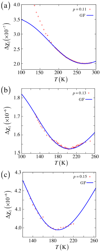
Now we apply the theory to the experiment.Sato et al. (2017) For YBCO, $D_{\widehat{a}}^{y}\neq 0$, $D_{\widehat{b}}^{x}\neq 0$, and the other components are negligible.Bonesteel (1993) Thus, ${\Gamma_{\parallel}}\neq 0$ and ${\Gamma_{\bot}}=-\left[{D_{a}^{\left(x\right)}D_{a}^{\left(y\right)}+D_{b}^{\left(x\right)}D_{b}^{\left(y\right)}}\right]/2=0$. Therefore, we find $\tau_{\phi}\propto\sin 2\phi$, which is the oscillation pattern observed in the experiment.Sato et al. (2017) Hereafter, we consider the case $\Gamma_{\bot}=0$, and denote $\Delta\chi$ as $\Delta\chi_{\parallel}$. The theoretical formula (15) is compared with the experimentSato et al. (2017) with the fitting parameters $J_{p}$ and ${\Gamma_{\parallel}}$ by including a constant term consisting of a temperature-independent paramagnetic component. The results shown in Fig. 1 demonstrate that the theory is in good agreement with the experiment. From the fitting, we found $J_{0.11}=241$ K, $J_{0.13}=183$ K, and $J_{0.15}=170$ K as the values of $J_{p}$ for $p$ = 0.11, 0.13, and 0.15 respectively. The value of $J_{p}$ decreases as $p$ is increased. This monotonic change in $J_{p}$ as a function of $p$ was also suggested from an analysis of the spin susceptibility and a scaling was found in La_2-xSr_xCuO_4-y.Johnston (1989); Nakano et al. (1994) For $p=0.11$, there is a discrepancy between theory and the experiment at low temperatures. This is because the spin Green’s function approach is not reliable at low temperatures.Shimahara and Takada (1991) We note that this discrepancy starts from $0.40J_{p}$ below the minimum of $\Delta\chi_{\parallel}$. The data for $p=0.13$ and $p=0.15$ are well above this value.

Figure 1: (color online) Comparisons between the formula (15) and the experimentsSato et al. (2017) for hole concentrations (a) $p=0.11$, (b) $p=0.13$, and (c) $p=0.15$. The solid lines represent the theory based on the spin Green’s function.

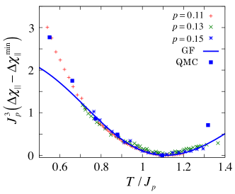
From the formula (15), we see that $J_{p}^{3}\Delta{\chi_{\parallel}}$ is independent of $J_{p}$. In order to remove constant components coming from doped holes, we subtract its minimum value from $\Delta{\chi_{\parallel}}$, and then plot it as a function of the normalized temperature in Fig. 2. All the experimental data fall on a single curve. From this analysis, we may conclude that $T_{\tau}\simeq 1.1J_{p}$. This characteristic temperature has a simple interpretation. The AF correlation length of the AF Heisenberg model with the exchange interaction $J_{p}$ is given byTakahashi (1989)

$${\xi_{{\rm{AF}}}/a}\simeq\frac{{0.819}}{{T/{J_{p}}}}\exp\left({\frac{{1.10}}{{T/{J_{p}}}}}\right),$$ (17)

where $a$ is the lattice constant. From this formula, we find $\xi_{\rm AF}\simeq 2a$ at $T=T_{\tau}$. In Fig. 2 we also plot the values computed using quantum Monte Carlo (QMC) results for the uniform spin susceptibility $\chi$ on the square lattice AF Heisenberg model.Okabe and Kikuchi (1988) These values are in good agreement with the data of $p=0.11$ at low temperatures. However, the point computed from the QMC data around $T/J_{p}=1.3$ does not agree with the experiment and the Green’s function result. We note that we find ${\Gamma_{\parallel}}<0$ from the fact that the magnitude of the DM vector is proportional to the difference in the lattice constants in the orthorhombic phase of YBCO. This is consistent with the experiment because the maximum of $\chi$ corresponds to the minimum of $\Delta{\chi_{\parallel}}$. We also note that the experimental data seem to be convex upward for $T>T_{\tau}$ at $p=0.13$ and $p=0.15$. However, a similar behavior is not discernible for $p=0.11$. It might be related to the effect of doped holes and/or CuO chains.

Figure 2: (color online) Scaling relationship suggested from the formula (15). $\Delta\chi_{\parallel}^{\min}$ is the minimum of $\Delta\chi_{\parallel}$ in Fig. 1. The unit of the vertical axis is K³. For the values of $J_{p}$, we take $J_{0.11}=241$ K, $J_{0.13}=183$ K, and $J_{0.15}=170$ K for the experimental data. The values computed by using QMC resultOkabe and Kikuchi (1988) are also shown.

Now we discuss the value of $\Gamma_{\parallel}$. From the analysis shown in Fig. 2, we find $\sqrt{|\Gamma_{\parallel}|}\simeq 100$ K. This apparently is too large if $\Gamma_{\parallel}$ is associated with the buckling of the CuO₂ plane. Here, we need to include the effect of the doped holes. The exchange coupling between doped hole spins and the localized spins is described by ${\mathcal{H}}_{K}={J_{K}}\sum\limits_{j}{{{\bm{S}}_{j}}\cdot\left({c_{j}^{\dagger}{\bm{\sigma}}{c_{j}}}\right)}$, where ${J_{K}}=t_{dp}^{2}/\left({{U_{d}}-\Delta}\right)+t_{dp}^{2}/\left({{U_{p}}+\Delta}\right)$, where $t_{dp}$ is the nearest-neighbor Cu-O hopping and $U_{d}$ ($U_{p}$) is the Cu(O)-site Coulomb repulsion.Zhang and Rice (1988); Tohyama and Maekawa (1990); Matsukawa and Fukuyama (1989) $\Delta$ is the energy difference between the O-site energy and the Cu-site energy. The two-component operator $c_{j}^{\dagger}$ ($c_{j}$) is the creation (annihilation) operator of the doped hole at site $j$, and ${\bm{\sigma}}$ is the three component vector of the Pauli matrices. The easiest way to include ${\mathcal{H}}_{K}$ is the coherent state path integral. By integrating out the doped hole fields, we find that the spin susceptibility $\chi$ is enhanced as $\chi/\left({1-\eta\chi}\right)$ with $\eta=3J_{K}^{2}\chi_{0}^{\rm{h}}$. Here, $\chi_{0}^{\rm{h}}$ is the uniform spin susceptibility of the doped holes. Unfortunately no reliable theoretical formula for $\chi_{0}^{\rm{h}}$ is available. Therefore, we use the formula for the non-interacting system, which is proportional to the density of states, and approximate it as $\chi_{0}^{\rm{h}}\sim 1/t$ where $t\sim t_{dp}^{2}/\Delta$ is the effective hopping parameter of the doped holes.Zhang and Rice (1988); Tohyama and Maekawa (1990); Matsukawa and Fukuyama (1989) Using the parameter values evaluated for the CuO₂ plane,Tohyama and Maekawa (1990); Eskes et al. (1989); Hybertsen et al. (1990); Matsukawa and Fukuyama (1989) we find that $\eta/J_{p}\sim 10$. With this value of $\eta/J_{p}$, $\sqrt{|\Gamma_{\parallel}|}\sim 2$ K. For $\eta/J_{p}=9$, $\sqrt{|\Gamma_{\parallel}|}\sim 15$ K. Although this is an approximate estimate, these values appear to be reasonable from the fact that $\Gamma_{\parallel}$ is proportional to the difference between the lattice constants along the $a$ and $b$ axes and also the buckling angle.

To conclude, we have shown that the result of the theory based on the spin Green’s function with the DM interaction is in good agreement with the recent torque-magnetometry measurements of YBCO.Sato et al. (2017) There is a clear scaling relationship as shown in Fig. 2. Our analysis shows that the magnetic anisotropy increases rapidly below $T_{\tau}\simeq 1.1J_{p}$ at which $\xi_{\rm AF}\simeq 2a$. Therefore, $T_{\tau}$ is a crossover temperature associated with the short-range AF order, in contrast to the claim in Ref. Sato et al., 2017 where $T_{\tau}$ is interpreted as an onset of a nematic phase transition. Given the experimental fact that $T_{\tau}$ coincides with the onset temperature of the pseudogap, the pseudogap may also be a crossover phenomenon.

References

- Keimer et al. (2015) B. Keimer, S. Kivelson, M. Norman, S. Uchida, and J. Zaanen, Nature, 518, 179 (2015).
- Timusk and Statt (1999) T. Timusk and B. W. Statt, Rep. Prog. Phys., 62, 61 (1999).
- Norman et al. (2005) M. R. Norman, D. Pines, and C. Kallin, Adv. Phys., 54, 715 (2005).
- Shekhter et al. (2013) A. Shekhter, B. J. Ramshaw, R. Liang, W. N. Hardy, D. A. Bonn, F. F. Balakirev, R. D. McDonald, J. B. Betts, S. C. Riggs, and A. Migliori, Nature, 498, 75 (2013).
- Zhao et al. (2016) L. Zhao, C. A. Belvin, R. Liang, D. A. Bonn, W. N. Hardy, N. P. Armitage, and D. Hsieh, Nat. Phys., 13, 250 (2016).
- Yang et al. (2006) K.-Y. Yang, T. M. Rice, and F.-C. Zhang, Phys. Rev. B, 73, 174501 (2006).
- Rice et al. (2012) T. M. Rice, K.-Y. Yang, and F. C. Zhang, Rep. Prog. Phys., 75, 016502 (2012).
- Wu et al. (2011) T. Wu, H. Mayaffre, S. Krämer, M. Horvatić, C. Berthier, W. N. Hardy, R. Liang, D. A. Bonn, and M.-H. Julien, Nature, 477, 191 (2011).
- Wu et al. (2013) T. Wu, H. Mayaffre, S. Krämer, M. Horvatić, C. Berthier, P. L. Kuhns, A. P. Reyes, R. Liang, W. N. Hardy, D. A. Bonn, and M.-H. Julien, Nat. Commun., 4 (2013), doi:10.1038/ncomms3113.
- Ghiringhelli et al. (2012) G. Ghiringhelli, M. L. Tacon, M. Minola, S. Blanco-Canosa, C. Mazzoli, N. B. Brookes, G. M. D. Luca, A. Frano, D. G. Hawthorn, F. He, T. Loew, M. M. Sala, D. C. Peets, M. Salluzzo, E. Schierle, R. Sutarto, G. A. Sawatzky, E. Weschke, B. Keimer, and L. Braicovich, Science, 337, 821 (2012).
- Achkar et al. (2012) A. J. Achkar, R. Sutarto, X. Mao, F. He, A. Frano, S. Blanco-Canosa, M. L. Tacon, G. Ghiringhelli, L. Braicovich, M. Minola, M. M. Sala, C. Mazzoli, R. Liang, D. A. Bonn, W. N. Hardy, B. Keimer, G. A. Sawatzky, and D. G. Hawthorn, Phys. Rev. Lett., 109 (2012), doi:10.1103/physrevlett.109.167001.
- Chang et al. (2012) J. Chang, E. Blackburn, A. T. Holmes, N. B. Christensen, J. Larsen, J. Mesot, R. Liang, D. A. Bonn, W. N. Hardy, A. Watenphul, M. v. Zimmermann, E. M. Forgan, and S. M. Hayden, Nat. Phys., 8, 871 (2012).
- Kharkov and Sushkov (2016) Y. A. Kharkov and O. P. Sushkov, Sci. Rep., 6 (2016), doi:10.1038/srep34551.
- Fradkin et al. (2015) E. Fradkin, S. A. Kivelson, and J. M. Tranquada, Rev. Mod. Phys., 87, 457 (2015).
- Sato et al. (2017) Y. Sato, S. Kasahara, H. Murayama, Y. Kasahara, E.-G. Moon, T. Nishizaki, T. Loew, J. Porras, B. Keimer, T. Shibauchi, and Y. Matsuda, Nat. Phys., 13, 1074 (2017).
- Bonesteel et al. (1992) N. E. Bonesteel, T. M. Rice, and F. C. Zhang, Phys. Rev. Lett., 68, 2684 (1992).
- Shekhtman et al. (1992) L. Shekhtman, O. Entin-Wohlman, and A. Aharony, Phys. Rev. Lett., 69, 836 (1992).
- Koshibae et al. (1993) W. Koshibae, Y. Ohta, and S. Maekawa, Phys. Rev. B, 47, 3391 (1993).
- Chakravarty et al. (1988) S. Chakravarty, B. I. Halperin, and D. R. Nelson, Phys. Rev. Lett., 60, 1057 (1988).
- Arovas and Auerbach (1988) D. P. Arovas and A. Auerbach, Phys. Rev. B, 38, 316 (1988).
- Takahashi (1989) M. Takahashi, Phys Rev B, 40, 2494 (1989).
- Tyablikov and Bonch-Bruevich (1962) S. Tyablikov and V. Bonch-Bruevich, Adv. Phys., 11, 317 (1962).
- Kondo and Yamaji (1972) J. Kondo and K. Yamaji, Progr. Theoret. Phys., 47, 807 (1972).
- Shimahara and Takada (1991) H. Shimahara and S. Takada, J. Phys. Soc. Jpn., 60, 2394 (1991).
- Winterfeldt and Ihle (1997) S. Winterfeldt and D. Ihle, Phys. Rev. B, 56, 5535 (1997).
- Zavidonov and Brinkmann (1998) A. Y. Zavidonov and D. Brinkmann, Phys. Rev. B, 58, 12486 (1998).
- Sadovskii (2001) M. V. Sadovskii, Phys. Usp., 44, 515 (2001).
- Bonesteel (1993) N. E. Bonesteel, Phys. Rev. B, 47, 11302 (1993).
- Johnston (1989) D. C. Johnston, Phys. Rev. Lett., 62, 957 (1989).
- Nakano et al. (1994) T. Nakano, M. Oda, C. Manabe, N. Momono, Y. Miura, and M. Ido, Phys. Rev. B, 49, 16000 (1994).
- Okabe and Kikuchi (1988) Y. Okabe and M. Kikuchi, J. Phys. Soc. Jpn., 57, 4351 (1988).
- Zhang and Rice (1988) F. C. Zhang and T. M. Rice, Phys. Rev. B, 37, 3759 (1988).
- Tohyama and Maekawa (1990) T. Tohyama and S. Maekawa, J. Phys. Soc. Jpn., 59, 1760 (1990).
- Matsukawa and Fukuyama (1989) H. Matsukawa and H. Fukuyama, J. Phys. Soc. Jpn., 58, 2845 (1989).
- Eskes et al. (1989) H. Eskes, G. Sawatzky, and L. Feiner, Physica C, 160, 424 (1989).
- Hybertsen et al. (1990) M. S. Hybertsen, E. B. Stechel, M. Schluter, and D. R. Jennison, Phys. Rev. B, 41, 11068 (1990).