Growth of periodic Grigorchuk groups

Abstract.

On torsion Grigorchuk groups we construct random walks of finite entropy and power-law tail decay with non-trivial Poisson boundary. Such random walks provide near optimal volume lower estimates for these groups. In particular, for the first Grigorchuk group $G$ we show that its growth $v_{G,S}(n)$ satisfies $\lim_{n\to\infty}\log\log v_{G,S}(n)/\log n=\alpha_{0}$, where $\alpha_{0}=\frac{\log 2}{\log\lambda_{0}}\approx 0.7674$, $\lambda_{0}$ is the positive root of the polynomial $X^{3}-X^{2}-2X-4$.

1. Introduction

Let $\Gamma$ be a finitely generated group and $S$ be a finite generating set of $\Gamma$. The word length $l_{S}(\gamma)$ of an element $\gamma\in\Gamma$ is the smallest integer $n\geq 0$ for which there exists $s_{1},\ldots,s_{n}\in S\cup S^{-1}$ such that $\gamma=s_{1}\ldots s_{n}$. The growth function $v_{\Gamma,S}(n)$ counts the number of elements with word length $l_{S}(\gamma)\leq n$, that is

$$v_{\Gamma,S}(n)=\#\{\gamma\in\Gamma:\ l_{S}(\gamma)\leq n\}.$$

A finitely generated group $\Gamma$ is of polynomial growth if there exists $0<D<\infty$ and a constant $C>0$ such that $v_{\Gamma,S}(n)\leq Cn^{D}$. It is of exponential growth if there exists $\lambda>1$ and $c>0$ such that $v_{\Gamma,S}(n)\geq c\lambda^{n}$. If $v_{\Gamma,S}(n)$ is sub-exponential but $\Gamma$ is not of polynomial growth, we say $\Gamma$ is a group of intermediate growth. Any group of polynomial growth is virtually nilpotent by Gromov’s theorem [gromov]. For some classes of groups the growth is either polynomial or exponential (for example, for solvable groups by results of Milnor and Wolf [Milnor], [Wolf], and for linear groups as it follows from Tits alternative [Tits]). The first examples of groups of intermediate growth are constructed by Grigorchuk in [Grigorchuk84].

Grigorchuk groups are indexed by infinite strings $\omega$ in $\{{\bf 0},{\bf 1},{\bf 2}\}^{\infty}$ (whose definitions are recalled in Subsection 2.4). Following [Grigorchuk84], for any such $\omega$, we associate automorphisms $a,b_{\omega},c_{\omega},d_{\omega}$ of the rooted binary tree. Consider the group $G_{\omega}$ generated by $S=\{a,b_{\omega},c_{\omega},d_{\omega}\}$. For the string $\omega=({\bf 012})^{\infty}$, the corresponding group is called the first Grigorchuk group, which was introduced in Grigorchuk [Grigorchuk80]. By [Grigorchuk84], if $\omega$ is eventually constant then $G_{\omega}$ is virtually abelian (hence of polynomial growth); otherwise $G_{\omega}$ is of intermediate growth. The group $G_{\omega}$ is periodic (also called torsion) if and only if $\omega$ contains all three letters ${\bf 0},{\bf 1},{\bf 2}$ infinitely often.

A long-standing open question, since the construction of Grigorchuk groups of intermediate growth in [Grigorchuk84], is to find the asymptotics of their growth functions. Among them the first Grigorchuk group $G=G_{012}$ has been the most investigated. In Grigorchuk [Grigorchuk84], it was shown that

$$\exp(cn^{1/2})\leq v_{G,S}(n)\leq\exp\left(Cn^{\beta}\right),$$

where $\beta=\log_{32}31$. The upper bound above which shows that $G$ is of sub-exponential growth is based on norm contracting property. The property considered in [Grigorchuk84] is as follows. There is an integer $d\geq 2$ and an injective homomorphism $\psi=(\psi_{i})_{i=1}^{d}$ from a finite index subgroup $H$ of $G$ into $G^{d}$ such that for any $h\in H$, with respect to word length $\left|\cdot\right|=l_{S}$ on $G$,

(1.1) $$\sum_{i=1}^{d}\left|\psi_{i}(h)\right|\leq\eta|h|+C$$

for some constant $C>0$ and contraction coefficient $\eta\in(0,1)$. Later Bartholdi in [Bartholdi98] has shown that there exist choices of norm that achieve better contraction coefficient than the word length $l_{S}$, and therefore a better upper bound for growth; in [MuchnikPak] Muchnik and Pak show similar growth upper bounds for more general $\omega$ including $({\bf 012})^{\infty}$ and for further generalizations of $G_{\omega}$. The upper bound in [Bartholdi98, MuchnikPak] states that

$$v_{G,S}(n)\leq\exp\left(Cn^{\alpha_{0}}\right),$$

where $\alpha_{0}=\frac{\log 2}{\log\lambda_{0}}\approx 0.7674$, where $\lambda_{0}$ is the positive root of the polynomial $X^{3}-X^{2}-2X-4$.

The lower bound $e^{n^{1/2}}$ proved by Grigorchuk uses what he calls anti-contraction properties on $G$. It remained open whether $v_{G,S}$ grows strictly faster than $e^{n^{1/2}}$ until Leonov [Leonov] introduced an algorithm which led to a better anti-contraction coefficient and showed that $v_{G,S}(n)\geq\exp\left(cn^{0.504}\right)$. Bartholdi [Bartholdi01] obtained that $v_{G,S}(n)\geq\exp\left(cn^{0.5157}\right)$. In the thesis of Brieussel [brieussel], Corollary 1.4.2 states that $v_{G,S}(n)\geq\exp\left(cn^{0.5207}\right)$.

Let $\mu$ be a probability measure on a group $\Gamma$. A function $f:\Gamma\to\mathbb{R}$ is $\mu$-harmonic if $f(x)=\sum_{y\in G}f(xy)\mu(y)$ for all $x\in\Gamma$. Among several definitions of the Poisson boundary of $(\Gamma,\mu)$, also called the Poisson-Furstenberg boundary, one is formulated in terms of the measure theoretic boundary that represents all bounded $\mu$-harmonic functions on $\Gamma$, see [KV83]. In particular the Poisson boundary of $(\Gamma,\mu)$ is trivial if and only if all bounded $\mu$-harmonic functions on $\Gamma$ are constant. The (Shannon) entropy of a measure $\mu$ is defined as $H(\mu)=-\sum_{g\in\Gamma}\mu(g)\log\mu(g)$. When $\Gamma$ is finitely generated, the entropy criterion of Kaimanovich-Vershik [KV83] and Derriennic [derriennic] provides a quantitative relation between the growth function of $\Gamma$ and the tail decay of a measure $\mu$ of finite entropy and non-trivial Poisson boundary on $\Gamma$, see more details reviewed in Subsection 2.1.

In this paper we construct probability measures with non-trivial Poisson boundary on torsion Grigorchuk groups. The measures are chosen to have finite entropy and explicit control over their tail decay, that is, with an upper bound on $\mu\left(\left\{g:l_{S}(g)\geq n\right\}\right).$ The main contribution of the paper is that on a collection of Grigorchuk groups, including these indexed by periodic strings containing three letters ${\bf 0},{\bf 1},{\bf 2}$, we construct such measures with good tail decay that provide near optimal volume lower estimates. Our main result Theorem 8.3 specialized to the first Grigorchuk group $G_{012}$ is the following.

Theorem A.

Let $\alpha_{0}=\frac{\log 2}{\log\lambda_{0}}\approx 0.7674$, where $\lambda_{0}$ is the positive root of the polynomial $X^{3}-X^{2}-2X-4$. For any $\epsilon>0$, there exists a constant $C_{\epsilon}>0$ and a non-degenerate symmetric probability measure $\mu$ on $G=G_{012}$ of finite entropy and nontrivial Poisson boundary, where the tail decay of $\mu$ satisfies that for all $r\geq 1$,

$$\mu\left(\left\{g:l_{S}(g)\geq r\right\}\right)\leq C_{\epsilon}r^{-\alpha_{0}+\epsilon}.$$

As a consequence, for any $\epsilon>0$, there exists a constant $c_{\epsilon}>0$ such that for all $n\geq 1$,

$$v_{G,S}(n)\geq\exp\left(c_{\epsilon}n^{\alpha_{0}-\epsilon}\right).$$

We construct measures of non-trivial Poisson boundary needed for the proof of Theorem A by introducing and studying some asymptotic invariants of the group, related to the diameter and shape of what we call "quasi-cubic sets" and "uniformised quasi-cubic sets" (see Subsection 1.1 where we sketch the proof). The main problem we address is how to use the geometric and algebraic structure of the groups to construct measures with good control over the tail decay such that careful analysis of the induced random walks on the Schreier graph can be performed to show non-triviality of the Poisson boundary.

The volume lower bound in Theorem A matches up in exponent with Bartholdi’s upper bound in [Bartholdi98]. In particular, combined with the upper bound we conclude that the volume exponent of the first Grigorchuk group $G$ exists and is equal to $\alpha_{0}$, that is

$$\lim_{n\to\infty}\frac{\log\log v_{G,S}(n)}{\log n}=\alpha_{0}.$$

It was open whether the limit exists. Our argument applies to a large class of $\omega$ satisfying certain assumptions, see Theorem 8.3. In particular the assumption of the theorem is verified by all periodic strings containing $3$ letters ${\bf 0},{\bf 1},{\bf 2}$, or strings that are products of ${\bf 201}$ and ${\bf 211}.$ For general $\omega$, volume upper bounds on $G_{\omega}$ are based on the norm contracting property (1.1) first shown in Grigorchuk [Grigorchuk84], and suitable choices of norms are given in the work of Muchnik and Pak [MuchnikPak], Bartholdi and the first named author [BE2]. Combining with upper bounds from [BE2], we derive the following two corollaries from Theorem 8.3.

For a periodic string $\omega$ that contains all three letters ${\bf 0},{\bf 1},{\bf 2}$, we show that the volume exponent of $G_{\omega}$ exists. Let $M_{i}$, $i\in\{{\bf 0},{\bf 1},{\bf 2}\}$, be matrices defined as

$$M_{{\bf 0}}=\left[\begin{array}[]{ccc}2&0&1\\ 0&2&1\\ 0&0&1\end{array}\right],M_{{\bf 1}}=\left[\begin{array}[]{ccc}2&1&0\\ 0&1&0\\ 0&1&2\end{array}\right],M_{{\bf 2}}=\left[\begin{array}[]{ccc}1&0&0\\ 1&2&0\\ 1&0&2\end{array}\right].$$

Theorem B.

Let $\omega\in\{{\bf 0},{\bf 1},{\bf 2}\}^{\infty}$ be a periodic string $\omega=(\omega_{0}\ldots\omega_{q-1})^{\infty}$ of period $q$ which contains all three letters ${\bf 0},{\bf 1},{\bf 2}$. Then the growth exponent of the Grigorchuk group $G_{\omega}$ exists and

$$\lim_{n\to\infty}\frac{\log\log v_{G_{\omega},S}(n)}{\log n}=\alpha_{\omega},$$

where $\alpha_{\omega}=\frac{q\log 2}{\log\lambda}$ and $\lambda=\lambda_{\omega_{0}\ldots\omega_{q-1}}$ is the spectral radius of the matrix $M_{\omega_{0}}\ldots M_{\omega_{q-1}}$.

By [Grigorchuk84, Theorem 7.2] the family $\{G_{\omega}\}$ provides a continuum of mutually non-equivalent growth functions. When $\omega$ is not periodic, Grigorchuk shows in [Grigorchuk84] that for some choices of $\omega$, the growth of $G_{\omega}$ exhibits oscillating behavior: $\lim_{n\to\infty}\log\log v_{G_{\omega}}(n)/\log n$ does not exist. Together with upper bounds from [BE2], our lower bounds show that given numbers $\alpha\leq\beta$ in $[\alpha_{0},1]$, there exists a $G_{\omega}$ which realizes these prescribed numbers as lower and upper volume exponents.

Theorem C.

For any $\alpha,\beta$ such that $\alpha_{0}\leq\alpha\leq\beta\leq 1$, where $\alpha_{0}\approx 0.7674$ is the volume exponent of $G_{012}$, there exists $\omega\in\{{\bf 0},{\bf 1},{\bf 2}\}^{\infty}$ such that the Grigorchuk group $G_{\omega}$ satisfies

$$\liminf_{n\to\infty}\frac{\log\log v_{G_{\omega},S}(n)}{\log n} =\alpha,$$

$$\limsup_{n\to\infty}\frac{\log\log v_{G_{\omega},S}(n)}{\log n} =\beta.$$

Theorem C is a special case of the more precise statement in Theorem 8.5. We mention that for some groups of intermediate growth there is no way to obtain a near optimal lower bound of the growth function using tail decay of measures of non-trivial Poisson boundary. For instance, there are extensions of the first Grigorchuk group that are of intermediate growth, where the growth function can be arbitrarily close to exponential but any random walk with finite $\alpha_{0}$-moment has trivial Poisson boundary, see Remark 9.3 at the end of the paper.

1.1. Sketch of the arguments for the first Grigorchuk group

For a nilpotent group $\Gamma$ and any probability measure $\mu$ on $\Gamma$, it is known that the Poisson boundary of $(\Gamma,\mu)$ is trivial. For non-degenerate measure $\mu$ on a finitely generated nilpotent group this result is due to Dynkin and Maljutov [DynMal], for a general case see Azencott [azencott, Proposition 4.10]. If we assume that the growth function is sub-exponential, then as a corollary of the entropy criterion, any finitely supported measure $\mu$ on $\Gamma$ (more generally, any measure $\mu$ on $\Gamma$ of finite first moment $\sum_{g\in\Gamma}l_{S}(g)\mu(g)<\infty$) has trivial Poisson boundary. If the growth of $\Gamma$ is bounded by $v_{\Gamma,S}(n)\leq\exp(Cn^{\alpha})$ for some $0<\alpha<1$, then all measures with finite $\alpha$-moment, that is $\sum_{g\in\Gamma}l_{S}(g)^{\alpha}\mu(g)<\infty$, have trivial Poisson boundary (see Corollary 2.3). Since the volume growth of the first Grigorchuk group $G=G_{012}$ satisfies $v_{G,S}(n)\leq\exp(Cn^{\alpha_{0}})$ by [Bartholdi98, MuchnikPak], we have to look for measures with infinite $\alpha_{0}$-moment in order to have non-trivial Poisson boundary.

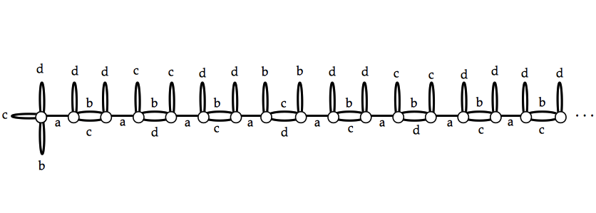
Figure 1.1. Orbital Schreier graph of the right most ray $o=1^{\infty}$ under the action of the first Grigorchuk group.

The first Grigorchuk group $G$ is generated by four automorphisms $a,b,c,d$ of the rooted binary tree (in Subsection 2.4 we recall the definition of these automorphisms, see also Figure 2.1). The group $G$ acts on the boundary of the tree $\partial\mathsf{T}$ by homeomorphisms. The orbital Schreier graph $\mathcal{S}$ of $o$ is a half line as shown in Figure 1.1, where $o=1^{\infty}$ is the right most ray of the tree.

In [Erschler04] random walks with non-trivial Poisson boundary are used to show that for $G_{\omega}$, where $\omega$ is not eventually constant and contains only finite number of ${\bf 2}$ (for example $\omega=({\bf 01})^{\infty}$), its volume growth satisfies

$$v_{G_{\omega},S}(n)\geq\exp\left(c_{\epsilon}n/\log^{1+\epsilon}n\right).$$

The measures with non-trivial Poisson boundary constructed in [Erschler04] come from transient symmetric random walks on $\mathbb{Z}$, where it is well-known and easy to see what is the best tail condition on such measures on $\mathbb{Z}$. The situation remained completely unclear for other Grigorchuk groups with $\omega$ containing all three letters infinitely often. Since for such $\omega$ the group $G_{\omega}$ is torsion, the argument in [Erschler04] relying on an infinite order element cannot be applied. Here we need to introduce a new construction of measures for the first Grigorchuk group.

Consider the groupoid of germs of the action $G\curvearrowright\partial\mathsf{T}$. The isotropy group $\mathcal{G}_{x}$ of the groupoid of germs of $G$ at $x\in\partial\mathsf{T}$ is the quotient of the stabilizer $G_{x}$ of $x$ by the subgroup of elements of $G$ that act trivially in a neighborhood of $x$. For the first Grigorchuk group $G$, at $x$ in the orbit $o\cdot G$, $\mathcal{G}_{x}$ is isomorphic to $\left(\mathbb{Z}/2\mathbb{Z}\right)\times\left(\mathbb{Z}/2\mathbb{Z}\right)$ and its elements can be listed as $\{id,b,c,d\}$. See more details in Section 3. Given a group element $g$, we denote its germ at $x$ by $\Phi_{g}(x)$, which is the germ of $g\tau^{-1}$ in the neighborhood of $x$ where $\tau$ is a finitary automorphism of the tree such that $x\cdot g=x\cdot\tau$. This does not depend on the choice of $\tau$, see precise definition in formula (3.3)). Our goal is to construct a non-degenerate probability measure $\mu$ on $G$ such that along the $\mu$-random walk trajectory $(W_{n})_{n=1}^{\infty}$, the coset of $\Phi_{W_{n}}(o)$ in $\mathcal{G}_{o}/\left\langle b\right\rangle$ stabilizes with probability $1$. Such almost sure stabilization provides non-trivial events in the tail $\sigma$-field of the random walk, which implies the Poisson boundary of $(G,\mu)$ is non-trivial.

Our first construction of a measure with controlled (but not near optimal) tail decay and non-trivial Poisson boundary on $G$ is of the form $\mu=\frac{1}{2}({\bf u}_{S}+\eta)$, where ${\bf u}_{S}$ is the uniform measure on $S=\{a,b,c,d\}$ and $\eta$ is a symmetric measure supported on the subgroup ${\rm H}^{b}$ of $G$. Here ${\rm H}^{b}$ is the subgroup of $G$ that consists of $g\in G$ such that germs $\Phi_{g}(x)$ are in $\left\langle b\right\rangle$ for all $x\in o\cdot G$. For such a measure $\mu$, if the $\eta$-induced random walk on the orbit of $o$ is transient, then the Poisson boundary of $\mu$ is non-trivial, see Remark 3.4. In the situation of $\omega$ containing only ${\bf 0}$ and ${\bf 1}$ infinitely often, the subgroup ${\rm H}^{b}$ contains an infinite order element $ab$, thus in this case one can apply well known results for random walks on $\left\langle ab\right\rangle=\mathbb{Z}$. For the first Grigorchuk group, the subgroup ${\rm H}^{b}$ is locally finite and the orbit of $o$ under ${\rm H}^{b}$ is not the full orbit $o\cdot G$, but rather rays cofinal with $1^{\infty}$ such that at locations $3k+1$, $k\geq 1$, the digits are $1$ (see Lemma 6.2).

Since the subgroup ${\rm H}^{b}$ is locally finite, unlike $\mathbb{Z}$ there is no "simple random walk" on it that one can take convex combinations of convolution powers of the corresponding measure to produce a measure with transient induced random walk on the orbit of $o$. Rather, we build the measures from a sequence of group elements satisfying an injectivity property for their action on the orbit $o\cdot G$. For $g_{1},g_{2},\ldots\in G$, we say the sequence satisfies the cube independence property on $o\cdot G$ if for any $n\geq 1$ and $x\in o\cdot G$, the map from the hypercube to the orbit $\{0,1\}^{n}\to o\cdot G$

$$(\varepsilon_{1},\ldots\varepsilon_{n})\mapsto x\cdot g_{n}^{\varepsilon_{n}}\ldots g_{1}^{\varepsilon_{1}}$$

is injective. We call the set $F_{n}=\left\{g_{n}^{\varepsilon_{n}}\ldots g_{1}^{\varepsilon_{1}}:(\varepsilon_{1},\ldots\varepsilon_{n})\in\{0,1\}^{n}\right\}$ an $n$-quasi-cubic set and the uniform measure ${\bf u}_{F_{n}}$ on $F_{n}$ an $n$-quasi-cubic measure. Given such a sequence $\left(g_{n}\right)$, we take convex combination over all $n$-quasi-cubic measures and their inverses. The cube independence property guarantees that for such measures, the induced random walks on the orbit of $o$ satisfy good isoperimetric inequalities. We prove a sufficient criterion for such induced random walks to be transient in Proposition 5.4.

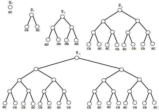
Figure 1.2. Portrtraits of $g_{j},\ j=0,\dots,4$ in the first Grigorchuk group. More generally, words $\zeta^{n}(ax)$, where $x=c$ or $x=d$, represents an element in the stabilizer of level $n$, and the labels (sections) at the vertices of level $n$ are $ax$ or $xa$.

Our choice of elements satisfying the cube independence property on $G$ is closely related to words that are known to have what is called asymptotically maximal inverted orbit growth, see [BE1]. Let $\zeta$ be the substitution on $\{ab,ac,ad\}^{\ast}$ defined as

(1.2) $$\zeta:ab\mapsto abadac,\ ac\mapsto abab,\ ad\mapsto acac.$$

Then $(\zeta^{n}(ac))_{n=1}^{\infty}$ achieves asymptotic maximal inverted orbit growth, see the proof of [BE1, Proposition 4.7]. With considerations of germs in mind, we take the sequence to be $g_{n}=\zeta^{n}(ac)$ if $n\equiv 0,1\mod 3$ and $g_{n}=\zeta^{n}(ad)$ if $n\equiv 2\mod 3$, see Figure 1.2. Then $g_{n}$ has $\left\langle b\right\rangle$-germs for $n\equiv 1,2\mod 3$ and has $\left\langle c\right\rangle$-germs for $n\equiv 0\mod 3$. For our construction it is important that this sequence $\left(g_{n}\right)$ satisfies the cube independence property. As an illustration of Proposition 5.4, in Subsection 5.2 we find an optimal moment condition for measures on $G$ which induce transient random walks on the orbit of $o=1^{\infty}$. Such a measure can be taken to be of the form

$$\eta_{0}=\sum_{n=1}^{\infty}c_{n}\left({\bf u}_{F_{n}}+{\bf u}_{F_{n}^{-1}}\right),$$

where $c_{n}=\frac{C_{\epsilon}n^{1+\epsilon}}{2^{n}}$ , $F_{n}$ is the $n$-quasi-cubic set formed by $g_{1},\ldots,g_{n}$ and ${\bf u}_{F}$ is the uniform measure on $F$.

In Section 6 we explain how to use the subsequence $g_{1},g_{2},g_{4},g_{5},g_{7},g_{8},\ldots$ of only $\left\langle b\right\rangle$-germs and a related sequence that is more adapted to ${\rm H}^{b}$ to produce finite entropy symmetric measures supported on ${\rm H}^{b}$ such that the induced random walks on the orbit of $o$ are transient. In particular it already provides a volume lower bound $\exp\left(cn^{0.57}\right)$ for $G$ better than previously known bounds, see Corollary 6.4.

However taking a measure supported on ${\rm H}^{b}$ is too restrictive, see the remark at the end of Section 6. In Section 7 we carry out the main construction which removes this restriction and produces measures with non-trivial Poisson boundary and near optimal tail decay.

We now give an informal sketch of the construction. Return to the "full" cube independent sequence $(g_{n})_{n=1}^{\infty}$. The measure $\eta_{0}$ built from this sequence has near optimal tail decay among measures that induce transient random walks on the Schreier graph. However in the sequence we have germs of both types: $g_{n}$ has $\left\langle b\right\rangle$-germs for $n\equiv 1,2\mod 3$ and has $\left\langle c\right\rangle$-germs for $n\equiv 0\mod 3$. One can check that $\left\langle\gamma\right\rangle$-coset of $\Phi_{W_{n}}(o)$ does not stabilize for any $\gamma\in\{b,c,d\}$, where $W_{n}$ is the random walk driven by $\frac{1}{2}({\bf u}_{S}+\eta_{0})$. With the goal to achieve almost sure stabilization of $\left\langle b\right\rangle$-coset of $\Phi_{W_{n}}(o)$ along the random walk trajectory, we want to perform modifications to the elements used in the construction of $\eta_{0}$ that prevent such stabilization, namely these $g_{n}$ with $\left\langle c\right\rangle$-germs.

It turns out for such considerations, transience of the induced random walks on the Schreier graph is not sufficient. To observe almost sure stabilization of $\left\langle b\right\rangle$-coset of $\Phi_{W_{n}}(o)$ for a $\mu$-random walk $W_{n}$, we need to show a weighted sum of the Green function $\mathbf{G}_{P_{\mu}}$ over the Schreier graph is finite, see the criterion in Proposition 3.3:

$$\sum_{x\in o\cdot G}\mathbf{G}_{P_{\mu}}(o,x)\mu\left(\left\{g\in G:\ (g,x)\mbox{ is not a }\left\langle b\right\rangle\mbox{-germ}\right\}\right)<\infty.$$

Thus the behavior of the Green function of the induced random walk is essential. Informally we call a ray $x\in\partial\mathsf{T}$ that carries a non-$\left\langle b\right\rangle$ germ a bad location. Assume that the Green function $\mathbf{G}_{P_{\mu}}(o,x)$ decays with distance $d_{\mathcal{S}}(o,x)$, then to control the effect of $\left\langle c\right\rangle$-germ elements, it is to our advantage to push the bad locations to be further away from the ray $o$. Note that when we perform modifications to the measure, all terms in the summation are affected: both the Green function of $P_{\mu}$ and the $\mu$-weights on the bad locations.

Recall that for $n$ divisible by $3$, $g_{n}=\zeta^{n}(ac)$, it is in the $n$-level stabilizer and the section at any vertex $v$ in level $n$ is in $\{ac,ca\}$. Therefore $g_{n}$ has $2^{n}$ bad locations on the Schreier graph and the distance of these locations to $o$ is bounded by $C2^{n}$. To move these locations further from $o$, without causing disturbances globally, we rely on certain branching properties of the group. Let $k_{n}$ be an integer divisible by $3$, we introduce a conjugation of the generator $c$ that swaps on level $k_{n}+2$ the section at $1^{k_{n}+2}$ with the section at its sibling. Explicitly, take the element $h_{k_{n}}$ which is in the rigid stabilizer of $1^{k_{n}}$ and acts as $baba$ in the subtree rooted at $1^{k_{n}}$. Denote by $\mathfrak{c}_{k_{n}}$ the conjugate $\mathfrak{c}_{k_{n}}=h_{k_{n}}^{-1}ch_{k_{n}}$. The portrait of $\mathfrak{c}_{k_{n}}$ is illustrated in Figure 1.3. For $n$ and $k_{n}$ both divisible by $3$, take $\tilde{g}_{n}=\zeta^{n}\left(a\mathfrak{c}_{k_{n}}\right)$. Then $\tilde{g}_{n}$ still has $2^{n}$ locations on the Schreier graph such that $(\tilde{g}_{n},x)$ is a $c$-germ, but now the distance of these locations to $o$ is comparable to $2^{n+k_{n}}$.

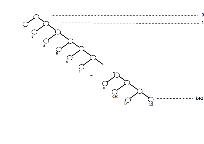
Figure 1.3. A portrtrait of $\mathfrak{c}_{k}$, for $k\equiv 0\mod 3$. There are $k+3$ levels of the tree shown on the picture. The portrait is the same as the portrait of $c$ up to level $k$, while at level $k+2$ left and right branches are permuted.

Take a parameter sequence $(k_{n})$, in the cube independent sequence $(g_{n})$, keep these $g_{n}$ such that $n\equiv 1,2\mod 3$ and replace these $g_{n}$ with $n\equiv 0\mod 3$ by the modified element $\tilde{g}_{n}$. This modified sequence satisfies the cube independence property, we can form the $n$-quasi-cubic sets and define a measure $\eta$ of the same form as $\eta_{0}$ using this sequence. It is possible that with some choice like $c_{n}=2^{-n\beta}$, $\beta$ close to $1$ and $k_{n}=A\log n$, one can observe almost sure stabilization for the resulting measure $\frac{1}{2}({\bf u}_{S}+\eta)$. However for such a measure $\mu$ we didn’t manage to obtain good enough estimates on the induced Green function to verify the summability condition. Here the issue is that because of the modifications, the induced transition kernel on the Schreier graph becomes more singular (compared to the one induced by $\eta_{0}$ ).

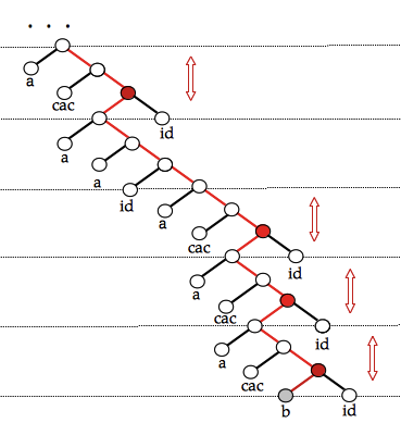
Figure 1.4. A conjugated element $\mathfrak{c}^{v}$, in usual notation on the first Grigorchuk group. The levels of the form $3j-1$ are traced with dotted lines. There are two possiblities for the portraits between $3j-1$ and $3j+2$. Here the picture is shown for indexing vertex $v=11(11\ast)\dots(11\ast)(110)(111)(110)(110)110$.

To overcome this difficulty, we introduce an extra layer of randomness to produce less singular induced transition kernels. We take a collection of conjugates $\mathfrak{c}^{v}$ of $c$, indexed by vertices $v$ of the form $11\underbrace{11\ast 11\ast\ldots 11\ast}_{k_{n}\ {\rm digits}}110$, where at $\ast$ the digit can be $0$ or $1$, see Figure 1.4. Given such a conjugate $\mathfrak{c}^{v}$, as before apply the substitution $\zeta$ to obtain $\tilde{g}_{n}^{v}=\zeta^{n}\left(a\mathfrak{c}^{v}\right)$. We call an $n$-quasi-cubic set formed by $\left(\tilde{g}_{j}^{v}\right)$ with each $v$ a random vertex chosen uniformly from the corresponding indexing set a uniformised quasi-cubic set. The final measure we take to prove Theorem A is of a similar form to $\eta$ discussed in the previous paragraph, but involves what we call uniformised quasi-cubic measures. For more detailed description of these measures see Example 7.10. We remark that the parameters $\left(k_{n}\right)$ need to be chosen carefully: the word length of element $\tilde{g}_{n}$ is approximately $2^{k_{n}}(2/\eta_{0})^{n}$, therefore if $k_{n}$ is too large, the tail decay wouldn’t be near $n^{-\alpha_{0}}$; on the other hand if $k_{n}$ is not sufficiently large then the effect it introduces is not strong enough to achieve the goal of stabilization. In the end we will take $k_{n}\approx A\log n$ with constant $A$ large enough.

After the extra randomization, the resulting measure on $G$ induces a transition kernel on the Schreier graph to which known heat kernel estimates can be applied. More precisely, we apply techniques from Barlow-Grigor’yan-Kumagai [BGK] based on what is called the Meyer’s construction and the Davies method for off-diagonal heat kernel estimates of jumping processes. In this way we obtain good enough decay estimate for the induced Green function in terms of the Schreier graph distance on the orbit of $o$. Together with explicit estimates of the $\mu$-weights at bad locations we show the weighted sum of Green function over the Schreier graph is finite with appropriate choice of parameters. The construction provides finite entropy measures on $G$ with near optimal tail decay and non-trivial Poisson boundary.

1.2. Organization of the paper

Section 2 reviews background on Poisson boundary and its connection to growth, groups acting on rooted trees and some basic properties of Grigorchuk groups. In Section 3 we formulate the criterion for stabilization of cosets of germ configurations. Section 4 provides quick examples of measures (without explicit tail control) with non-trivial Poisson boundary on the first Grigorchuk group. In Section 5 we define the cube independence property and show how to build explicit measures with transient induced random walks from sequences satisfying this property. Section 6 discusses measures with restricted germs on the first Grigorchuk group that induce transient random walks on the orbit of $1^{\infty}$, in particular volume lower bounds such measures provide and their limitations. Section 7 contains the main result of the paper: we construct finite entropy measures on $G_{\omega}$ with near optimal tail decay and non-trivial Poisson boundary, where $\omega$ satisfies what we call Assumption $({\rm Fr}(D))$. In Section 8 we derive volume lower estimates for $G_{\omega}$ from measures constructed in Section 7. We close the paper with a few remarks and questions.

Conventions that are used throughout the paper:

• We consider right group actions $\Gamma\curvearrowright X$ and write the action of group element $g$ on $x\in X$ as $x\cdot g$.

• Given a probability measure $\mu$ on $\Gamma$, we say $\mu$ is non-degenerate if its support generates $G$ as a semigroup. Let $X_{1},X_{2},\ldots$ be i.i.d. random variables with distribution $\mu$ on $\Gamma$ and $W_{n}=X_{1}\ldots X_{n}$. We refer to $(W_{n})_{n=1}^{\infty}$ as a $\mu$-random walk.

• On a regular rooted tree $\mathsf{T}$, given a vertex $u\in\mathsf{T}$ and $v\in\mathsf{T}\cup\partial\mathsf{T}$, $uv$ denotes the concatenation of the strings, that is the ray with prefix $u$ followed by $v$. Given $u,v\in\mathsf{T}\cup\partial\mathsf{T}$, $u\wedge v$ denotes the longest common prefix of $u$ and $v$.

• Given a finite set $F$, ${\bf u}_{F}$ denotes the uniform distribution on $F$.

• Let $v_{1},v_{2}$ two non-decreasing functions on $\mathbb{N}$ or $\mathbb{R}$, $v_{1}\lesssim v_{2}$ if there is a constant $C>0$ such that $v_{1}(x)\leq v_{2}(Cx)$ for all $x$ in the domain. Let $\simeq$ be the equivalence relation that $v_{1}\simeq v_{2}$ if $v_{1}\lesssim v_{2}$ and $v_{2}\lesssim v_{1}$. Note that for finitely generated infinite groups, the $\simeq$ equivalence class of the growth function does not depend on the choice of generating set.

Acknowledgment

We are grateful to the anonymous referee whose comments and suggestions improved the exposition of the paper. We thank Jérémie Brieussel for helpful comments on the preliminary version of the paper.

2. Preliminaries

2.1. Boundary behavior of random walks and connection to growth

We recall the notion of the invariant $\sigma$-field and the tail $\sigma$-field of a random walk. Let $\mu$ be a probability measure on a countable group $\Gamma$. For $x\in\Gamma$, let $\mathbb{P}_{x}$ be the law of the random walk trajectory $\left(W_{0},W_{1},\ldots\right)$ starting at $W_{0}=x$. Endow the space of infinite trajectories $G^{\mathbb{N}}$ with the usual Borel $\sigma$-field $\mathcal{A}$. The shift $\mathfrak{s}:\Gamma^{\mathbb{N}}\to\Gamma^{\mathbb{N}}$ acts by $\mathfrak{s}(g_{1},g_{2},\ldots)=(g_{2},g_{3},\ldots)$. The invariant $\sigma$-field $\mathcal{I}$ is defined as $\mathcal{I}=\{A\in\mathcal{A:\ \mathfrak{s}}^{-1}(A)=A\}$, it is also referred to as the stationary $\sigma$-field. There is a correspondence between $\mathcal{I}$ and the space of bounded $\mu$-harmonic functions on $\Gamma$. In particular, the invariant $\sigma$-field $\mathcal{I}$ is trivial (i.e. any event $A\in\mathcal{I}$ satisfies $\mathbb{P}_{x}(A)=0$ or $1$) if and only if all bounded $\mu$-harmonic functions are constant, see [KV83].

The intersection $\mathcal{A}_{\infty}=\cap_{n=0}^{\infty}\mathfrak{s}^{-n}\mathcal{A}$ is called the tail $\sigma$-field or exit $\sigma$-field of the random walk. When $\mu$ is aperiodic, the $\mathbb{P}_{x}$-completion of $\mathcal{A}_{\infty}$ and the $\mathbb{P}_{x}$-completion of $\mathcal{I}$ coincide. Therefore for $\mu$ aperiodic, all bounded $\mu$-harmonic functions are constant if and only if the tail $\sigma$-field $\mathcal{A}_{\infty}$ is $\mathbb{P}_{x}$-trivial for some (hence all ) $x\in\Gamma$.

The (Shannon) entropy of a probability measure $\mu$ on $\Gamma$ is

$$H(\mu)=-\sum_{g\in\Gamma}\mu(g)\log\mu(g).$$

In the case that the measure $\mu$ has finite entropy $H(\mu)<\infty$, the (Avez) asymptotic entropy of $\mu$ is defined as

$$\mathbf{h}_{\mu}=\lim_{n\to\infty}\frac{H\left(\mu^{(n)}\right)}{n}.$$

The entropy criterion of Kaimanovich-Vershik [KV83] and Derriennic [derriennic], states that for $\mu$ of finite entropy, all bounded $\mu$-harmonic functions are constant if and only if the Avez asymptotic entropy $\mathbf{h}_{\mu}=0$.

Given a probability measure of finite entropy and non-trivial Poisson boundary on a finitely generated group $\Gamma$, by the entropy criterion and the Shannon theorem, one can derive lower estimate for the volume growth of $\Gamma$ from the tail decay of the measure. The following lemma extends [Erschler04, Lemma 6.1].

Lemma 2.1.

Let $\Gamma$ be a finitely generated group and $\left|\cdot\right|=l_{S}$ a word distance on $\Gamma$. Suppose $\Gamma$ admits a probability measure $\mu$ of finite entropy such that the Poisson boundary $(\Gamma,\mu)$ is nontrivial. Let

$$\varrho_{n}=\inf\left\{r>0:\ \mu\left(\left\{g:|g|\geq r\right\}\right)<1/n\right\}\mbox{ and }\ \phi(r)=\sum_{g:|g|\leq r}|g|\mu(g).$$

Then there exists a constant $c=c(\Gamma,\mu)>0$ such that

$$v_{\Gamma,S}(R_{n})\geq\exp\left(cn\right)\ \mbox{where }R_{n}=n\phi(\varrho_{n}).$$

Proof.

If the measure $\mu$ has finite first moment, in other words the function $\phi(r)$ is bounded, then $\Gamma$ has exponential growth. In this case the claim is true. In what follows we assume that $\phi(r)\to\infty$ as $r\to\infty$.

Let $\mu_{\varrho}$ be the truncation of measure $\mu$ at radius $\varrho$, that is $\mu_{\varrho}(g)=\mu(g)\mathbf{1}_{\{|g|\leq\varrho\}}$. Because of the triangle inequality $|gh|\leq|g|+|h|$, we have

$$\sum_{g}|g|\mu_{\varrho}^{(n)}(g)\leq n\sum_{g}|g|\mu_{\varrho}(g)=n\phi(\varrho).$$

It follows from Markov inequality that

$$\mu_{\varrho}^{(n)}(\{g:\ |g|\geq R\})\leq\frac{n\phi(\varrho)}{R}.$$

For all $n\geq 2$ , the total mass of the convolution power $\mu_{\varrho_{n}}^{(n)}$ satisfies

$$\sum_{g}\mu_{\varrho_{n}}^{(n)}(g)=\left(1-\mu(\{g:|g|>\varrho_{n}\})\right)^{n}\geq(1-1/n)^{n}\geq\frac{1}{4}.$$

Take $R_{n}=8n\phi(\varrho_{n})$, then

$$\mu^{(n)}(B(e,R_{n}))\geq\mu_{\varrho_{n}}^{(n)}(B(e,R_{n}))\geq\frac{1}{4}-\frac{n\phi(\varrho_{n})}{R_{n}}=\frac{1}{8}.$$

Denote by $\mathbf{h}$ the asymptotic entropy of $\mu$. By the entropy criterion, non-triviality of Poisson boundary of $(G,\mu)$ is equivalent to $\mathbf{h}>0$. By Shannon’s theorem, for any $\epsilon>0$, there exists a constant $N_{\epsilon}$ such that for any $n>N_{\epsilon}$, there is a finite set $V_{n}\subset G$ such that $\mu^{(n)}(V_{n})\geq 1-\epsilon$ and

$$e^{-n(\mathbf{h}+\epsilon)}\leq\mu^{(n)}(x)\leq e^{-n(\mathbf{h}-\epsilon)}\mbox{ for }x\in V_{n}.$$

Consider the intersection $V_{n}^{\prime}=\{g:\ |g|\leq R_{n}\}\cap V_{n}$, we have

$$\frac{1}{8}-\epsilon\leq\mu^{(n)}(V_{n}^{\prime})\leq|V_{n}^{\prime}|\max_{g\in V_{n}^{\prime}}\mu^{(n)}(g)\leq|V_{n}^{\prime}|e^{-n(\mathbf{h}-\epsilon)}.$$

Choose $\epsilon>0$ to be a constant less than $\frac{1}{2}\min\{1/8,\mathbf{h}\}$. We obtain that for all $n$ sufficiently large,

$$v_{\Gamma,S}(R_{n})\geq|V_{n}^{\prime}|\geq\frac{1}{16}e^{\frac{1}{2}n\mathbf{h}}.$$

∎

We record the following two corollaries of Lemma 2.1.

Corollary 2.2.

Suppose that $\Gamma$ admits a probability measure $\mu$ of finite entropy with nontrivial Poisson boundary. Suppose $\mu$ satisfies

$$\mu\left(\{g:|g|\geq r\}\right)\leq\frac{C}{r^{\alpha}\ell(r)},$$

where $\alpha\in(0,1)$ and $\ell$ is a slowly varying function such that $\ell(x)\sim\ell(x^{b})$ as $x\to\infty$ for some $b>0$. Then there exists a constant $c=c(\Gamma,\mu)>0$ such that

$$v_{\Gamma,S}(n)\geq\exp(cn^{\alpha}\ell(n)).$$

Proof.

Let $f$ be the asymptotic inverse of $r^{\alpha}\ell(r)$, then $f(r)\sim(r\ell^{\#}(r))^{1/\alpha}$, where $\ell^{\#}$ is the de Bruijn conjugate of $\ell,$ see [RV, Proposition 1.5.15.]. Let

$$\tilde{\phi}(r)=\int_{1}^{r}\frac{dx}{x^{\alpha}\ell(x)}.$$

Then $\tilde{\phi}(r)\sim\frac{1}{1-\alpha}r^{1-\alpha}/\ell(r)$, see [RV, Proposition 1.5.8.]. It follows that

$$R_{n}=4n\phi(\varrho_{n})\leq C_{1}n\tilde{\phi}(f(n))\leq C_{2}n^{1/\alpha}\ell^{\#}(n)^{-1+1/\alpha}/\ell(n^{1/\alpha}\ell^{\#}(n)^{1/\alpha}).$$

Under the assumption that $\ell(x)\sim\ell(x^{b})$ for some $b>0$, we have $\ell^{\#}(x)\sim 1/\ell(x)$ and the bound simplifies to

$$R_{n}\leq C(n/\ell(n))^{1/\alpha}.$$

By Lemma 2.1, there exists constants $C,c>0$ which depend on $\mu$ such that

$$v_{\Gamma,S}\left(C(n/\ell(n))^{1/\alpha}\right)\geq\exp(cn).$$

Since the asymptotic inverse of $(x/\ell(x))^{1/\alpha}$ is $x^{\alpha}\ell(x)$ in this case, we conclude that there exists a constant $c=c(\Gamma,\mu)>0$ such that

$$v_{\Gamma,S}(n)\geq\exp(cn^{\alpha}\ell(n)).$$

∎

Corollary 2.3.

Let $\Gamma$ be a finitely generated group such that $v_{\Gamma}(r)\lesssim\exp(r^{\alpha})$, where $\alpha\in(0,1)$. Then any probability measure $\mu$ on $\Gamma$ with finite $\alpha$-moment

$$\sum_{g\in\Gamma}|g|^{\alpha}\mu(g)<\infty$$

has finite entropy and trivial Poisson boundary.

Proof.

We first show that $\mu$ has finite entropy. Write $M=\sum_{g\in\Gamma}|g|^{\alpha}\mu(g)$. Denote by $\mu_{k}$ the restriction of $\mu$ to $B\left(e,2^{k}\right)\setminus B(e,2^{k-1})$, normalized to be a probability measure, that is $\mu_{k}(g)=\frac{1}{\lambda_{k}}\mu(g)\mathbf{1}_{B\left(e,2^{k}\right)\setminus B(e,2^{k-1})}$, where $\lambda_{k}=\mu\left(B\left(e,2^{k}\right)\setminus B(e,2^{k-1}\right)$. It follows that $\mu=\sum_{k=0}^{\infty}\lambda_{k}\mu_{k}$. Recall the fact that the entropy of any probability measure supported by a finite set is maximal for the uniform measure. Let $X_{1}$ be a random variable with distribution $\mu$ and $Z=\sum_{k=1}^{\infty}k\mathbf{1}_{B\left(e,2^{k}\right)\setminus B(e,2^{k-1})}(X_{1})$. Then

$$H(\mu) \leq\sum_{k=0}^{\infty}\lambda_{k}H(\mu_{k})+\sum_{k=0}^{\infty}-\lambda_{k}\log\lambda_{k}$$

$$\leq\sum_{k=0}^{\infty}\lambda_{k}\log\left|B(e,2^{k})\right|+\sum_{k=0}^{\infty}-\lambda_{k}\log\lambda_{k}.$$

Now we plug in the assumption on the volume function of $\Gamma$ that $\left|B(e,2^{k})\right|\leq\exp(Cr^{\alpha})$ for some constant $C$, then

$$\sum_{k=0}^{\infty}\lambda_{k}\log\left|B(e,2^{k})\right|\leq C\sum_{k=0}^{\infty}\lambda_{k}2^{k\alpha}\leq 2^{\alpha}C\sum_{g\in\Gamma}|g|^{\alpha}\mu(g)=2^{\alpha}CM.$$

By the Markov inequality we have $\lambda_{k}\leq\frac{M}{2^{(k-1)\alpha}}$. Then for the second term, by the inequality $-a\log a\leq 2e^{-1}\sqrt{a}$, we have

$$\sum_{k=0}^{\infty}-\lambda_{k}\log\lambda_{k}\leq\sum_{k=0}^{\infty}2e^{-1}\sqrt{\lambda_{k}}\leq 2e^{-1}\sqrt{M}\sum_{k=0}^{\infty}2^{-\frac{(k-1)\alpha}{2}}<\infty.$$

We conclude that $\mu$ has finite entropy.

Suppose on the contrary $\mu$ has non-trivial Poisson boundary. Since $\mu$ has finite $\alpha$-moment, we have

$$\varrho_{n} =\inf\{r:\ \mu(\{g:|g|\geq r\})\leq 1/n\}\leq n^{1/\alpha},$$

$$\phi(r) =\sum_{g:|g|\leq r}|g|\mu(g)=o(r^{1-\alpha})\mbox{ as }r\to\infty.$$

Therefore by Corollary 2.2, we have that $v_{\Gamma}(R_{n})\gtrsim e^{n}$ where $R_{n}/n^{1/\alpha}\to 0$ as $n\to\infty$. This contradicts with the assumption that $v_{\Gamma}(r)\lesssim\exp(r^{\alpha})$.

∎

2.2. Permutational wreath products

Let $\Gamma$ be a group acting on a set $X$ from the right. Let $A$ be a group, the permutational wreath product $W=A\wr_{X}\Gamma$ is defined as the semi-direct product $\sum_{X}A\rtimes\Gamma$, where $\Gamma$ acts on $\sum_{X}A$ by permuting coordinates. The support ${\rm supp}f$ of $f:X\to A$ consists of points of $x\in X$ such that $f(x)\neq id_{A}$. Elements of $\sum_{X}A$ are viewed as finitely supported functions $X\to A$. The action of $\Gamma$ on $\sum_{X}A$ is

$$\tau_{g}f(x)=f(x\cdot g).$$

It follows that ${\rm supp}(\tau_{g}f)=({\rm supp}f)\cdot g^{-1}$. Elements in $W=A\wr_{X}\Gamma$ are recorded as pairs $(f,g)$ where $f\in\sum_{X}A$ and $g\in\Gamma$. Multiplication in $W$ is given by

$$(f_{1},g_{1})(f_{2},g_{2})=(f_{1}\tau_{g_{1}}f_{2},g_{1}g_{2}).$$

When $\Gamma$ and $A$ are finitely generated, $W=A\wr_{X}\Gamma$ is finitely generated as well. For more information about Cayley graphs of permutational wreath products, see [BE1, Section 2].

2.3. Groups acting on rooted trees

We review some basics for groups acting on rooted trees. For more background and details, we refer to [BGShandbook, Part 1] or [NekraBook, Chapter 1]. Let $\mathbf{d}=(d_{j})_{j\in\mathbb{N}}$ be a sequence of integers, $d_{j}\geq 2$ for all $j\in\mathbb{N}$.

The spherically symmetric rooted tree $\mathsf{T}_{\mathbf{d}}$ is the tree with vertices $v=v_{1}\ldots v_{n}$ with each $v_{j}\in\{0,1,\ldots,d_{j}-1\}$. The root is denoted by the empty sequence $\emptyset$. Edge set of the tree is $\left\{\left(v_{1}\ldots v_{n},v_{1}\ldots v_{n}v_{n+1}\right)\right\}$. The index $n$ is called the depth or level of $v$, denoted $\left|v\right|=n$. Denote by $\mathsf{T}_{\mathbf{d}}^{n}$ the finite subtree of vertices up to depth $n$ and $\mathsf{L}_{n}$ the vertices of level $n$. The boundary $\partial\mathsf{T}_{\mathbf{d}}$ of the tree $\mathsf{T}_{\mathbf{d}}$ is the set of infinite rays $x=v_{1}v_{2}\ldots$ with $v_{j}\in\{0,1,\ldots,d_{j}-1\}$ for each $j\in\mathbb{N}$.

The group of automorphisms ${\rm{Aut}}(\mathsf{T}_{\mathbf{d}})$ of the rooted tree is the group of tree automorphisms that fix the root $\emptyset$. The group ${\rm{Aut}}(\mathsf{T}_{\mathbf{d}})$ admits the following canonical isomorphism

$$\psi:{\rm Aut}(\mathsf{T}_{\mathbf{d}})\to{\rm Aut}(\mathsf{T}_{\mathbf{\mathfrak{s}d}})\wr_{\{0,1,\ldots,d_{1}-1\}}\mathfrak{S}_{d_{1}},$$

where $\mathfrak{S}_{d}$ is the permutation group on the set $\{0,1,\ldots,d-1\}$, and $\mathfrak{s}$ is the shift on the sequences, $\mathfrak{s}(d_{1},d_{2},\ldots)=(d_{2},d_{3},\ldots)$. We refer to the isomorphism $\psi$ as the wreath recursion. As the isomorphism is canonical, we omit $\psi$ and identify an automorphism and its image under $\psi$: for $g\in{\rm Aut}(\mathsf{T}_{\mathbf{d}})$, write

$$g=\left(g_{0},\ldots,g_{d_{1}-1}\right)\tau_{1}(g)$$

where the sections $g_{j}\in{\rm Aut}(\mathsf{T}_{\mathfrak{s}\mathbf{d}})$ and $\tau_{1}(g)\in S_{d_{1}}$. The section $g_{j}$ represents the action of $g$ on the subtree $\mathsf{T}_{j}$ rooted at the vertex $j$. The permutation $\tau_{1}(g)$ describes how the subtrees rooted at $j$, $j\in\{0,1,\ldots,d_{1}-1\}$ are permuted. We refer to $\tau_{1}(g)$ as the root permutation of $g$.

Apply the wreath recursion $n$ times, we have

$$\psi^{n}:{\rm Aut}(\mathsf{T}_{d}) \to{\rm Aut}(\mathsf{T}_{\mathfrak{s}^{n}{\bf d}})\wr_{\mathsf{L}_{n}}{\rm Aut}(\mathsf{T}_{\mathbf{d}}^{n}),$$

$$g \mapsto(g_{v})_{v\in\mathsf{L}_{n}}\tau_{n}(g),$$

where finitary permutation $\tau_{n}(g)$ is the projection of $g$ to the automorphism group of the finite tree $\mathsf{T}_{\mathbf{d}}^{n}$, and $g_{v}$ is called the section of $g$ at vertex $v$. Since the isomorphism $\psi^{n}$ is canonical, we write $g=(g_{v})_{v\in\mathsf{L}_{n}}\tau_{n}(g)$.

Let $G$ be a subgroup of ${\rm{Aut}}(\mathsf{T}_{\mathbf{d}})$. Given a vertex $u\in\mathsf{T}_{\mathbf{d}}$, the vertex stabilizer ${\rm St}_{G}(u)$ consists of these elements in $G$ that fix $u$, that is ${\rm St}_{G}(u)=\{g\in G:\ u\cdot g=u\}$. The $n$-th level stabilizer ${\rm St}_{G}(\mathsf{L}_{n})$ consists of the automorphisms in $G$ that fix all the vertices on level $n$:

$${\rm St}_{G}(\mathsf{L}_{n}):=\cap_{v\in\mathsf{L}_{n}}{\rm St}_{G}(v).$$

The rigid vertex stabilizer of $u$ in $G$, denoted by ${\rm Rist}_{G}(u)$, consists of the automorphisms in $G$ that fix all vertices not having $u$ as a prefix. An element $g\in{\rm Rist}_{G}(u)$ only acts on the subtree rooted at $u$: if $|u|=n$, then under the wreath recursion $\psi^{n}$, the finitary permutation $\tau_{n}(g)$ is equal to identity, and the section $g_{v}$ is equal to identity for any $v\neq u$. Since automorphisms in different rigid vertex stabilizers on the same level act on disjoint subtrees, they commute with other other. The rigid $n$-th level stabilizer is defined as

$${\rm Rist}_{G}(\mathsf{L}_{n}):=\prod_{u\in\mathsf{L}_{n}}{\rm Rist}_{G}(u).$$

We now recall the definitions of branch groups. Let $\mathsf{T}$ be a rooted tree of constant valency $d$ and $G$ be a subgroup of ${\rm{Aut}}(\mathsf{T})$ acting level transitively.

1. If all rigid $n$-th level stabilizers ${\rm Rist}_{G}(\mathsf{L}_{n})$, $n\in\mathbb{N}$, have finite index in $G$, then we say $G$ is a branch group.

2. We say $G$ is a regular branch group if it acts on a regular tree $\mathsf{T}$ of constant valency $d$, and there exists a finite index subgroup $K<G$ such that $K^{d}$ is contained in $\psi(K)$ as a finite index subgroup, that is $(\underbrace{K,\ldots,K}_{d\ {\rm copies}})$ is a finite index subgroup of $\psi(K)$. In this case we say $G$ is branching over $K$.

The group of automorphisms of the subtree rooted at $u$ is embedded in ${\rm Aut}(\mathsf{T}_{d})$ as rigid vertex stabilizer of $u$ by

(2.1) $$\iota(\cdot:u):{\rm Aut}(\mathsf{T}_{\mathfrak{s}^{n}{\bf d}}^{u}) \to{\rm Aut}(\mathsf{T}_{\mathfrak{s}^{n}{\bf d}})\wr_{\mathsf{L}_{n}}{\rm Aut}(\mathsf{T}_{\mathbf{d}}^{n})$$

$$h \mapsto(g_{v}),\ \mbox{where }g_{u}=h\mbox{ and }g_{v}=e\mbox{ for any }v\neq u.$$

It follows from the definition that if $G$ is branching over $K$, then for any vertex $u\in\mathsf{T}$, ${\rm Rist}_{G}(u)$ contains $K$ as a subgroup. In particular, we have that $\iota(h,u)\in K$ for any $h\in K$, $u\in\mathsf{T}$.

2.4. Grigorchuk groups

The groups $\left\{G_{\omega}\right\}$ were introduced by Grigorchuk in [Grigorchuk84] as first examples of groups of intermediate growth. We recall below the definition of these groups. See also exposition in the books [delaHarpeBook, Chapter VIII] and [Mann].

Let $\{{\bf 0},{\bf 1},{\bf 2}\}$ be the three non-trivial homomorphisms from the $4$-group $(\mathbb{Z}/2\mathbb{Z})\times(\mathbb{Z}/2\mathbb{Z})=\{id,b,c,d\}$ to the $2$-group $\mathbb{Z}/2\mathbb{Z}=\{id,a\}$. They are ordered in such a way that ${\bf 0},{\bf 1},{\bf 2}$ vanish on $d,c,b$ respectively. For example, ${\bf 0}$ maps $id,d$ to $id$ and $b,c$ to $a$. Let $\Omega=\left\{{\bf 0},{\bf 1},{\bf 2}\right\}^{\mathbb{\infty}}$ be the space of infinite sequences over letters $\left\{{\bf 0},{\bf 1},{\bf 2}\right\}$. The space $\Omega$ is endowed with the shift map $\mathfrak{s}:\Omega\to\Omega$, $\mathfrak{s}(\omega_{0}\omega_{1}\ldots)=\omega_{1}\omega_{2}\ldots$.

Given an $\omega\in\Omega$, the Grigorchuk group $G_{\omega}$ acting on the rooted binary tree is generated by $\left\{a,b_{\omega},c_{\omega},d_{\omega}\right\}$, where $a=(id,id)\varepsilon$, $\varepsilon$ transposes $0$ and $1$, and the automorphisms $b_{\omega},c_{\omega},d_{\omega}$ are defined recursively according to $\omega$ as follows. The wreath recursion sends

$$\psi_{n}:G_{\mathfrak{s}^{n}\omega}\to G_{\mathfrak{s}^{n+1}\omega}\wr_{\{0,1\}}\mathfrak{S}_{2}$$

by

$$\psi_{n}\left(b_{\mathfrak{s}^{n}\omega}\right) =\left(\omega_{n}(b),b_{\mathfrak{s}^{n+1}\omega}\right),$$

$$\psi_{n}\left(c_{\mathfrak{s}^{n}\omega}\right) =\left(\omega_{n}(c),c_{\mathfrak{s}^{n+1}\omega}\right),$$

$$\psi_{n}\left(d_{\mathfrak{s}^{n}\omega}\right) =\left(\omega_{n}(d),d_{\mathfrak{s}^{n+1}\omega}\right).$$

The string $\omega$ determines the portrait of the automorphisms $b_{\omega},c_{\omega},d_{\omega}$ by the recursive definition above. The first Grigorchuk group corresponds to the periodic sequence $\omega=({\bf 012})^{\infty}$ and is often denoted as $G_{012}$. See Figure 2.1 for the portraits of these tree automorphisms. The construction of $G_{012}$ is given by Grigorchuk in [Grigorchuk80], where he shows that $G_{012}$ is a torsion group. Merzlyakov has shown later in [Merzlyakov] that the construction of $G_{012}$ is closely related to an earlier construction of Aleshin [Aleshin]. Indeed it can be shown that $G_{012}$ and Aleshin’s group in [Aleshin] are commensurable.

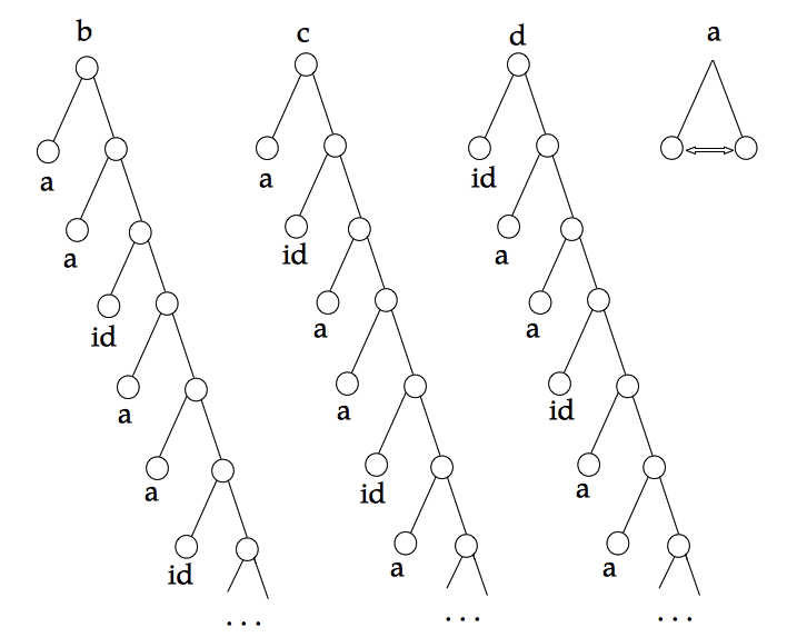
Figure 2.1. Portraits of generators of the first Grigorchuk group.

Main interest in Grigorchuk’s construction results from his paper [Grigorchuk84] where it is shown that $G_{012}$, and more generally $G_{\omega}$ with $\omega$ not eventually constant, is of intermediate growth. If $\omega$ is eventually constant, then $G_{\omega}$ has polynomial growth. When $\omega$ contains infinitely many of each of the three symbols $\{{\bf 0},{\bf 1},{\bf 2}\}$, $G_{\omega}$ is an infinite torsion group.

The following substitutions are used to obtain words with asymptotically maximal inverted orbit growth in [BE2, Section 3.2]. Define self-substitutions $\zeta_{i}$, $i\in\{{\bf 0},{\bf 1},{\bf 2}\}$, of $\{ab,ac,ad\}$ by

(2.2) $$\zeta_{{\bf 0}}:ab\mapsto abab, \ ac\mapsto acac,\ ad\mapsto abadac,$$

$$\zeta_{{\bf 1}}:ab\mapsto abab,\ ac\mapsto adacab,\ ad\mapsto adad,$$

$$\zeta_{{\bf 2}}:ab\mapsto acabad,\ ac\mapsto acac,\ ad\mapsto adad.$$

It is understood that $\zeta_{\omega_{n}}$ sends $\left\{ab_{\mathfrak{s}^{n+1}\omega},ac_{\mathfrak{s}^{n+1}\omega},ad_{\mathfrak{s}^{n+1}\omega}\right\}^{\ast}$ to $\left\{ab_{\mathfrak{s}^{n}\omega},ac_{\mathfrak{s}^{n}\omega},ad_{\mathfrak{s}^{n}\omega}\right\}^{\ast}$ by the rules specified above, for example if $\omega_{n}={\bf 0}$, then $\zeta_{\omega_{n}}\left(ab_{\mathfrak{s}^{n+1}\omega}\right)=ab_{\mathfrak{s}^{n}\omega}ab_{\mathfrak{s}^{n}\omega}$. One step wreath recursion gives that for $w\in\left\{ab,ac,ad\right\}^{\ast}$,

(2.3) $$\psi_{n}(\zeta_{\omega_{n}}\left(w\right))=\begin{cases}(awa,w)&\mbox{if }\zeta_{\omega_{n}}(w)\mbox{ contains an even number of }a,\\ (wa,aw)\varepsilon&\mbox{if }\zeta_{\omega_{n}}(w)\mbox{ contains an odd number of }a.\end{cases}$$

This formula is used in [BE2, Section 3.2] (where there is a misprint), see also lecture notes of Bartholdi [bartholdinote, Section F]. It follows from (2.3) that if $g\in G_{\mathfrak{s}^{n+1}\omega}$ can be represented by a word in $\{ab_{\mathfrak{s}^{n+1}\omega},ac_{\mathfrak{s}^{n+1}\omega},ad_{\mathfrak{s}^{n+1}\omega}\}$, then the substitution $\zeta_{\omega_{n}}$ can be applied to $g$ and the resulting image in $G_{\mathfrak{s}^{n}\omega}$ does not depend on the choice of the representing word. The composition $\zeta_{\omega_{0}}\circ\ldots\circ\zeta_{\omega_{n}}$ maps such $g\in G_{\mathfrak{s}^{n+1}\omega}$ into $G_{\omega}$.

Usually, the recursion on the first Grigorchuk group $G_{012}$ is recorded as

(2.4) $$a=(id,id)\varepsilon,\ b=(a,c),\ c=(a,d),\ d=(id,b).$$

Compared with the general notation for $G_{\omega}$, the following identification is made: $\omega=({\bf 012})^{\infty}$ and

(2.5) $$b =b_{\omega}=c_{\mathfrak{s^{2}\omega}}=d_{\mathfrak{s}\omega},$$

$$c =b_{\mathfrak{s}\omega}=c_{\omega}=d_{\mathfrak{s}^{2}\omega},$$

$$d =b_{\mathfrak{s}^{2}\omega}=c_{\mathfrak{s}\omega}=d_{\omega}.$$

Note that under this identification, when applying the substitutions $\zeta_{i}$ along the string $\omega=({\bf 012})^{\infty}$, we have the substitution $\zeta$ mentioned in the Introduction:

$$\zeta:ab\mapsto abadac,\ ac\mapsto abab,\ ad\mapsto acac.$$

For example, for $n\equiv 0\mod 3$, $\zeta_{\omega_{n-1}}=\zeta_{{\bf 2}}$ and $\zeta_{\omega_{n-1}}\left(ab_{\mathfrak{s}^{n}\omega}\right)=ac_{\mathfrak{s}^{n-1}\omega}ab_{\mathfrak{s}^{n-1}\omega}ad_{\mathfrak{s}^{n-1}\omega}$, $\zeta_{\omega_{n-1}}\left(ac_{\mathfrak{s}^{n}\omega}\right)=ac_{\mathfrak{s}^{n-1}\omega}ac_{\mathfrak{s}^{n-1}\omega}$, $\zeta_{\omega_{n-1}}\left(ad_{\mathfrak{s}^{n}\omega}\right)=ad_{\mathfrak{s}^{n-1}\omega}ad_{\mathfrak{s}^{n-1}\omega}$ in general notation. By the identification explained in (2.5), $\zeta_{\omega_{n-1}}$ can be written as the substitution $\zeta$.

We mention another useful substitution on $G_{012}$: the substitution $\sigma$ on $\{a,b,c,d\}^{\ast}$ such that

(2.6) $$\sigma(a)=aca,\ \sigma(b)=d,\ \sigma(c)=b,\ \sigma(d)=c.$$

It gives an homomorphism from $G_{012}$ to itself. The substitution $\sigma$ is used in the proof of the anti-contraction property which leads to the lower bound $e^{n^{1/2}}$ by Grigorchuk [Grigorchuk84]. It also appears in Lysionok’s recursive presentation of the group $G_{012}$ in [Lysionok].

In later sections where only the first Grigorchuk group is discussed we will adopt the usual notation as in (2.4). One should keep in mind the identification above to avoid possible confusions with the general notation for $G_{\omega}$.

2.5. Sections along a ray

A tree automorphism can be described by its portrait, see for example [BGShandbook, Section 1.4]. For our purposes, it is useful to describe an automorphism by its sections along a ray (finite or infinite) which it fixes.

Let $\mathsf{T}$ be the rooted binary tree. Let $g\in{\rm Aut}(\mathsf{T})$ and suppose $v\in\mathsf{T}$ is a vertex such that $v\cdot g=v$. Write $v=v_{1}v_{2}\ldots v_{n}$. Since $v$ is fixed by $g$, $g$ is completely described by its sections at $\check{v}_{1},v_{1}\check{v}_{2},\ldots,v_{1}\ldots v_{n-1}\check{v}_{n}$ and $v$, where $\check{v}_{j}$ denotes the opposite of $v_{j}$, $\check{v}_{j}=1-v_{j}$. More formally, under the wreath recursion, $g=(g_{0},g_{1})$ (there is no root permutation because $v$ is fixed by $g$). Then record $g_{\check{v}_{1}}$ and continue to perform wreath recursion to $g_{v_{1}}$. Record the section $g_{v_{1}\check{v}_{2}}$ and continue with $g_{v_{1}v_{2}}$. The procedure stops when we reach level $n$ and record the sections at $v$ and its sibling.

For an automorphism $g$ which fixes an infinite ray $v=v_{1}v_{2}\ldots\in\partial\mathsf{T}$, $g$ is described by the collection of sections $\left\{g_{v_{1}\ldots\check{v}_{n}}\right\}_{n\in\mathbb{N}}$. When all the sections $g_{v_{1}\ldots\check{v}_{n}}\in\mathfrak{S}_{2}$, following the terminology of [BGShandbook, Definition 1.24], we say that the automorphism $g$ is directed along the infinite ray $v$, . For example, in the Grigorchuk group $G_{\omega}$, the generators $b_{\omega},c_{\omega},d_{\omega}$ are directed along the ray $1^{\infty}$.

When $v\cdot g=v$ and all the sections $g_{v_{1}\ldots\check{v}_{n}}$ are represented by short words from an explicit collection, we draw the picture of these sections along $v$ to describe the element $g$. Although this picture is not a portrait in the strict sense, it effectively describes how $g$ acts on the tree.

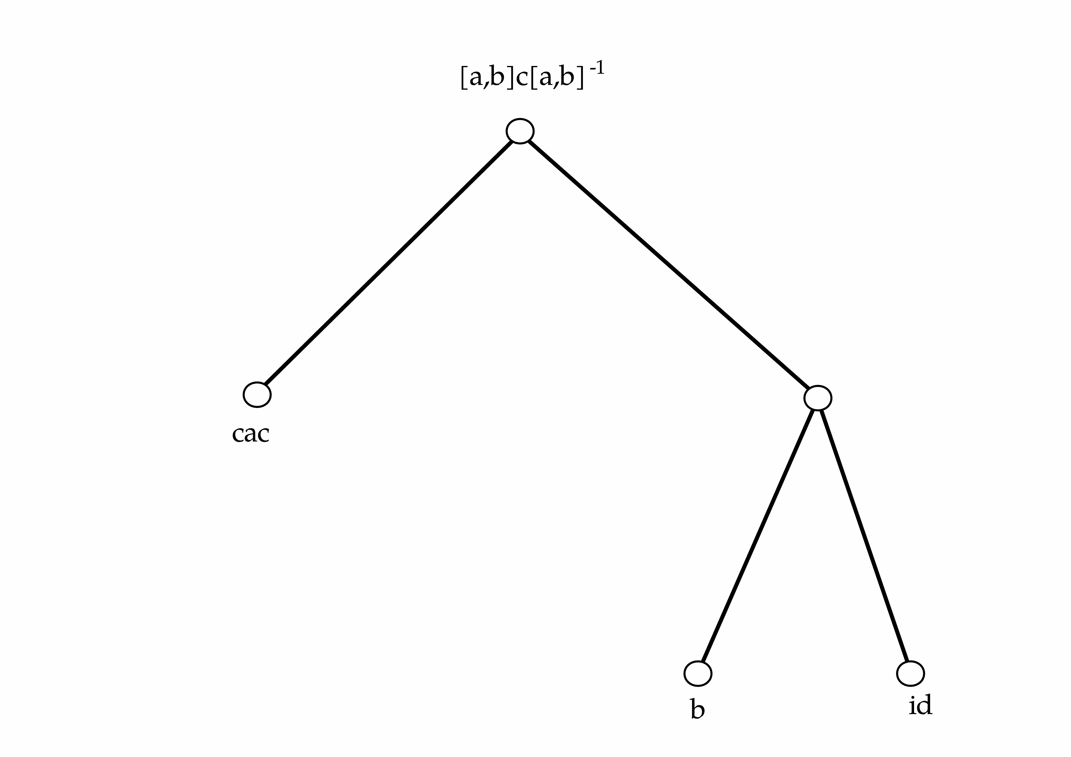
Figure 2.2. A portrait of $[a,b]c[a,b]^{-1}$ along $10$

Example 2.4.

Take in the first Grigorchuk group the element $g=[a,b]c[a,b]^{-1}$. Then the vertex $10$ is fixed by $g$. The portrait of $g$ along $10$ is given by $g_{0}=cac$, $g_{11}=id$ and $g_{10}=b$. See Figure 2.2.

3. Stabilization of germ configurations

The main purpose of this section is to formulate and prove Proposition 3.3 which provides a sufficient condition for stabilization of cosets of germ configurations.

We recall the notion of germs of homeomorphisms. Let $\mathcal{X}$ be a topological space. A germ of homeomorphism of $\mathcal{X}$ is an equivalence class of pairs $(g,x)$ where $x\in\mathcal{X}$ and $g$ is a homeomorphism between a neighborhood of $x$ and a neighborhood of $g(x)$; and two germs $(g_{1},x_{1})$ and $(g_{2},x_{2})$ are equal if $x_{1}=x_{2}$ and $g_{1},g_{2}$ coincide on a neighborhood of $x_{1}$. A composition $(g_{1},x_{1})(g_{2},x_{2})$ is defined if and only if $x_{1}\cdot g_{1}=x_{2}$. The inverse of the a germ $(g,x)$ is $(g,x)^{-1}=(g^{-1},x\cdot g)$. A groupoid of germs of homeomorphisms on $\mathcal{X}$ is a set of germs of homeomorphisms of $\mathcal{X}$ that is closed under composition and inverse, and that contains all identity germs $(id_{\mathcal{X}},x)$, $x\in\mathcal{X}$.

Let $G$ be a group acting by homeomorphisms on $\mathcal{X}$ from the right. Its groupoid of germs, denoted by $\mathcal{G}$, is the set of germs $\left\{(g,x):\ g\in G,x\in\mathcal{X}\right\}$. For $x\in\mathcal{X}$, the isotropy group of $\mathcal{G}$ at $x$, denoted by $\mathcal{G}_{x}$, is the set of germs $\left\{(g,x):\ g\in{\rm St}_{G}(x)\right\}$. In other words, $\mathcal{G}_{x}$ is the quotient of the stabilizer ${\rm St}_{G}(x)$ by the subgroup of $G$ which consists of elements acting trivially on a neighborhood of $x$.

Suppose there is a group $L$ acting by homeomorphisms on $\mathcal{X}$ such that for any point $x\in\mathcal{X}$, the orbits $x\cdot L=x\cdot G$ and the isotropy group $\mathcal{L}_{x}$ of its groupoid $\mathcal{L}$ is trivial. We refer to such an $L$ as an auxiliary group with trivial isotropy. Write conjugation of a germ $(g,x)\in\mathcal{G}_{x}$ by $\sigma\in L$ as

$$(g,x)^{\sigma}:=\left(\sigma^{-1}g\sigma,x\cdot\sigma\right)\in\mathcal{G}_{x\cdot\sigma}.$$

It’s easy to see that since $L$ has trivial isotropy groups, if $x\cdot\sigma_{1}=x\cdot\sigma_{2}$ for $\sigma_{1},\sigma_{2}\in L$, then $(g,x)^{\sigma_{1}}=(g,x)^{\sigma_{2}}$.

With the auxiliary group $L$ chosen, let $\hat{\mathcal{G}}$ be the groupoid of germs of the group $\left\langle G,L\right\rangle$. The isotropy group $\hat{\mathcal{G}}_{x}$ is called the group of germs in [Erschler04].

Notation 3.1.

Let $G\curvearrowright\mathcal{X}$ by homeomorphisms and $L$ be an auxiliary group with trivial isotropy. Suppose the isotropy group $\mathcal{\hat{G}}_{o}$ of $\hat{\mathcal{G}}$ is non-trivial at some point $o\in\mathcal{X}$. Let $H_{o}\lvertneqq\mathcal{\hat{G}}_{o}$ be a proper subgroup of $\mathcal{\hat{G}}_{o}$ . For each point $x\in o\cdot G$, fix a choice of $\sigma_{x}\in L$ such that $o\cdot\sigma_{x}=x$. Let

$$H_{x}:=\left\{(g,x)\in\mathcal{\hat{G}}_{x}:\ (\sigma_{x}g\sigma_{x}^{-1},o)\in H_{0}\right\},$$

then $H_{x}$ is a proper subgroup of $\hat{\mathcal{G}}_{x}$. Let $\mathcal{H}=\mathcal{H}(H_{o})$ be the following sub-groupoid of $\mathcal{G}$:

(3.1) $$\mathcal{H}:=\{(g,x):\ g\in G,\ x\in o\cdot G,\ (g\sigma^{-1},x)\in H_{x}\mbox{ where }\sigma\in L,\ x\cdot g=x\cdot\sigma\}.$$

We now discuss some examples of groupoid of germs of groups acting on rooted trees. Let $G<{\rm Aut}(\mathsf{T}_{\mathbf{d}})$, then $G$ acts on the boundary of the tree $\mathcal{X}=\partial\mathsf{T}_{\mathbf{d}}$ by homeomorphisms. Let $L$ be the subgroup of ${\rm Aut}(\mathsf{T}_{\mathbf{d}})$ that consists of all finitary automorphisms. In other words, an element $g\in{\rm Aut}(\mathsf{T}_{\mathbf{d}})$ is in $L$ if there exists a finite level $n$ such that all sections $g_{v}$ for $v\in\mathsf{L}_{n}$ are trivial. The group $L$ is locally finite. For $G<{\rm Aut}(\mathsf{T}_{\mathbf{d}})$, we use the group $L_{G}=\left\{\gamma\in L:\ x\cdot\gamma\in x\cdot G\mbox{ for all }x\in\partial\mathsf{T}\right\}$ as an auxiliary group with trivial isotropy groups. In particular if $G$ acts level transitively, then $L$ is used as the auxiliary group.

The isotropy groups of the groupoid of germs are easy to recognize in directed groups (called spinal groups in [BGShandbook, Chapter 2]).

Example 3.2.

Let $G_{\omega}$ be a Grigorchuk group and $o=1^{\infty}$. For any $\omega$, $G_{\omega}$ acts level transitively. Use the finitary automorphisms $L$ as the auxiliary group. From the definition of the group we have that if $x\notin o\cdot G_{\omega}$, that is $x$ is not cofinal with $1^{\infty}$, then the isotropy group $(\mathcal{G}_{\omega})_{x}$ is trivial.

For $\omega$ eventually constant, say eventually constant ${\bf 0}$, we have that $(d_{\omega},o)=(id,o)$ and $(b_{\omega},o)=(c_{\omega},o)$ in $(\mathcal{G}_{\omega})_{o}$. In this case for $x$ cofinal with $1^{\infty}$, $(\mathcal{G}_{\omega})_{x}\simeq\mathbb{Z}/2\mathbb{Z}$. For $\omega$ not eventually constant then $\left(\hat{\mathcal{G}}_{\omega}\right)_{x}=(\mathcal{G}_{\omega})_{x}=\{id,b,c,d\}$ for $x$ cofinal with $1^{\infty}$. In this case a group element $g$ has $\gamma$-germ at $x$, where $\gamma\in\{b,c,d\}$, if there is a finite level $n$ such that the section of $g$ at $x_{1}\ldots x_{n}$ is $\gamma_{\mathfrak{s}^{n}\omega}$.

When $\omega$ is not eventually constant, the subgroup $\left\langle b\right\rangle=\{id,b\}$ is a proper subgroup of $\hat{\mathcal{G}}_{o}$. We refer to the corresponding sub-groupoid $\mathcal{H}^{b}=\mathcal{H}(\left\langle b\right\rangle)$ of $\mathcal{G}$ as the groupoid of $\left\langle b\right\rangle$-germs. The groupoid of $\left\langle c\right\rangle$-germs ($\left\langle d\right\rangle$-germs resp.) is defined in the same way from the subgroup $\{id,c\}$ ($\{id,d\}$ resp.) of $\hat{\mathcal{G}}_{o}$.

Proposition 3.3 below provides a sufficient condition for stabilization of $\mathcal{H}$-cosets of germs based on the Green function of the induced random walk on the orbit. This criterion is applied to verify non-triviality of Poisson boundary for the measures with good control over tail decay constructed in Section 7 on Grigorchuk groups. Given a probability measure $\mu$ on $G$, its induced transition kernel $P_{\mu}$ on an orbit $o\cdot G$ is given by

$$P_{\mu}(x,y)=\sum_{g\in G}\mu(g)\mathbf{1}_{\{y=x\cdot g\}}.$$

The Green function $\mathbf{G}_{P_{\mu}}(x,y)$ of the $P_{\mu}$-random walk is

$$\mathbf{G}_{P_{\mu}}(x,y)=\sum_{n=0}^{\infty}P_{\mu}^{n}(x,y).$$

We refer to the book [WoessBook, Chapter I] for general background on random walks on graphs. In many situations, estimates on transition probabilities of the induced $P_{\mu}$-random walk are available while the $\mu$-random walk on the group $G$ is hard to understand.

Proposition 3.3.

Let $G$ be a countable group acting by homeomorphisms on $\mathcal{X}$ from the right and $L$ be an auxiliary group with trivial isotropy. Assume that the isotropy group $\mathcal{\hat{G}}_{o}$ is nontrivial at some point $o\in\mathcal{X}$ and $\hat{\mathcal{G}}_{o}=\mathcal{G}_{o}$.

Let $\mu$ be a non-degenerate probability measure on $G$. Let $P_{\mu}$ be the induced transition kernel on the orbit $o\cdot G$ and $\mathcal{\mathbf{G}}_{P_{\mu}}$ the Green function of the $P_{\mu}$-random walk. Suppose there exists a proper subgroup $H_{o}\lvertneqq\mathcal{\hat{G}}_{o}$ such that

(3.2) $$\sum_{x\in o\cdot G}\mathbf{G}_{P_{\mu}}(o,x)\mu\left(\left\{g\in G:\ (g,x)\notin\mathcal{H}\right\}\right)<\infty,$$

where $\mathcal{H}=\mathcal{H}(H_{0})$ is the sub-groupoid of $\mathcal{G}$ associated with $H_{o}$ defined in (3.1). Then the Poisson boundary of $(G,\mu)$ is non-trivial.

Remark 3.4.

Suppose $\mu$ have the following additional property: there exists a finite subset $V\subseteq o\cdot G$ such that for any element $g$ in the support of $\mu$, $(g,x)\in\mathcal{H}$ for all $x\notin V$, then the condition in Proposition 3.3 is equivalent to $G_{P_{\mu}}(o,o)<\infty$. In other words, the induced $P_{\mu}$-random walk is transient on the orbit $o\cdot G$. In this special case the claim is given by [Erschler04, Proposition 2]. For example, it can be applied to measures of the form $\mu=\frac{1}{2}(\nu+\eta)$, where $\nu$ is of finite support and for any element $g$ in the support of $\eta$, $(g,x)\in\mathcal{H}$ for all $x\in o\cdot G$. In this case we say $\eta$ is supported on a subgroup of restricted germs.

It is natural to consider $G$ as an embedded subgroup of the (unrestricted) permutational wreath product $\mathcal{\hat{G}}_{o}\wr\wr_{o\cdot G}G$ as follows.

Denote by $\mathcal{W}$ the semi-direct product $\left(\prod_{x\in o\cdot G}\mathcal{\hat{G}}_{x}\right)\rtimes G$. Record elements of $\mathcal{W}$ as pairs $\left(\Phi,g\right)$, where $g\in G$ and $\Phi$ assigns each point $x\in o\cdot G$ an element in the isotropy group $\mathcal{\hat{G}}_{x}$ at $x$. Denote by ${\rm supp}\Phi$ the set of points $x$ where $\Phi(x)$ is not equal to identity of $\mathcal{G}_{x}$. The action of $G$ on $\prod_{x\in o\cdot G}\mathcal{\hat{G}}_{x}$ is given by

$$(\tau_{g}\Phi)(x)=\sigma\Phi(x\cdot g)\sigma^{-1},$$

where $\sigma\in L$ satisfies $x\cdot\sigma=x\cdot g$. One readily checks that $\tau$ is a well-defined (doesn’t depend on the choice of $\sigma$) left action of $G$ on $\prod_{x\in o\cdot G}\mathcal{\hat{G}}_{x}$. Multiplication in $\mathcal{W}$ is given by $(\Phi,g)(\Phi^{\prime},g^{\prime})=\left(\Phi\tau_{g}\Phi^{\prime},gg^{\prime}\right)$. The semi-direct product $\mathcal{W}$ is isomorphic to the permutational wreath product $\mathcal{\hat{G}}_{x}\wr\wr_{o\cdot G}G$. We now describe an embedding $\vartheta:G\hookrightarrow\mathcal{W}$.

Fact 3.5.

Let $\vartheta:G\to\mathcal{W}$ by defined as $\vartheta(g)=(\Phi_{g},g)$ such that for $x\in o\cdot G$,

(3.3) $$\Phi_{g}(x)=(g\sigma^{-1},x)\in\mathcal{G}_{x},\ \mbox{where }\sigma\in L,\ x\cdot g=x\cdot\sigma.$$

Then $\vartheta$ is a monomorphism.

Proof.

Let $g_{1},g_{2}\in G$ and $\sigma_{1},\sigma_{2}\in L$ such that $x\cdot g_{1}=x\cdot\sigma_{1}$, $x\cdot g_{1}g_{2}=x\cdot g_{1}\sigma_{2}$. Then

$$\Phi_{g_{1}}(x)\left(\tau_{g_{1}}\Phi_{g_{2}}\right)(x) =(g_{1}\sigma_{1}^{-1},x)\left(g_{2}\sigma_{2}^{-1},x\cdot g_{1}\right)^{\sigma_{1}^{-1}}$$

$$=(g_{1}\sigma_{1}^{-1},x)(\sigma_{1}g_{2}\sigma_{2}^{-1}\sigma_{1}^{-1},x\cdot g_{1}\sigma_{1}^{-1})$$

$$=(g_{1}g_{2}\sigma_{2}^{-1}\sigma_{1}^{-1},x)=\Phi_{g_{1}g_{2}}(x).$$

It follows that $\vartheta$ is homomorphism. It is clearly injective.

∎

Proof of Proposition 3.3.

Let $X_{1},X_{2}\ldots$ be i.i.d. random variables on $G$, $W_{n}=X_{1}\ldots X_{n}$. Let $\vartheta:G\to\mathcal{W}$, $\vartheta(g)=(\Phi_{g},g)$, be the embedding as described in Fact 3.5. Along the random walk trajectory $W_{n}$, consider the $H_{o}$-coset of the germ at $o$. Denote by $\pi\left(\Phi_{W_{n}}(o)\right)$ the (right) coset of $\Phi_{W_{n}}(o)$ in $\mathcal{G}_{o}/H_{o}$. By the rule of multiplication in $\mathcal{W}$,

$$\Phi_{W_{n+1}}(o)=\Phi_{W_{n}}(o)\left(\Phi_{X_{n+1}}\left(o\cdot W_{n}\right)\right)^{\sigma_{n}^{-1}},\ \sigma_{n}\in L,\ o\cdot W_{n}=o\cdot\sigma_{n}.$$

Therefore the event

$$\left\{\pi\left(\Phi_{W_{n}}(o)\right)\neq\pi\left(\Phi_{W_{n+1}}(o)\right)\right\}=\left\{\Phi_{X_{n+1}}\left(o\cdot W_{n}\right)\notin H_{o\cdot W_{n}}\right\}.$$

By definition of the sub-groupoid of germs $\mathcal{H}$,

$$\left\{\Phi_{X_{n+1}}\left(o\cdot W_{n}\right)\notin H_{o\cdot W_{n}}\right\}=\left\{(X_{n+1},o\cdot W_{n})\notin\mathcal{H}\right\}.$$

Then

$$\sum_{n=0}^{\infty}\mathbb{P}\left(\pi\left(\Phi_{W_{n}}(o)\right)\neq\pi\left(\Phi_{W_{n+1}}(o)\right)\right) =\sum_{n=0}^{\infty}\mathbb{P}\left((X_{n+1},o\cdot W_{n})\notin\mathcal{H}\right)$$

$$=\sum_{n=0}^{\infty}\sum_{x\in o\cdot G}\sum_{g\in G}\mu(g)\mathbf{1}_{\{(g,x)\notin\mathcal{H}\}}\mathbb{P}\left(x=o\cdot W_{n}\right)$$

$$=\sum_{x\in o\cdot G}{\bf G}_{P_{\mu}}(o,x)\mu\left(\left\{g:\ (g,x)\notin\mathcal{H}\right\}\right).$$

If the summation is finite, by the Borel-Cantelli lemma, $\pi\left(\Phi_{W_{n}}(o)\right)$ stabilizes a.s. along the random walk trajectory $\left(W_{n}\right)$. For each coset $\gamma H_{o}$ in $\hat{\mathcal{G}}_{o}/H_{o}$, consider the tail event

$$A_{\gamma H_{o}}=\left\{\lim_{n\to\infty}\pi\left(\Phi_{W_{n}}(o)\right)=\gamma H_{o}\right\}.$$

Given $\gamma\in\hat{\mathcal{G}}_{o}=\mathcal{G}_{o}$, let $g\in G$ be a group element such that $o\cdot g=o$ and $\Phi_{g}(o)=\gamma$. Note that $\mathbb{P}_{id}\left(A_{H_{o}}\right)=\mathbb{P}_{g}\left(A_{\gamma H_{o}}\right)$ and for any $m\in\mathbb{N}$,

$$\mathbb{P}_{id}\left(A_{H_{o}}\right)=\mathbb{P}_{g}\left(A_{\gamma H_{o}}\right) \geq\mu^{(m)}(g^{-1})\mathbb{P}_{id}\left(A_{\gamma H_{o}}\right),$$

$$\mathbb{P}_{id}\left(A_{\gamma H_{o}}\right) \geq\mu^{(m)}(g)\mathbb{P}_{g}\left(A_{\gamma H_{o}}\right)=\mu^{(m)}(g)\mathbb{P}_{id}\left(A_{H_{o}}\right).$$

Since $\mu$ is non-degenerate, there exists a finite $m$ such that $\mu^{(m)}(g),\mu^{(m)}(g^{-1})>0$. Then $\mathbb{P}_{id}\left(A_{H_{o}}\right)=0$ would imply $\mathbb{P}_{id}\left(A_{\gamma H_{o}}\right)=0$ for all $\gamma\in\mathcal{G}_{o}$. On the other hand since $\pi\left(\Phi_{W_{n}}(o)\right)$ stabilizes with probability $1$, we have $\mathbb{P}_{id}\left(\cup_{\gamma H_{o}\in\mathcal{G}_{o}/H_{o}}A_{\gamma H_{o}}\right)=1$. It follows that $\mathbb{P}_{id}\left(A_{H_{o}}\right)>0$. Since $\mathbb{P}_{id}\left(A_{\gamma H_{o}}\right)\geq\mu^{(m)}(g)\mathbb{P}_{id}\left(A_{H_{o}}\right)>0$, it follows that $\mathbb{P}_{id}\left(A_{H_{0}}\right)<1$. We conclude that $A_{H_{o}}$ is a non-trivial tail event and the Poisson boundary of $(G,\mu)$ is non-trivial.

∎

The boundary behavior of random walk in Proposition 3.3 can be viewed as a lamplighter boundary. Under the embedding $\vartheta:g\mapsto(\Phi_{g},g)$, we refer to $\Phi_{g}$ as the germ configuration of $g$. Let $(W_{n})$ be a random walk on $G$ with a non-degenerate step distribution $\mu$. If (3.2) holds, then for every point $x\in o\cdot G$, the coset of $\Phi_{W_{n}}(x)$ in $\mathcal{\hat{G}}_{x}/H_{x}$ stabilizes with probability one along an infinite trajectory of the random walk $(W_{n})$. Thus if we view $\prod_{x}\mathcal{\hat{G}}_{x}/H_{x}$ as the space of germ configurations mod $\prod_{x}H_{x}$, then when stabilization occurs, we have a limit configuration $\Phi_{W_{\infty}}$ in this space of cosets. Endowed with the hitting distribution, it can be viewed as a $\mu$-boundary.

4. measures with nontrivial Poisson boundaries on the first Grigorchuk group

In this section, we give quick examples of non-degenerate symmetric probability measures on the first Grigorchuk group with non-trivial Poisson boundary. Choices of such measures with better quantitative control over the tail decay will be discussed in Section 6 and Section 7.

Recall that the first Grigorchuk group $G=G_{012}$ acts on the rooted binary tree, and it is generated by $\{a,b,c,d\}$ where

$$a=(1,1)\varepsilon,\ b=(a,c),\ c=(a,d),\ d=(1,b).$$

As explained in Example 3.2, the generators $b,c,d$ have nontrivial germs at $o=1^{\infty}$. The isotropy group of $\mathcal{G}$ at $o$ is $\mathcal{G}_{o}\simeq\left(\mathbb{Z}/2\mathbb{Z}\right)\times\left(\mathbb{Z}/2\mathbb{Z}\right)$. List the elements of $\mathcal{G}_{o}$ as $\left\{id,b,c,d\right\}$, where $b$ stands for the germ $(b,o)$, similarly $c$ and $d$ stand for the corresponding germs. Take the following proper subgroup of $\mathcal{G}_{o}$:

$$H_{o}=\{id,b\}.$$

The group $L$ of finitary automorphisms of the rooted binary tree plays the role of the auxiliary group. Recall the definition of the sub-groupoid $\mathcal{H}^{b}=\mathcal{H}(H_{o})$ as in (3.1), which we will refer to as the sub-groupoid of $b$-germs. Now consider the subgroup $\mathrm{H}^{b}<G$ which consists of group elements that only have trivial or $b$-germs, that is

(4.1) $$\mathrm{H}^{b}=\{g\in G:\ (g,x)\in\mathcal{H}^{b}\ \mbox{for all }x\in 1^{\infty}\cdot G\}.$$

Given an element in $G$, one can recognize whether it is in ${\rm H}^{b}$ from its sections in a deep enough level.

Fact 4.1.

Let $g\in G$ be a group element. Then $g\in\mathrm{H}^{b}$ if and only if there exists $k\in\mathbb{N}$ such that the section $g_{v}$ is in the set $\{id,a,b\}$ for all $v\in\mathsf{L}_{3k}$.

Proof.

The “if” direction follows from definition of $\mathrm{H}^{b}$.

We show the only if direction. Since $G$ is contracting, for any $g\in G$, there exists a finite level $n$ such that all sections $g_{v}$, $v\in\mathsf{L}_{n}$, are in the nucleus $\mathcal{N}=\{id,a,b,c,d\}$, see [NekraBook, Section 2.11]. Perform the wreath recursion down further $1$ or $2$ levels such that $n\equiv 0\ \mod 3$. Suppose on the contrary there exists a vertex $v\in\mathsf{L}_{n}$ such that the section is $c$ or $d$. Then $(g,v1^{\infty})$ is a $c$-germ or $d$-germ, a contradiction with $g\in{\rm H}^{b}$. Thus the level $n$ satisfies the condition in the statement.

∎

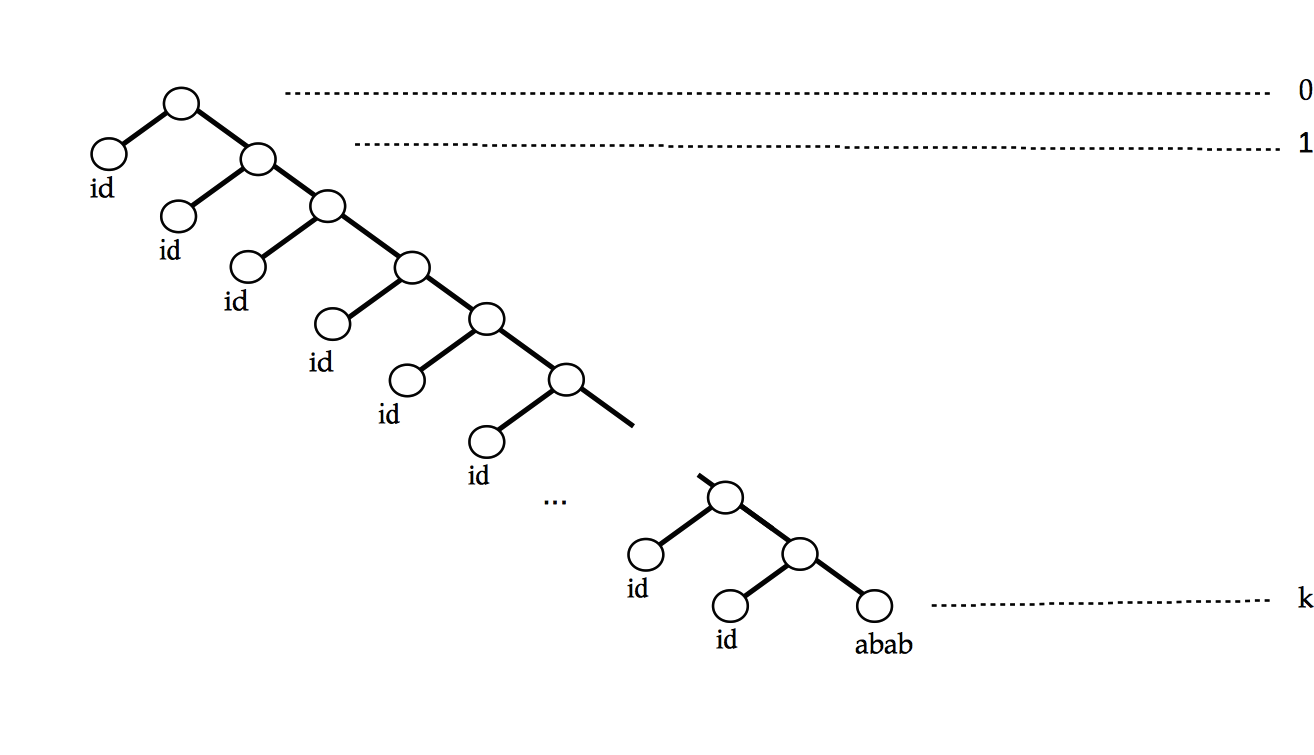
Figure 4.1. Portrtrait of $\sigma^{k}(abab)$ in the first Grigorchuk group in usual notation. If $k$ is divisible by $3$, then the element belongs to $\rm{H}^{b}$ (the group with germs equal to the germ of $b$ or trivial.)

A key property we will use is that the orbit of $1^{\infty}$ under the action of ${\rm H}^{b}$ is infinite. Recall the notation $\iota(g,u)$ as defined in (2.1), which denotes the automorphism in the rigid stabilizer of $u$ that acts as $g$ in the subtree rooted at $u$. Note that for any $n\in\mathbb{N}$, $\iota([a,b],1^{n})\in G$. Explicitly we have $\iota([a,b]:1^{n})=\sigma^{n}(abab)$ where $\sigma$ is the homomorphism given by substitution $a\mapsto cac,b\mapsto d,c\mapsto b,d\mapsto c$. More generally, $\iota(g,u)\in G$ for any $g\in K=\left\langle\left[a,b\right]\right\rangle^{G}$ and any vertex $u\in\mathsf{T}$, because $G$ is regularly branching over the subgroup $K$, see [BGShandbook, Proposition 1.25]. The portrait of $\iota\left([a,b],1^{k}\right)$ is drawn in Figure 4.1. The subset $\{\iota\left([a,b],1^{3k}\right)$: $k\geq 0\}$ is contained in ${\rm H}^{b}$. Since $1^{\infty}\cdot[a,b]=1001^{\infty}$, it follows that

$$1^{\infty}\cdot\iota\left([a,b],1^{3k}\right)=1^{3k+1}001^{\infty}.$$

Therefore the orbit $1^{\infty}\cdot{\rm H}^{b}$ is infinite.

By Proposition 3.3 and Remark 3.4 we can take a measure with non-trivial Poisson boundary of the form $\mu=\frac{1}{2}(\nu+\eta)$, where $\mbox{supp}\nu=\{a,b,c,d\}$ and $\eta$ is a symmetric measure supported on ${\rm H}^{b}$ with transient induced random walk on the orbit $1^{\infty}\cdot{\rm H}^{b}$. Existence of such a measure $\eta$ is deduced from the fact that the orbit $1^{\infty}\cdot{\rm H}^{b}$ is infinite by the following lemma. It is [Erschler04, Lemma 7.1] with the assumption of $A$ being finitely generated dropped. Since the subgroup ${\rm H}^{b}$ is not finitely generated, we include a proof of the lemma. Let $A$ be a countable group and $B$ a subgroup of $A$. Given a probability measure $\eta$ on $A$, recall that the induced transition kernel $P_{\eta}$ on the (left) cosets of $B$ is

$$P_{\eta}(Bx,By)=\sum_{g\in A}\eta(g)\mathbf{1}_{\{Bxg=By\}},$$

where $x,y\in A$ and $Bx,By$ are cosets of $B$. We say the measure $\eta$ is transient with respect to $B$ if ${\bf G}_{P_{\eta}}(B,B)=\sum_{n=0}^{\infty}P_{\eta}^{n}(B,B)<\infty$.

Lemma 4.2.

Let $A$ be a countable group and $B<A$ a subgroup of infinite index. Then there exists a non-degenerate symmetric probability measure $\eta$ on $A$ that is transient with respect to $B$.

Apply Lemma 4.2 to the group ${\rm H}^{b}$ and its subgroup ${\rm H}^{b}\cap{\rm St}_{G}(1^{\infty})$. Since the orbit $1^{\infty}\cdot{\rm H}^{b}$ is infinite, there is a symmetric measure $\eta$ on ${\rm H}^{b}$ such that the induced random walk $P_{\eta}$ on $1^{\infty}\cdot{\rm H}^{b}$ is transient. Let ${\bf u}_{S}$ be uniform on the generating set $S=\{a,b,c,d\}$ and take $\mu=\frac{1}{2}({\bf u}_{S}+\eta)$. Since obviously the Dirichlet forms of $P_{\mu}$ and $P_{\eta}$ satisfy $\mathcal{E}_{P_{\mu}}\geq\frac{1}{2}\mathcal{E}_{P_{\eta}}$, by comparison principle (see for example [WoessBook, Corollary 2.14]), the induced random walk $P_{\mu}$ on $1^{\infty}\cdot G$ is transient as well. Since $\eta$ is supported on the subgroup ${\rm H}^{b}$ with only $b$-germs and $\nu$ is of finite support, as explained in Remark 3.4, transience of $P_{\mu}$ verifies the condition (3.2) in Proposition 3.3. We conclude that $(G,\mu)$ has non-trivial Poisson boundary.

Proof of Lemma 4.2.

First take a symmetric measure $\mu$ on $A$ such that $\mu(id)=\frac{1}{2}$ and the support of $\mu$ generates the group $A$. The induced random walk $P_{\mu}$ on the cosets $B\setminus A$ is irreducible since ${\rm supp}\mu$ generates $A$. Since $B\setminus A$ is infinite, $P_{\mu}$ admits no non-zero invariant vector in $\ell^{2}(B\setminus A)$, therefore

$$P_{\mu}^{n}(B,B)\searrow 0\ \mbox{as }n\to\infty.$$

Indeed, denote by $E_{s}^{I-P_{\mu}}$ the spectral resolution of $I-P_{\mu},$

$$I-P_{\mu}=\int_{0}^{1}sdE_{s}^{I-P_{\mu}}.$$

Write $N(s)=\left\langle E_{s}^{I-P_{\mu}}\mathbf{1}_{B},\mathbf{1}_{B}\right\rangle$Then $P_{\mu}^{n}(B,B)=\int_{0}^{1}(1-s)^{n}dN(s)$. Since $(I-P_{\mu})f=0$ has no solution in $\ell^{2}(B\setminus A)$, we have that $N(0)=0$. Thus $P_{\mu}^{n}(B,B)\searrow 0\ \mbox{as }n\to\infty$.

Next we show that if $P_{\mu}^{n}(B,B)\to 0$ as $n\to\infty$, then some convex linear combinations of convolution powers of $\mu$, that is measures of the form

$$\eta=\sum_{n=1}^{\infty}c_{n}\mu^{(n)},\ \sum_{n=1}^{\infty}c_{n}=1,\ c_{n}\geq 0,$$

induce transient random walks on $B\setminus A$. Following [BSC], we call $\eta$ a discrete subordination of $\mu$. Let $\psi$ be a smooth strictly increasing function on $(0,\infty)$ such that $\psi(0)=0$, $\psi(1)=1$. Suppose that we have expansion $\psi(1-s)=1-\sum_{n=1}^{\infty}c_{n}s^{n}$ for $|s|\leq 1$ with coefficients $c_{n}\geq 0$. Then one can take

$$\mu_{\psi}:=I-\psi(I-\mu)=\sum_{n=1}^{\infty}c_{n}\mu^{(n)}.$$

The class of functions $\psi$ that are suitable for this operation is the Bernstein functions, see the book [SSVbook].

The induced random walk transition operator $P_{\mu}$ is a self-adjoint operator acting on $\ell^{2}(B\setminus A)$. Recall that $E_{s}^{I-P_{\mu}}$ denotes the spectral resolution of $I-P_{\mu},$then we have

$$I-P_{\mu_{\psi}}=\psi\left(I-P_{\mu}\right)=\int_{0}^{1}\psi(s)dE_{s}^{I-P_{\mu}}.$$

It follows that

$$P_{\mu_{\psi}}^{2n}(B,B)=\int_{0}^{1}(1-\psi(s))^{2n}d\left\langle E_{s}^{I-P_{\mu}}\mathbf{1}_{B},\mathbf{1}_{B}\right\rangle.$$

Since there is no non-zero $P_{\mu}$-invariant vector in $\ell^{2}(B\setminus A)$, $N(s)\to 0$ as $s\to 0+$. Since

$$\sum_{n=0}^{\infty}P_{\mu_{\psi}}^{2n}(B,B)=\sum_{n=0}^{\infty}\int_{0}^{1}(1-\psi(s))^{2n}dN(s)=\int_{0}^{1}s^{-1}dN\circ\psi^{-1}(s),$$

to make the Green function finite, it suffices to take some $\psi$ such that $N\circ\psi^{-1}(s)\leq cs^{1+\epsilon}$ for some $\epsilon>0$ near $0$. For example one can take the measure $\nu$ on $(0,\infty)$ such that

$$\nu((x,\infty))=N(1/x)^{\frac{1}{1+\epsilon}},\ x\geq 1,$$

and $\psi$ to be the Bernstein function with representing measure $\nu$, $\psi(s)=\int_{(0,\infty)}(1-e^{-st})\nu(dt)$. Note that the coefficients $c_{n}$ in the expansion $\psi(1-s)=1-\sum_{n=1}^{\infty}c_{n}s^{n}$ are positive. We conclude that for this choice the $P_{\mu_{\psi}}$-random walk on $B\setminus A$ is transient.

∎

The measure $\eta$ in Lemma 4.2 with transient induced random walk on the orbit of $o$ is obtained from discrete subordination of some non-degenerate measure on ${\rm H}^{b}$. We wish to point out that in general, the measure $\eta$ does not necessarily have finite entropy. In Section 5, we develop a direct method to construct measures with transient induced random walks such that the resulting measures have finite entropy and explicit tail decay bounds. Unlike the general Lemma 4.2, this construction heavily relies on the structure of the groups under consideration. This will be crucial in applications to growth estimates.

5. Further construction of measures with transient induced random walk

5.1. Measures constructed from cube independent elements

In this subsection we describe a construction of measures with transient induced random walks. It is particularly useful in groups acting by homeomorphisms possessing a rich collection of rigid stabilizers. Transience of the induced random walk is deduced from $\ell^{2}$-isoperimetric inequalities.

Let $P$ be a transition kernel on a countable graph $X$. We assume that $P$ is reversible with respect to $\pi$, that is $\pi(x)P(x,y)=\pi(y)P(y,x)$. The Dirichlet form of $P$ is defined by

$$\mathcal{E}_{P}(f)=\frac{1}{2}\sum_{x,y\in X}(f(x)-f(y))^{2}P(x,y)\pi(x).$$

Denote by $\left\|f\right\|_{\ell^{2}(\pi)}$ the $\ell^{2}$-norm of $f$ with respect to the measure $\pi$. Given a finite subset $\Omega\subset X$, denote by $\lambda_{1}(\Omega)$ the smallest Dirichlet eigenvalue:

$$\lambda_{1}(\Omega)=\inf\left\{\mathcal{E}_{P}(f):\ {\rm supp}f\subseteq\Omega,\ \left\|f\right\|_{\ell^{2}(\pi)}=1\right\}.$$

An inequality of the form $\lambda_{1}(\Omega)\geq\Lambda(\pi(\Omega))$ is referred to as an $\ell^{2}$-isoperimetric inequality. It is also known as a Faber-Krahn inequality.

The following isoperimetric test for transience is from [grigoryanAG, Theorem 6.12]. It is a consequence of the connection between $\ell^{2}$-isoperimetric inequalities and on-diagonal heat kernel upper bound, see Coulhon [coulhon, Proposition V.1] or Grigor’yan [grigoryan].

Proposition 5.1 (Isoperimetric test for transience [grigoryanAG]).

Suppose $v_{0}=\inf_{x\in X}\pi(x)>0$. Assume that

$$\lambda_{1}(\Omega)\geq\Lambda(\pi(\Omega))$$

holds for all finite non-empty subset $\Omega\subset X$, where $\Lambda$ is a continuous positive decreasing function on $[v_{0},\infty)$. If

$$\int_{v_{0}}^{\infty}\frac{ds}{s^{2}\Lambda(s)}<\infty,$$

then the Markov chain $P$ on $X$ is transient.

The best possible choice of the function $\Lambda$ is defined as the $\ell^{2}$-isoperimetric profile $\Lambda_{P}$ of $P$,

$$\Lambda_{P}(v):=\inf\left\{\lambda_{1}(\Omega):\ \Omega\subset X\mbox{ and }\pi(\Omega)\leq v\right\}.$$

A useful way to obtain lower bounds on $\Lambda_{P}$ is through $\ell^{1}$-isoperimetry. By Cheeger’s inequality (see [LS, Theorem 3.1])

(5.1) $$\lambda_{1}(\Omega)\geq\frac{1}{2}\left(\frac{\left|\partial_{P}\Omega\right|}{\pi(\Omega)}\right)^{2},$$

where $\left|\partial_{P}\Omega\right|=\sum_{x\in\Omega,y\in\Omega^{c}}\pi(x)P(x,y)$ is the size of the boundary of $\Omega$ with respect to $(P,\pi)$.

In what follows we will consider $P_{\mu}$ on $X$ induced by a symmetric probability measure $\mu$ on $G$, $G\curvearrowright X$. In this case $P_{\mu}$ is symmetric and reversible with respect to $\pi\equiv 1$.

Lemma 5.2.

Let $G$ be a countable group acting on $X$, $o\in X$ be a point such that the orbit $o\cdot G$ is infinite. Suppose there is a sequence of finite subsets $F_{n}\subseteq G$ with $|F_{n}|\nearrow\infty$ as $n\to\infty$ and a constant $c_{0}>0$ such that

$$\inf_{x\in o\cdot G}\left|x\cdot F_{n}\right|\geq c_{0}|F_{n}|.$$

Let $(\lambda_{n})$ be a sequence of positive numbers such that $\sum_{n=1}^{\infty}\lambda_{n}=1$ and

$$\sum_{n=1}^{\infty}\frac{1}{\lambda_{n}\left(|F_{n}|-|F_{n-1}|\right)}<\infty.$$

Let

$$\mu=\sum_{n=1}^{\infty}\frac{\lambda_{n}}{2}\left(\mathbf{u}_{F_{n}}+\mathbf{u}_{F_{n}^{-1}}\right),$$

where $\mathbf{u}_{F}$ denotes the uniform measure on the set $F$. Then the induced $P_{\mu}$-random walk on $o\cdot G$ is transient.

Proof.

Denote by $P_{n}$ the transition kernel on $o\cdot G$ induced by the measure $\frac{1}{2}\left(\mathbf{u}_{F_{n}}+\mathbf{u}_{F_{n}^{-1}}\right)$. Under the assumption that $\inf_{x\in o\cdot H}\left|x\cdot F_{n}\right|\geq c_{0}|F_{n}|$, we have that for any set $U\subset o\cdot G$ with $|U|\leq\frac{c_{0}}{2}|F_{n}|$,

$$\frac{|\partial_{P_{n}}U|}{|U|}\geq\frac{c_{0}}{4}.$$

Indeed, the size of the boundary is given by

$$|\partial_{P_{n}}U|=\sum_{x\in U,y\in U^{c}}P_{n}(x,y)=\sum_{x\in U}\frac{1}{|F_{n}|}\sum_{g\in F_{n}}\frac{1}{2}\left(\mathbf{1}_{U^{c}}(x\cdot g)+\mathbf{1}_{U^{c}}(x\cdot g^{-1})\right).$$

The assumption that $\inf_{x\in o\cdot H}\left|\{x\cdot F_{n}\}\right|\geq c_{0}|F_{n}|$ implies that for any $x$,

$$\sum_{g\in F_{n}}\mathbf{1}_{U^{c}}(x\cdot g)=|x\cdot F_{n}|-\sum_{g\in F_{n}}\mathbf{1}_{U}(x\cdot g)\geq c_{0}|F_{n}|-|U|.$$

It follows that for $|U|\leq\frac{c_{0}}{2}|F_{n}|$,

$$\frac{|\partial_{P_{n}}U|}{|U|}\geq\frac{1}{2}\frac{c_{0}|F_{n}|-|U|}{|F_{0}|}\geq\frac{c_{0}}{4}.$$

We mention that the argument above is well-known, it is a step in the proof of the Coulhon-Saloff-Coste isoperimetric inequality [csc].

By Cheeger’s inequality (5.1), the $\ell^{2}$-isoperimetric profile of $P_{n}$ satisfies

$$\Lambda_{P_{n}}(v)\geq\frac{1}{2}\left(\frac{c_{0}}{4}\right)^{2}\mbox{ for all }v\leq\frac{c_{0}}{2}|F_{n}|.$$

Now the random walk induced by $\mu$ is the convex linear combination $P_{\mu}=\sum_{n=1}^{\infty}\lambda_{n}P_{n}$. By definition it is clear that $\mathcal{E}_{P_{\mu}}\geq\lambda_{n}\mathcal{E}_{P_{n}}$. Therefore we have a piecewise lower bound on $\Lambda_{P_{\mu}}$:

$$\Lambda_{P_{\mu}}(v)\geq\frac{1}{2}\left(\frac{c_{0}}{4}\right)^{2}\lambda_{n}\ \ \mbox{for }v\in\left(\frac{c_{0}}{2}|F_{n-1}|,\frac{c_{0}}{2}|F_{n}|\right],n\in\mathbb{N}.$$

Plug the estimate into the isoperimetric test for transience, we have

$$\int_{1}^{\infty}\frac{ds}{s^{2}\Lambda_{P_{\mu}}(s)}\leq C\sum_{n=1}^{\infty}\frac{1}{\lambda_{n}(|F_{n}|-|F_{n-1}|)}.$$

If the summation on the right hand side of the inequality is finite, then by Proposition 5.1, the induced random walk $P_{\mu}$ is transient.

∎

Example 5.3.

Suppose there is a sequence of $F_{n}$ satisfying the assumption of Lemma 5.2 with volume $|F_{n}|\sim\theta^{n}$. Then one can choose the sequence $(\lambda_{n})$ to be $\lambda_{n}=C_{\epsilon}\theta^{-n}n^{1+\epsilon}$ for any $\epsilon>0$. The resulting convex linear combination $\mu$ as in the statement of the lemma induces transient random walk on the orbit of $o$.

The condition in Lemma 5.2 forces $F_{n}\cap{\rm St}_{G}(x)$ to be small for all $x$ in the orbit. Such sets are not common to observe, especially in the situation of totally non-free actions. In applications to Grigorchuk groups, the subsets $F_{n}$ are built from a sequence of elements which satisfy an injective property which we refer to as "cube independence" defined below. We have mentioned the definition of cube independence property for ${\bf k}=1$ in the Introduction, now we formulate a more general definition.

For a sequence of elements $g_{1},g_{2},\ldots\in G$, we say the sequence satisfies the cube independence property on $x_{0}\cdot G$ with parameters $\mathbf{k}=\left(k_{n}\right){}_{n=1}^{\infty}$, $k_{n}\in\mathbb{N}$, if for any $n\geq 1$ and $x\in x_{0}\cdot G$, the map

$$\{0,1,\ldots,k_{1}\}\times\ldots\times\{0,1,\ldots,k_{n}\} \to x_{0}\cdot G$$

$$(\varepsilon_{1},\ldots\varepsilon_{n}) \mapsto x\cdot g_{n}^{\varepsilon_{n}}\ldots g_{1}^{\varepsilon_{1}}$$

is injective. When the parameters $k_{n}$ are constant $1$, we omit reference to $\mathbf{k}$ and say the sequence has the cube independence property.

Any other ordering of the elements $g_{1},\ldots,g_{n}$ in the definition would serve the same purpose, but we choose to formulate it this way because in examples we consider it is easier to verify inductively. By definition it is clear that cube independence property is inherited by subsequences.

Proposition 5.4.

Suppose $g_{1},g_{2},\ldots\in G$ is a sequence of elements satisfying the cube independence property on the orbit $x_{0}\cdot G$ with $\mathbf{k}=(k_{n})$, $k_{n}\in\mathbb{N}$. Let

$$F_{n}=\left\{g_{n}^{\varepsilon_{n}}\ldots g_{1}^{\varepsilon_{1}}:\ \varepsilon_{j}\in\{0,1,\ldots,k_{j}\},1\leq j\leq n\right\}.$$

For any $\epsilon>0$, let

$$\mu=\sum_{n}\frac{C_{\epsilon}n^{1+\epsilon}}{2(1+k_{1})\ldots(1+k_{n})}\left(\mathbf{u}_{F_{n}}+\mathbf{u}_{F_{n}^{-1}}\right),$$

where $C_{\epsilon}$ is the normalizing constant such that $\mu$ has total mass $1$. Then $\mu$ is a symmetric probability measure on $G$ of finite entropy such that the induced $P_{\mu}$-random walk on $x_{0}\cdot G$ is transient.

Proof.

By definition of cube independence property, we have for all $x\in x_{0}\cdot G$, $|x\cdot F_{n}|=|F_{n}|=\prod_{j=1}^{n}(1+k_{j})$. Choose $\lambda_{n}=C_{\epsilon}n^{1+\epsilon}\prod_{j=1}^{n}(1+k_{j})^{-1}$, then

$$\sum_{n=1}^{\infty}\frac{1}{\lambda_{n}\left(|F_{n}|-|F_{n-1}|\right)}\leq 2\sum_{n=1}^{\infty}\frac{1}{\lambda_{n}|F_{n}|}=\frac{2}{C_{\epsilon}}\sum_{n=1}^{\infty}n^{-1-\epsilon}<\infty.$$

Therefore by Lemma 5.2, the convex combination $\mu=\sum_{n=1}^{\infty}\frac{\lambda_{n}}{2}\left(\mathbf{u}_{F_{n}}+\mathbf{u}_{F_{n}^{-1}}\right)$ induces transient random walk on the orbit $o\cdot G$. The entropy of $\mu$ is bounded by

$$H_{\mu}(1) \leq\sum_{n=1}^{\infty}\lambda_{n}\log|F_{n}|$$

$$=C\sum_{n=1}^{\infty}\frac{n^{1+\epsilon}}{\prod_{j=1}^{n}(1+k_{j})}\log\left(\prod_{j=1}^{n}(1+k_{j})\right)<\infty,$$

where the series is summable because $\prod_{j=1}^{n}(1+k_{j})\geq 2^{n}$.

∎

Remark 5.5.

As mentioned in the Introduction, we refer to the set $F_{n}$ as an $n$-quasi-cubic set and the measure ${\bf u}_{F_{n}}$ an $n$-quasi-cubic measure. By definition bounds on the length of elements $g_{1},g_{2},\ldots$ give explicit estimates of the truncated moments and tail decay of $\mu$. More precisely, if $\sum_{j=1}^{n}(1+k_{j})|g_{j}|\leq\ell_{n}$, then $\max\{|g|,\ g\in F_{n}\}\leq\ell_{n}$ and for the measure $\mu$ in Corollary 5.4,

$$\mu\left(B(e,\ell_{n})^{c}\right)\leq\frac{C^{\prime}_{\epsilon}n^{1+\epsilon}}{(1+k_{1})\ldots(1+k_{n})}.$$

One way to produce a cube independent sequence is to select suitable elements from level stabilizers.

Lemma 5.6.

Let $G<{\rm Aut}(\mathsf{T}_{d})$ and suppose that $g_{n}\in G$ satisfies that $g_{n}\in{\rm St}_{G}(\mathsf{L}_{n})$ and the root permutation of the section $(g_{n})_{v}$ has no fixed point for all $v\in\mathsf{L}_{n}$. Then the sequence $(g_{n})_{n\geq 0}$ has the cube independence property on $1^{\infty}\cdot G$.

Proof.

Given $x\in 1^{\infty}\cdot G$, we need to show injectivity of the map

$$\{0,1\}^{n} \to 1^{\infty}\cdot G$$

$$(\varepsilon_{1},\ldots\varepsilon_{n}) \mapsto x\cdot g_{n}^{\varepsilon_{n}}\ldots g_{1}^{\varepsilon_{1}}.$$

Since $\left\langle g_{2},\ldots,g_{n}\right\rangle$ is in the stabilizer of level $2$, we have that the first two digits of $y=x\cdot g_{n}^{\varepsilon_{n}}\ldots g_{1}^{\varepsilon_{1}}$ is $x_{1}x_{2}\cdot g_{1}^{\epsilon}$. Combined with the assumption on the root permutation of $(g_{1})_{v}$, $v\in\mathsf{L}_{1}$, the second digit of $y$ is different from $x_{2}$ if and only if $\varepsilon_{1}=1$. Thus $x\cdot g_{n}^{\varepsilon_{n}}\ldots g_{1}^{\varepsilon_{1}}=x\cdot g_{n}^{\varepsilon^{\prime}_{n}}\ldots g_{1}^{\varepsilon^{\prime}_{1}}$ implies $\varepsilon_{1}=\varepsilon_{1}^{\prime}$. The same argument recursively shows that $\varepsilon_{j}=\varepsilon_{j}^{\prime}$ for all $1\leq j\leq n$.

∎

5.2. Critical constant of recurrence

In this subsection we consider an explicit sequence of cube independent elements on the first Grigorchuk group $G$, obtained by applying certain substitutions. As an application of Proposition 5.4, we evaluate the critical constant for recurrence of $(G,{\rm St}_{G}(1^{\infty}))$.

The notion of critical constant for recurrence of $(G,H)$, where $H$ is a subgroup of $G$, is introduced in [Erschler05]. For a group $G$ equipped with a length function $l$ and a subgroup $H<G$ of infinite index, the critical constant for recurrence $c_{{\rm rt}}(G,H)$ with respect to $l$, is defined as $\sup\beta$, where the $\sup$ taken is over all $\beta\geq 0$ such that there exists a symmetric probability measure $\mu$ on $G$ with transient induced random walk on $H\setminus G$ and $\mu$ has finite $\beta$-moment with respect to $l$ on $G$:

$$\sum_{g\in G}l(g)^{\beta}\mu(g)<\infty.$$

When $G$ is finitely generated and $l$ is the word distance on a Cayley graph of $G$, we omit reference to $l$.

For the rest of this subsection, $G$ denotes the first Grigorchuk group $G_{012}$ and we use the usual notation for $G$ as in (2.4). By [Erschler05, Theorem 2], for $H$ the stabilizer ${\rm St}_{G}(1^{\infty})$, the critical constant $c_{{\rm rt}}(G,{\rm St}_{G}(1^{\infty}))<1$. We show that indeed $c_{{\rm rt}}\left(G,{\rm St}_{G}(1^{\infty})\right)$ is equal to the growth exponent of the permutational wreath product $(\mathbb{Z}/2\mathbb{Z})\wr_{\mathcal{S}}G$, $\mathcal{S}=1^{\infty}\cdot G$.

Theorem 5.7.

Let $G$ be the first Grigorchuk group. Then

$$c_{{\rm rt}}\left(G,{\rm St}_{G}(1^{\infty})\right)=\alpha_{0}=\frac{\log 2}{\log\lambda_{0}},$$

where $\lambda_{0}$ is the positive root of the polynomial $X^{3}-X^{2}-2X-4$, $\alpha_{0}\approx 0.7674$.

The proof of Theorem 5.7 consists of two parts. To show the lower bound, we construct an explicit measure with transient induced random walks on the orbit of $1^{\infty}$ by applying Proposition 5.4.

Recall the substitutions $\zeta$ of $\{ab,ac,ad\}^{\ast}$, which is used to produce words with asymptotic maximal inverted orbit growth in [BE1, Proposition 4.7],

$$\zeta:ab\mapsto abadac,\ ac\mapsto abab,\ ad\mapsto acac.$$

By direct calculation $\zeta(ab)=(b,aba)\varepsilon$, $\zeta(ac)=(ca,ac)$, $\zeta(ad)=(da,ad)$.

Fact 5.8.

Let $w$ be a word in the alphabet $\{ab,ac,ad\}$ such that it has even number of $a$’s. Then $\zeta^{n}(w)$ is in the $n$-th level stabilizer, and the section at the vertex $v=x_{1}\ldots x_{n}$ is given by

$$\left(\zeta^{n}(w)\right)_{v}=\begin{cases}w&\mbox{if }x_{1}+\ldots+x_{n}\equiv n\mod 2\\ awa&\mbox{if }x_{1}+\ldots+x_{n}\equiv n-1\mod 2.\end{cases}$$

Proof.

The claim can be verified by induction on $n$. For $w$ with even number of $a$’s, $\zeta(w)=(awa,w).$ Note that if $w$ has even number of $a$’s then so does $\zeta(w)$. Applied to $\zeta^{n-1}(w)$, we have $\zeta^{n}(w)=(a\zeta^{n-1}(w)a,\zeta^{n-1}(w))$. Then the induction hypothesis on $\zeta^{n-1}(w)$ implies the statement on $\zeta^{n}(w)$.

∎

By Fact 5.8 and Lemma 5.6, we have that $\left(\zeta^{n}(ac)\right)_{n=1}^{\infty}$ form a cube independent sequence. With considerations of germs in mind (although not relevant in this subsection), we prefer to take the following sequence.

Example 5.9.

As mentioned in the Introduction, take the following sequence of elements $(g_{n})_{n=1}^{\infty}$ in $G$:

(5.2) $$g_{n}=\begin{cases}\zeta^{n}(ac)&\mbox{if }n\equiv 0,1\mod 3\\ \zeta^{n}(ad)&\mbox{if }n\equiv 2\mod 3.\end{cases}$$

Then by Fact 5.8 and Lemma 5.6, $(g_{n})$ has the cube independence property.

With this sequence of cube independent elements, take the $n$-quasi-cubic sets

$$F_{n}=\left\{g_{n}^{\varepsilon_{n}}\ldots g_{1}^{\varepsilon_{1}}:\ \varepsilon_{j}\in\{0,1\},1\leq j\leq n\right\}.$$

and the convex combination

(5.3) $$\eta_{0}=\sum_{n=1}^{\infty}\frac{C_{\epsilon}n^{1+\epsilon}}{2^{n}}\left(\mathbf{u}_{F_{n}}+\mathbf{u}_{F_{n}^{-1}}\right)$$

where $C_{\epsilon}>0$ is the normalization constant such that $\eta_{0}$ is a probability measure. Then by Proposition 5.4, the $\eta_{0}$-induced random walk on the orbit of $1^{\infty}$ is transient.

By definition the length of $g_{n}$ can be estimated by eigenvalues of the matrix associated with the substitution $\zeta$. Record the number of occurrences of $ab$, $ac$, $ad$ in a word $w$ as a column vector ${\bf l}(w)$, then by definition of the substitution $\zeta$, we have ${\bf l}(\zeta(w))=M{\bf l}(\omega)$ where the matrix $M$ is

$$M=\left[\begin{array}[]{ccc}1&2&0\\ 1&0&2\\ 1&0&0\end{array}\right].$$

It follows that

$$|\zeta^{n}(ac)| =\left(\begin{array}[]{ccc}2&2&2\end{array}\right)M^{n}\left(\begin{array}[]{c}0\\ 1\\ 0\end{array}\right),$$

$$|\zeta^{n}(ad)| =\left(\begin{array}[]{ccc}2&2&2\end{array}\right)M^{n}\left(\begin{array}[]{c}0\\ 0\\ 1\end{array}\right).$$

Therefore

$$|g_{n}|\leq C\lambda_{0}^{n},$$

where $\lambda_{0}$ is the spectral radius of $M$, that is the positive root of the characteristic polynomial $X^{3}-X^{2}-2X-4$.

Proof of lower bound in Theorem 5.7.

Consider the measure $\eta_{0}$ defined in (5.3) which induces a transient random walk on the orbit of $1^{\infty}$ by Corollary 5.4. Since

$$\max\{|g|:g\in F_{n}\}\leq\sum_{j=1}^{n}|g_{j}|\leq C\sum_{j=1}^{n}\lambda_{0}^{n}=C^{\prime}\lambda_{0}^{n},$$

it follows that

$$\eta_{0}\left(g:\ |g|\geq C^{\prime}\lambda_{0}^{n}\right)\leq\frac{Cn^{1+\epsilon}}{2^{n}}.$$

This tail estimate implies that for any $\beta<\frac{\log 2}{\log\lambda_{0}}$, $\mu$ has finite $\beta$-moment. Since the $\eta_{0}$-induced random walk on the orbit of $1^{\infty}$ is transient, it implies

$$c_{{\rm rt}}\left(G,{\rm St}_{G}(1^{\infty})\right)\geq\alpha_{0}=\frac{\log 2}{\log\lambda_{0}}.$$

∎

The upper bound $c_{{\rm rt}}\left(G,{\rm St}_{G}(1^{\infty})\right)\leq\alpha_{0}$ is a consequence of the volume growth estimate of $W=(\mathbb{Z}/2\mathbb{Z})\wr_{\mathcal{S}}G$ in [BE1].

Proof of upper bound in Theorem 5.7.

We show a slightly stronger statement: for any non-degenerate probability measure $\mu$ on $G$ with finite $\alpha_{0}$-moment, the induced random walk on the orbit of $1^{\infty}$ is recurrent.

Suppose the claim is not true, let $\mu$ be a probability measure on $G$ with finite $\alpha_{0}$-moment and transient induced random walk on the orbit of $1^{\infty}$. On $W$, let $\nu$ be the uniform measure on the lamp group at $o=1^{\infty}$, that is $\nu$ is uniform on $\{id,\delta_{o}^{1}\}.$ Since the random walk induced by $\mu$ on the orbit $1^{\infty}\cdot G$ is transient, the measure $\zeta=\frac{1}{2}(\mu+\nu)$ has non-trivial Poisson boundary by [BE3, Proposition 3.3]. On the other hand the volume growth functions satisfy

$$v_{G,S}(r)\leq v_{W,T}(r)\lesssim\exp(r^{\alpha_{0}})$$

by [BE1, Lemma 5.1]. Since $\zeta$ has finite $\alpha_{0}$-moment, Corollary 2.3 implies $(W,\zeta)$ has trivial Poisson boundary, which is a contradiction.

∎

Note that in the definition of the critical constant $c_{{\rm rt}}(G,H)$ we restrict to symmetric random walks on $G$. A priori the critical constant might become strictly larger if one includes non-symmetric random walks. For example, for $G=\mathbb{Z}$ and $H=\{0\}$, $c_{{\rm rt}}(\mathbb{Z},\{0\})=1$ while biased random walk of finite range, for example $\mu(1)=1+p$ and $\mu(-1)=1-p$, $p\in(0,1/2)$, is transient. However the upper bound proved above shows that the critical constant of $(G,{\rm St}_{G}(1^{\infty}))$ remains $\alpha_{0}$ if we take sup of moment over all measures with transient induced random walk on the orbit of $1^{\infty}$.

Remark 5.10.

The measure $\eta_{0}$ with transient induced random walk defined in (5.3) can be used to show volume lower estimates for certain extensions of the first Grigorchuk group. For example, consider "double Grigorchuk groups" as in [Erschler05] which are defined as follows. Take an $\omega\in\{{\bf 0},{\bf 1},{\bf 2}\}^{\infty}$ such that $\omega$ is not a shift of $({\bf 012})^{\infty}$ and not eventually constant. Take the directed automorphism $g=b_{\omega}$ as defined in Subsection 2.4, that is $b_{\omega}$ is a generator of the group $G_{\omega}$. Let $\Gamma$ be the group generated by $S^{\prime}=\{a,b,c,d,g\}$. Since $\Gamma$ has generators from two strings, it is called a double Grigorchuk group. For example, for the group $G(m)$ in [Erschler05, Corollary 2], the corresponding string is $\omega=({\bf(012})^{m}{\bf 22})^{\infty}$. Using the measure $\eta_{0}$ one can show an improvement of [Erschler05, Corollary 2]. At $o=1^{\infty}$, the isotropy group of the groupoid of germs of $\Gamma$ is strictly larger than that of $G$. Take $\mathcal{H}=\mathcal{G}$ and apply Proposition 3.3 to the measure $\mu=\frac{1}{2}\left({\bf u}_{S^{\prime}}+\eta_{0}\right)$, where $\eta_{0}$ is the measure on $G$ defined in (5.3), then we have that $\mu$ has non-trivial Poisson boundary. It follows by Corollary 2.2 that for any $\epsilon>0$, there exists $c>0$ such that for all $n>1$,

$$v_{\Gamma,S^{\prime}}(n)\geq\exp\left(cn^{\alpha_{0}}/\log^{1+\epsilon}n\right).$$

We remark that there is a gap in the proof of [Erschler05, Proposition 4.1], in which in order to guarantee that the measure $\nu$ considered has finite entropy, one needs to strengthen the assumption in the statement to $v_{\Gamma_{2},T_{2}}(n)\leq\exp\left(Cn^{\gamma}\right)$ for all $n$, for some $\gamma<1$, $C>0$ (assuming for infinitely many $n$ is not sufficient).

6. More examples of measures with restricted germs on the first Grigorchuk group

In this section we exhibit more examples of symmetric measures on the first Grigorchuk group with non-trivial Poisson boundary of the form $\frac{1}{2}({\bf u}_{S}+\eta)$, where $\eta$ is supported on the subgroup ${\rm H}^{b}$ which consists of elements with only trivial or $b$-germs. Compared to Section 4, the improvement is that the measures have finite entropy and explicit tail estimates. As a consequence we derive volume lower bounds for $G_{012}$ from these measures, which can already be better than previously known estimates, see Corollary 6.4.

Throughout this section denote by $G$ the first Grigorchuk group and $S$ the standard generating set $\{a,b,c,d\}$. Recall the subgroup ${\rm H}^{b}$ which consists of elements of $G$ that have only trivial or $b$-germs defined in (4.1). We have the following example of a sequence of elements in ${\rm H}^{b}$ which satisfies the cube independence property.

Example 6.1.

Take the sequence of elements $(g_{n})$ satisfying the cube independence property defined in (5.2). From the definition, we have that for $n\equiv 1,2\mod 3$, $g_{n}\in{\rm H}^{b}$; while for $n\equiv 0\mod 3$, $g_{n}$ has $c$-germs. Filter out the elements with $c$-germs and keep the subsequence $g_{1},g_{2},g_{4},g_{5},g_{7},g_{8}\ldots$ with $b$-germs. For convenience of notation, relabel the elements as $\hat{h}_{2k-1}=g_{3k-2},$ $\hat{h}_{2k}=g_{3k-1}$, $k\in\mathbb{N}$.

With the sequence $(\hat{h}_{n})$ in Example 6.1, take the corresponding quasi-cubic sets

$$\hat{H}_{n}=\left\{\hat{h}_{n}^{\varepsilon_{n}}\ldots\hat{h}_{1}^{\varepsilon_{1}}:\ \varepsilon_{j}\in\{0,1\},1\leq j\leq n\right\}.$$

For any $\epsilon>0$, take $c_{n}=\frac{C_{\epsilon}n^{1+\epsilon}}{2^{n}}$ and

$$\eta_{1}=\sum_{n=1}^{\infty}\frac{c_{n}}{2}\left(\mathbf{u}_{\hat{H}_{n}}+\mathbf{u}_{\hat{H}_{n}^{-1}}\right).$$

Then by Proposition 5.4, the induced random walk $P_{\eta_{1}}$ on $1^{\infty}\cdot{\rm H}^{b}$ is transient. Let ${\bf u}_{S}$ be uniform on the generating set $S=\{a,b,c,d\}$ and $\mu_{1}=\frac{1}{2}({\bf u}_{S}+\eta_{1})$. Then by comparison principle [WoessBook, Corollary 2.14], the random walk $P_{\mu_{1}}$ on $1^{\infty}\cdot G$ is transient. Since $\eta_{1}$ is supported on the subgroup ${\rm H}^{b}$ and ${\bf u}_{S}$ has finite support, by Proposition 3.3 and Remark 3.4, $(G,\mu_{1})$ has non-trivial Poisson boundary.

Since $\eta_{1}$ has finite entropy and ${\bf u}_{S}$ is of finite support, $\mu_{1}$ also has finite entropy. We now estimate its tail decay. From the length estimate of the elements $g_{n}$, we have

$$\max\{|h|:\ h\in\hat{H}_{n}\}\leq\sum_{j=1}^{n}\left|\hat{h}_{j}\right|\leq C^{\prime}\lambda_{0}^{\frac{3}{2}n},$$

where $\lambda_{0}$ is the spectral radius of $M$, the positive root of the characteristic polynomial $X^{3}-X^{2}-2X-4$. Therefore as explained in the remark after Corollary 5.4,

$$\mu_{1}\left(B\left(e,C^{\prime}\lambda_{0}^{\frac{3}{2}n}\right)^{c}\right)\leq\frac{Cn^{1+\epsilon}}{2^{n}}.$$

In other words,

$$\mu_{1}\left(B\left(e,r\right)^{c}\right)\leq Cr^{-\frac{2}{3\log_{2}\lambda_{0}}}\log^{1+\epsilon}r.$$

By Corollary 2.2, we conclude that

$$v_{G}(r)\geq\exp\left(cr^{\frac{2}{3\log_{2}\lambda_{0}}}/\log^{1+\epsilon}r\right).$$

The exponent in the bound is $\frac{2}{3\log_{2}\lambda_{0}}=\frac{2}{3}\alpha_{0}\approx 0.5116$. This estimate is non-trivial in the sense that the exponent is strictly larger than $1/2$, however it is worse than the lower bound $\exp(r^{0.5153})$ proved in Bartholdi [Bartholdi01].

It is clear that in the construction of $\eta_{1}$, skipping every third element in the cube independent sequence $(g_{n})$ leads to a significant loss. We can improve the construction by choosing another cube independent sequence that is more adapted to ${\rm H}^{b}$. Note the following property of ${\rm H}^{b}$.

Lemma 6.2.

The subgroup ${\rm H}^{b}$ defined as in (4.1) is locally finite. The orbit $1^{\infty}\cdot{\rm H}^{b}$ is

$$1^{\infty}\cdot{\rm H}^{b}=\{x=x_{1}x_{2}\ldots\in\partial\mathsf{T}:\ x\mbox{ is cofinal with }1^{\infty},\ x_{3i+1}=1\mbox{ for all }i\in\mathbb{N}\}.$$

Proof.

We first show ${\rm H}^{b}$ is locally finite. Let $h_{1},\ldots,h_{k}$ be a finite collection of elements in ${\rm H}^{b}$. By Fact 4.1, there exists a level $3n$, $n\in\mathbb{N}$ such that for every $h_{j}$, its sections on level $3n$ are in the set $\{id,a,b\}$. It follows that $\left\langle h_{1},\ldots,h_{k}\right\rangle$ is a subgroup of $\left\langle a,b\right\rangle\wr_{\mathsf{L}_{3n}}{\rm Aut}(\mathsf{T}^{3n})$, where $\mathsf{T}^{3n}$ is the finite rooted binary of $3n$ levels. Since $\left\langle a,b\right\rangle$ is finite, we conclude that $\left\langle h_{1},\ldots,h_{k}\right\rangle$ is finite.

Recall that for any $n\in\mathbb{N}$, $[a,b]$ is in the rigid stabilizer of $1^{n}$. When $n\equiv 0\mod 3$, the element $\iota([b,a]:1^{n})$ has $b$-germs. Consider the collection $\iota([b,a]:1^{n})$ and $\iota([b,a]^{2}:1^{n})$, $n=0,3,\ldots$. Since $1^{\infty}\cdot baba=101^{\infty}$ and $1^{\infty}\cdot babababa=1101^{\infty}$, it follows that the set $x=x_{1}x_{2}\ldots\in\partial\mathsf{T}$ where $x$ is cofinal with $1^{\infty}$ and $x_{3i+1}=1$ for all $i\in\mathbb{N}$ is contained in the orbit $1^{\infty}\cdot{\rm H}^{b}$.

Consider the projection of $G$ to the abelian group $\left\langle b,c,d\right\rangle=\mathbb{Z}/2\mathbb{Z}\times\mathbb{Z}/2\mathbb{Z}$. Note that if the the projection of $g$ is not in the subgroup $\left\langle b\right\rangle$, then $g\notin{\rm H}^{b}$. Indeed under the wreath recursion to level $3$, $g=(g_{v})_{v\in\mathsf{L}_{3}}\tau$, the projections satisfy $\bar{g}=\sum_{v\in\mathsf{L}_{3}}\bar{g}_{v}$. Thus $\bar{g}\notin\left\langle b\right\rangle$ implies at least one of the sections $g_{v}$ satisfies that $\bar{g}_{v}\notin\left\langle b\right\rangle$. Therefore the claim follows from induction on length of $g$.

Next we show that for any $h\in{\rm H}^{b}$, $x=1^{\infty}\cdot h$ satisfies $x_{3i+1}=1$ for all $i\in\mathbb{N}$. This can be seen by induction on word length of $h$. For $|h|=1$, $h=a$ or $h=b$, the claim is true. Suppose the statement is true for $|h|<n$. For $h$ of length $|h|=n$, take a word $w$ of length $n$ representing $h$ and perform the wreath recursion to level $3$. We claim that if $h\in{\rm H}^{b}$ then all sections $w_{v}$, $v\in\mathsf{L}_{3}$, have even number of $a$’s. As a consequence of the claim, the $4$-th digit of $1^{\infty}\cdot h$ is $1$. To verify the claim, if $w_{v_{1}v_{2}v_{3}}$ has odd number of $a$’s, then by the definitions of the generators we have that the projection of the section at its sibling $w_{v_{1}v_{2}\check{v}_{3}}$ to $\left\langle b,c,d\right\rangle$ is not contained in $\left\langle b\right\rangle$. This contradicts with the assumption that $h\in{\rm H}^{b}$. Apply the induction hypothesis to $h_{111}$, we conclude that $x=1^{\infty}\cdot h$ satisfies $x_{3i+1}=1$ for all $i\in\mathbb{N}$.

∎

Observe that since the subgroup ${\rm H}^{b}$ acts trivially on levels $3k+1$, at the corresponding levels we can use the substitution $\sigma$ instead of $\zeta$, where $\sigma$ is the Lysionok substitution on $\{a,b,c,d\}^{\ast}$ given by

$$\sigma(a)=aca,\ \sigma(b)=d,\ \sigma(c)=b,\ \sigma(d)=c.$$

When applied to a word in $\{ab,ac,ad\}^{\ast}$, $\sigma$ always doubles its length while typically the substitution $\zeta$ results in a multiplicative factor larger than $2$.

Define a sequence of words $(h_{n})_{n=1}^{\infty}$ by

(6.1) $$h_{2k-1}=\left(\zeta^{2}\circ\sigma\right)^{k-1}\zeta(ac)\ \mbox{and }h_{2k}=(\zeta^{2}\circ\sigma)^{k-1}\circ\zeta^{2}(ad).$$

Note that $\zeta(ac)=abab$ and $\zeta^{2}(ad)=abababab$, thus $h_{2k}=h_{2k-1}^{2}$.

Lemma 6.3.

Let the sequence $(h_{n})_{n=1}^{\infty}$ be defined as in (6.1). Then $h_{n}\in{\rm H}^{b}$ for all $n\in\mathbb{N}$ and the sequence $(h_{n})_{n=1}^{\infty}$ satisfies the cube independence property on the orbit $1^{\infty}\cdot{\rm H}^{b}$.

Proof.

Note that $\sigma(abab)=(id,abab)$. By definition of $\sigma$, we have that for any word $w$, $\sigma(w)=(w_{1},w)$ where $w_{1}$ is in $\left\langle a,d\right\rangle$. Since any element $\gamma$ in the finite dihedral group $\left\langle a,d|a^{2}=d^{2}=1,(ad)^{4}=1\right\rangle$ satisfies $\gamma^{4}=1$, it follows that if $\sigma(w^{4})=(id,w^{4})$ for any word $w$. Since $\sigma(abab)=(ac)^{4}$, we have $\sigma\circ\left(\zeta^{2}\circ\sigma\right)^{j}\zeta(ac)=(id,\left(\zeta^{2}\circ\sigma\right)^{j}\zeta(ac))$ for all $j\geq 1$. Combined with Fact 5.8, $h_{2k-1}=\left(\zeta^{2}\circ\sigma\right)^{k-1}\zeta(ac)$ is in the level stabilizer of the level $3k-2$. Moreover in the level $3k-2$, at a vertex $v\in 1^{3k-2}\cdot{\rm H}^{b}$, the section belongs to $\{ac,ca\}$; otherwise the section is trivial. Since $h_{2k}=h_{2k-1}^{2}$, $h_{2k}$ is in the level stabilizer of the level $3k-1$ and at a vertex $v\in 1^{3k-1}\cdot{\rm H}^{b}$, the section belongs to $\{ad,da\}$; otherwise the section is trivial. From the description of the sections we conclude that $h_{n}\in{\rm H}^{b}$ and by Lemma 5.6 they form a cube independent sequence.

∎

With this cube independent sequence we perform the same procedure as before. Take the quasi-cubic sets

$$H_{n}=\left\{h_{n}^{\varepsilon_{n}}\ldots h_{1}^{\varepsilon_{1}}:\ \varepsilon_{j}\in\{0,1\},1\leq j\leq n\right\},$$

and form the convex combination

$$\eta_{2}=\sum_{n=1}^{\infty}\frac{c_{n}}{2}\left(\mathbf{u}_{H_{n}}+\mathbf{u}_{H_{n}^{-1}}\right)\mbox{ with }c_{n}=\frac{C_{\epsilon}n^{1+\epsilon}}{2^{n}}.$$

Let $\mu_{2}=\frac{1}{2}({\bf u}_{S}+\eta_{2})$. By Proposition 5.4 and Proposition 3.3, we have that $(G,\mu_{2})$ has non-trivial Poisson boundary.

The length of the elements $(h_{n})$ can be estimated using the substitution matrices. We obtain the following:

Corollary 6.4.

For any $\epsilon>0$, there exists a non-degenerate symmetric probability measure $\mu$ on $G=G_{012}$ of the form $\mu=\frac{1}{2}({\bf u}_{S}+\eta)$ of finite entropy and nontrivial Poisson boundary, where $\eta$ is supported on the subgroup ${\rm H}^{b}$ and the tail decay of $\mu$ satisfies

$$\mu\left(B(e,r)^{c}\right)\lesssim r^{-\frac{2}{\log_{2}\lambda_{1}}}\log^{1+\epsilon}r.$$

The number $\lambda_{1}$ is the largest real root of the polynomial $X^{3}-15X^{2}+44X-32$, $\frac{2}{\log_{2}\mathcal{\lambda}_{1}}\approx 0.5700$. As a consequence,

$$v_{G}(n)\gtrsim\exp\left(n^{\frac{2}{\log_{2}\lambda_{1}}}/\log^{1+\epsilon}n\right).$$

Proof.

For a word $w$ in $\{ab,ac,ad\}^{\ast}$, recall that ${\bf l}(\omega)$ records the number of occurrences of $ab$, $ac$, $ad$ as a column vector. Then ${\bf l}(\sigma(w))=A{\bf l}(\omega)$ where the matrix is

$$A=\left[\begin{array}[]{ccc}0&1&0\\ 1&1&2\\ 1&0&0\end{array}\right].$$

Recall the matrix $M$ that ${\bf l}(\zeta(w))=M{\bf l}(\omega)$. Then

$$\left|\left(\zeta^{2}\circ\sigma\right)^{k}(abab)\right|=\left[\begin{array}[]{ccc}2&2&2\end{array}\right]\left(M^{2}A\right)^{k}\left[\begin{array}[]{c}2\\ 0\\ 0\end{array}\right].$$

Let $\lambda_{1}$ be the largest real eigenvalue of the matrix

$$M^{2}A=\left[\begin{array}[]{ccc}6&5&4\\ 2&5&4\\ 2&3&4\end{array}\right].$$

In other words $\lambda_{1}$ is the largest real root of the characteristic polynomial $X^{3}-15X^{2}+44X-32$. Numerically $\lambda_{1}\approx 11.3809$. It follows that

$$|h_{n}|\leq C\lambda_{1}^{n/2}.$$

Therefore from definition of $\eta_{2}$ we have that the tail of $\mu_{2}=\frac{1}{2}({\bf u}_{S}+\eta_{2})$ satisfies

$$\mu_{2}\left(B\left(e,\lambda_{1}^{n/2}\right)^{c}\right)\lesssim\frac{n^{1+\epsilon}}{2^{n}}.$$

The statement follows.

∎

One cannot have a measure $\mu$ with the following property: $\mu=\frac{1}{2}(\nu+\eta)$, where $\eta$ is supported on the subgroup ${\rm H}^{b}$ with smaller germ group $\left\langle b\right\rangle$ and $\nu$ is of finite support, $(G,\mu)$ has non-trivial Poisson boundary and $\eta$ has finite $\alpha$-moment for $\alpha$ close to the critical constant $c_{{\rm rt}}(G,{\rm St}_{G}(1^{\infty}))$. The main drawback is that the action of any element in ${\rm H}^{b}$ fixes the digits $x_{3k+1}$, $k\in\mathbb{N}$ as explained in Lemma 6.2. The orbit of $1^{\infty}$ under ${\rm H}^{b}$ is much smaller than its orbit under $G$. Indeed by norm contracting calculations one can bound from above the growth of $(\mathbb{Z}/2\mathbb{Z})\wr_{1^{\infty}\cdot{\rm H}^{b}}{\rm H}^{b}$ with respect to the induced word distance and show that a measure $\eta$ on ${\rm H}^{b}$ with transient induced random walk on the orbit of $o$ cannot have tail decay close to $r^{-\alpha_{0}}$.

7. Main construction of measures of non-trivial Poisson boundary on Grigorchuk groups

In this section we prove our main result on existence of measures on $G_{\omega}$ with non-trivial Poisson boundary and near optimal tail decay, where $\omega$ satisfies the following assumption.

Notation 7.1.

We say the string $\omega$ satisfies Assumption $({\rm Fr}(D))$, where $D\in\mathbb{N}$, if for every integer $k\geq 0$, the string $\omega_{kD}\ldots\omega_{kD+D-1}$ contains at least one of the following two substring: $\left\{{\bf 201},{\bf 211}\right\}$. "Fr" in the notation stands for frequency. Given a string $\omega$ that satisfies Assumption $({\rm Fr}(D))$, define $(m_{k})_{k=0}^{\infty}$ and $I_{\omega}$ as follows:

• for each $k$ let $m_{k}$ be the smallest number in $\{0,\ldots,D-3\}$ such that

  $$\omega_{kD+m_{k}}\omega_{kD+m_{k}+1}\omega_{kD+m_{k}+2}\in\left\{{\bf 201},{\bf 211}\right\};$$

• let $I_{\omega}$ be the set $I_{\omega}:=\left\{kD+m_{k}+3:\ k\geq 0\right\}$.

Note that by definition $D\geq 3$. The value of $D$ is not important, as long as it is finite. Let $\pi$ be a permutation of letters $\{{\bf 0},{\bf 1},{\bf 2}\}$ and $\pi(\omega)$ be the string $(\pi(\omega))_{i}=\pi(\omega_{i})$. Then by definition of Grigorchuk groups it is clear that $G_{\omega}$ is isomorphic to $G_{\pi(\omega)}$. We call $\omega\mapsto\pi(\omega)$ a renaming of letters. We may also take a finite shift of $\omega$ if the resulting string is more convenient.

Example 7.2.

The following examples of $\omega$ satisfies Assumption $({\rm Fr}(D))$ with some finite $D$ depending on the sequence:

• Up to a renaming of letters $\{{\bf 0},{\bf 1},{\bf 2}\}$, every periodic sequence $\omega$ which contains all three letters.

• A sequence of the form $({\bf 012})^{i_{1}}{\bf 1}^{j_{1}}\ldots({\bf 012})^{i_{k}}{\bf 1}^{j_{k}}\ldots$ with all $i_{k},j_{k}$ uniformly bounded.

• A word obtained by concatenating powers of ${\bf 201}$ and ${\bf 211}$.

7.1. Distance bounds on the Schreier graph

In this subsection we review some elementary facts about distances on the orbital Schreier graph of $1^{\infty}$ under action of $G_{\omega}$.

Let $o=1^{\infty}\in\partial\mathsf{T}$ and denote by $\mathcal{S}_{\omega}$ its Schreier graph under the action of $G_{\omega}$: the vertex set of $\mathcal{S}_{\omega}$ is $o\cdot G_{\omega}$ and two vertices $x,y\in o\cdot G_{\omega}$ are connected by an edge labelled with $s\in\{a,b_{\omega},c_{\omega},d_{\omega}\}$ if $y=x\cdot s$. The Schreier graph $\mathcal{S}_{\omega}$ can be constructed by applying global substitution rules, see for example [Grigorchuk11, Section 7].

Let $d_{\mathcal{S}_{\omega}}$ denote the graph distance on the Schreier graph $\mathcal{S}_{\omega}$. Because the unlabelled Schreier graph of $o$ does not depend on the sequence $\omega$, it follows that the graph distance also doesn’t depend on $\omega$. For this reason we can omit reference to $\omega$ and write $d_{\mathcal{S}}$ for the graph distance. It is convenient to read the distance $d_{\mathcal{S}}$ from the Gray code enumeration of the orbit $o\cdot G_{\omega}$. Explicitly, for $x=x_{1}x_{2}\ldots\in\partial\mathsf{T}$, flip all digits of $x$ to the ray $\check{x}_{1}\check{x}_{2}\ldots$ where $\check{x}_{i}=1-x_{i}$. The Grey code of $x$ is $\bar{x}=\bar{x}_{1}\bar{x}_{2}\ldots$ where

$$\bar{x}_{i}=\check{x}_{1}+\ldots+\check{x}_{i}\mod 2.$$

Note that for $x$ cofinal with $1^{\infty}$, its Gray code $\bar{x}$ has only finitely many $1$’s . We regard such an $\bar{x}$ as an element in $\{0\}\cup\mathbb{N}$ represented by a binary string. Then on the Schreier graph of $o$,

$$d_{\mathcal{S}}(x,y)=\left|\bar{x}-\bar{y}\right|.$$

The distance to $1^{\infty}$ is particularly easy to read because the Gray code of the point $1^{\infty}$ is constant $0$.

Fact 7.3.

Let $x\in\partial\mathsf{T}$ be a point that is cofinal with $1^{\infty}$. Let $n(x)=\max\{k:\ x_{k}=0\}$. Then

$$2^{n(x)-1}\leq d_{\mathcal{S}}(x,1^{\infty})\leq 2^{n(x)}-1.$$

Proof.

We have $d_{\mathcal{S}}(x,1^{\infty})=|\bar{x}|$. Since the maximum index of digit $0$ in $x$ is $n(x)$, the Grey code of $x$ is of the form $u1000\ldots$ where $u$ is a prefix of length $n(x)-1$.

∎

For general points a similar upper bound holds.

Fact 7.4.

Let $x,y$ be two points cofinal with $1^{\infty}$. Denote by $\mathfrak{s}$ the shift on strings. Then

$$d_{\mathcal{S}}(x,y)\leq 2^{n}d_{\mathcal{S}}(\mathfrak{s}^{n}x,\mathfrak{s}^{n}y)+2^{n}-1.$$

Proof.

Write $x$ and $y$ in Gray codes. The Grey code of $x$ is $\overline{x}=u\overline{s^{n}x}$, where $u$ is some prefix of length $n$, similarly $\bar{y}=v\overline{\mathfrak{s}^{n}y}$, where $v$ is some prefix of length $n$. It follows that

$$d_{\mathcal{S}}(x,y) =|\bar{x}-\bar{y}|$$

$$\leq\left|u\overline{\mathfrak{s}^{n}x}-u\overline{\mathfrak{s}^{n}y}\right|+\left|u\overline{\mathfrak{s}^{n}y}-v\overline{\mathfrak{s}^{n}y}\right|$$

$$\leq 2^{n}d_{\mathcal{S}}(\mathfrak{s}^{n}x,\mathfrak{s}^{n}y)+2^{n}-1.$$

∎

As a consequence we have the following estimate of displacement. Recall that $\left|\cdot\right|_{G_{\omega}}$ denotes the word length in the group $G_{\omega}$ equipped with generating set $\left\{a,b_{\omega},c_{\omega},d_{\omega}\right\}$.

Lemma 7.5.

Let $g\in G_{\omega}$ and $g=(g_{v})_{v\in\mathsf{L}_{n}}\tau$ be its wreath recursion to level $n$. Then for $x=x_{1}x_{2}\ldots\in\partial\mathsf{T}$,

$$d_{\mathcal{S}}\left(x,x\cdot g\right)\leq 2^{n}\left(\left|g_{x_{1}\ldots x_{n}}\right|_{G_{s^{n}\omega}}+1\right).$$

Proof.

Write $x=vx^{\prime}$, where $v$ is the prefix $v=x_{1}\ldots x_{n}$ and $x^{\prime}=\mathfrak{s}^{n}x$. Then $x\cdot g=(v\cdot\tau)x^{\prime}\cdot g_{v}$. Therefore

$$d_{\mathcal{S}}(x,x\cdot g)\leq 2^{n}d_{\mathcal{S}}(x^{\prime},x^{\prime}\cdot g_{v})+2^{n}-1\leq 2^{n}(|g_{v}|+1).$$

∎

7.2. Construction of the measures

Throughout the rest of this section we assume that $\omega$ satisfies Assumption $({\rm Fr}(D))$. The sketch for the first Grigorchuk group in the Introduction and explicit descriptions in Example 7.10 may help to understand the definitions. To avoid possible confusion about indexing, keep in mind that the string $\omega\in\{{\bf 0},{\bf 1},{\bf 2}\}^{\infty}$ starts with $\omega_{0}$, $\omega=\omega_{0}\omega_{1}\ldots$ while tree vertices are recorded as $v=v_{1}v_{2}\ldots$.

First take the sequence of words obtained by substitutions:

(7.1) $$g_{n}=\begin{cases}\zeta_{\omega_{0}}\circ\ldots\zeta_{\omega_{n-1}}(ab_{\mathfrak{s}^{n}\omega})&\mbox{ if }\omega_{n-1}\neq{\bf 2},\\ \zeta_{\omega_{0}}\circ\ldots\zeta_{\omega_{n-1}}(ac_{\mathfrak{s}^{n}\omega})&\mbox{ if }\omega_{n-1}={\bf 2}.\end{cases}$$

The sequence $(g_{n})$ has the cube independence property by Lemma 5.6. From its definition in (7.1), $g_{n}$ has $b$-germs if $\omega_{n-1}\neq{\bf 2}$ and $c$-germs if $\omega_{n-1}={\bf 2}$.

Our goal is to construct a symmetric measure on $G_{\omega}$ such that along the corresponding random walk trajectory $(W_{n})$, the $\left\langle b\right\rangle$-coset of the germ $\Phi_{W_{n}}(1^{\infty})$ stabilizes. To this end we introduce modifications to these $g_{n}$ with $c$-germs.

The modifications are performed by taking conjugations of generators $c_{\mathfrak{s}^{j}\omega}$. Recall the notation that $\iota\left(h,v\right)$ denotes the group element in the rigid stabilizer of $v$ and acts as $h$ in the subtree rooted at $v$. Note that the element $\gamma_{\mathfrak{s}^{n}\omega}$, where $\gamma$ is a letter in $\{b,c,d\}$, in general is not in the rigid stabilizer of a level $n$ vertex. However, we can find commutators of the form $\left[\gamma_{\mathfrak{s}^{n}\omega},a\right]$ in the rigid stabilizers. The following fact estimates length of such elements and will be used repeatedly.

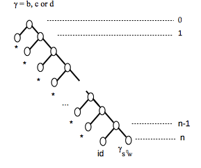
Figure 7.1. The letter $\gamma$ is in $\{b,c,d\}$ such that $\omega_{n-1}(\gamma)=id$. The symbol $\ast$ means the section is either $a$ or $id$.

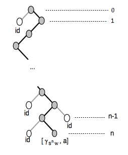
Figure 7.2. The element $\left[\gamma_{\mathfrak{s}^{n}\omega},a\right]$ is in the level $n$ rigid stabilizer. By definition, the element $\iota\left(\left[\gamma_{\mathfrak{s}^{n}\omega},a\right],v\right)$ only has nontrivial section at $v$.

Fact 7.6.

For $n\in\mathbb{N}$, let $\gamma$ be the letter in $\{b,c,d\}$ be such that $\omega_{n-1}(\gamma)=id$. Then for any vertex $v\in\mathsf{L}_{n}$, $\left[\gamma{}_{\mathfrak{s}^{n}\omega},a\right]$ is in the rigid stabilizer ${\rm Rist}_{G_{\omega}}(v)$ and

$$\left|\iota\left(\left[\gamma_{\mathfrak{s}^{n}\omega},a\right],v\right)\right|\leq 2^{n+2}.$$

Proof.

For each $n\in\mathbb{N}$, let $\gamma_{n}\in\{b,c,d\}$ be the letter that $\omega_{n-1}(\gamma_{n})=id$.

For each $n\geq 2$, fix a choice of letter $y_{n-1}\in\{b,c,d\}$ satisfying such that $\omega_{n-2}(y_{n-1})=id$ (that is, $y_{n-1}=\gamma_{n-1}$) if $\omega_{n-2}\neq\omega_{n-1}$; and $\omega_{n-2}(y_{n-1})=a$ if $\omega_{n-2}=\omega_{n-1}$. For $n=1$, fix a choice of letter $y_{0}$ such that $\omega_{0}(y_{0})=a$. Consider the Lysionok type substitution $\sigma_{n}$ on $\{a,b,c,d\}^{\ast}$ given by

$$a\mapsto ay_{n-1}a,\ b\mapsto b,\ c\mapsto c,\ d\mapsto d.$$

By definition of the substitution $\sigma_{n}$, we have that in one step wreath recursion, $\sigma_{n}\left(\left[a,\gamma_{n}\right]\right)=\left(id,\left[a,\gamma_{n}\right]\right)$.

Recall that $\mathbf{F}$ is the free product $\left(\mathbb{Z}/2\mathbb{Z}\right)\ast\left(\mathbb{Z}/2\mathbb{Z\times\mathbb{Z}}/2\mathbb{Z}\right)=\left\langle a\right\rangle\ast\left(\left\langle b\right\rangle\times\left\langle c\right\rangle\right)$. Denote by $K_{n}$ the normal closure of $[a,\gamma_{n}]$ in $\mathbf{F}$ and write $g^{h}$ for the conjugation $h^{-1}gh$. By direct calculation, in the first case where $\omega_{n-2}\neq\omega_{n-1}$, we have $y_{n-1}=\gamma_{n-1}$ and $\sigma_{n}\left([a,\gamma_{n}]\right)=a\gamma_{n-1}a\gamma_{n}a\gamma_{n-1}a\gamma_{n}=[a,\gamma_{n-1}][\gamma_{n-1},a]^{\gamma_{n}}$; while in the second case where $\omega_{n-2}=\omega_{n-1}$, we have $\gamma_{n-1}=\gamma_{n}$ and $\sigma_{n}\left([a,\gamma_{n}]\right)=ay_{n-1}a\gamma_{n}ay_{n-1}a\gamma_{n}=\left[a,\gamma_{n}\right]^{y_{n-1}a}[a,\gamma_{n}]$. It follows that for a word ${\bf w}\in K_{n}$, the image $\sigma_{n}({\bf w})$ is in $K_{n-1}$ and moreover, in one step wreath recursion, we have $\sigma_{n}\left({\bf w}\right)=\left(id,{\bf w}\right)$.

Let $v=v_{1}v_{2}\ldots v_{n}$ be the address of $v$. Apply the substitutions recursively: start with ${\bf w}_{0}=\gamma_{n}a\gamma_{n}a$, where $\gamma_{n}$ is the letter in $\{b,c,d\}$ be such that $\omega_{n-1}(\gamma_{n})=id$ as in the statement. For $0\leq j\leq n-1$, set

$${\bf w}_{j+1}=\begin{cases}\sigma_{n-j}({\bf w}_{j})&\mbox{if }v_{n-j}=1,\\ a\sigma_{n-j}({\bf w}_{j})a&\mbox{if }v_{n-j}=0.\end{cases}$$

It is understood that reduction in $\mathbf{F}$, for instance $a^{2}=1$, is always performed to words. For example $a(abac)^{2}a=\left(baca\right)^{2}$. Then it is clear that $|w_{j}|=2^{2+j}$.

We now verify that the word ${\bf w}_{n}$ obtained by substitutions as above evaluates to the desired element $\iota\left(\left[\gamma_{\mathfrak{s}^{n}\omega},a\right],v\right)$ in the group $G_{\omega}$. We start with ${\bf w}_{0}=[\gamma_{n},a]\in K_{n}$. Then by the property of the substitutions above, for $0\leq j\leq n-1$, under one step wreath recursion we have

$${\bf w}_{j+1}=\begin{cases}(id,{\bf w}_{j})&\mbox{if }v_{n-j}=1,\\ ({\bf w}_{j},id)&\mbox{if }v_{n-j}=0.\end{cases}$$

Therefore perform the recursion to ${\bf w}_{n}$ down $n$ levels, we have that under the projection $\pi_{\omega}:\mathbf{F}\to G_{\omega}$ given by $a\mapsto a$, $b\mapsto b_{\omega}$, $c\mapsto c_{\omega}$ and $d\mapsto d_{\omega}$, it evaluates to $\iota\left(\left[\left(\gamma_{n}\right)_{\mathfrak{s}^{n}\omega},a\right],v\right)$.

∎

For $k,n\in\mathbb{N}$ both divisible by $D$, define the set $\mathsf{W}_{k}^{n}$ of vertices of depth $k$ such that $u_{i}=1$ except for those $i$ with $n+i\in I_{\omega}$,

(7.2) $$\mathsf{W}_{k}^{n}:=\left\{u\in\mathsf{L}_{k}:\ u=u_{1}\ldots u_{k},\ u_{i}=1\mbox{ if }n+i\notin I_{\omega}\right\}.$$

Recall that the set $I_{\omega}$ is defined in Notation 7.1. The cardinality of the set $\mathsf{W}_{k}^{n}$ is $2^{k/D}$.

Given an integer $j$, denote by $\bar{j}$ the residue of $j$ mod $D$, $\bar{j}\in\{0,\ldots,D-1\}$. We now define the set $\mathsf{V}_{k}^{j}$ which will be the index set of a collection of conjugates of the element $c_{s^{j}\omega}$ in $G_{j}=G_{\mathfrak{s}^{j}\omega}$. Let $k$ be an integer divisible by $D$, write $\ell(k,j)=\frac{1}{D}\left(j+D-\bar{j}+k\right)$ and define $\mathsf{V}_{k}^{j}$ the collection of vertices

(7.3) $$\mathsf{V}_{k}^{j}:=\left\{1^{D-\bar{j}}u1^{m_{\ell(j,k)}+2}0:\ u\in\mathsf{W}_{k}^{j+D-\bar{j}}\right\},$$

where $m_{\ell}$ is defined in Notation 7.1, $m_{\ell}\in\{0,\ldots,D-3\}$. In words, $\mathsf{V}_{k}^{j}$ is obtained from the set $\mathsf{W}_{k}^{j+D-\bar{j}}$ by appending some $1$’s as prefix to match with $D$-blocks and adding $1^{m_{\ell(j,k)}+2}0$ at the end. It is important that any $v\in\mathsf{V}_{k}^{j}$ ends with digit $0$. The cardinality of the set $V_{k}^{j}$ is $2^{k/D}$, the same as the cardinality of $\mathsf{W}_{k}^{j+D-\bar{j}}$.

Given a vertex $v=v_{1}\ldots v_{k^{\prime}}\in\mathsf{V}_{k}^{j}$, where $k^{\prime}=D-\bar{j}+k+m_{\ell(j,k)}+3$ denotes the length of $v$, take the following sequence of elements in $G_{j}=G_{\mathfrak{s}^{j}\omega}$:

(7.4) $$h_{i}^{v}:=\begin{cases}id&\mbox{if }v_{i}=1\\ \iota\left(\left[b_{\mathfrak{s}^{j+i-2}\omega},a\right],v_{1}\ldots v_{i-2}\right)&\mbox{if }v_{i}=0.\end{cases}$$

By definition of $\mathsf{V}_{k}^{j}$ in (7.3), if $v_{i}=0$ then the string $\omega_{j+i-3}\omega_{j+i-2}\omega_{j+i-1}$ is either ${\bf 201}$ or ${\bf 211}$. Since the digit $\omega_{j+i-3}$ in this case must be ${\bf 2}$, by Fact 7.6, $\left[b_{\mathfrak{s}^{j+i-2}\omega},a\right]$ is in the rigid stabilizer of the vertex $v_{1}\ldots v_{i-2}$ in $G_{j}$. The letter following $\omega_{j+i-3}$ is different from ${\bf 2}$, therefore $\left[b_{\mathfrak{s}^{j+i-2}\omega},a\right]$ acts as $b_{\mathfrak{s}^{j+i-1}\omega}a$ on the right subtree. Since $h_{i}^{v}$ is in the rigid stabilizer of $v_{1}\ldots v_{i-2}$, it is easy to verify recursively that by definition of the elements $h_{i}^{v}$ in (7.4), we have

$$1^{\infty}\cdot h_{1}^{v}h_{2}^{v}\ldots h_{k^{\prime}}^{v}=v1^{\infty}.$$

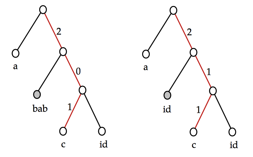
Figure 7.3. A conjugated element for $v=110$, the only label $c$ is at $v$ (the corresponding ray is red). The picture shows a turn over $\bf{201}$ on the left and a turn over $\bf{211}$ on the right, in general notation.

For each $v\in\mathsf{V}_{k}^{j}$, take the conjugation of $c_{\mathfrak{s}^{j}\omega}$ in $G_{j}$

(7.5) $$\mathfrak{c}_{j}^{v}:=\left(h_{1}^{v}h_{2}^{v}\ldots h_{k^{\prime}}^{v}\right)^{-1}c_{\mathfrak{s}^{j}\omega}\left(h_{1}^{v}h_{2}^{v}\ldots h_{k^{\prime}}^{v}\right).$$

We have the following description of the element $\mathfrak{c}_{j}^{v}$. The portrait of an element along a ray segment is explained in Subsection 2.5.

Lemma 7.7.

Let $v\in\mathsf{V}_{k}^{j}$, $D|k$ and write $k^{\prime}=|v|$ the length of $v$. The vertex $v$ is fixed by $\mathfrak{c}_{j}^{v}$ and along the ray segment $v$ the only nontrivial sections of $\mathfrak{c}_{j}^{v}$ are at

$$\{v_{1}\ldots v_{i}0:\ \omega_{j+i}\neq{\bf 1},\ 0\leq i\leq k^{\prime}-1\}.$$

Among these, for $i\leq k^{\prime}-2$ and $\omega_{j+i}\neq{\bf 1}$, if $v_{i+2}=0$ then the section at $v_{1}\ldots v_{i}0$ is $b_{\mathfrak{s}^{j+i+1}\omega}ab_{\mathfrak{s}^{j+i+1}\omega}$, otherwise the section is $a$. For $i=k^{\prime}-1$, at level $k^{\prime}$, the only non-trivial section is $c_{\mathfrak{s}^{j+k^{\prime}}\omega}$ at $v$.

Proof.

For those indices $i$ such that $v_{i}=0$, conjugation by $h_{i}^{v}$ is nontrivial only in the subtree rooted at $v_{1}\ldots v_{i-2}$, where the section is conjugated by $\left[b_{\mathfrak{s}^{j+i-2}\omega},a\right]$. Effect of conjugation by $\left[b_{\mathfrak{s}^{j+i-2}\omega},a\right]$ is drawn explicitly in Figure 7.3 with subscripts omitted. The portrait of $\mathfrak{c}_{j}^{v}$ is obtained by applying these conjugations one by one (where every non-trivial conjugation corresponding to a $0$ in $v$ results in a turn illustrated in the pictures).

∎

Remark 7.8.

The reason we need ${\bf 201}$ or ${\bf 211}$ in Assumption $({\rm Fr}(D))$ to perform these conjugations is the following: the digit ${\bf 2}$ is needed for $[b,a]$ to be in the rigid stabilizer at the corresponding level, the second digit different from ${\bf 2}$ implies $[b,a]$ acts as $ab,ba$ on the next level, and the last digit ${\bf 1}$ implies that the sections of $c$ that gets swapped are $c$ and $id$. As a consequence, $\mathfrak{c}_{j}^{v}$ fixes the ray $1^{\infty}$ and vertices of the form $1^{m}0$. It is possible that the arguments can work through under the weaker assumption that one can find ${\bf 20}$ or ${\bf 21}$ in every $D$-block, but it simplifies calculations to assume the third digit is ${\bf 1}$.

Figure 7.4. Portrait of the element $\tilde{g}_{j}^{v}$ with $j=3$ and $v=11(111)(110)(110)(110)$ in the first Grigorchuk group, with usual notation. Because of space limitations the picture does not show the full portrait: in places marked as … there are two types of portraits: the portrait in the subtree at a black vertex is the same as at $000$; and in the subtree at a white vertex, the portrait is the same as at $100$.

Next we apply the substitutions $\zeta_{x}$ to $a\mathfrak{c}_{j}^{v}$, which is an element in $G_{j}$, to obtain an element in $G_{\omega}$. Given $j$ and a vertex $v\in\mathsf{V}_{k}^{j}$ where $D|k$, define

(7.6) $$\tilde{g}_{j}^{v}:=\zeta_{\omega_{0}}\circ\ldots\circ\zeta_{\omega_{j-1}}\left(a\mathfrak{c}_{j}^{v}\right).$$

Figure 7.4 illustrates the portrait of an element of this type in the first Grigorchuk group. element $\tilde{g}_{j}^{v}$, with $j=3$ and $v=11111110110110$, in the first Grigorchuk group $G_{012}$.

Lemma 7.9.

The element $\tilde{g}_{j}^{v}$ is well defined (the substitutions $\zeta_{\omega_{i}}$’s can be applied). It is in the $j$-th level stabilizer and when $\omega_{j-1}\neq{\bf 1}$, the sections of $\tilde{g}_{j}^{v}$ at vertices of $\mathsf{L}_{j}$ are in $\left\{a\mathfrak{c}_{j}^{v},\mathfrak{c}_{j}^{v}a\right\}$ .

Proof.

In $G_{j}$, each non-trivial $h_{i}^{v}$ is defined to be $\iota\left(\left[b_{\mathfrak{s}^{j+i-2}\omega},a\right],v_{1}\ldots v_{i-2}\right)$. As explained in the proof of Fact 7.6, the element $h_{i}^{v}$ can be represented as a reduced word in $\left\{ab,ac,ad\right\}^{\ast}$, under the projection $\pi_{\mathfrak{s}^{j}\omega}:\mathbf{F}\to G_{\mathfrak{s}^{j}\omega}$. It follows that after applying the conjugations to $c$, the element $\mathfrak{c}_{j}^{v}$ can be represented either by a reduced word of the form $wa$, where $w\in\{ab,ac,ad\}^{\ast}$, or by $\gamma w$ where $\gamma\in\{b,c,d\}$ and $w\in\{ab,ac,ad\}^{\ast}$. In first case $a\mathfrak{c}_{j}^{v}$ can be represented by a word in $\{ba,ca,da\}^{\ast}$, in the second case it can be represented by a word in $\{ab,ac,ad\}^{\ast}$. In either case the substitutions $\zeta_{\omega_{i}}$ can be applied to $a\mathfrak{c}_{j}^{v}$. The second claim follows from (2.3).

∎

We now summarize what we have defined so far. For any integer $j$ (indicating the level) and integer $k$ divisible by $D$ (parametrizing the length of the segment where conjugations are performed), we have defined an index set $V_{k}^{j}$ as in (7.3). For each string $v\in V_{k}^{j}$, we take the conjugated element $\mathfrak{c}_{j}^{v}$ in $G_{\mathfrak{s}^{j}\omega}$ as defined in (7.5) and use the substitutions $\zeta_{x}$ to obtain an element $\tilde{g}_{j}^{v}$ in $G_{\omega}$ as defined in (7.6). Keep in mind the picture that the portrait of $\mathfrak{c}_{j}^{v}$ is directed along $v$, see Figure 1.3 and at each vertex in $\mathsf{L}_{j}$, the section of $\tilde{g}_{j}^{v}$ is either $a\mathfrak{c}_{j}^{v}$ or $\mathfrak{c}_{j}^{v}a$, see Figure 7.4.

Let $(k_{n})$ be a sequence of increasing positive integers divisible by $D$ to be determined later, $k_{n}\ll n$. In what follows $n$ is always an integer divisible by $D$. For each $j\in\{1,\ldots,n\}$, take the following sets $\mathfrak{F}_{j,n}$ of group elements in $G_{\omega}$,

• For an index $j$ such that $\omega_{j-1}={\bf 2}$ and $n-k_{n}<j\leq n$, define $\mathfrak{F}_{j,n}$ to be the following set of elements $\tilde{g}_{j}^{v}=\zeta_{\omega_{0}}\circ\ldots\circ\zeta_{\omega_{j-1}}\left(a\mathfrak{c}_{j}^{v}\right)$,

  (7.7) $$\mathfrak{F}_{j,n}:=\left\{\tilde{g}_{j}^{v}|\ v\in\mathsf{V}_{2k_{n}}^{j}\mbox{ and }\left|1^{\infty}\wedge v\right|\geq n-j+D\right\},$$

  where $u\wedge v$ denotes the longest common prefix of two rays $u$ and $v$. The set $\mathfrak{F}_{j,n}$ is indexed by the subset of $\mathsf{V}_{2k_{n}}^{j}$ which consists of vertices with prefix $1^{n-j+D}$. The cardinality of $\mathfrak{F}_{j,n}$ is $2^{\frac{2k_{n}-(n-j+\bar{j})}{D}}$ in this case.

• Otherwise, that is, for indices $j\in\{1,\ldots,n\}$ other than those with $\omega_{j-1}={\bf 2}\mbox{ and }n-k_{n}<j\leq n$, keep the single element $g_{j}$ and set $\mathfrak{F}_{j,n}=\{g_{j}\}$, where $g_{j}$ is defined in (7.1).

Informally, for those indices $j$ within $k_{n}$ distance to $n$ with "bad" germs, we replace $g_{j}$ by a set $\mathfrak{F}_{j,n}$ of conjugated elements parametrized by strings; while for those $g_{j}$’s with "good" germs, we keep them as they are.

We proceed to construct a measure $\upsilon_{n}$ on $G_{\omega}$ which will replace the $n$-quasi-cubic measure. A random element with distribution $\upsilon_{n}$ can be obtained as follows. Take independent random variables $\{\epsilon_{i},\gamma_{i}|\ 1\leq i\leq n\}$ where for each $i$, $\epsilon_{i}$ is uniform on $\{0,1\}$ and $\gamma_{i}$ is uniform on the set $\mathfrak{F}_{i,n}$. Then the group element $\gamma_{n}^{\epsilon_{n}}\ldots\gamma_{1}^{\epsilon_{1}}$ has distribution $\upsilon_{n}$. We refer to $\upsilon_{n}$ as a uniformised $n$-quasi-cubic measure, it depends on the parameters $(k_{n})$. The measure $\upsilon_{n}$ is similar to an $n$-quasi-cubic measure considered in earlier sections, but with an extra layer of randomness in the choice of the cube independent sequence $\gamma_{1},\ldots\gamma_{n}$.

More formally, the distribution $\upsilon_{n}$ is defined as follows. Take the direct product

(7.8) $$\mathfrak{F}_{n}=\prod_{i=1}^{n}\mathfrak{F}_{i,n}$$

and the product of the hypercube $\{0,1\}^{n}$ with $\mathfrak{F}_{n}$,

(7.9) $$\varLambda_{n}=\{0,1\}^{n}\times\mathfrak{F}_{n}.$$

Define $\theta_{n}:\varLambda_{n}\to G_{\omega}$ to be the map

$$\theta_{n}\left(\left(\boldsymbol{\epsilon},\boldsymbol{\gamma}\right)\right)=\gamma_{n}^{\epsilon_{n}}\ldots\gamma_{1}^{\epsilon_{1}},$$

where $\boldsymbol{\epsilon}=\left(\epsilon_{1},\ldots,\epsilon_{n}\right)\in\{0,1\}^{n}$ and $\boldsymbol{\gamma}=\left(\gamma_{1},\ldots,\gamma_{n}\right)$, $\gamma_{i}\in\mathfrak{F}_{i,n}$. Take the measure $\upsilon_{n}$ on $G_{\omega}$ to be the push-forward of the uniform measure $\mathbf{u}_{\varLambda_{n}}$ under $\theta_{n}$, that is

(7.10) $$\upsilon_{n}(g)=\frac{\left|\{\left(\boldsymbol{\epsilon},\boldsymbol{\gamma}\right)\in\varLambda_{n}:\theta_{n}\left(\left(\boldsymbol{\epsilon},\boldsymbol{\gamma}\right)\right)=g\}\right|}{|\varLambda_{n}|}.$$

For the purpose of symmetrization, set the measure $\check{\upsilon}_{n}$ to be

$$\check{\upsilon}_{n}(g)=\upsilon_{n}\left(g^{-1}\right).$$

Finally, for $\beta\in(0,1)$, take the convex combination of the measures

(7.11) $$\mu_{\beta}=\frac{1}{2}\mathbf{u}_{S}+\frac{1}{2}\sum_{n\in\mathbb{N},D|n}C_{\beta}2^{-n\beta}\left(\upsilon_{n}+\check{\upsilon}_{n}\right),$$

where ${\bf u}_{S}$ is the uniform measure on the generating set $\{a,b_{\omega},c_{\omega},d_{\omega}\}$, $C_{\beta}>0$ is the normalization constant such that $\mu_{\beta}$ is a probability measure. Note that although suppressed in the notations, the measure $\mu_{\beta}$ depends on the sequence $(k_{n})$.

Example 7.10.

We explain the definitions on the first Grigorchuk group $G=G_{{\bf 012}}$, in the usual notation as in (2.4). The correspondence between two systems of notations (usual and general) on $G$ is explained in (2.5).

The defining string of $G$ is $({\bf 012})^{\infty}={\bf 01}({\bf 201})^{\infty}$, with a shift of two digits it satisfies Assumption ${\rm Fr}(D)$, $D=3$. In Notation 7.1, for the shifted string $\omega=({\bf 201})^{\infty}$, we have $m_{k}=0$ and $I_{\omega}=3\mathbb{N}$.

On $G$ the sequence $(g_{n})$ defined in formula (7.1) is

$$g_{j}=\begin{cases}\zeta^{j}(ac)&\mbox{if }j\equiv 0,1\mod 3,\\ \zeta^{j}(ad)&\mbox{if }j\equiv 2\mod 3,\end{cases}$$

in the usual notation for the first Grigorchuk group. This sequence has appeared in Subsection 5.2 and Section 6. Among them those $g_{j}$ with $j\equiv 0\mod 3$ have $c$-germs, for which we will perform the conjugations.

In what follows $k$ is divisible by $3$ and $n\equiv 2\mod 3$ (where $2$ comes from the shift of two digits from $({\bf 012})^{\infty}$ to $({\bf 201})^{\infty}$). The set $\mathsf{W}_{k}^{n}$ defined in (7.2) is

$$\mathsf{W}_{k}^{n}=\left\{u:\ |u|=k\mbox{ and }u_{3j+1}=u_{3j+2}=1\mbox{ for all }j\geq 0\right\}.$$

In other words, $\mathsf{W}_{k}^{n}$ consists of vertices of length $k$ that are concatenations of segments $111$ and $110$. For $j\equiv 0\mod 3$, the set $\mathsf{V}_{k}^{j}$ defined in (7.3) is

$$\mathsf{V}_{k}^{j}=\left\{11u110:\ u\in\mathsf{W}_{k}^{j+2}\right\},$$

that is vertices of the form $11\underbrace{(11\ast)\ldots(11\ast)}_{k\ {\rm digits}}110$, where at $\ast$ the digit can be $0$ or $1$. The cardinality of the set $\mathsf{V}_{k}^{j}$ is $2^{k/3}$.

We remark that the set $\mathsf{V}_{k}^{j}$ is contained in the ${\rm H}^{b}$-orbit of the vertex $1^{2+k+3}$, where ${\rm H}^{b}$ is the subgroup of $G$ which consists of elements with only $\left\langle b\right\rangle$-germs, see Figure 7.5.

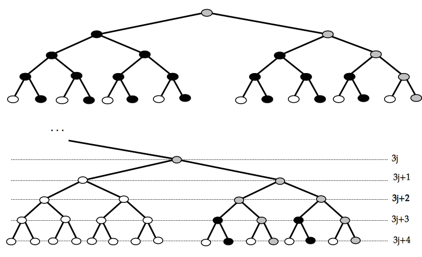
Figure 7.5. Colors grey and black mark vertices that are in the orbit of the rightmost ray under $\rm{H}^{b}$. These are vertices of the form $(\ast)(\ast\ast 1)(\ast\ast 1)\dots$. The subsets of grey vertices on levels $\equiv 2\mod 3$ show vertices that are in the indexing set for conjugaction in the definition of $\mathfrak{c}^{v}$. They are of the form $(11)(11\ast)(11\ast)\dots$.

Figure 1.4 draws the portrait of a conjugated element $\mathfrak{c}^{v}=\mathfrak{c}_{j}^{v}$ indexed by $v\in\mathsf{V}_{k}^{j}$ as defined in (7.5). Note that since $({\bf 012})^{\infty}$ is of period $3$, for all $j\equiv 0\mod 3$, $\mathfrak{c}_{j}^{v}$ is the same element, thus we can omit reference to $j$.

For $n\equiv 2\mod 3$, take a parameter $k_{n}$ divisible by $3$. In the sequence $(g_{j})_{j=1}^{n}$, for these $j\leq n-k_{n}$ or $j\equiv 1,2\mod 3$, let $\mathfrak{F}_{j,n}=\{g_{j}\}$; for these $j$ such that $j\equiv 0\mod 3$ and $n-k_{n}<j\leq n$, replace $g_{j}$ by the set $\mathfrak{F}_{j,n}$ defined in (7.7), which is

$$\mathfrak{F}_{j,n}=\left\{\zeta^{j}(a\mathfrak{c}_{j}^{v}):\ v=11\underbrace{(11\ast)\ldots(11\ast)}_{2k_{n}\ {\rm digits}}110\mbox{ and }v\mbox{ has prefix }1^{n-j+3}\right\}.$$

The uniformised $n$-quasi-cubic measure $\upsilon_{n}$ can be described as follows. For $1\leq j\leq n$, independently choose each $\gamma_{j}$ uniformly from the set $\mathfrak{F}_{j,n}$, and choose an independent random variable $(\epsilon_{1},\ldots,\epsilon_{n})$ uniformly from $\{0,1\}^{n}$, then the random group element $\gamma_{n}^{\epsilon_{n}}\ldots\gamma_{1}^{\epsilon_{n}}$ has distribution $\upsilon_{n}$.

Finally the measure $\mu_{\beta}$ defined with parameter sequence $(k_{n})$ in (7.11) is a convex combination of ${\bf u}_{S}$, $S=\{a,b,c,d\}$ and the uniformised $n$-quasi-cubic measures $\upsilon_{n}$ and their inverses $\check{\upsilon}_{n}$, over all $n\equiv 2\mod 3$.

7.3. Non-triviality of the Poisson boundary

The goal of this subsection is to show that with some appropriate choices of $\beta$ and $A$, the measure $\mu_{\beta}$ defined in (7.11) with $k_{n}=A\left\lfloor\log_{2}n\right\rfloor$ has non-trivial Poisson boundary.

Recall that as explained in Example 3.2, the isotropy group of the groupoid of germs of $G_{\omega}\curvearrowright\partial\mathsf{T}$ at $1^{\infty}$ is isomorphic to $\mathbb{Z}/2\mathbb{Z}\times\mathbb{Z}/2\mathbb{Z}=\left\langle b\right\rangle\times\left\langle c\right\rangle$. An element $g\in G_{\omega}$ has only $\left\langle b\right\rangle$-germs if and only if there is a level $n$ such that all sections $g_{v}$ are in $\left\{id,a,b_{\mathfrak{s}^{n}\omega}\right\}$, $v\in\mathsf{L}_{n}$. Let $H=\left\langle b\right\rangle<\left(\mathcal{G}_{\omega}\right)_{o}$ and $\mathcal{H}^{b}$ be the set of germs that are either trivial or $b$ as in (3.1). To apply Proposition 3.3, we need to verify that the summation

$$\sum_{x\in o\cdot G}{\bf G}_{P_{\mu_{\beta}}}(o,x)\mu_{\beta}\left(\left\{g\in G:\ (g,x)\notin\mathcal{H}^{b}\right\}\right)$$

is finite, where $P_{\mu_{\beta}}$ is the transition kernel induced by $\mu_{\beta}$ on the orbit $o\cdot G$. To this end we show separately an upper estimate on the Green function and a bound on the $\mu_{\beta}$-weights in the summation.

Proposition 7.11.

Let $\beta\in(1-\frac{1}{D},1)$ and $k_{n}=A\left\lfloor\log_{2}n\right\rfloor$. For any $\epsilon>0$, there exists a constant $C=C(\beta,D,\epsilon)>0$ such that for any $x,y\in 1^{\infty}\cdot G$, the Green function satisfies

$$\mathbf{G}_{P_{\mu_{\beta}}}(x,y)\leq C\left(\frac{d_{\mathcal{S}}(x,y)}{\log_{2}^{2A}d_{\mathcal{S}}(x,y)}\right)^{\beta-1}(\log_{2}d_{\mathcal{S}}(x,y))^{-\frac{1-\beta}{1+\beta}\left(\frac{2A}{D}-\epsilon\right)}.$$

Proposition 7.11 is proved in Subsection 7.5, it is a consequence of the off-diagonal upper bound for transition probabilities in [BGK]. For the $\mu_{\beta}$-weights in the summation, we have the following.

Proposition 7.12.

Let $\upsilon_{n}$ be defined as in (7.10) and $o=1^{\infty}$. Let $f:\mathbb{R}_{+}\to\mathbb{R}_{+}$ be a non-increasing function such that there exists constants $D^{\prime}\in(D,\infty)$,

$$\frac{f\left(2x\right)}{f(x)}\geq 2^{-\frac{1}{D^{\prime}}}\mbox{ for all }x\geq 1.$$

Then there exists a constant $C=C(D^{\prime})<\infty$ such that

$$\sum_{x\in o\cdot G}f\left(d_{\mathcal{S}}(o,x)\right)\upsilon_{n}\left(\left\{g\in G:\ (g,x)\notin\mathcal{H}^{b}\right\}\right)\leq C2^{n}f\left(2^{n+2k_{n}}\right).$$

The same inequality holds with $\upsilon_{n}$ replaced by $\check{\upsilon}_{n}$.

Proposition 7.12 is proved in Subsection 7.6. With these two estimates we prove that for some appropriate choice of parameters, along the random walk trajectory the $\left\langle b\right\rangle$-coset of the germ at $1^{\infty}$ stabilizes.

Theorem 7.13.

Let $\omega$ be a string satisfying Assumption $({\rm Fr}(D))$. Then for $\beta\in\left(1-\frac{1}{D},1\right)$ and integer $A>\frac{D(1+\beta)}{2(1-\beta)}$ divisible by $D$, the measure $\mu_{\beta}$ on $G_{\omega}$ defined as in (7.11) with $k_{n}=A\left\lfloor\log_{2}n\right\rfloor$ has non-trivial Poisson boundary.

Proof of Theorem 7.13 given Prop. 7.11 and 7.12.

We show that the summation

$$\sum_{x\in o\cdot G}{\bf G}_{P_{\mu_{\beta}}}(o,x)\mu_{\beta}\left(\left\{g\in G:\ (g,x)\notin\mathcal{H}^{b}\right\}\right)$$

is finite, then non-triviality of the Poisson boundary $\left(G_{\omega},\mu_{\beta}\right)$ follows from Proposition 3.3.

Let $\epsilon>0$ be a small constant such that $\frac{1-\beta}{1+\beta}\left(\frac{2A}{D}-\epsilon\right)>1$. By Proposition 7.11, there is a constant $C<\infty$ only depending on $\beta,D,\epsilon$ such that

$$\mathbf{G}_{P_{\mu_{\beta}}}(x,y)\leq C\left(\frac{d_{\mathcal{S}}(x,y)}{\log_{2}^{2A}d_{\mathcal{S}}(x,y)}\right)^{\beta-1}(\log_{2}d_{\mathcal{S}}(x,y))^{-\frac{1-\beta}{1+\beta}\left(\frac{2A}{D}-\epsilon\right)}.$$

Let $f(s)=C\left(\frac{s}{\log_{2}^{2A}s}\right)^{\beta-1}\left(\log_{2}s\right)^{-\frac{1-\beta}{1+\beta}\left(\frac{2A}{D}-\epsilon\right)}.$ Then $f$ satisfies the assumption of Proposition 7.12 with $D^{\prime}=\frac{1}{1-\beta}>D$. By Proposition 7.12,

$$\sum_{x\in o\cdot G}{\bf G}_{P_{\mu_{\beta}}}(o,x)\frac{\upsilon_{n}+\check{\upsilon}_{n}}{2}\left(\left\{g\in G:\ (g,x)\notin\mathcal{H}^{b}\right\}\right)$$

$$\leq \sum_{x\in o\cdot G}f(d_{\mathcal{S}}(o,x))\frac{\upsilon_{n}+\check{\upsilon}_{n}}{2}\left(\left\{g\in G:\ (g,x)\notin\mathcal{H}^{b}\right\}\right)$$

$$\leq C^{\prime}2^{n}f\left(2^{n+2k_{n}}\right),$$

where $C^{\prime}$ is a constant depending only on $\beta$. Summing up this estimate to $\mu_{\beta}$,

$$\sum_{x\in o\cdot G}{\bf G}_{P_{\mu_{\beta}}}(o,x)\mu_{\beta}\left(\left\{g\in G:\ (g,x)\notin\mathcal{H}^{b}\right\}\right)$$

$$\leq C_{\beta}\sum_{D|n}\sum_{x\in o\cdot G}f(d_{\mathcal{S}}(o,x))2^{-n\beta}\frac{\upsilon_{n}+\check{\upsilon}_{n}}{2}\left(\left\{g\in G:\ (g,x)\notin\mathcal{H}^{b}\right\}\right)$$

$$\leq C_{\beta}C^{\prime}\sum_{D|n}2^{-n\beta}2^{n}f\left(2^{n+2k_{n}}\right)$$

$$\leq C_{\beta}C^{\prime}C\sum_{D|n}2^{n(1-\beta)}\left(\frac{2^{n+2k_{n}}}{(n+2k_{n})^{2A}}\right)^{\beta-1}\left(n+2k_{n}\right)^{-\frac{1-\beta}{1+\beta}\left(\frac{2A}{D}-\epsilon\right)}$$

$$\leq C_{\beta}C^{\prime}C\sum_{n=1}^{\infty}n^{-\frac{1-\beta}{1+\beta}\left(\frac{2A}{D}-\epsilon\right)}.$$

In the last step we plugged in $k_{n}=A\left\lfloor\log_{2}n\right\rfloor$. Since the constant $A$ is assumed to satisfy $\frac{1-\beta}{1+\beta}\left(\frac{2A}{D}-\epsilon\right)>1$, it follows that the summation is finite.

∎

The rest of the section is devoted to the proofs of Proposition 7.11 (in Subsection 7.5) and Proposition 7.12 (in Subsection 7.6), with some preparation given in Subsection 7.4.

7.4. Estimates on the induced transition kernel

In this subsection we give some bounds on the transition kernel $P_{\mu_{\beta}}$, which will be used to derive Green function upper bounds. We use definitions and notations from Subsection 7.2.

By the definition of the set $\mathfrak{F}_{j,n}$ in (7.7) we have the following:

Fact 7.14.

Let $j$ be an index such that $\omega_{j-1}={\bf 2}$ and $n-k_{n}<j\leq n$. Then on the finite level $n+D+1$, the action of any element $\tilde{g}_{j}^{v}\in\mathfrak{F}_{j,n}$ is the same as the element $g_{j}$.

Proof.

This is because in the definition of $\mathfrak{F}_{j,n}$, the ray segment $v$ is required to satisfy $|v\wedge 1^{\infty}|\geq n-(j-\bar{j})+D$. The first level that sees the difference between the portraits of $\tilde{g}_{j}^{v}$ and $g_{j}$ is $\geq n+D+2$.

∎

Because of the previous fact, the following uniqueness property is inherited from $(g_{n})$.

Lemma 7.15.

Let $x\in\mathsf{L}_{n+D+1}$. Suppose $\left(\epsilon_{i},\gamma_{i}\right)_{i=1}^{n},\left(\tilde{\epsilon}_{i},\tilde{\gamma}_{i}\right)_{i=1}^{n}\in\varLambda_{n}$ are such that

$$x\cdot\gamma_{n}^{\epsilon_{n}}\ldots\gamma_{1}^{\epsilon_{1}}=x\cdot\tilde{\gamma}_{n}^{\tilde{\epsilon}_{n}}\ldots\tilde{\gamma}_{1}^{\tilde{\epsilon}_{1}}.$$

Then $\epsilon_{i}=\tilde{\epsilon}_{i}$ for all $1\leq i\leq n$.

We derive a displacement estimate from Lemma 7.5 and description of elements in $\mathfrak{F}_{j,n}$ from Lemma 7.7 and Lemma 7.9.

Lemma 7.16.

Let $j$ be an index such that $\omega_{j-1}={\bf 2}$ and $n-k_{n}<j\leq n$. Let $\tilde{g}_{j}^{v}\in\mathfrak{F}_{j,n}$, then for any $x\in 1^{\infty}\cdot G$,

$$d_{\mathcal{S}}\left(x,x\cdot\tilde{g}_{j}^{v}\right)\leq\begin{cases}2^{j+|\mathfrak{s}^{j+1}x\wedge\mathfrak{s}v|+4}&\mbox{if }|\mathfrak{s}^{j+1}x\wedge\mathfrak{s}v|\geq n-j+D,\\ 2^{j+2}&\mbox{if }|\mathfrak{s}^{j+1}x\wedge\mathfrak{s}v|<n-j+D.\end{cases}$$

Proof.

We show the second bound first. Since by definitions, $v$ has prefix $1^{n-j+\bar{j}+D}$, $|\mathfrak{s}^{j+1}x\wedge\mathfrak{s}v|<n-j+D$ implies that $|\mathfrak{s}^{j+1}x\wedge 1^{\infty}|<n-j+D$. In this case the action of $\tilde{g}_{j}^{v}$ on $x$ is the same as $g_{j}$, that is $x\cdot\tilde{g}_{j}^{v}=x\cdot g_{j}$. Therefore

$$d_{\mathcal{S}}\left(x,x\cdot\tilde{g}_{j}^{v}\right)=d_{\mathcal{S}}(x,x\cdot g_{j})\leq 2^{j+2}.$$

Now suppose $|\mathfrak{s}^{j+1}x\wedge\mathfrak{s}v|\geq n-j+D$. By definition of $\tilde{g}_{j}^{v}$ and Lemma 7.9, depending parity of $\sum_{i=1}^{j}x_{i}$, we need to consider $(\mathfrak{s}^{j}x)\cdot a\mathfrak{c}_{j}^{v}$ or $(\mathfrak{s}^{j}x)\cdot\mathfrak{c}_{j}^{v}a$. By description of $\mathfrak{c}_{j}^{v}$ in Lemma 7.7 and the distance bound in Lemma 7.5, we have that for any ray $y$,

$$d_{\mathcal{S}}(y,y\cdot\mathfrak{c}_{j}^{v})\leq 2^{|y\wedge v|+4}.$$

Since

$$d_{\mathcal{S}}\left(x,x\cdot\tilde{g}_{j}^{v}\right)\leq 2^{j}\max\left\{d_{\mathcal{S}}(\mathfrak{s}^{j}x,\left(\mathfrak{s}^{j}x\right)\cdot a\mathfrak{c}_{j}^{v}),d_{\mathcal{S}}(\mathfrak{s}^{j}x,\left(\mathfrak{s}^{j}x\right)\cdot\mathfrak{c}_{j}^{v}a)\right\},$$

the claim follows.

∎

Lemma 7.16 implies that

$$\max_{\gamma\in\mathfrak{F}_{j,n}}d_{S}(x,x\cdot\gamma)\leq 2^{j+2k_{n}+2D+4}.$$

By the triangle inequality, for any $x$ and $\boldsymbol{\epsilon}\in\{0,1\}^{n}$,

$$\max_{\boldsymbol{\gamma}\in\mathfrak{F}_{n}}d_{S}(x,x\cdot\gamma_{n}^{\epsilon_{n}}\ldots\gamma_{1}^{\epsilon_{1}})\leq 2^{n+2k_{n}+2D+5}.$$

The purpose of introducing the conjugations $\mathfrak{c}_{j}^{v}$ and randomizing over $v$ in the construction of the measure $\upsilon_{n}$ is to average so that the tail decays of measures is lighter than the maximum indicated above.

Lemma 7.17.

We have the following upper bounds:

(i):

Let $j$ be a level such that $n-k_{n}\leq j\leq n$ and $\omega_{j-1}={\bf 2}$. For any $\ell$ such that $n\leq\ell\leq j+2k_{n}+2D+4$ and $x\in 1^{\infty}\cdot G$,

$${\bf u}_{\mathfrak{F}_{j,n}}\left(\left\{\gamma:\ d_{\mathcal{S}}(x,x\cdot\gamma)\geq 2^{\ell}\right\}\right)\leq 2^{-\frac{1}{D}\left(\ell-n\right)+2}.$$

(ii):

For any $\left(\epsilon_{1},\ldots,\epsilon_{n}\right)\in\{0,1\}^{n}$, $n\leq\ell\leq n+2k_{n}+2D+5$ and $x\in 1^{\infty}\cdot G$,

$${\bf u}_{\mathfrak{F}_{n}}\left(\left\{\boldsymbol{\gamma}:\ d_{\mathcal{S}}\left(x,x\cdot\gamma_{n}^{\epsilon_{n}}\ldots\gamma_{1}^{\epsilon_{1}}\right)\geq k_{n}2^{\ell}\right\}\right)\leq 8k_{n}2^{-\frac{1}{D}(\ell-n)}.$$

Proof.

(i). By Lemma 7.16, for such $\ell$,

$${\bf u}_{\mathfrak{F}_{j,n}}\left(\left\{\gamma:\ d_{S}(x,x\cdot\gamma)\geq 2^{\ell}\right\}\right)\leq{\bf u}_{\mathfrak{F}_{j,n}}\left(\left\{\tilde{g}_{3j}^{v}:\ \left|\mathfrak{s}^{j+1}x\wedge\mathfrak{s}v\right|\geq\ell-j-4\right\}\right).$$

Recall that $\mathfrak{F}_{j,n}$ is indexed by strings $v\in\mathsf{V}_{2k_{n}}^{j}$ and $\left|1^{\infty}\wedge v\right|\geq n-j+D$. The number of such strings $v$ such that $\left|\mathfrak{s}^{j+1}x\wedge\mathfrak{s}v\right|\geq\ell-j-4$ is bounded from above by $2^{\frac{1}{D}(D-\bar{j}+2k_{n}-(\ell-j-3))}$, because the first $\ell-j-3$ digits of $v$ is prescribed to agree with $1\mathfrak{s}^{j+1}x$. By definition, the size of $\mathfrak{F}_{j,n}$ is $2^{\frac{1}{D}(2k_{n}-(n-j+\bar{j}))}$. Therefore, for the uniform measure on $\mathfrak{F}_{j,n}$, we have that

$${\bf u}_{\mathfrak{F}_{j,n}}\left(\left\{\tilde{g}_{3j}^{v}:\ \left|\mathfrak{s}^{j+1}x\wedge\mathfrak{s}v\right|\geq\ell-j-4\right\}\right)\leq\frac{2^{\frac{1}{D}(2k_{n}-(\ell-j+\bar{j}-3-D))}}{2^{\frac{1}{D}(2k_{n}-(n-j+\bar{j}))}}\leq 4\cdot 2^{-\frac{1}{D}(\ell-n)}.$$

(ii). Since for $i\leq n-k_{n}$, $\mathfrak{F}_{i,n}=\{g_{i}\}$, by triangle inequality we have for all $x$,

$$d_{\mathcal{S}}\left(x,x\cdot\gamma_{n-k_{n}}^{\epsilon_{n-k_{n}}}\ldots\gamma_{1}^{\epsilon_{1}}\right)\leq 2^{n-k_{n}+3}.$$

For indices $i>n-k_{n}$,

$${\bf u}_{\mathfrak{F}_{n}}\left(\left\{\boldsymbol{\gamma}:\ d_{\mathcal{S}}\left(x,x\cdot\gamma_{n}^{\epsilon_{n}}\ldots\gamma_{n-k_{n}+1}^{\epsilon_{n-k_{n}+1}}\right)\geq k_{n}2^{\ell}\right\}\right)$$

$$\leq {\bf u}_{\mathfrak{F}_{n}}\left(\left\{\boldsymbol{\gamma}:\ \exists j,\ n-k_{n}<j\leq n\mbox{ and }d_{\mathcal{S}}\left(x\cdot\gamma_{n}^{\epsilon_{n}}\ldots\gamma_{j+1}^{\epsilon_{j+1}},x\cdot\gamma_{n}^{\epsilon_{n}}\ldots\gamma_{j}^{\epsilon_{j}}\right)\geq 2^{\ell}\right\}\right)$$

$$\leq \sum_{j=n-k_{n}+1}^{n}\sup_{x\in 1^{\infty}\cdot G}{\bf u}_{\mathfrak{F}_{j,n}}\left(\left\{\gamma_{j}:\ d_{\mathcal{S}}(x,x\cdot\gamma_{j})\geq 2^{\ell}\right\}\right)$$

$$\leq 4k_{n}2^{-\frac{1}{D}(\ell-n)}.$$

Combining the two parts, we obtain

$${\bf u}_{\mathfrak{F}_{n}}\left(\left\{\boldsymbol{\gamma}:\ d_{\mathcal{S}}\left(x,x\cdot\gamma_{n}^{\epsilon_{n}}\ldots\gamma_{1}^{\epsilon_{1}}\right)\geq k_{n}2^{\ell}\right\}\right)$$

$$\leq {\bf u}_{\mathfrak{F}_{n}}\left(\left\{\boldsymbol{\gamma}:\ d_{\mathcal{S}}\left(x,x\cdot\gamma_{n}^{\epsilon_{n}}\ldots\gamma_{n-k_{n}}^{\epsilon_{n-k_{n}}}\right)\geq k_{n}2^{\ell}-2^{n-k_{n}+3}\right\}\right)$$

$$\leq 8k_{n}2^{-\frac{1}{D}(\ell-n)}.$$

∎

Because of the modifications, the induced transition kernel $P_{\mu_{\beta}}$ on the Schreier graph $\mathcal{S}_{\omega}$ is not comparable to a transition kernel expressed in terms of the distance function $d_{\mathcal{S}}(x,y)$. Indeed the jump kernel $P_{\mu_{\beta}}(x,\cdot)$ depends on the location $x$, rather than the distance $d_{\mathcal{S}}(x,\cdot)$. The following upper bounds somewhat consider the worst scenario.

Proposition 7.18.

Consider $\mu_{\beta}$ defined in (7.11) with $k_{n}=A\left\lfloor\log_{2}n\right\rfloor$, where $1-\frac{1}{D}<\beta<1$ and $A$ is an integer divisible by $D$. There exists constant $C=C(D,\beta)<\infty$ such that:

(i):

For any $x,y\in 1^{\infty}\cdot G$ ,

$$P_{\mu_{\beta}}(x,y)\leq Cd_{\mathcal{S}}(x,y)^{-1-\beta}\left(\log_{2}d_{\mathcal{S}}(x,y)\right)^{2A(1-\frac{1}{D}+\beta)}\left(\log_{2}\log_{2}d_{\mathcal{S}}(x,y)\right)^{1+\frac{1}{D}}.$$

(ii):

For any $x\in 1^{\infty}\cdot G$,

$$\sum_{y:d_{S}(x,y)\geq r}P_{\mu_{\beta}}(x,y) \leq Cr^{-\beta}\left(\log_{2}r\right)^{2A(\beta-\frac{1}{D})}\left(\log_{2}\log_{2}r\right)^{1+\frac{1}{D}}.$$

$$\sum_{y:d_{S}(x,y)\leq r}d_{S}(x,y)^{2}P_{\mu_{\beta}}(x,y) \leq Cr^{2-\beta}\left(\log_{2}r\right)^{2A(\beta-\frac{1}{D})}\left(\log_{2}\log_{2}r\right)^{1+\frac{1}{D}}.$$

Proof.

(i). Given $x,y$, write $\ell(x,y)=\log_{2}d_{\mathcal{S}}(x,y)$ and let

$$n_{0}=\min\left\{n:\ \ell(x,y)\leq n+2k_{n}+2D+5\right\}.$$

Then for $n<n_{0}$, $y\notin x\cdot\theta_{n}(\varLambda_{n})$. For $n\geq n_{0}$, either $y\notin x\cdot\theta_{n}(\varLambda_{n})$, in this case $\upsilon_{n}$ does not contribute to $P_{\mu_{\beta}}(x,y)$; or by Lemma 7.15 there is a unique $\boldsymbol{\epsilon}\in\{0,1\}^{n}$ such that there exists $\boldsymbol{\gamma}\in\mathfrak{F}_{n}$ with $x\cdot\gamma_{n}^{\epsilon_{n}}\ldots\gamma_{1}^{\epsilon_{1}}=y$. In the latter case, we have that for $n\geq n_{0}$,

(7.12) $$P_{\upsilon_{n}}(x,y)=\frac{1}{2^{n}}{\bf u}_{\mathfrak{F}_{n}}\left(\left\{\boldsymbol{\gamma}:\ x\cdot\gamma_{n}^{\epsilon_{n}}\ldots\gamma_{1}^{\epsilon_{1}}=y\right\}\right)\leq 2^{-n}.$$

We now show another upper bound for these index $n$ such that $n_{0}\leq n<\ell(x,y)-\log_{2}k_{n}$. Note that

$$P_{\upsilon_{n}}(x,y) =\frac{1}{2^{n}}{\bf u}_{\mathfrak{F}_{n}}\left(\left\{\boldsymbol{\gamma}:\ x\cdot\gamma_{n}^{\epsilon_{n}}\ldots\gamma_{1}^{\epsilon_{1}}=y\right\}\right)$$

$$\leq\frac{1}{2^{n}}{\bf u}_{\mathfrak{F}_{n}}\left(\left\{\boldsymbol{\gamma}:\ d_{\mathcal{S}}\left(x,x\cdot\gamma_{n}^{\epsilon_{n}}\ldots\gamma_{1}^{\epsilon_{1}}\right)\geq d_{\mathcal{S}}(x,y)\right\}\right).$$

By part (ii) in Lemma 7.17, with $\ell=\ell(x,y)-\log_{2}k_{n}$ so that $k_{n}2^{\ell}=d_{\mathcal{S}}(x,y)$, we have

$${\bf u}_{\mathfrak{F}_{n}}\left(\left\{\boldsymbol{\gamma}:\ d_{\mathcal{S}}\left(x,x\cdot\gamma_{n}^{\epsilon_{n}}\ldots\gamma_{1}^{\epsilon_{1}}\right)\geq d_{\mathcal{S}}(x,y)\right\}\right)\leq 8k_{n}2^{-\frac{1}{D}(\ell(x,y)-\log_{2}k_{n}-n)}.$$

Therefore, for $n\in\left[n_{0},\ell(x,y)-\log_{2}k_{n}\right],$ we have

(7.13) $$P_{\upsilon_{n}}(x,y)\leq\frac{8}{2^{n}}k_{n}2^{-\frac{1}{D}\left(\ell(x,y)-n-\log_{2}k_{n}\right)}.$$

Note that for $n>\ell(x,y)-\log_{2}k_{n}$, the bound (7.13) is still valid because of (7.12). Since the induced transition probabilities satisfy $P_{\check{\upsilon}_{n}}(x,y)=P_{\upsilon_{n}}(y,x),$ we have that $P_{\check{\upsilon}_{n}}(x,y)$ admits the same upper bound in terms of $\ell(x,y)$.

Split $P_{\mu_{\beta}}(x,y)$ into two parts:

$$I =\sum_{n\geq n_{0}}^{\ell(x,y)}\frac{a_{n}}{2}\left(P_{\upsilon_{n}}(x,y)+P_{\check{\upsilon}_{n}}(x,y)\right)$$

$$II =\sum_{n>\ell(x,y)}\frac{a_{n}}{2}\left(P_{\upsilon_{n}}(x,y)+P_{\check{\upsilon}_{n}}(x,y)\right),$$

where the coefficients are $a_{n}=C_{\beta}2^{-\beta n}$. For the first part, the upper bound (7.13) on $P_{\upsilon_{n}}(x,y)$ implies

$$I \leq\sum_{n\geq n_{0}}^{\ell(x,y)}\frac{8a_{n}}{2^{n}}k_{n}^{1+\frac{1}{D}}2^{-\frac{1}{D}\left(\ell(x,y)-n\right)}$$

$$=2^{-\frac{1}{D}\ell(x,y)+3}\sum_{n\geq n_{0}}^{\ell(x,y)}\frac{C_{\beta}}{2^{n(1-\frac{1}{D}+\beta)}}k_{n}^{1+\frac{1}{D}}$$

$$\leq AC_{\beta}2^{-\frac{1}{D}\ell(x,y)+3}\sum_{n\geq n_{0}}^{\ell(x,y)}2^{-n\left(1-\frac{1}{D}+\beta\right)}(\log_{2}\ell(x,y))^{1+\frac{1}{D}}$$

$$\leq C^{\prime}2^{-\frac{1}{D}\ell(x,y)}2^{-n_{0}\left(1-\frac{1}{D}+\beta\right)}(\log_{2}\ell(x,y))^{1+\frac{1}{D}}.$$

Since $n_{0}+2k_{n_{0}}\leq\ell(x,y)\leq n_{0}+2k_{n_{0}}+2D+5$, we have

$$I \leq C^{\prime}2^{-\frac{1}{D}\ell(x,y)}2^{-(\ell(x,y)-2k_{n_{0}})\left(1-\frac{1}{D}+\beta\right)}(\log_{2}\ell(x,y))^{1+\frac{1}{D}}$$

$$\leq C^{\prime}2^{-\ell(x,y)(1+\beta)}\ell(x,y)^{2A(1-\frac{1}{D}+\beta)}(\log_{2}\ell(x,y))^{1+\frac{1}{D}}$$

$$=C^{\prime}d_{\mathcal{S}}(x,y)^{-1-\beta}\left(\log_{2}d_{\mathcal{S}}(x,y)\right)^{2A(1-\frac{1}{D}+\beta)}\left(\log_{2}\log_{2}d_{\mathcal{S}}(x,y)\right)^{1+\frac{1}{D}}.$$

For the second part, from the bound $P_{\upsilon_{n}}(x,y)\leq 2^{-n}$ we deduce

$$II\leq C_{\beta}2^{-(1+\beta)\ell(x,y)}=C_{\beta}d_{\mathcal{S}}(x,y)^{-1-\beta}.$$

Combine these two parts we obtain statement (i).

(ii). To bound the tail, note that

$$\sum_{y:d_{S}(x,y)\geq r}P_{\upsilon_{n}}(x,y) =\frac{1}{2^{n}}\sum_{\boldsymbol{\epsilon}\in\{0,1\}^{n}}{\bf u}_{\mathfrak{F}_{n}}\left(\left\{\boldsymbol{\gamma}:\ d\left(x\cdot\gamma_{n}^{\epsilon_{n}}\ldots\gamma_{1}^{\epsilon_{1}},x\right)\geq r\right\}\right),$$

$$\sum_{y:d_{S}(x,y)\geq r}P_{\check{\upsilon}_{n}}(x,y) =\frac{1}{2^{n}}\sum_{\boldsymbol{\epsilon}\in\{0,1\}^{n}}{\bf u}_{\mathfrak{F}_{n}}\left(\left\{\boldsymbol{\gamma}:\ d\left(x\cdot\left(\gamma_{n}^{\epsilon_{n}}\ldots\gamma_{1}^{\epsilon_{1}}\right)^{-1},x\right)\geq r\right\}\right).$$

Then it follows from Lemma 7.16 that for $n\leq\log_{2}r\leq n+2k_{n}+2D+5$,

$$\frac{1}{2}\sum_{y:d_{S}(x,y)\geq r}\left(P_{\upsilon_{n}}+P_{\check{\upsilon}_{n}}\right)(x,y) \leq\sup_{x,\boldsymbol{\epsilon}}{\bf u}_{\mathfrak{F}_{n}}\left(\left\{\boldsymbol{\gamma}:\ d\left(x\cdot\left(\gamma_{n}^{\epsilon_{n}}\ldots\gamma_{1}^{\epsilon_{1}}\right)^{-1},x\right)\geq r\right\}\right)$$

$$\leq 8k_{n}^{1+\frac{1}{D}}2^{-\frac{1}{D}(\log_{2}r-n)}.$$

Let $n_{0}=\min\left\{n:\ 2^{n+2k_{n}+2D+5}\geq r\right\}$. Then

$$\sum_{y:d_{S}(x,y)\geq r}P_{\mu_{\beta}}(x,y) \leq\sum_{n\geq n_{0}}^{\log_{2}r}a_{n}\sum_{y:d_{S}(x,y)\geq r}\frac{1}{2}\left(P_{\upsilon_{n}}+P_{\check{\upsilon}_{n}}\right)(x,y)+\sum_{n>\log_{2}r}a_{n}$$

$$\leq\sum_{n\geq n_{0}}^{\log_{2}r}8a_{n}k_{n}^{1+\frac{1}{D}}2^{-\frac{1}{D}(\log_{2}r-n)}+\sum_{n>\log_{2}r}a_{n}$$

$$\leq C^{\prime}2^{-\beta n_{0}}k_{n_{0}}^{1+\frac{1}{D}}2^{-\frac{1}{D}(\log_{2}r-n_{0})}+C_{\beta}r^{-\beta},$$

where in the last step the assumption that $\beta>1/D$ is used. By definition of $n_{0}$, we have that

$$\sum_{y:d_{S}(x,y)\geq r}P_{\mu_{\beta}}(x,y)\leq C^{\prime}r^{-\beta}\left(\log_{2}r\right)^{2A\left(\beta-\frac{1}{D}\right)}\left(\log_{2}\log_{2}r\right)^{1+\frac{1}{D}}.$$

Finally, for the truncated second moment, by the tail bound obtained above, we obtain

$$\sum_{y:d_{S}(x,y)\leq r}d_{S}(x,y)^{2}P_{\mu_{\beta}}(x,y) \leq\sum_{j=1}^{\log_{2}r}(2^{j})^{2}\sum_{y:d_{S}(x,y)\geq 2^{j-1}}P_{\mu_{\beta}}(x,y)$$

$$\leq Cr^{2-\beta}\left(\log_{2}r\right)^{2A\left(\beta-\frac{1}{D}\right)}\left(\log_{2}\log_{2}r\right)^{1+\frac{1}{D}}.$$

∎

7.5. Upper bounds on the Green function

Throughout this subsection $\beta\in(1-\frac{1}{D},1)$ and $k_{n}=A\left\lfloor\log_{2}n\right\rfloor$, and the measure $\mu_{\beta}$ is defined in (7.11).

The following on-diagonal upper bound does not depend on the choice of $(k_{n})$ because by construction, on the finite level $\mathsf{L}_{n}$ the transition kernel induced by $\upsilon_{n}$ coincide with the one induced by ${\bf u}_{F_{n}}$. The same argument as in Lemma 5.2 implies that the $\mu_{\beta}$-induced random walk on the orbit $1^{\infty}\cdot G_{\omega}$ admits the following on-diagonal upper bound.

Proposition 7.19.

Let $P_{\mu_{\beta}}$ be the transition kernel on $1^{\infty}\cdot G_{\omega}$ induced by $\mu_{\beta}$. Then there exists a constant $C=C(\beta)<\infty$ such that for $t\in\mathbb{N}$,

$$\sup_{x,y\in 1^{\infty}\cdot G}P_{\mu_{\beta}}^{t}(x,y)\leq\frac{C}{t^{1/\beta}}.$$

Proof.

Let $P_{n}$ be the transition kernel on the orbit of $o$ induced by $\frac{1}{2}\left(\upsilon_{n}+\check{\upsilon}_{n}\right)$. As in the proof of Lemma 5.2, from Lemma 7.15 we derive that for a set $U\subset o\cdot G_{\omega}$ with volume $|U|\leq 2^{n-1}$,

$$\frac{\left|\partial_{P_{n}}U\right|}{|U|}\geq\frac{1}{2}.$$

Then by the Cheeger inequality (5.1) and the fact that $P_{\mu_{\beta}}$ is a convex combination of $P_{n}$’s, we have that the $\ell^{2}$-isoperimetric profile of $P_{\mu_{\beta}}$ satisfies

$$\Lambda_{P_{\mu_{\beta}}}(2^{n-1})\geq\frac{C_{\beta}}{2}2^{-n\beta},\ n\geq 1.$$

That is, $\Lambda_{P_{\mu_{\beta}}}(v)\geq c_{\beta}v^{-\beta}$ for $v\geq 1$. Such a lower bound for the $\ell^{2}$-isoperimetric profile implies the stated upper bound, see [coulhon, Proposition II.1] or [grigoryan, Theorem 1.1].

∎

We will need an off-diagonal upper bound on $P_{\mu_{\beta}}^{t}$, which can be deduced from the Meyer’s construction and the Davies method as in Barlow-Grigor’yan-Kumagai [BGK]. Originally, the Davies method [davies1, davies2] was developed to derive Gaussian off-diagonal upper bounds. It was extended to more general Markov semigroups in [CKS]. The Davies method has been successfully applied to jump processes, see for example [BGK, ChenKumagai, BBCK] and references therein.

Let $J(x,y)$ be a symmetric transition kernel on a countable set $X$. For technical reasons, it is more convenient to consider continuous time random walk. Let $P_{t}$ be the associated heat semigroup and $p(t,x,y)$ its transition density. The following proposition follows from the proof of heat kernel upper bound in [BGK, Section 3], see also [ChenKumagai, Section 4.4]. It states that if we have an on-diagonal upper bound and upper bounds on the tail of $J(x,\cdot)$ and growth of truncated second moment of $J(x,\cdot)$, then the Davies method provides an off-diagonal upper bound on $p(t,x,y)$. Note that a uniform volume condition $\mu(B_{\rho}(x,r))\asymp V(r)$ is not required for such an upper bound.

Proposition 7.20 ([BGK]).

Let $J(x,y)$ be a symmetric transition kernel on a countable set $X$ and let $\rho$ be a metric on $X$. Suppose

(i):

There exists $0<C_{0}<\infty$ and $\beta>0$ such that for all $t>0$, we have

$$\sup_{x\in X}p(t,x,x)\leq\frac{C_{0}}{t^{1/\beta}}.$$

(ii):

There exists an increasing function $\phi:(0,\infty)\to(0,\infty)$ such that $\phi(2r)\leq c_{\phi}\phi(r)$ for all $r>0$ and for all $x\in X$, $r>0$,

$$\sum_{y\in X}J(x,y)\mathbf{1}_{\{\rho(x,y)>r\}} \leq\frac{1}{\phi(r)},$$

$$\sum_{y\in X}\rho^{2}(x,y)J(x,y)\mathbf{1}_{\{\rho(x,y)\leq r\}} \leq\frac{r^{2}}{\phi(r)}.$$

Then there exists a constant $C=C\left(C_{0},c_{\phi},\beta\right)>0$ such that for any $x,y\in X$ and $t\leq\phi(\rho(x,y))$,

$$p(t,x,y)\leq\frac{Ct}{\phi\left(\rho(x,y)\right)^{1+\frac{1}{\beta}}}+t\sup_{\rho(u,v)\geq\rho(x,y)}J(u,v).$$

Since this bound is crucial in the argument for non-triviality of the Poisson boundary but the formulation of Proposition 7.20 is not the same as in [BGK], we explain its proof for the reader’s convenience at the end of this subsection. To apply Proposition 7.20, we verify the condition in (i) by Proposition 7.19 and conditions in (ii) by Proposition 7.18. In this way we obtain an off-diagonal upper bound for the transition probability and the upper bound on the Green function stated in Proposition 7.11. We remark that these bounds are not sharp, however it is sufficient for our purposes.

Proof of Proposition 7.11.

Let $J=P_{\mu_{\beta}}$ be the induced jumping kernel on the Schreier graph and $p(t,x,y)$ be the heat kernel of the corresponding jumping process in continuous time. By Proposition 7.19, the lower bound on $\ell^{2}$-isoperimetric profile of $J$ implies

$$\sup_{x,y\in X}p(t,x,y)\leq\frac{C}{t^{1/\beta}}.$$

Let

$$\phi(r)=r^{\beta}\left(\log_{2}r\right)^{-2A(\beta-\frac{1}{D})-\epsilon},$$

then by Proposition 7.18, we have that there exists a constant $C=C(\beta,D,\epsilon)<\infty$ such that

$$\sum_{y\in X}J(x,y)\mathbf{1}_{\{d_{\mathcal{S}}(x,y)>r\}} \leq\frac{C}{\phi(r)}.$$

$$\sum_{y\in X}\rho^{2}(x,y)J(x,y)\mathbf{1}_{\{d_{\mathcal{S}}(x,y)\leq r\}} \leq\frac{Cr^{2}}{\phi(r)}.$$

Plugging these bounds in Proposition 7.20, we have that for $t\leq\phi(d_{\mathcal{S}}(x,y))$,

$$p(t,x,y)\leq\frac{Ct}{\phi\left(d_{\mathcal{S}}(x,y)\right)^{1+\frac{1}{\beta}}}+t\sup_{d_{\mathcal{S}}(u,v)\geq d_{\mathcal{S}}(x,y)}J(u,v).$$

Note that

$$\phi\left(d_{\mathcal{S}}(x,y)\right)^{-\left(1+\frac{1}{\beta}\right)}=\left(\frac{d_{\mathcal{S}}(x,y)}{\log_{2}^{2A}d_{\mathcal{S}}(x,y)}\right)^{-1-\beta}(\log_{2}d_{\mathcal{S}}(x,y))^{-\left(\frac{2A}{D}-\epsilon\right)\left(1+\frac{1}{\beta}\right)}.$$

By Proposition 7.18, there exists $C=C(\beta,\epsilon)>0$

$$\sup_{d_{\mathcal{S}}(u,v)\geq d_{\mathcal{S}}(x,y)}J(u,v)\leq C\left(\frac{d_{\mathcal{S}}(x,y)}{\log_{2}^{2A}d_{\mathcal{S}}(x,y)}\right)^{-1-\beta}(\log_{2}d_{\mathcal{S}}(x,y))^{-\left(\frac{2A}{D}-\epsilon\right)}.$$

Combining these two parts, we obtain that for $t\leq\phi(d_{\mathcal{S}}(x,y)),$

$$p(t,x,y)\leq Ct\left(\frac{d_{\mathcal{S}}(x,y)}{\log_{2}^{2A}d_{\mathcal{S}}(x,y)}\right)^{-1-\beta}(\log_{2}d_{\mathcal{S}}(x,y))^{-\left(\frac{2A}{D}-\epsilon\right)},$$

where $C$ is a constant only depending on $\beta,D,\epsilon$. Compared with the on-diagonal bound $p(t,x,y)\leq Ct^{-1/\beta}$, note that for $t$ in the interval $\phi_{1}(d_{\mathcal{S}}(x,y))\leq t\leq\phi(d_{\mathcal{S}}(x,y))$, where

$$\phi_{1}(r)=\left(\frac{r}{\log_{2}^{2A}r}\right)^{\beta}(\log_{2}r)^{\left(\frac{2A}{D}-\epsilon\right)\frac{\beta}{1+\beta}},$$

it is better to use the on-diagonal bound. We conclude that the heat kernel satisfies that for all $t>0$,

$$p(t,x,y)\leq C\min\left\{t^{-\frac{1}{\beta}},t\left(\frac{d_{\mathcal{S}}(x,y)}{\log_{2}^{2A}d_{\mathcal{S}}(x,y)}\right)^{-1-\beta}(\log_{2}d_{\mathcal{S}}(x,y))^{-\left(\frac{2A}{D}-\epsilon\right)}\right\}.$$

It is elementary and well-known that when $J(x,x)\geq\alpha>0$, the continuous time transition probability and discrete time transition probabilities are comparable, because the former is a Poissonization of the later, see for example [delmotte, Subsection 3.2]. By [delmotte, Theorem 3.6], the discrete time transition probability $P_{\mu_{\beta}}^{t}(x,y)\leq Cp(t,x,y)$ where $C>0$ is a constant that only depends on $\mu_{\beta}(id)$. Therefore $P_{\mu_{\beta}}^{t}(x,y)$ admits the same upper bound as $p(t,x,y)$ with $C$ a larger constant. To obtain the estimate on the Green function, sum up the transition probability upper bound over $t\in\{0\}\cup\mathbb{N}$,

$${\bf G}_{\mu_{\beta}}(x,y)=\sum_{t=0}^{\infty}P_{\mu_{\beta}}^{t}(x,y)=\sum_{t=0}^{\phi_{1}(d_{\mathcal{S}}(x,y))}P_{\mu_{\beta}}^{t}(x,y)+\sum_{t>\phi_{1}(d_{\mathcal{S}}(x,y))}P_{\mu_{\beta}}^{t}(x,y).$$

For the first part, we have

$$\sum_{t=0}^{\phi_{1}(d_{\mathcal{S}}(x,y))}P_{\mu_{\beta}}^{t}(x,y) \leq C\sum_{t=0}^{\phi_{1}(d_{\mathcal{S}}(x,y))}t\left(\frac{d_{\mathcal{S}}(x,y)}{\log_{2}^{2A}d_{\mathcal{S}}(x,y)}\right)^{-1-\beta}(\log_{2}d_{\mathcal{S}}(x,y))^{-\left(\frac{2A}{D}-\epsilon\right)}$$

$$\leq C\phi_{1}(d_{\mathcal{S}}(x,y))^{2}\left(\frac{d_{\mathcal{S}}(x,y)}{\log_{2}^{2A}d_{\mathcal{S}}(x,y)}\right)^{-1-\beta}(\log_{2}d_{\mathcal{S}}(x,y))^{-\left(\frac{2A}{D}-\epsilon\right)}$$

$$=C\left(\frac{d_{\mathcal{S}}(x,y)}{\log_{2}^{2A}d_{\mathcal{S}}(x,y)}\right)^{\beta-1}(\log_{2}d_{\mathcal{S}}(x,y))^{-\frac{1-\beta}{1+\beta}\left(\frac{2A}{D}-\epsilon\right)}.$$

For the second part,

$$\sum_{t>\phi_{1}(d_{\mathcal{S}}(x,y))}P_{\mu_{\beta}}^{t}(x,y) \leq\sum_{t>\phi_{1}(d_{\mathcal{S}}(x,y))}Ct^{-1/\beta}$$

$$\leq\frac{C}{1-1/\beta}\phi_{1}(d_{\mathcal{S}}(x,y))^{1-\frac{1}{\beta}}$$

$$=\frac{C}{1-1/\beta}\left(\frac{d_{\mathcal{S}}(x,y)}{\log_{2}^{2A}d_{\mathcal{S}}(x,y)}\right)^{\beta-1}(\log_{2}d_{\mathcal{S}}(x,y))^{-\frac{1-\beta}{1+\beta}\left(\frac{2A}{D}-\epsilon\right)}.$$

Combining these two parts, we obtain the stated upper bound on the Green function.

∎

Proof of Proposition 7.20 following [BGK].

First split the jumping kernel $J$ into two parts:

$$J_{1}^{R}(x,y)=J(x,y)\mathbf{1}_{\{\rho(x,y)\leq R\}}\ \mbox{ and \ }J_{2}^{R}(x,y)=J(x,y)\mathbf{1}_{\{\rho(x,y)>R\}}.$$

Let $p_{R}(t,x,y)$ be transition density of the jumping process with jump kernel $J_{1}^{R}$. Then as a consequence of the Meyer’s construction, see [BGK, Lemma 3.1], we have

(7.14) $$p(t,x,y)\leq p_{R}(t,x,y)+t\left\|J_{2}^{R}\right\|_{\infty}.$$

The Dirichlet forms satisfy

$$\mathcal{E}_{J}(f,f)-\mathcal{E}_{J_{1}^{R}}(f,f)\leq 4\left\|f\right\|_{2}^{2}\sup_{x\in X}\left\{\sum_{y\in X}J(x,y)\mathbf{1}_{\{\rho(x,y)>r\}}\right\}\leq 4\left\|f\right\|_{2}^{2}/\phi(R).$$

It follows that

$$\sup_{x,y}p_{R}(t,x,y)\leq e^{\frac{4t}{\phi(R)}}\sup_{x,y}p(t,x,y)\leq Ce^{\frac{4t}{\phi(R)}}t^{-1/\beta}.$$

By [coulhon], this bound turns into Nash inequality

$$\left\|f\right\|_{2}^{2(1+\beta)}\leq C\left(\mathcal{E}_{J_{1}^{R}}(f,f)+\frac{4}{\phi(R)}\left\|f\right\|_{2}^{2}\right)\left\|f\right\|_{1}^{2\beta}$$

Then by [CKS, Theorem 3.25], for any function $\psi$ on $X$,

(7.15) $$p_{R}(t,x,y)\leq C_{2}t^{-\frac{1}{\beta}}\exp\left(\frac{4t}{\phi(R)}+72\Lambda_{R}(\psi)^{2}t-\psi(y)+\psi(x)\right),$$

where $C_{2}>0$ is a constant and the quantity $\Lambda_{R}(\psi)$ is defined as

$$\Lambda_{R}(\psi) {}^{2}=\max\left\{\left\|e^{-2\psi}\Gamma(e^{\psi},e^{\psi})\right\|_{\infty},\left\|e^{2\psi}\Gamma(e^{-\psi},e^{-\psi})\right\|_{\infty}\right\},$$

$$\Gamma_{R}(f,g) (x)=\sum_{y\in X}(f(y)-f(x))(g(y)-g(x))J_{1}^{R}(x,y).$$

Take a parameter $\lambda>0$ and for any two points $x_{0}\neq y_{0}$, take the function

$$\psi(x)=\lambda\left(\rho(x,x_{0})-\rho(x,y_{0})\right)_{+}.$$

Note that $\psi$ is $\lambda$-Lipschitz with respect to the metric $\rho$. Then by the inequality $(e^{z}-1)^{2}\leq z^{2}e^{2|z|}$, $z\in\mathbb{R}$ and Assumption (ii), we have

$$e^{-2\psi(x)}\Gamma(e^{\psi},e^{\psi})(x) \leq\lambda^{2}e^{2\lambda R}\sum_{y\in X}\rho^{2}(x,y)J(x,y)\mathbf{1}_{\{\rho(x,y)\leq R\}}$$

$$\leq\lambda^{2}e^{2\lambda R}R^{2}/\phi(R).$$

The same calculation applies to $-\psi$, therefore

$$\Lambda_{R}(\psi)^{2}\leq\lambda^{2}e^{2\lambda R}R^{2}/\phi(R).$$

The inequality (7.15) evaluated at points $x_{0},y_{0}$ states

$$p_{R}(t,x_{0},y_{0}) \leq C_{2}t^{-1/\beta}\exp\left(\frac{4t}{\phi(R)}+72(\lambda R)^{2}e^{2\lambda R}t/\phi(R)-\lambda\rho(x_{0},y_{0})\right)$$

$$\leq C_{2}t^{-1/\beta}\exp\left(\frac{4t}{\phi(R)}+72e^{3\lambda R}t/\phi(R)-\lambda\rho(x_{0},y_{0})\right).$$

We now restrict to the case $t\leq\phi(\rho(x_{0},y_{0}))$. Choose $\lambda$ and $R$ to be

$$R =\frac{\beta}{3(1+\beta)}\rho(x_{0},y_{0}),$$

$$\lambda =\frac{1}{3R}\log\left(\frac{\phi(R)}{t}\right).$$

We conclude that for $t\leq\phi(\rho(x,y))$,

$$p_{R}(t,x,y)\leq\frac{Ct}{\phi(\rho(x,y))^{1+1/\beta}}.$$

The statement is obtained by combining this bound with (7.14).

∎

7.6. Proof of Proposition 7.12

In addition to the Green function estimates, we need to bound the probability under $\mu_{\beta}$ that a point $x$ carries a germ $(g,x)$ not in $\mathcal{H}^{b}$. We estimate contributions of each $\upsilon_{n}$ and $\check{\upsilon}_{n}$ as in the statement of Proposition 7.12.

Proof of Proposition 7.12.

To lighten notation, write $\mathcal{H}=\mathcal{H}^{b}$ for the sub-groupoid of $\left\langle b\right\rangle$-germs, $o=1^{\infty}$ , $G=G_{\omega}$ and $d=d_{\mathcal{S}}$. Let $\left(\boldsymbol{\gamma},\boldsymbol{\epsilon}\right)$ be a random variable with uniform distribution on the set $\varLambda_{n}$ defined in (7.9) and write $\boldsymbol{\gamma}^{\boldsymbol{\epsilon}}=\gamma_{n}^{\epsilon_{n}}\ldots\gamma_{1}^{\epsilon_{1}}$. Then by definition of the measure $\upsilon_{n}$ in (7.10),

$$\sum_{x\in o\cdot G}f\left(d(o,x)\right)\upsilon_{n}\left(\left\{g\in G:\ (g,x)\notin\mathcal{H}\right\}\right)=\mathbb{E}\left(\sum_{x\in o\cdot G}f\left(d\left(o,x\right)\right)\mathbf{1}_{\left\{\left(\boldsymbol{\gamma}^{\boldsymbol{\epsilon}},x\right)\notin\mathcal{H}\right\}}\right),$$

where expectation is taken with respect to uniform distribution on $\varLambda_{n}$. Recall the multiplication rule in the groupoid of germs:

$$\left(\boldsymbol{\gamma}^{\boldsymbol{\epsilon}},x\right)=\left(\gamma_{n}^{\epsilon_{n}},x\right)\left(\gamma_{n-1}^{\epsilon_{n-1}},x\cdot\gamma_{n}^{\epsilon_{n}}\right)\ldots\left(\gamma_{1}^{\epsilon_{1}},x\cdot\gamma_{n}^{\epsilon_{n}}\ldots\gamma_{2}^{\epsilon_{2}}\right).$$

Since $\mathcal{H}$ is a sub-groupoid, it follows that the indicator is bounded by

$$\mathbf{1}_{\left\{\left(\boldsymbol{\gamma}^{\boldsymbol{\epsilon}},x\right)\notin\mathcal{H}\right\}}\leq\sum_{i=0}^{n-1}\mathbf{1}_{\left\{\left(\gamma_{n-i}^{\epsilon_{n-i}},x\cdot\gamma_{n}^{\epsilon_{n}}\ldots\gamma_{n-i+1}^{\epsilon_{n-i+1}}\right)\notin\mathcal{H}\right\}}.$$

Therefore

$$\mathbb{E}\left(\sum_{x\in o\cdot G}f\left(d\left(o,x\right)\right)\mathbf{1}_{\left\{\left(\boldsymbol{\gamma}^{\boldsymbol{\epsilon}},x\right)\notin\mathcal{H}\right\}}\right)$$

$$\leq \sum_{i=0}^{n-1}\mathbb{E}\left(\sum_{x\in o\cdot G}f\left(d\left(o,x\right)\right)\mathbf{1}_{\left\{\left(\gamma_{n-i}^{\epsilon_{n-i}},x\cdot\gamma_{n}^{\epsilon_{n}}\ldots\gamma_{n-i+1}^{\epsilon_{n-i+1}}\right)\notin\mathcal{H}\right\}}\right)$$

$$= \frac{1}{2}\sum_{i=0}^{n-1}\mathbb{E}\left(\sum_{x\in o\cdot G}f\left(d\left(o,x\cdot\left(\gamma_{n}^{\epsilon_{n}}\ldots\gamma_{n-i+1}^{\epsilon_{n-i+1}}\right)^{-1}\right)\right)\mathbf{1}_{\left\{\left(\gamma_{n-i},x\right)\notin\mathcal{H}\right\}}\right)$$

$$= \frac{1}{2}\sum_{j=1}^{n}\mathbb{E}\left(\sum_{x\in o\cdot G}f\left(d\left(o,x\cdot\gamma_{j+1}^{-\epsilon_{j+1}}\ldots\gamma_{n}^{-\epsilon_{n}}\right)\right)\mathbf{1}_{\left\{\left(\gamma_{j},x\right)\notin\mathcal{H}\right\}}\right).$$

Similarly, for $\check{\upsilon}_{n}$ we have

$$\sum_{x\in o\cdot G}f\left(d(o,x)\right)\check{\upsilon}_{n}\left(\left\{g\in G:\ (g,x)\notin\mathcal{H}_{x}\right\}\right)$$

$$= \mathbb{E}\left(\sum_{x\in o\cdot G}f\left(d\left(o,x\right)\right)\mathbf{1}_{\left\{\left(\gamma_{1}^{-\epsilon_{1}}\ldots\gamma_{n}^{-\epsilon_{n}},x\right)\notin\mathcal{H}\right\}}\right)$$

$$\leq \sum_{i=0}^{n-1}\mathbb{E}\left(\sum_{x\in o\cdot G}f\left(d\left(o,x\right)\right)\mathbf{1}_{\left\{\left(\gamma_{i+1}^{-\epsilon_{i+1}},x\cdot\gamma_{1}^{-\epsilon_{1}}\ldots\gamma_{i}^{-\epsilon_{i}}\right)\notin\mathcal{H}\right\}}\right)$$

$$= \frac{1}{2}\sum_{j=1}^{n}\mathbb{E}\left(\sum_{x\in o\cdot G}f\left(d\left(o,x\cdot\gamma_{j-1}^{\epsilon_{j-1}}\ldots\gamma_{1}^{\epsilon_{1}}\right)\right)\mathbf{1}_{\left\{\left(\gamma_{j}^{-1},x\right)\notin\mathcal{H}\right\}}\right).$$

Recall that by the definition of $\mathfrak{F}_{n}$ in (7.8), only for those levels $j$ such that $\omega_{j-1}={\bf 2}$, an element $\gamma_{j}\in\mathfrak{F}_{j,n}$ has germs not in $\mathcal{H}$. Indeed for levels $j$ with $\omega_{j-1}\neq{\bf 2}$, $\mathfrak{F}_{j,n}$ consists of a single element $g_{j}$, which has germs in $\mathcal{H}$, see the formula (7.1) for $g_{j}$ and the remark following it. Therefore the summation is over $1\leq j\leq n$ with $\omega_{j-1}={\bf 2}$. We split the sums into $j\leq n-k_{n}$ and $n-k_{n}<j\leq n$.

For $n-k_{n}<j\leq n$ such that $\omega_{j-1}={\bf 2}$, by definition of the set $\mathfrak{F}_{j,n}$ in (7.7), an element $\gamma_{j}\in\mathfrak{F}_{j,n}$ is of the form

$$\gamma_{j}=\tilde{g}_{j}^{v}=\zeta_{\omega_{0}}\circ\ldots\circ\zeta_{\omega_{j-1}}\left(a\mathfrak{c}_{j}^{v}\right).$$

where $v=1^{D-\bar{j}}u1^{m+1}0$, $u\in\mathsf{W}_{2k_{n}}^{j+D-\bar{j}}$, $m=m_{\ell(j,2k_{n})}\in\{0,1,\ldots,D-3\}$ and $\left|1^{\infty}\wedge v\right|\geq n-j+D$. It follows from Lemma 7.7 that the collection of points which carry germs not in $\mathcal{H}$ is exactly

$$B(j,v): =\left\{x:\ \left(\tilde{g}_{j}^{v},x\right)\notin\mathcal{H}\right\}$$

(7.16) $$=\left\{x:\ x=x_{1}\ldots x_{j+1}v_{2}\ldots v_{D-\bar{j}+2k_{n}}1^{m+2}01^{\infty}:\ j+1+\sum_{i=1}^{j+1}x_{i}\mbox{ is odd}\right\}.$$

In particular, the cardinality of this set is $2^{j}$ and on the Schreier graph the distance from a point in this set to $1^{\infty}$ is comparable to $2^{j+2k_{n}}$.

Lemma 7.21.

Let $n-k_{n}<j\leq n$ be a level such that $\omega_{j-1}={\bf 2}$ and $\tilde{g}_{j}^{v}\in\mathfrak{F}_{j,n}$. Suppose $f:\mathbb{R}\to\mathbb{R}$ is a non-increasing function. Let $\left(\boldsymbol{\gamma},\boldsymbol{\epsilon}\right)$ be a random variable with uniform distribution on the set $\varLambda_{n}$ defined in (7.9).

(i):

Let $x$ be a point such that $\left(\tilde{g}_{j}^{v},x\right)\notin\mathcal{H}$, then

$$\mathbb{E}\left(f\left(d\left(o,x\cdot\gamma_{j+1}^{-\epsilon_{j+1}}\ldots\gamma_{n}^{-\epsilon_{n}}\right)\right)\right)\leq f\left(2^{j+2k_{n}}\right)+f\left(2^{n+D}\right)k_{n}^{1+\frac{2}{D}}2^{-\frac{1}{D}\left(j+2k_{n}-n\right)}.$$

(ii):

Let $x$ be a point such that $\left(\left(\tilde{g}_{j}^{v}\right)^{-1},x\right)\notin\mathcal{H}$, then

$$\mathbb{E}\left(f\left(d\left(o,x\cdot\gamma_{j-1}^{\epsilon_{j-1}}\ldots\gamma_{1}^{\epsilon_{1}}\right)\right)\right)\leq f\left(2^{j+2k_{n}}\right)+f\left(2^{n}\right)k_{n}^{1+\frac{2}{D}}2^{-\frac{1}{D}\left(j+2k_{n}-n\right)}.$$

Proof of Lemma 7.21.

(i). Let $x$ be a point from the set $B(j,v)=\left\{x:\ \left(\tilde{g}_{j}^{v},x\right)\notin\mathcal{H}\right\}$ as described in (7.16). Let $q_{0}$ be the position of the first occurrence of $0$ in $\mathfrak{s}^{n+D}x$. Note that by (7.16), $2\leq q_{0}\leq D-\bar{j}+2k_{n}+D$.

We first claim that for all $m\in\{j+1,\ldots,n\}$, in $x\cdot\gamma_{j+1}^{-\epsilon_{j+1}}\ldots\gamma_{m}^{-\epsilon_{m}}$ the substring in positions $n+D+1$ to $n+D+q_{0}$ remains $1^{q_{0}-1}0$. To see this, denote by $z$ the length $n+D+1$ prefix of $x$, $z=x_{1}\ldots x_{n+D+1}$, and consider the section at $z$:

(7.17) $$\left(\gamma_{j+1}^{-\epsilon_{j+1}}\ldots\gamma_{m}^{-\epsilon_{m}}\right)_{z}=\left(\gamma_{j+1}^{-\epsilon_{j+1}}\right)_{z}\left(\gamma_{j+2}^{-\epsilon_{j+2}}\right)_{z\cdot\gamma_{j+1}^{-\epsilon_{j+1}}}\ldots\left(\gamma_{m}^{-\epsilon_{m}}\right)_{z\cdot\gamma_{j+1}^{-\epsilon_{j+1}}\ldots\gamma_{m-1}^{-\epsilon_{m-1}}}.$$

Note that by (7.16), $z$ has $1^{n+D-j}$ as suffix. Recall that by Fact 7.14 the action of $\gamma_{\ell}$ is the same as $g_{\ell}$ on the finite level $\mathsf{L}_{n+D+1}$. By definitions of the elements $g_{\ell}$ in (7.1) and Lemma 7.5 we have that $d(y,y\cdot g_{\ell})\leq 2^{\ell+2}$ for any $y\in\mathsf{L}_{n+D+1}$. It follows that

$$d\left(z,z\cdot\gamma_{j+1}^{-\epsilon_{j+1}}\ldots\gamma_{\ell}^{-\epsilon_{\ell}}\right)\leq 2^{j+3}+\ldots+2^{\ell+2}\leq 2^{\ell+3}-1.$$

Therefore

$$d\left(1^{n+D+1},z\cdot\gamma_{j+1}^{-\epsilon_{j+1}}\ldots\gamma_{\ell}^{-\epsilon_{\ell}}\right) \leq d\left(1^{n+D+1},z\right)+d\left(z,z\cdot\gamma_{j+1}^{-\epsilon_{j+1}}\ldots\gamma_{\ell}^{-\epsilon_{\ell}}\right)$$

$$\leq 2^{j+1}-1+2^{\ell+3}-1.$$

It follows in particular since $D\geq 3$, for $\ell\leq n$, the $(n+D+1)$-th digit of $z\cdot\gamma_{j+1}^{-\epsilon_{j+1}}\ldots\gamma_{\ell}^{-\epsilon_{\ell}}$ remains $1$. From the description of sections of $\gamma_{\ell}^{-1}$ we have that in the product (7.17) every factor belongs to the set

$$\{id,b_{\mathfrak{s}^{n+D+1}\omega}\}\cup\left\{\mathfrak{c}_{\mathfrak{s}^{n+D+1}\omega}^{u}\right\},$$

where $\mathfrak{c}_{\mathfrak{s}^{n+D+1}\omega}^{u}$ is the section at $1$ of $\mathfrak{c}_{\mathfrak{s}^{n+D}\omega}^{u}$, that is $\mathfrak{c}_{\mathfrak{s}^{n+D}\omega}^{u}=(\omega_{n+D}(c),\mathfrak{c}_{\mathfrak{s}^{n+D+1}\omega}^{u})$, $u\in\mathsf{W}_{k}^{n+D}$ for some $k$. Action of any element from this set of possible sections fixes the vertex $1^{q_{0}-2}0$. The claim follows.

By the claim shown in the previous paragraph, the digit $0$ at the $(n+D+q_{0})$-th position ensures that for any $(\boldsymbol{\gamma},\boldsymbol{\epsilon})$ and any point $x$ such that $\left(\tilde{g}_{j}^{v},x\right)\notin\mathcal{H},$

$$d\left(o,x\cdot\gamma_{j+1}^{-\epsilon_{j+1}}\ldots\gamma_{n}^{-\epsilon_{n}}\right)\geq 2^{n+D+1}.$$

Denote by $A_{j}(x)$ the event

$$A_{j}(x)=\left\{(\mathbf{\boldsymbol{\gamma}},\boldsymbol{\epsilon}):\ d\left(x,x\cdot\gamma_{j+1}^{-\epsilon_{j+1}}\ldots\gamma_{n}^{-\epsilon_{n}}\right)\geq\frac{1}{2}d(o,x)\right\}.$$

Since $f$ is assumed to be non-increasing, we have

$$\mathbb{E}\left(f\left(d\left(o,x\cdot\gamma_{j+1}^{-\epsilon_{j+1}}\ldots\gamma_{n}^{-\epsilon_{n}}\right)\right)\right)$$

$$= \mathbb{E}\left(f\left(d\left(o,x\cdot\gamma_{j+1}^{-\epsilon_{j+1}}\ldots\gamma_{n}^{-\epsilon_{n}}\right)\right)\mathbf{1}_{A_{j}(x)^{c}}\right)+\mathbb{E}\left(f\left(d\left(o,x\cdot\gamma_{j+1}^{-\epsilon_{j+1}}\ldots\gamma_{n}^{-\epsilon_{n}}\right)\right)\mathbf{1}_{A_{j}(x)}\right)$$

$$\leq f\left(\frac{1}{2}d\left(o,x\right)\right)+f\left(2^{n+D}\right)\mathbb{P}\left(A_{j}(x)\right).$$

Since $d(o,x)\geq 2^{j+2k_{n}+2}$, we have

$$\mathbb{P}\left(A_{j}(x)\right) \leq\mathbb{P}\left(d\left(x,x\cdot\gamma_{j+1}^{-\epsilon_{j+1}}\ldots\gamma_{n}^{-\epsilon_{n}}\right)\geq 2^{j+2k_{n}}\right)$$

$$\leq\sum_{\ell=j+1}^{n}\mathbb{P}\left(d\left(x\cdot\gamma_{j+1}^{-\epsilon_{j+1}}\ldots\gamma_{\ell}^{-\epsilon_{\ell}},x\cdot\gamma_{j+1}^{-\epsilon_{j+1}}\ldots\gamma_{\ell+1}^{-\epsilon_{\ell+1}}\right)\geq\frac{1}{n-j}2^{j+2k_{n}}\right)$$

$$\leq(n-j)2^{-\frac{1}{D}\left(j+2k_{n}-n-\log_{2}(n-j)-\log_{2}k_{n}\right)}.$$

In the last step we applied Lemma 7.17. We have proved (i).

(ii). The proof of (ii) is similar, with $\gamma_{j+1}^{-\epsilon_{j+1}}\ldots\gamma_{m}^{-\epsilon_{m}}$ replaced by $\gamma_{m}^{\epsilon_{m}}\ldots\gamma_{1}^{\epsilon_{1}}$. We omit the repetition.

∎

We now return to the proof of Proposition 7.12. For $1\leq j\leq n-k_{n}$ and $\omega_{j-1}={\bf 2}$, $\gamma_{j}=g_{j}$, we have

$$B_{j}=\{x:\ (g_{j},x)\notin\mathcal{H}\}=\left\{x:\ x_{1}\ldots x_{j+1}1^{\infty},\ j+1+\sum_{i=1}^{j+1}x_{i}\mbox{ is odd}\right\}.$$

Since $\gamma_{j}=g_{j}$ in this case, we can write

$$\mathbb{E}\left(\sum_{x\in o\cdot G}f\left(d\left(o,x\cdot\gamma_{j+1}^{-\epsilon_{j+1}}\ldots\gamma_{n}^{-\epsilon_{n}}\right)\right)\mathbf{1}_{\left\{\left(\gamma_{j},x\right)\notin\mathcal{H}\right\}}\right)$$

$$= \sum_{x:(g_{j},x)\notin\mathcal{H}}\mathbb{E}\left(f\left(d\left(o,x\cdot\gamma_{j+1}^{-\epsilon_{j+1}}\ldots\gamma_{n}^{-\epsilon_{n}}\right)\right)\right).$$

Note that if we choose ${\bf x}$ uniform from $B_{j}$ and $(\boldsymbol{\gamma},\boldsymbol{\epsilon})$ uniform from $\varLambda_{n}$, then in ${\bf x}\cdot\gamma_{j+1}^{-\epsilon_{j+1}}\ldots\gamma_{n}^{-\epsilon_{n}}$ the distribution of the first $n$ digits is uniform on $\{0,1\}^{n}$. Therefore

$$\sum_{x:(g_{j},x)\notin\mathcal{H}}\mathbb{E}\left(f\left(d\left(o,x\cdot\gamma_{j+1}^{-\epsilon_{j+1}}\ldots\gamma_{n}^{-\epsilon_{n}}\right)\right)\right)$$

$$\leq 2^{j}\mathbb{E}_{{\bf u}_{\mathsf{L}_{n}}}\left(f\left(d(1^{n},{\bf z})\right)\right)\leq 2^{j}\sum_{i=0}^{n}f(2^{n-i})2^{-i}.$$

For $n-k_{n}<j\leq n$, use (i) in Lemma 7.21. Combining these two parts, we obtain

$$\sum_{j=1}^{n}\mathbb{E}\left(\sum_{x\in o\cdot G}f\left(d\left(o,x\cdot\gamma_{j+1}^{-\epsilon_{j+1}}\ldots\gamma_{n}^{-\epsilon_{n}}\right)\right)\mathbf{1}_{\left\{\left(\gamma_{j},x\right)\notin\mathcal{H}\right\}}\right)$$

$$\leq \sum_{j=1}^{n-k_{n}}2^{j}\sum_{i=0}^{n}f(2^{n-i})2^{-i}+\sum_{j=n-k_{n}+1}^{n}2^{j}\left(f\left(2^{j+2k_{n}}\right)+f\left(2^{n}\right)k_{n}^{1+\frac{2}{D}}2^{-\frac{1}{D}\left(j+2k_{n}-n\right)}\right)$$

$$\leq C2^{n-k_{n}}f(2^{n})+C\sum_{j=n-k_{n}+1}^{n}2^{j}f\left(2^{j+2k_{n}}\right)\leq C^{\prime}2^{n}f\left(2^{n+2k_{n}}\right).$$

In the last line we applied the assumption on $f$ that $f(2x)\geq 2^{-1/D^{\prime}}f(x)$ and $D^{\prime}>D\geq 3$.

The calculation for $\check{\upsilon}_{n}$ is similar. For $1\leq j\leq n-k_{n}$, use the fact that the first $(j-1)$-digits of $x\cdot\gamma_{1}^{\epsilon_{1}}\ldots\gamma_{j-1}^{\epsilon_{j-1}}$ is uniform, we have

$$\mathbb{E}\left(\sum_{x\in o\cdot G}f\left(d\left(o,x\cdot\gamma_{1}^{\epsilon_{1}}\ldots\gamma_{j-1}^{-\epsilon_{j-1}}\right)\right)\mathbf{1}_{\left\{\left(\gamma_{j}^{-1},x\right)\notin\mathcal{H}\right\}}\right)$$

$$\leq 2^{j} \mathbb{E}_{{\bf u}_{\mathsf{L}_{j}}}\left(f\left(d\left(o,{\bf z}\right)\right)\right)\leq 2^{j}\sum_{i=0}^{j}f(2^{j-i})2^{-i}.$$

Combine with (ii) in Lemma 7.21, we conclude that

$$\sum_{j=1}^{n}\mathbb{E}\left(\sum_{x\in o\cdot G}f\left(d_{\mathcal{S}}\left(o,x\cdot\gamma_{j-1}^{\epsilon_{j-1}}\ldots\gamma_{1}^{\epsilon_{1}}\right)\right)\mathbf{1}_{\left\{\left(\gamma_{j}^{-1},x\right)\notin\mathcal{H}\right\}}\right).$$

$$\leq \sum_{j=1}^{n-k_{n}-1}2^{j}\sum_{i=0}^{j}f(2^{j-i})2^{-i}++\sum_{j=n-k_{n}}^{n}2^{j}\left(f\left(2^{j+2k_{n}}\right)+f\left(2^{n}\right)k_{n}^{1+\frac{2}{D}}2^{-\frac{1}{D}\left(j+2k_{n}-n\right)}\right)$$

$$\leq C2^{n-k_{n}}f(2^{n-k_{n}})+C\sum_{j=n-k_{n}}^{n}2^{j}f\left(2^{j+2k_{n}}\right)\leq C^{\prime}2^{n}f\left(2^{n+2k_{n}}\right).$$

In the last line we applied the assumption on $f$ that $f(2x)\geq 2^{-1/D^{\prime}}f(x)$ and $D^{\prime}>D\geq 3$.

∎

8. Applications to volume lower estimates of Grigorchuk groups

In this section we derive volume lower estimate for $G_{\omega}$ from Theorem 7.13, where $\omega$ satisfies Assumption $({\rm Fr}(D))$ as defined in Notation 7.1. Throughout the section we use notations for $G_{\omega}$ as reviewed in Subsection 2.4.

Let $\omega$ be a string that satisfies Assumption $({\rm Fr}(D))$ and $\mu_{\beta}$ be a measure with non-trivial Poisson boundary as in Theorem 7.13. The construction of $\mu_{\beta}$ is in Subsection 7.2. Recall that $\mu_{\beta}$ is built from measures $\upsilon_{n}$, $n\in D\mathbb{N}$. We bound the length of elements in the support of $\upsilon_{n}$. Let $M_{i}$ be the matrix associated with the substitution $\zeta_{i}$, $i\in\{{\bf 0},{\bf 1},{\bf 2}\}$, such that ${\bf l}(\zeta_{i}(\omega))=M_{i}{\bf l}(\omega)$ where ${\bf l}(\omega)$ is the column vector that records occurrence of $ab,ac,ad$ in $\omega$. Explicitly

$$M_{{\bf 0}}=\left[\begin{array}[]{ccc}2&0&1\\ 0&2&1\\ 0&0&1\end{array}\right],M_{{\bf 1}}=\left[\begin{array}[]{ccc}2&1&0\\ 0&1&0\\ 0&1&2\end{array}\right],M_{{\bf 2}}=\left[\begin{array}[]{ccc}1&0&0\\ 1&2&0\\ 1&0&2\end{array}\right].$$

Define the number $L_{n}^{\omega}$ to be

(8.1) $$L_{n}^{\omega}:=\left(\begin{array}[]{ccc}1&1&1\end{array}\right)M_{\omega_{0}}\ldots M_{\omega_{n-1}}\left(\begin{array}[]{c}1\\ 1\\ 1\end{array}\right).$$

Lemma 8.1.

Let $\upsilon_{n}$ be defined as in (7.10) and $L_{n}^{\omega}$ be as in (8.1). Then

$$\sup\{|g|:g\in{\rm supp}\upsilon_{n}\}\leq 2^{2k_{n}+2D+4}L_{n}^{\omega}.$$

Proof.

An element in the support of $\upsilon_{n}$ is of the form $g=\gamma_{n}^{\epsilon_{n}}\ldots\gamma_{1}^{\epsilon_{1}}$, where $\gamma_{j}\in\mathfrak{F}_{j,n}$. For those indices $j$ such that $\mathfrak{F}_{j,n}=\{g_{j}\}$, we have

$$\left|\gamma_{j}\right|\leq\left(\begin{array}[]{ccc}2&2&2\end{array}\right)M_{\omega_{0}}\ldots M_{\omega_{j-1}}\left(\begin{array}[]{c}1\\ 1\\ 1\end{array}\right).$$

Otherwise $\gamma_{j}=\tilde{g}_{j}^{v}$ for some $v$ as in (7.6). By definition of $\mathfrak{c}_{j}^{v}$ in (7.5) we have

$$\left|\mathfrak{c}_{j}^{v}\right|{}_{G_{\mathfrak{s}^{j}\omega}}\leq 1+2\sum_{i=1}^{2k_{n}+2D}\left|h_{i}^{v}\right|{}_{G_{\mathfrak{s}^{j}\omega}},$$

where $h_{j}^{v}$ is defined in (7.4). The element $\iota\left(\left[b_{\mathfrak{s}^{j+i-2}\omega},a\right],v_{1}\ldots v_{i-2}\right)$ can be obtained by applying the substitutions $\sigma_{i}$. We have $\left|h_{i}^{v}\right|{}_{G_{\mathfrak{s}^{j}\omega}}\leq 2^{i+1}$. Therefore

$$\left|a\mathfrak{c}_{j}^{v}\right|{}_{G_{\mathfrak{s}^{j}\omega}}\leq 2+2\sum_{i=1}^{2k_{n}+2D}\left|h_{i}^{v}\right|{}_{G_{\mathfrak{s}^{j}\omega}}\leq 2^{2k_{n}+2D+2}.$$

Since $\tilde{g}_{j}^{v}$ is obtained by applying substitutions $\zeta_{i}$ to $a\mathfrak{c}_{j}^{v}$,

$$\left|\tilde{g}_{j}^{v}\right|\leq 2^{2k_{n}+2D+2}\left(\begin{array}[]{ccc}2&2&2\end{array}\right)M_{\omega_{0}}\ldots M_{\omega_{j-1}}\left(\begin{array}[]{c}1\\ 1\\ 1\end{array}\right).$$

From the triangle inequality $|g|\leq\sum_{j=1}^{n}|\gamma_{j}|$, we have for $g\in{\rm supp}\upsilon_{n}$,

$$|g|\leq\sum_{j<n-k_{n}}2L_{j}^{\omega}+\sum_{n-k_{n}\leq j\leq n}2^{2k_{n}+D+2}2L_{j}^{\omega}\leq 2^{2k_{n}+D+4}L_{n}^{\omega}.$$

∎

We obtain a tail estimate of $\mu_{\beta}$ as an immediate corollary of Lemma 8.1.

Corollary 8.2.

Let $\mu_{\beta}$ be defined as in (7.11) with parameters $\beta>0$ and $(k_{n})$, $k_{n}\leq n$. Then $\mu_{\beta}$ is of finite entropy and there exists constant $C>0$ depending on $\beta,D$ such that

$$\mu_{\beta}\left(B\left(id,2^{2k_{n}}L_{n}^{\omega}\right)^{c}\right)\leq\frac{C}{2^{n\beta}}.$$

Proof.

Since the size of the support of $\upsilon_{n}$ is bounded by $\left|\varLambda_{n}\right|\leq 2^{n}\left(2^{2k_{n}}\right)^{k_{n}}$, the entropy of $\mu_{\beta}$ is bounded by

$$H(\mu_{\beta})\leq C\sum_{D|n}2^{-n\beta}H(\upsilon_{n})\leq C\sum_{D|n}2^{-n\beta}\left(n+2k_{n}^{2}\right)<\infty.$$

By Lemma 8.1, $\sup\{|g|:g\in{\rm supp}\upsilon_{n}\}\leq 2^{2k_{n}+2D+4}L_{n}$, thus

$$\mu_{\beta}\left(B\left(id,2^{2k_{n}}L_{n}^{\omega}\right)^{c}\right)\leq C_{\beta}\sum_{j\geq n-2D}\frac{1}{2^{j\beta}}\leq C2^{-n\beta}.$$

∎

Combine Theorem 7.13 with the tail estimate in Corollary 8.2 we deduce the following.

Theorem 8.3.

Let $\omega$ be a string satisfying Assumption $({\rm Fr}(D))$. For any $\epsilon>0$, there exists a constant $C=C(D,\epsilon)>0$ and a non-degenerate symmetric probability measure $\mu$ on $G_{\omega}$ of finite entropy and nontrivial Poisson boundary with tail decay

$$\mu\left(B(id,L_{n}^{\omega})^{c}\right)\leq Cn^{-1+\epsilon},$$

where the number $L_{n}^{\omega}$ is defined in (8.1). As a consequence, there exists constant $c=c(\omega,\epsilon)>0$ such that for all $n\geq 1$,

$$v_{G_{\omega},S}(L_{n}^{\omega})\geq\exp\left(cn^{1-\epsilon}\right).$$

Proof.

Given $\epsilon>0$, take $\max\{1-\epsilon,1-1/D\}<\beta<1$. By Theorem 7.13 there exists $A>0$ such that the measure $\mu_{\beta}$ with $k_{n}=A\left\lfloor\log_{2}n\right\rfloor$ has non-trivial Poisson boundary on $G_{\omega}$. Note that $L_{n+1}^{\omega}\geq 2L_{n}^{\omega}$ for any $n$ and $\omega$. By Corollary 8.2,

$$\mu_{\beta}\left(B\left(id,n^{2A}L_{n}^{\omega}\right)^{c}\right)\leq\frac{C}{2^{n\beta}}.$$

Then the tail estimate stated follows. The volume lower bound follows from Lemma 2.1.

∎

Denote by $W_{\omega}$ the permutation wreath extension $(\mathbb{Z}/2\mathbb{Z})\wr_{\mathcal{S}}G_{\omega}$ and $T$ the generating set $\left\{a,b_{\omega},c_{\omega},d_{\omega},\left(\delta_{1^{\infty}}^{1},id_{G_{\omega}}\right)\right\}$. By [BE2], for any $\omega\in\{{\bf 0,1,2}\}^{\infty}$, the growth function of $W_{\omega}$ satisfies

$$v_{W_{\omega},T}(L_{n}^{\omega})\leq\exp\left(Cn\right)$$

for some absolute constant $C>0$. Note that $v_{G_{\omega},S}\leq v_{W_{\omega},T}$, thus combined with Theorem 8.3, for $\omega$ satisfying Assumption $({\rm Fr}(D))$, for any $\epsilon>0$, we have that

(8.2) $$\exp\left(cn^{1-\epsilon}\right)\leq v_{G_{\omega},S}(L_{n}^{\omega})\leq\exp(Cn),$$

where the constant $c$ depends on $\omega,\epsilon$ and the constant $C$ is absolute.

We note the following relation between the critical constant of recurrence $c_{{\rm rt}}\left(G_{\omega},{\rm Stab}_{G_{\omega}}(1^{\infty})\right)$ as in Subsection 5.2 and the volume exponent of $G_{\omega}$. We say the volume exponent of $G$ exists if the limit $\lim_{r\to\infty}\log\log v_{G,S}(r)/\log r$ exists and the limit value, if exists, is called the volume exponent of $G$.

Corollary 8.4.

Let $\omega\in\{{\bf 0,1,2}\}^{\infty}$ be a string that satisfies Assumption $({\rm Fr}(D))$. Assume that $\frac{1}{n}\log L_{n}^{\omega}$ converges when $n\to\infty$, and let $\lambda_{\omega}=\lim_{n\to\infty}\frac{1}{n}\log L_{n}^{\omega}$. Then the volume exponent $\alpha_{\omega}$ of $G_{\omega}$ exists and it is related to $\lambda_{\omega}$ through

$$\alpha_{\omega}=\frac{1}{\log_{2}\lambda_{\omega}}.$$

Moreover, the critical constant of recurrence of $\left(G_{\omega},{\rm Stab}_{G_{\omega}}(1^{\infty})\right)$ satisfies

$$c_{{\rm rt}}\left(G_{\omega},{\rm Stab}_{G_{\omega}}(1^{\infty})\right)=\alpha_{\omega}.$$

Proof.

The statement on the volume exponent $\alpha_{\omega}$ follows from (8.2) as explained above. The proof of the claim on the critical exponent is the same as in Theorem 5.7: suppose it is not true, then there exists $\delta>0$ and a measure $\mu$ on $G_{\omega}$ with finite $\left(\alpha_{\omega}+\delta\right)$-moment such that the induced random walk $P_{\mu}$ on the orbit of $1^{\infty}$ is transient. On the permutation wreath extension $W_{\omega}$, consider the measure $\zeta=\frac{1}{2}$$(\mu+\nu),$where $\nu$ is uniform on $\left\{id,\delta_{1^{\infty}}^{1}\right\}$. Since the $P_{\mu}$-random walk on $1^{\infty}\cdot G$ is transient, the measure $\frac{1}{2}(\mu+\nu)$ has non-trivial Poisson boundary by [BE3, Proposition 3.3]. Since $\zeta$ has finite $(\alpha_{\omega}+\delta)$-moment, the upper bound $v_{W_{\omega}}(n)\lesssim\exp(n^{\alpha_{\omega}})$ and Corollary 2.3 implies $(W_{\omega},\zeta)$ has trivial Poisson boundary, which is a contradiction.

∎

Theorem A stated in the Introduction is the special case of Theorem 8.3 applied to the periodic sequence $({\bf 012})^{\infty}$.

Proof of Theorem A.

The first Grigorchuk group is indexed by the string $\omega=({\bf 012})^{\infty}$, which satisfies Assumption ${\rm Fr}(D)$ with $D=3$. Explicit calculation of eigenvalues the substitution matrix shows that $L_{n}=L_{n}^{({\bf 012})}\leq 3\lambda_{0}^{n}$, where $\lambda_{0}$ is the positive root of the polynomial $X^{3}-X^{2}-2X-4$. The statement of Theorem A follows from Theorem 8.3.

∎

More generally, apply Theorem 8.3 to periodic strings which contain all three letters, we obtain Theorem B stated in the Introduction. By [BE2, Proposition 4.6], the set of quantities $\frac{q\log 2}{\log\lambda_{\omega}}$ , where $\lambda_{\omega}$ is the spectral radius of $M_{\omega_{0}}\ldots M_{\omega_{q-1}}$, coming from periodic $\omega$ containing all three letters is dense in $[\alpha_{0},1]$. Therefore the volume exponents of the collection $\{G_{\omega}\}$, where $\omega$ is a periodic string with all three letters, form a dense subset of $[\alpha_{0},1]$.

Proof of Theorem B.

Up to a renaming of letters $\{{\bf 0},{\bf 1},{\bf 2}\}$, a periodic string $\omega$ containing all three letters satisfies Assumption $({\rm Fr}(D))$ with $D=2q$. For the tail estimate in Theorem 8.3, note that the length $L_{n}^{\omega}$ satisfies $L_{n}^{\omega}\leq 3\lambda^{n/q}$ where $\lambda=\lambda_{\omega_{0}\ldots\omega_{q-1}}$ is the spectral radius of $M_{\omega_{0}}\ldots M_{\omega_{q-1}}$. Therefore by Theorem 8.3, for any $\epsilon>0$, there exists a constant $c>0$ such that for all $n\geq 1$,

$$v_{G_{\omega}}(n)\geq\exp(cn^{\alpha-\epsilon}),$$

where $\alpha=\frac{q\log 2}{\log\lambda}$. By [BE2, Proposition 4.4], for such a period string $\omega$, the permutation wreath extension $W_{\omega}=(\mathbb{Z}/2\mathbb{Z})\wr_{\mathcal{S}}G_{\omega}$ has growth

$$v_{W_{\omega}}(n)\simeq\exp\left(n^{\frac{q\log 2}{\log\lambda}}\right).$$

Therefore $v_{G_{\omega}}(n)\lesssim v_{W_{\omega}}(n)\lesssim\exp\left(n^{\alpha}\right)$. The statement follows.

∎

We now consider strings $\omega$ in $\{{\bf 201},{\bf 211}\}^{\ast}$ that are not necessarily periodic. The main result of [BE2] states that any sub-multiplicative function that grows uniformly faster than $\exp\left(n^{\alpha_{0}}\right)$ can be realized as the growth function of some permutational wreath extension $W_{\omega}=(\mathbb{Z}/2\mathbb{Z})\wr_{\mathcal{S}}G_{\omega}$, $\omega\in\{{\bf 0},{\bf 1},{\bf 2}\}^{\infty}$. The strategy in [BE2] to choose a string to approximate a prescribed volume function can be implemented in $\{{\bf 201},{\bf 211}\}^{\ast}$. Roughly speaking, the procedure relies on the fact that the string ${\bf 201}$ exhibits the sum contracting coefficient $\eta_{0}$ (as in the first Grigorchuk group) while for the string ${\bf 211}$ the coefficient is $1$ (no sum-contraction). Careful choice of length $(i_{k},j_{k})$ in the product $({\bf 201})^{i_{1}}({\bf 211})^{j_{1}}({\bf 201})^{i_{2}}({\bf 211})^{j_{2}}\ldots$ of these two types of strings allows to approximate prescribed volume function as in [BE2, Section 5].

Theorem 8.5.

Let $f:\mathbb{R}_{+}\to\mathbb{R}_{+}$ be a function such that $f(2R)\leq f(R)^{2}\leq f(2R/\eta_{0})$, where $\eta_{0}$ is the real root of $X^{3}+X^{2}+X-2$. Then there exists a string $\omega$ in $\{{\bf 201},{\bf 211}\}^{\ast}$ such that the volume growth of $G_{\omega}$ satisfies that for any $\epsilon>0$,

$$\exp\left(\frac{c_{\epsilon}}{n^{\epsilon}}\log f(n)\right)\leq v_{G_{\omega},S}\left(n\right)\leq f(Cn),$$

where $C>0$ is a constant independent of $\epsilon$ and $c_{\epsilon}>0$ is a constant depending on $\epsilon$.

Proof.

By the volume estimate [BE2, Corollary 4.2] and [BE2, Lemma 5.1, Corollary 5.2], we have that for any string $\omega$ in $\{{\bf 0,1,2}\}^{\infty}$, there exists a constants $C,c>0$ such that

(8.3) $$\exp(cn)\leq v_{W_{\omega},T}\left(L_{n}^{\omega}\right)\leq\exp(Cn),$$

where $W_{\omega}$ is the permutation wreath product $(\mathbb{Z}/2\mathbb{Z})\wr_{\mathcal{S}}G_{\omega}$ and $L_{n}^{\omega}$ is defined in (8.1).

Let $f:\mathbb{R}_{+}\to\mathbb{R}_{+}$ be a function such that $f(2R)\leq f(R)^{2}\leq f(2R/\eta_{0})$, where $\eta_{0}$ is the real root of $X^{3}+X^{2}+X-2$. For such a function $f$, the proof in [BE2, Section 5] produces a string $\omega$ is the form $({\bf 012})^{i_{1}}{\bf 2}^{j_{1}}({\bf 012})^{i_{2}}{\bf 2}^{j_{3}}\ldots$ such that the volume growth of $W_{\omega}$ is equivalent to $f$. For this result, one can use a string of the form $({\bf 201})^{i_{1}}({\bf 211}){}^{j_{1}}({\bf 201})^{i_{2}}({\bf 211})^{j_{2}}\ldots$ instead. This is because the properties of $({\bf 012})^{n}$ and ${\bf 2}^{n}$ in [BE2, Lemma 5.3 ] are satisfied by ${\bf 201}$ and ${\bf 211}$. Following the notations of [BE2], similar to [BE2, Lemma 5.3 ], there exists constants $A^{\prime}\leq 1$, $B^{\prime}\geq 1$ such that for all $V\in\Delta^{\prime}$ and $n\in\mathbb{N}$,

$$\eta\left(V,({\bf 201})^{n}\right) \geq\eta_{0}^{3n}A^{\prime},$$

$$\eta(V,({\bf 211})^{n}) \leq 2^{3n}B^{\prime}.$$

Using this property of $({\bf 201})^{n}$ instead of $({\bf 012})^{n}$ and $({\bf 211})^{n}$ instead of ${\bf 2}^{n}$, the proof in [BE2, Section 5] carries over verbatim and shows the following: for a prescribed function $f:\mathbb{R}_{+}\to\mathbb{R}_{+}$ be a function such that $f(2R)\leq f(R)^{2}\leq f(2R/\eta_{0})$, there exists a string $\omega\in\{{\bf 201},{\bf 211}\}^{\infty}$ such that the volume growth of $W_{\omega}$ is equivalent to $f$, that is, there exists constants $C,c>0$ such that $f(cn)\leq v_{W_{\omega},T}(n)\leq f(Cn)$.

By Theorem 8.3, since $\omega\in\{{\bf 201},{\bf 211}\}^{\infty}$ satisfies Assumption$(D)$ with $D=3$, we have that for any $\epsilon>0$, there exists a constant $c>0$ such that for all $n\geq 1$,

$$v_{G_{\omega},S}(L_{n}^{\omega})\geq\exp\left(cn^{1-\epsilon}\right).$$

Combined with the upper estimates on $v_{W_{\omega}}(n)$ in (8.3) we have that if the volume of $W_{\omega}$ is equivalent to $f$, then for any $\epsilon>0$ there exists $c_{\epsilon}>0$ such that

$$\exp\left(\frac{c_{\epsilon}}{n^{\epsilon}}\log f(n)\right)\leq v_{G_{\omega},S}\left(n\right)\leq f(n).$$

∎

Proof of Theorem C.

Let $\alpha,\beta$ be as given in the statement. Take a function $f$ satisfying $f(2r)\leq f(r)\leq f(2r/\eta_{0})$,

$$\liminf_{r\to\infty}\frac{\log\log f(r)}{\log r}=\alpha\mbox{ and }\limsup\frac{\log\log f(r)}{\log r}=\beta.$$

Then by Theorem 8.5, there exists a string $\omega\in\{{\bf 201},{\bf 211}\}^{\infty}$ such that for any $\epsilon>0$, $\exp\left(\frac{c_{\epsilon}}{n^{\epsilon}}\log f(n)\right)\leq v_{G_{\omega},S}\left(n\right)\leq f(Cn)$ for some constants $c_{\epsilon},C>0$. The statement follows.

∎

9. Final remarks and questions

9.1. On $G_{\omega}$ without Assumption $({\rm Fr}(D))$

When the string $\omega$ does not satisfy Assumption $({\rm Fr}(D))$ in Notation 7.1, the construction in Section 7 does not apply. For example, consider strings of the form ${\bf 0}^{i_{1}}{\bf 1}^{i_{1}}{\bf 2}^{i_{1}}{\bf 0}^{i_{2}}{\bf 1}^{i_{2}}{\bf 2}^{i_{2}}\ldots$ where $i_{n}\to\infty$ as $n\to\infty$. It is known from [Grigorchuk84] that if the sequence $(i_{n})$ grows rapidly, the growth of $G_{\omega}$ for such $\omega$ is close to exponential along a subsequence. However different ideas are needed to obtain good volume lower estimates for these $\omega$’s.

For any $\omega$ that is not eventually constant, one can apply the construction that takes a measure with restricted germs as in Section 6 to obtain measures with non-trivial Poisson boundary. The same argument that proves Corollary 6.4 extends to general $\omega$, we omit the detail here.

For the periodic string $\omega_{t}=({\bf 0}^{t-2}{\bf 1}{\bf 2})^{\infty}$, by Theorem B explicit calculation shows that when $t\to\infty$, the the volume exponent $\alpha_{\omega_{t}}=\lim_{n\to\infty}\frac{\log\log v_{G_{{\bf 0}^{t-2}{\bf 1}{\bf 2}}}(n)}{\log n}$ satisfies

$$1-\alpha_{\omega_{t}}\sim\frac{c}{t}\mbox{ \ \ as }t\to\infty,$$

for some number $c>0$. This kind of dependence on frequencies of the letters can be observed in general strings. Given $\omega\in\{{\bf 0},{\bf 1},{\bf 2}\}^{\infty}$, let $\ell_{n}(x)$ count the number of occurrences of the symbol $x$ in the first $n$ digits, $x\in\{{\bf 0},{\bf 1},{\bf 2}\}$. Let

$$\theta_{n}=\frac{1}{n}\min\left\{\ell_{n}({\bf 0}),\ell_{n}({\bf 1}),\ell_{n}({\bf 2})\right\}.$$

Then there exists absolute constants $c,C>0$ such that

$$n^{1-C\theta_{n}}/\log^{1+\epsilon}n\lesssim\log v_{G_{\omega},S}(n)\lesssim n^{1-c\theta_{n}}.$$

9.2. Critical constant of the Liouville property

Kaimanovich and Vershik conjectured in [KV83] that any group of exponential growth admits a probability measure with non-trivial Poisson boundary. In a very recent paper [FHTV], Frisch, Hartman, Tamuz and Ferdowsi answered this conjecture positively. In [FHTV] the authors completely characterize countable groups that can admit random walks with non-trivial Poisson boundary: a countable group $G$ admits a probability measure with non-trivial Poisson boundary if and only if it admits a quotient with infinite conjugacy class property. In particular, for a finitely generated group $G$, there exists a symmetric probability measure $\mu$ of finite entropy and non-trivial Poisson boundary on $G$ if and only if $G$ is not virtually nilpotent.

On a finitely generated group that is not virtually nilpotent one can then ask whether tail decay of measures with non-trivial Poisson boundary provides useful information about the growth of the group. Similar in flavor to the critical constant of recurrence (see Subsection 5.2), given a countable group $\Gamma$ equipped with a length function $l$, one can define the critical constant of the Liouville property of $\Gamma$ with respect to $l$ to be $\sup\beta$ where the $\sup$ is over all $\beta\geq 0$ such that there exists a non-degenerate symmetric probability measure $\mu$ on $\Gamma$ with finite entropy and non-trivial Poisson boundary such that $\mu$ has finite $\beta$-moment, that is $\sum_{g\in\Gamma}l(g)^{\beta}\mu(g)<\infty.$ When $\Gamma$ is finitely generated and $l$ is the word length we omit reference to $l$.

For example, for the lamplighter group $(\mathbb{Z}/2\mathbb{Z})\wr\mathbb{Z}$ and polycyclic groups that are not virtually nilpotent, the critical constant of the Liouville property is $1$; while for $(\mathbb{Z}/2\mathbb{Z})\wr\mathbb{Z}^{2}$ it is $2$ and for $(\mathbb{Z}/2\mathbb{Z})\wr\mathbb{Z}^{3}$, $d\geq 3$, it is $\infty$. These examples are of exponential growth. For intermediate growth groups, the critical constant of the Liouville property is bounded from above by the upper growth exponent. Results in this paper imply that for $\omega$ periodic containing all letters ${\bf 0},{\bf 1},{\bf 2}$, the volume exponent of the Grigorchuk group $G_{\omega}$, the critical constant of recurrence of $(G_{\omega},{\rm St}_{G_{\omega}}(1^{\infty}))$ and the critical constant of Liouville property of $G_{\omega}$ all coincide. By [Erschler04], if $\omega$ contains exactly two letters infinitely often, then these three exponents are all equal to $1$ on $G_{\omega}$.

Recall that the FC-center of a group $\Gamma$, $Z_{{\rm FC}}(\Gamma)$, consists of elements with finite conjugacy classes. By [azencott, Theorem IV. 1], for any non-degenerate measure $\mu$ on $\Gamma$, bounded $\mu$-harmonic functions are constant on $Z_{{\rm FC}}(\Gamma)$. As a consequence, the critical constant of the Liouville property for $\Gamma$ with respect to $l$ is the same as its quotient $\Gamma/Z_{{\rm FC}}(\Gamma)$ with respect to the quotient length function $\bar{l}$. On the other hand, the volume growth of $\Gamma$ can be much faster than that of $\Gamma/Z_{{\rm FC}}(\Gamma)$. For example, it is known that FC-central extensions of the first Grigorchuk group can have growth arbitrarily close to exponential and have arbitrarily large Følner function, see the remarks below. Therefore one cannot expect random walks with non-trivial Poisson boundary to provide near optimal lower bound on general intermediate growth groups.

The Gap Conjecture (strong version) of Grigorchuk asks if the growth of a finitely generated group being strictly smaller than $e^{\sqrt{n}}$ implies that it is polynomial. A weaker formulation of the conjecture, called the Gap Conjecture with parameter $\beta$, asks if growth strictly smaller than $e^{n^{\beta}}$ implies polynomial growth. There are related gap conjecture type questions regarding various asymptotic characteristics of the groups, see the survey of Grigorchuk [GrigorchukGap] for more information. If the Gap Conjectures of Grigorchuk, strong or weak, hold true, one can ask (having in mind the results of this paper) whether stronger statements hold true for any group $\Gamma$ of super-polynomial growth:

Question 9.1.

Let $\Gamma$ be a finitely generated group of super-polynomial growth, is it true that there exists a finite entropy measure $\mu$ with power-law tail decay bound, that is for some $C,\beta>0$, $\mu\left(\{g:|g|_{S}\geq r\}\right)\leq Cr^{-\beta}$, such that the Poisson boundary of $(\Gamma,\mu)$ is non-trivial? Can one always choose such $\mu$ with $\beta\geq 1/2-\epsilon$?

Remark 9.2.

The following construction provides FC-central extensions. Let ${\bf F}$ be a group equipped with a finite generating set $S$ (typically a free group or free product). Suppose we have a sequence of quotients ${\bf F}\to\Gamma_{k}$, $k\in\mathbb{N}$, and ${\bf F}\to G$. Each quotient group is marked with the generating set $S$. Let $R_{k}$ be the largest radius $r$ such that in the Cayley graph of $\left(\Gamma_{k},S\right)$, the ball of radius $r$ around $id$ is the same as the ball of same radius around $id$ in the Cayley graph $(G,S)$. Take the the universal group of the sequence $(\Gamma_{k})$,

$$\Gamma={\bf F}/\left(\cap_{k=1}^{\infty}\ker\left({\bf F}\to\Gamma_{k}\right)\right).$$

Suppose $(\Gamma_{k},S)$ is a sequence of marked finite groups such that with respect to $(G,S)$, $R_{k}\to\infty$ as $k\to\infty$. Then the group $\Gamma$ is an FC-central extension of $G$.

To see this, first note that $G$ is a quotient of $\Gamma$. Suppose $w\in\ker({\bf F}\to\Gamma)$, then it is in $\ker({\bf F}\to\Gamma_{k})$ for every $k$. It follows that $w$ is in $\ker({\bf F}\to G)$ because $R_{k}\to\infty$ as $k\to\infty$. We need to show any element $\gamma\in\ker\left(\Gamma\to G\right)$ has finite conjugacy class in $\Gamma$. Let $w$ be a word in $S\cup S^{-1}$ which represents $\gamma$, where $\gamma\in\ker(\Gamma\to G)$. Since $\lim R_{k}=\infty$, there is a finite $k_{0}$ such that for $k>k_{0}$, the ball of radius $|w|$ around $id$ in $\Gamma_{k}$ agrees with the ball of same radius in $G$. In particular the image of $w$ in $\Gamma_{k}$ with $k>k_{0}$ is identity. Therefore the conjugacy class of $\gamma$ is contained in the product of $\Gamma_{k}$, $1\leq k\leq k_{0}$. Since each $\Gamma_{k}$ is assumed to be finite, we conclude that the conjugacy class of $\gamma$ is finite.

Remark 9.3.

In [Erschler06] it is shown that intermediate growth groups can have arbitrarily large Følner functions. The groups are obtained as direct products of piecewise automatic groups with returns. Each factor group $\Gamma_{k}$ (represented as a piecewise automatic group with return ${\rm PA}(\tau_{1},\tau_{2},i_{k},j_{k})$) is a finite quotient of the free product ${\bf F}=\mathbb{Z}/2\mathbb{Z}\ast(\mathbb{Z}/2\mathbb{Z}\times\mathbb{Z}/2\mathbb{Z})$. Let $S=\{a,b,c,d\}$ be a generating set of the free product, $\mathbb{Z}/2\mathbb{Z}=\left\langle a\right\rangle$ and $\mathbb{Z}/2\mathbb{Z}\times\mathbb{Z}/2\mathbb{Z}=\{id,b,c,d\}$. Because the action of the first Grigorchuk group $G$ on the tree is contracting, this sequence $(\Gamma_{k},S)$ satisfies the property that with respect to $(G,S)$, $R_{k}\to\infty$ as $k\to\infty$. In other words $(\Gamma_{k},S)$ converges to $(G,S)$ as $k\to\infty$ in the Chabauty-Grigorchuk topology, which is also called the Cayley topology. Then the universal group of the sequence $(\Gamma_{k})$ (referred to as direct product of piecewise automatic groups in [Erschler06]), $\Gamma={\bf F}/\left(\cap_{k=1}^{\infty}\ker\left({\bf F}\to\Gamma_{k}\right)\right)$, is an FC-central extension of $G$. By [Erschler06], $\Gamma$ is of intermediate growth and its Følner function can be arbitrarily large with suitable choices of parameters. In particular the growth of $\Gamma$ can be arbitrarily close to exponential. Since the group $\Gamma$ is torsion, by [azencott, Theorem IV. 1], for any measure $\mu$ on $\Gamma$, bounded $\mu$-harmonic functions factor through the quotient $\Gamma/Z_{{\rm FC}}(\Gamma)=G$. Since the growth of $G$ is bounded by $\exp\left(n^{\alpha_{0}}\right)$, it follows that any measure $\mu$ on $\Gamma$ with finite $\alpha_{0}$-moment has trivial Poisson boundary.

Anna Erschler — Département de mathématiques et applications, École normale supérieure, CNRS, PSL Research University, 45 rue d’Ulm, 75005 Paris — anna.erschler@ens.fr

Tianyi Zheng — Department of Mathematics, UC San Diego, 9500 Giman Dr. La Jolla, CA 92093 — tzheng2@math.ucsd.edu