Noether’s stars in gravity
Abstract
The Noether Symmetry Approach can be used to construct spherically symmetric solutions in gravity. Specifically, the Noether conserved quantity is related to the gravitational mass and a gravitational radius that reduces to the Schwarzschild radius in the limit . We show that it is possible to construct the relation for neutron stars depending on the Noether conserved quantity and the associated gravitational radius. This approach enables the recovery of extreme massive stars that could not be stable in the standard Tolman-Oppenheimer-Volkoff based on General Relativity. Examples are given for some power law gravity models.
pacs:
04.50.Kd, 04.20.CvI Introduction
Compact stars are natural laboratories to test strong gravity effects or, in general, alternative theories of gravity. In particular, some neutron stars present properties, as the Mass-Radius () relation, that can be hardly explained in the context of General Relativity adopting simple equations of state. For examples, PSR J 1 and PSR J 2 represent a challenge for standard theory and could be a possible testbed for modified gravity PhysRepnostro ; OdintsovPR ; 6 ; Mauro ; faraoni ; 10 ; libroSV ; libroSF ; Sotiriou2010 ; Telereview . On the other hand, understanding the structure of neutron stars allows to constrain the parameters of any given gravitational theory in the strong field regime asta ; fiziev ; ottewill ; stergio .
However, the most important problem in this research concerns the choice of equation of state for matter, that, up to now, are not known with certainty. In order to explain observations, one can either ask for exotic (unknown) equations of state or for modifying gravity in the strong field regime inside the star ruben ; idro ; jeans . To constrain the observational parameters in modified theories of gravity, one can use the relation as discussed in MRnostro . A drawback in the study of neutron stars models is the fact that one cannot always perform self-consistent matching of internal and external solutions. This is because, in modified gravity, the exterior space-time geometry is not described exclusively by the mass of the star.
This point needs to be clarified. According to the stellar structure, if a theory of gravity is viable and can describe, for example, a neutron star, a unique solution should be achieved and internal and external solutions should be consistently matched. This fact strictly depends on the well formulation and the well position of the Cauchy problem. In a modified theory of gravity, assigning the mass and the radius could not be sufficient to obtain self-consistent boundary conditions. The problem gets worse if the field equations are higher than second order in derivatives because one needs initial data up to order, being the derivative order of the field equations111In the case of gravity, being the field equations of order 4, we need initial data up to the third derivative.. This means that it could result extremely difficult to get a unique solution matching internal and external ones. This lack of effective mathematical tools to achieve unique solutions can be partially circumvented considering in detail the Cauchy problem. As discussed in libroSV ; vignolo , a choice of source fluid and suitable coordinates in the gravitational field equations can lead to a well position and well formulation of the problem. However, a general recipe, working for any modified theory of gravity, does not exist at the moment.
Furthermore, the Birkhoff Theorem birk is not always valid in modified gravity and the consistency of solutions must be carefully verified according to the boundary conditions vignolo . This means that other information concerning the mass distribution is necessary in order to obtain a unique solution for both the interior and exterior regions of stars.
In general, the external solution is imposed by hand to be coincident with the internal Schwarzschild or Tolman-Oppenheimer-Volkoff (TOV) solution: the method is equivalent to freezing-out the further degrees of freedom emerging from Modified Gravity with respect to those of General Relativity outside the star. This approach is controversial because it means that the full field equations are not considered, and hence the self-consistency of the whole problem is strongly violated. Consequently, artificial effects on the structure of the star can arise. A self-consistent analysis of compact objects, in particular of neutron stars and their properties in Modified Theories, in particular in gravity222To avoid confusion between the radius of the star and the Ricci scalar curvature , we adopt a different notation., is a fundamental challenge which needs to be addressed.
It is worth stressing that modified theories of gravity were introduced to explain the accelerated expansion of the Universe, the presence of dark matter and, finally, the impossibility to renormalize gravity PhysRepnostro ; OdintsovPR ; 6 ; Mauro ; faraoni ; 10 ; libroSV ; libroSF ; Sotiriou2010 ; Telereview . All the fundamental interactions have already been described at fundamental level by quantum field theory, except gravity. In other words, a self-consistent theory of quantum gravity is not at hand until now. This means that General Relativity is not the final theory of gravitation, but only an approximation of it working very well at local and infrared scales. The simplest generalization of General Relativity is assuming that the Hilbert - Einstein action of gravity, linear in the Ricci curvature scalar , can be generalized as where is an analytic function of not necessarily linear. The fundamental reason for this approach lies on the fact that the formulation of quantum field theory on curved space-times gives rise to higher order corrections to the gravitational action like PhysRepnostro . Furthermore, the effective action of any unified theory, involving gravity, implies corrections to the Hilbert-Einstein Lagrangian, then gravity is a natural approach to be pursued. On the other hand, the form of can be constrained assuming a sort of "inverse scattering procedure" considering fine experiments and observations that can fix the parameters of gravitational interaction scholar . It is interesting to see that a wide range of astrophysical phenomena can be addressed by gravity ranging from Solar System scales up to cosmological scales without assuming the dark energy and dark matter hypotheses annalen . The investigation predicts the existence of new stable neutron star branches with respect to General Relativity asta . In particular, techniques related to the existence of symmetries and conserved quantities can aid in the construction of self-consistent neutron star models. The so-called Noether Symmetry Approach cimento is one these techniques suitable for these purposes.
In fact, identifying Noether symmetries enables one to "reduce" dynamics by finding out first integrals and, if a complete set of first integrals is identified, to solve this one through a suitable changes of variables. In other words, if the number of conserved quantities coincides with the dimension of the configuration space, the resulting system is fully integrable. On the other hand, such conserved quantities are always related to the physical parameters of dynamical systems. In general, the technique has been successfully applied to dark energy and inflationary cosmology cimento ; quinte and to dynamical systems in spherical and axial symmetry arturo .
In this paper, the Noether Symmetry Approach is adopted to fix the radius and the mass of neutron stars. As it can be shown, both quantities can be related to the Noether conserved quantity emerging in gravity. In this case we say that we are in the presence of a Noether Star. Specifically, because the existence of a Noether symmetry is related to the identification of a vector field in the configuration space whose Lie derivative is conserved, it is possible to perform a change of variables where one (or more than one) cyclic variable appears in the dynamics. A conserved quantity is related to this variable and then a first integral is derived. We will show that such a conserved quantity coincides with the gravitational mass and therefore the gravitational radius of the stellar system. In particular, the Noether vector allows to fix a power-law form , where the deviations with respect to General Relativity can be easily identified. The mass and the radius of the system are functions of . The standard Schwarzschild radius and mass of General Relativity are recovered for . A power law Lagrangian, like that we are using here, has been largely tested at different scales. Several works have been done on the study of deviations on the apsidal motion of eccentric eclipsing binary systems leome , as well as tests on the geodesic motions of a massive particles clifton . Primordial gravitational waves in the early universe have been widely studied maurome . As discussed in quinte , power-law models have several application in cosmology and can partially alleviate the problem of today observed accelerated expansion also if they have to be improved in order to address the whole cosmic evolution (see OdintsovPR ; Mauro for details).
The outline of the paper is as follows. In Sec. II, the field equations for gravity are derived. Sec. III is devoted to the Noether Symmetry Approach. The power-law form of , associated conserved quantities and the spherically symmetric solutions are derived. The modified TOV solution related to is discussed in Sec. IV. Herein the diagram, considering values of and then demonstrating the deviation of the diagram with respect to General Relativity case (), is also discussed. The conclusions are drawn in Sec. V.
II Field equations and spherical symmetry in gravity
Let us start from the following action
| (1) |
where is the determinant of the metric tensor and is the standard fluid matter Lagrangian. We adopt for the moment the physical units . The field equations, in the metric formalism, for action (1) are obtained by the variational principle
| (2) |
Here is the Einstein tensor, , is the derivative of with respect to the Ricci scalar and is the energy-momentum tensor of matter.
Spherically-symmetric solutions can be looked for, computing a point-like Lagrangian in which the spherically symmetry is placed in the action (1). It is worth noting that a given symmetry can be imposed whether in the Lagrangian formalism, from which the Euler-Lagrange equations are subsequently derived, or directly into the field equations. The results are entirely equivalent. We will adopt the first strategy in order to define the space configuration where the Noether vector acts on the point-like Lagrangian.
A generic spherically-symmetric metric is:
| (3) |
where is the angular element. Imposing (3) in the action (1), in principle, a canonical form with a finite number of degrees of freedom may be assumed, that is
| (4) |
where the Ricci scalar and the metric coefficients , , are the set of independent variables defining the space configuration (see also arturo for details). The prime indicates the derivative with respect to the radial coordinate .
In order to obtain the point-like Lagrangian in the above coordinates, we write the action as
| (5) |
where is a Lagrangian multiplier and is the Ricci scalar expressed in terms of the metric (3), i.e. in more compact form, as
| (6) |
where collects first order derivative terms
Varying the action (5) with respect to we obtain that . Then, the action (1) becomes
Then the canonical point-like Lagrangian is
The above Lagrangian can be recast in a suitable form introducing the matrix formalism:
| (9) |
where and are the generalized positions and velocities associated with . The index indicates the transposed column vector. The kinetic tensor is given by . is the potential depending only on the configuration variables.
The general form of the Euler - Lagrange equations is
which gives the equations of motion in terms of , , and , respectively. After some manipulations, it is possible to demonstrate that the variable can be expressed as a combination of and , that is
By inserting Eq. (II) into the Lagrangian (II), we obtain a non-vanishing Hessian matrix which removes the singular dynamics, and then the Lagrangian (II) may be recast in the more manageable form
| (12) | |||||
Since , is canonical ( is the quadratic form of generalized velocities, , and and then coincides with the Hamiltonian), so that we can consider as a Lagrangian with three degrees of freedom.
III Spherically symmetric solutions via Noether symmetry approach
We now search for symmetries for the Lagrangian (12) in order to obtain exact solutions. It is known that if the following relation holds
| (13) |
then Noether symmetries exist. Here is the Lie derivative with respect to the Noether vector
| (14) |
are functions of configuration variables and their derivatives. The second part of Equation (13) means that the vector derivative is applied to the Lagrangian . Being, for example, , it is , That is the contraction of on .
In general, Equation (13) is the contraction of the Noether vector on the tangent space with the space of the configuration given by . Explicitly, we have:
| (15) |
where, in the matrix formalism, it is . Equation (15) vanishes if the functions satisfy the following system
| (16) |
The functions , which fix the Noether vector, are obtained by solving the system (16). The system of equations (16) is related to the form of -Lagrangian. In particular, classes of models, consistent with the spherical symmetry, are determined by solving the above system arturo . Conversely, by choosing the form, we can explicitly solve (16). We find that the system (16) is satisfied for
| (17) |
and
| (18) |
where is any real number, an integration constant and a dimensional coupling constant. Eq.(17) is not the unique possible solution that can be derived from the Noether Symmetry Approach, however it is the only analytic and available in explicit form libroSV . This means that for any , a Noether symmetry exists and it is related to a constant of motion given by the equations of motion, that is
| (19) | |||||
A physical interpretation of is possible by starting from General Relativity, i.e. . In this case, the Noether symmetry yields the solution
| (20) |
The functions and give the Schwarzschild solution and then, upon restoration of standard units, the constant of motion is
| (21) |
where is the gravitational mass of the system. In other words, in the case of Einstein gravity, the Noether symmetry gives the Schwarzschild radius (and the gravitational mass) as a conserved quantity. In the general case (17), the Lagrangian (12) becomes,
| (22) | |||||
and exact solutions, using the constant of motion, can be given in the form
| (23) | |||||
where an integration constant. General Relativity is clearly recovered for . Such solutions can be used to obtain TOV solutions and relations parameterized by . Reversing the problem, the relation fixes the underlying theory of gravity, corrected with respect to General Relativity.
IV Noether’s stars
The above relations enable general solutions for the field equations to be determined, giving the dependence of the scalar curvature vs the radial coordinate . The first step is to calculate the interior metric solution that must be matched with the corresponding exterior solution. In order to restore the TOV standard notation, let us set , , , where and are functions of the radial coordinate only 333 is the function that rules how surfaces, embedded in spacetime, are measured. Choosing implies that the length of a circle, centered in the origin of the coordinates, is (i.e. in such a way we preserve the spherical symmetry). If , the circle is deformed. Furthermore, the system can present singularities if is not continuos and derivable. These cases can be interesting in the cases of anisotropic and/or inhomogeneous collapses. . The metric (3) can then be recast in the standard form:
| (25) |
The energy-momentum tensor is
| (26) |
where is the matter density and is the pressure weinberg . The nontrivial components of the field equations (2) give the TOV equations for gravity asta , which in our case, for , are:
| (27) |
Here, now the prime indicate the derivative with respect . Adopting physical units, we may set . For , the standard TOV equations of General Relativity are recovered. The stellar configuration is a solution of the field equations and the conservation equations for the energy-momentum tensor, , from which the hydrostatic equilibrium condition follows:
| (29) |
In gravity, the scalar curvature is a dynamical variable and the equation for can be obtained by taking into account the trace of the field equations (2). We have
| (30) |
that explicitly becomes
| (31) |
The above equation give us a further constraint to solve the TOV equations asta . These equations (IV)–(30) can be solved by numerical integration from , but we require a set of boundary conditions to fix the integration constants, and an equation of state that gives a relation between the density and pressure (see e.g. MRnostro for details on the numerical method).
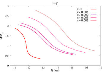
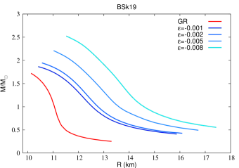
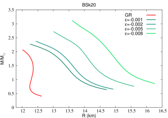
In Figs. 1–4, the diagram for various values of is represented. Herein some popular equations of state are used, namely Sly, BSK19, BSK20 and BSK21 respectively hp2004 ; potekhin13 . It is clear to see that for there is a significant deviation with respect to General Relativity. Noteworthy is the fact that, for increasingly large values of , the diagrams assume a self-similar behaviour. Larger radii and masses are achieved for negative values of the scaling parameter while, in the case of positive values, the traces are bent with usual General Relativity TOV equations. It is straightforward to see that we can reach masses about using the BSK20 and BSK21 equations of state.
A final comment is in order at this point. The radius in the figures has not to be identified with the constant of motion. The constant of motion fixes the functional relation between the mass M and the radius R saying that there is a characteristic gravitational radius which coincides with the Schwarzschild radius of General Relativity, i.e. for . Clearly, for any the gravitational radius changes. The integration constant can be chosen equal to 1 without affecting the system. The sign of is related to the relation. If larger stars can be achieved with respect to General Relativity. For , we obtains smaller stars.

V Conclusions
The mass of a self-gravitating system can be considered as a Noether charge according to the existence of the Noether symmetries.
In this paper, we derived both the conserved quantities and the functional form of gravity according to the so-called Noether Symmetry Approach cimento .
The final output is that a power-law form of gravity is determined by the Noether vector.
The power can be any real number.
Such a parameter is useful in order to study deviations with respect to General Relativity.
In particular, spherically-symmetric solutions are considered and we derived the field equations parameterized by .
Starting from this scheme, modified TOV equations are obtained and, assuming reliable equations of state discussed in the literature, the relation is achieved.
According to the value and the sign of , it is possible to show that radii and masses of compact neutron stars change with respect to General Relativity. This fact allows, in principle, that larger/smaller objects can be obtained by varying the gravitational sector with respect to those provided by the standard theory.
In particular, extremely large objects could be framed depending on modified gravity asta .
Some considerations are in order at this point.
The first is related to the Noether symmetries. The associated conserved quantity leads the relation. In other words, the existence of the symmetry is capable of ruling the stellar parameters and then the position of the star on the Hertzsprung-Russell diagram. In a general sense, the whole diagram could depend on the given theory of gravity and compact objects, where strong field effects are effective, could be
a useful testbed to retain or rule out alternative models.
Another consideration is related to the role of gravity in this framework. It seems that the parameter can really point out deviations with respect General Relativity emerging at given interaction lengths. Such lengths, depending on , has a similar role of the Schwarzschild radius (derived for ). The paradigm is that any theory of gravity has its own characteristic gravitational radius that can be something else with respect to the standard one of General Relativity. It is worth noticing that for small deviation with respect to General Relativity we can write
| (32) |
and then control the magnitude of the corrections with respect to the standard Hilbert-Einstein action. Such deviation could come out in the strong field regimes inside compact objects that could be very similar to some situations present in the early universe where logarithmic corrections emerge from quantization of curved space timeasta ; Starobinsky80 .
Finally, neutron stars, achieved in such a framework, could really discriminate between modified gravity and dark matter scenarios: in fact no exotic particle is requested in this context. The only natural assumption is that a symmetry breaking of gravitational interaction can happen at a given scale and energy, exactly like in the case of Starobinsky model of early universe where higher order curvature terms like give rise to inflation libroSV ; Starobinsky80 .
The Noether Symmetry Approach deserves some further general considerations. As firstly discussed in cimento , the utility of the method is twofold. From one hand, it allows to find out exact solutions since the presence of Noether symmetries reduces the related dynamical systems. Clearly, if the number of symmetries coincides with the number of dimensions of configuration space, the system is completely integrable. On the other hand, as shown here, the approach allows to select the class of models, in this case the power-law form of gravity. This means that the further degrees of freedom of any modified theory of gravity (scalar tensor, vector tensor, and so on) can be linked to the symmetries that rule the dynamics (see cimento for scalar tensor gravity). In this perspective, the Noether Symmetry Approach is a general criterion to select viable theories of gravity.
Acknowledgments
The Author is supported by the Grant "BlackHoleCam" Imaging the Event Horizon of Black Holes awarded by the ERC in 2013 (Grant No. 610058). The Author acknowledges the COST Action CA15117 (CANTATA) and INFN Sez. di Napoli (Iniziative Specifiche QGSKY and TEONGRAV).
References
- (1) J. Antoniadis et al. Science 340, 6131 (2013).
- (2) P. B. Demorest, T. Pennucci, S. M. Ransom, M. S. E. Roberts and J. W. T. Hessels, Nature 467, 1081 (2010).
- (3) S. Capozziello, M. De Laurentis, Phys. Rept. 509, 167 (2011).
- (4) S. Nojiri, S. D. Odintsov, Phys. Rept. 505, 59 (2011).
- (5) S. Nojiri, S. D. Odintsov, Int. J. Geom. Meth. Mod. Phys. 4, 115 (2007).
- (6) S. Capozziello, M. Francaviglia, Gen. Rel. Grav. 40, 357 (2008).
- (7) S. Capozziello, M. De Laurentis, V. Faraoni, The Open Astr. Jour , 2, 1874 (2009).
- (8) G. J. Olmo, Int. J. Mod. Phys. D 20, 413 (2011).
- (9) S. Capozziello and V. Faraoni, Beyond Einstein gravity: A Survey of gravitational theories for cosmology and astrophysics. Fundamental Theories of Physics. 170. Springer. (2010), ISBN 978-94-007-0164-9.
- (10) S. Capozziello and M. De Laurentis, Invariance Principles and Extended Gravity: Theories and Probes, Nova Science Publishers, Inc. (2010) ISBN: 978-1-61668-500-3.
- (11) T. P. Sotiriou and V. Faraoni, Reviews of Modern Physics 82, 451 (2010).
- (12) Y. Cai, S. Capozziello, M. De Laurentis, E.N. Saridakis, Rept. Prog. Phys. 79 106901 (2016).
- (13) S. Capozziello and M. De Laurentis, Scholarpedia, 10(2), 31422 (2015).
- (14) S. Capozziello and M. De Laurentis, Annalen der Physik 524, 545 (2012).
-
(15)
A. Astashenok, S. Capozziello, S. Odintsov, JCAP 12, 040 (2013);
A. Astashenok, S. Capozziello, S. Odintsov, Phys. Rev. D 89, 103509 (2014);
A. Astashenok, S. Capozziello, S. Odintsov, Astrophys. Space Sci. 355, 2182 (2014);
A. Astashenok, S. Capozziello, S. Odintsov, JCAP 01 001 (2015). - (16) P. Fiziev, Phys. Rev. D 87, 044053 (2013); P. Fiziev, arXiv:1402.2813v1 [gr-qc] (2014); P. Fiziev, PoS (FFP14) 080 (2014); P. Fiziev, K. Marinov, arXiv:1412.3015v1 [gr-qc] (2014).
- (17) J.D. Barrow and A.C. Ottewill, J.Phys. A 16, 2757 (1983).
- (18) N. Stergioulas, Living Rev. Rel. 6, 3 (2003).
- (19) R. Farinelli, M. De Laurentis, S. Capozziello, S.D. Odintsov, MNRAS 440, 3, 2894 (2014).
- (20) S. Capozziello, M. De Laurentis, S.D. Odintsov, A. Stabile, Phys. Rev. D 83, 064004 (2011).
- (21) S. Capozziello, M. De Laurentis, I. De Martino, M. Formisano, S.D. Odintsov, Phys. Rev. D 85, 044022 (2012).
- (22) S. Capozziello, M. De Laurentis, R. Farinelli, S.D. Odintsov, Phys. Rev. D 93, 023501 (2016).
- (23) S. Capozziello, A. Stabile and A. Troisi, Phys. Rev. D 76 104019 (2007).
- (24) S. Capozziello and S. Vignolo, Int. J. Geom. Meth. Mod. Phys. 6, 985 (2009).
- (25) S. Capozziello, R. de Ritis, C. Rubano, P. Scudellaro, Riv. Nuovo Cim. 19N4, 1 (1996).
- (26) S. Capozziello, Int. J. Mod. Phys. D 11 483 (2002); De Laurentis, Mod. Phys. Lett. A 30, 1550069 (2015); M. De Laurentis, M. Paolella, S. Capozziello, Phys. Rev. D 91, 083531 (2015); S: Capozziello, M. De Laurentis, S.D. Odintsov Mod. Phys. Lett. A 29, 1450164 (2014); S. Capozziello and M. De Laurentis, Int. J. Geom. Methods Mod. Phys. 11, 1460004 (2014); S. Capozziello and G. Lambiase, Gen. Relativ. Gravit. 32, 295 (2000); S. Capozziello, M. De Laurentis, R. Myrzakulov, Int. J. Geom. Methods Mod. Phys. 12, 1550095 (2015); S. Capozziello, M. De Laurentis, and R. Myrzakulov, Int. J. Geom. Methods Mod. Phys. 12, 1550065 (2015).
- (27) S. Capozziello, A. Stabile, A. Troisi Class. Quant. Grav. 24, 2153 (2007); S. Capozziello, M. De Laurentis, A. Stabile, Class.Quant.Grav. 27, 165008 (2010).
- (28) M. De Laurentis, R. De Rosa, F. Garufi, and L. Milano, Mon. Not. R. Astron. Soc. 424, 2371 (2012).
- (29) T. Clifton and J. D. Barrow, Phys. Rev. D 72, 103005 (2005).
- (30) S. Capozziello, M. De Laurentis, and M. Francaviglia, Astropart. Phys. 29, 125 (2008).
- (31) S.Weinberg "Gravitation and Cosmology", John Wiley & Sons, Inc., New York, (1972).
- (32) P. Haensel and A.Y. Potekhin, A&A, 428, 191 (2004).
- (33) A.Y. Potekhin, A.F. Fantina, N. Chamel, J.M. Pearson, S. Goriely, A&A, 560, A48 (2013).
- (34) A.A. Starobinsky, Phys. Lett. B 991, 99 (1980).