Role of flow of information in the speedup of quantum evolution

Abstract

The quantum evolution can be accelerated in non-Markovian environment. Previous results showed that the formation of system-environment bound state governs the quantum speedup. Although a stronger bound state in the system-environment spectrum may seem like it should cause greater speed of evolution, this seemingly intuitive thinking may not always be correct. We illustrate this by investigating a qubit driven by a classical field and coupled to a photonic crystal waveguide in the presence of a mirror. The perfect mirror can force part of the emitted light to return back to the qubit, and thus induce non-Markovian dynamics. Within the considered model, we show how the evolution speed is influenced by the memory time and the classical driving strength. In particular, we find that the formation of bound state is not the essential reason for the acceleration of evolution. The quantum speedup is attributed to the flow of information, regardless of the direction in which the information flows. Our conclusion can also be used to other non-Markovian environments.

PACS number(s)

03.65.Ud,03.65.Yz,03.67.Mn

I Introduction

The quantum evolution speed determines how quickly a quantum system needs to evolve between an initial state and a target state in a given process. Realization of controllable speeding up of evolution of a quantum system plays a key role in many technological applications, such as suppressing decoherence Georgescu153 and improving the efficiency of quantum computation Caneva240501 ; Lloyd1047 . For closed quantum systems, it has been shown that the entanglement can accelerate the quantum evolution Frowis052127 ; Batlr032337 . Due to the inevitable interaction between any system and its environment, a considerable amount of work has witnessed research on controlling speedup in more general open systems recently. One important discovery is that the non-Markovian process induced by the memory effect of environment can induce dynamical acceleration Defner010402 ; xu012307 , and therefore lead to a smaller quantum speed limit time (QSLT), which is defined as the minimal evolution time between two states Mandelstam249 ; Margolus188 . This phenomenon has been proved by the experiment in cavity QED systems Cimmarusti233602 .

Much effort has been made to explore how to exploit the non-Markovian environment itself to speed up quantum evolution. Some methods have been provided to speed up quantum evolution for open systems, such as by engineering multiple environments mo1600221 , driving the system by an external classical field zhang032112 , and using the periodic dynamical decoupling pulse Song43654 . The reason of quantum speedup for the above methods is found to be the increase of the degree of non-Markovianity. Recently, the authors of Re. Liu020105 showed that both the non-Markovianity and the quantum speedup are attributed to the formation of system-environment bound state, i.e., the stationary state of the whole system with eigenvalues residing in the band gap of energy spectrum Yablonovitch2059 ; zhu2136 ; tong052330 . If the bound state is established, the evolution of system becomes non-Markovian, and thus the quantum speedup happens. A good example of this is the situation where a two-level atom is coupled to an environment with a Ohmik spectrum. For this model, it has been found that providing stronger bound states can lead to higher degree of non-Markovianity, and hence to greater speed of quantum evolution Liu020105 . Based on this monotonic relation between the three, controlling speedup through manipulation of system-environment bound state has recently been studied behzzdi052121 . In some sense, one may intuitively think that the formation of bound state can be seen as the essential reflection to the speedup of quantum evolution. However, the mechanism for quantum speedup in non-Markovian quantum systems is still poorly understood if the environment is much complex.

The purpose of this paper is to examine the relationship between the formation of bound state, non-Markovianity and the quantum speedup. To do so, we consider a classical-driven atom coupled to a single-end one-dimensional (1D) photonic crystal (PC) waveguide. The end of the PC waveguide can be seen as a perfect mirror, forcing part of the emitted light to return back to the atom. The feedback behavior may induce the information backflow, i.e., the non-Markovian dynamics Breuer210401 . This structure has been used to develop single-photon transistors Chang807 and atomic light switches Zhou100501 . In this setting, the speedup process for the embedded atom can be acquired by manipulation of the classical driving field and the memory time of the environment. As for the mechanism of quantum speedup, some unexpected and nontrivial results are found. The formation of bound state can indeed lead to the non-Markovian evolution, but does not necessarily result in quantum speedup. The speedup of quantum evolution is attributed to the flow of information, regardless of the direction of information flows. We illustrate that it is not the amount of backflow information, i.e., the non-Markovianity, but the information flow volume that ultimately determines the actual speed of quantum evolution.

The work is organized as follows. The physical model is given in Section II. In Section III, we construct the measure of actual speed of quantum evolution based on information geometric formalism. Then we use this measure to investigate how the environment affect the speed of quantum evolution within our model in Section IV. In order to clarify the mechanism for quantum speedup, we first explore the interrelationship between the formation of bound state, non-Markovianity and the quantum speedup in Section V, and then present the role of the flow of information in the speeding up of evolution in Section VI. We summarize our results in Section VII.

II Physical model

We consider a qubit (two-level atom) with frequency $\omega_{0}$ driven by a classical field with frequency $\omega_{L}$. The qubit is embedded in a planar PC platform john2418 ; john12772 comprising a semi-infinite 1D waveguide along $x$-axis (see Fig. 1). The 1D waveguides, whose end lies at $x=0$, are coupled to the driven qubit at $x=x_{0}$. By neglecting the counter-rotating terms, the Hamiltonian is ($\hbar=1$)

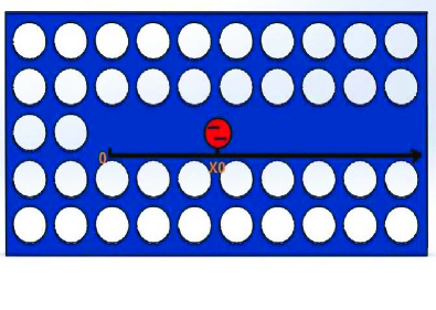
Figure 1: The implementation of the model. A single-end PC waveguide, whose end lies at $x=0$, is coupled to a two-level atom (qubit) at $x=x_{0}$.

$$H=\frac{\omega_{0}}{2}\sigma_{z}+\sum_{k}\omega_{k}a_{k}^{\dagger}a_{k}$$

$$+\Omega\left(e^{-i\omega_{L}t}\sigma_{+}+H.c.\right)+\sum_{k}(g_{k}a_{k}^{+}\sigma_{-}+H.c.),$$ (1)

where $\Omega$ is the coupling constant between the qubit and the classical field, $\sigma_{z}=\left|e\right\rangle\left\langle e\right|-\left|g\right\rangle\left\langle g\right|$ and $\sigma_{+}=\sigma_{-}^{\dagger}=\left|e\right\rangle\left\langle g\right|$ are the inversion and raising operators of the qubit with excited and ground states $\left|e\right\rangle$ and $\left|g\right\rangle$, $a_{k}$ ($a_{k}^{\dagger}$) is the annihilation (creation) operator for the $k$th field mode with frequency $\omega_{k}$, and $g_{k}$ is the coupling strength between the qubit and the $k$th mode.

The termination of the PC waveguide imposes a hard-wall boundary condition on the field, and that the part of emitted photon of the qubit will perform a round trip between the termination and the qubit. Thus the waveguide termination can be considered a perfect mirror. This semi-infinite 1D structure can provide a broad quantum optical properties Tufarelli013820 ; Horak459 .

In this model, the photon dispersion relationship around the atomic frequency is of the form Shen2001

$$\omega_{k}=\omega_{0}+\upsilon(k-k_{0}),$$ (2)

where $\upsilon$ is the photon group velocity, and $k_{0}$ is the carrier wave vector with $\omega_{k0}=\omega_{0}$. The coupling strength $g_{k}$ can be given by Tufarelli012113

$$g_{k}=\sqrt{\Gamma\upsilon/\pi}\sin kx_{0}$$ (3)

with the spontaneous emission rate $\Gamma$ of the qubit. For convenience of calculations, we first give the effect Hamiltonian of our model. By using the unitary transformation $U=\exp(-i\omega_{L}\sigma_{z}t/2)$, the Hamiltonian in Eq. (1) can be transferred to

$$H=\frac{\Delta}{2}\sigma_{z}+\Omega\sigma_{x}+\sum_{k}\omega_{k}a_{k}^{\dagger}a_{k}+\sum_{k}(g_{k}a_{k}^{+}\sigma_{-}e^{-i\omega_{L}t}+H.c.),$$ (4)

where $\Delta=\omega_{0}-\omega_{L}$. In the basis $\{\left|+\right\rangle=\cos\frac{\eta}{2}\left|e\right\rangle+\sin\frac{\eta}{2}\left|g\right\rangle,\left|-\right\rangle=-\sin\frac{\eta}{2}\left|e\right\rangle+\cos\frac{\eta}{2}\left|g\right\rangle\}$ with $\eta=\tan^{-1}(2\left|\Omega\right|/\Delta)$, the first two terms on the right hand side of the above equation can be diagonalized, and then the effect Hamiltonian can be rewritten as

$$H_{eff}=\frac{\omega_{ef}}{2}\xi_{z}+\sum_{k}\omega_{k}a_{k}^{\dagger}a_{k}+\sum_{k}(G_{k}a_{k}^{+}\xi_{-}+H.c.),$$ (5)

where $\omega_{ef}=\sqrt{\Delta^{2}+4\left|\Omega\right|^{2}}$, $G_{k}=\cos^{2}\frac{\eta}{2}g_{k}$, $\xi_{+}=\xi_{-}^{\dagger}=\left|+\right\rangle\left\langle-\right|$ and $\xi_{z}=\left|+\right\rangle\left\langle+\right|-\left|-\right\rangle\left\langle-\right|$.

At zero temperature, let us consider that the qubit is in the state $\left|+\right\rangle$ and the reservoir in the vacuum state $\left|\tilde{0}\right\rangle$. By the Hamiltonian described in Eq. (5), the state vector of the system at any time $t$, in the interaction picture, can be given by

$$\left|\varphi\left(t\right)\right\rangle=c_{+}\left(t\right)\left|+,\tilde{0}\right\rangle+\sum_{k}c_{k}\left(t\right)\left|-,\tilde{1}_{k}\right\rangle,$$ (6)

where the state $\left|\tilde{1}_{k}\right\rangle$ accounts for the field mode with frequency $\omega_{k}$ having one excitation. By using the Schrőinger equation, the amplitudes $c_{+}\left(t\right)$ and $c_{k}\left(t\right)$ are governed by

$$\dot{c}_{+}\left(t\right)=-i\sum_{k}G_{k}e^{i\left(\omega_{ef}-\omega_{k}\right)t}c_{k}\left(t\right),$$ (7)

$$\dot{c}_{k}\left(t\right)=-iG_{k}c_{+}\left(t\right)e^{-i\left(\omega_{ef}-\omega_{k}\right)t}.$$ (8)

By formal time integration of Eq. (8) and substituting this into the Eq. (7), the amplitude $c_{+}\left(t\right)$ can be transferred to

$$\dot{c}_{+}\left(t\right)=-\int_{0}^{t}dt^{{}^{\prime}}f(t-t^{{}^{\prime}})c_{+}\left(t^{{}^{\prime}}\right)$$ (9)

with $f(t-t^{{}^{\prime}})=\underset{k}{\sum}\left|G_{k}\right|^{2}e^{i(\omega_{ef}+\omega_{L}-\omega_{k})(t-t^{{}^{\prime}})}$. Through integrating of the correlation function $f(t-t^{{}^{\prime}})$ over $k$ and replacing this into Eq. (9), we acquire

$$\dot{c}_{+}\left(t\right)=-\cos^{4}\frac{\eta}{2}\frac{\Gamma}{2}c_{+}\left(t\right)$$

$$+\cos^{4}\frac{\eta}{2}\frac{\Gamma}{2}e^{i\left(\omega_{ef}-\Delta\right)t_{d}}e^{i\phi}c_{+}\left(t-t_{d}\right)\Theta\left(t-t_{d}\right),$$ (10)

where $\Theta\left(t\right)$ is the Heaviside step function and $\phi=2k_{0}x_{0}$.  $t_{d}=2x_{0}/\upsilon$ is such that the finite time taken by a photon to perform a round trip between qubit and the mirror, which behaves as an environmental memory time Tufarelli012113 . Obviously, the phase $\phi$ and the memory time $t_{d}$ are all dependent on the atomic embedded position $x_{0}$, which can be accurately controlled in the experiment Vats043808 . Performing the Laplace transformation of Eq. (10), we acquire

$$\tilde{c}_{+}\left(s\right)=\frac{1}{s+\cos^{4}\frac{\eta}{2}\frac{\Gamma}{2}-\cos^{4}\frac{\eta}{2}\frac{\Gamma}{2}e^{i(\omega_{x}t_{d}+\phi)}e^{-st_{d}}},$$ (11)

where $\omega_{x}=\omega_{ef}-\Delta.$ By inverting the Laplace transform, we can obtain trung2524

$$c_{+}\left(t\right)=e^{-\cos^{4}\frac{\eta}{2}\frac{\Gamma}{2}t} \sum\frac{1}{n!}(\cos^{4}\frac{\eta}{2}\frac{\Gamma}{2}e^{i\omega_{x}t_{d}}e^{i\phi}e^{\cos^{4}\frac{\eta}{2}\frac{\Gamma}{2}t_{d}})^{n}$$ (12)

$$\cdot(t-nt_{d})^{n}\Theta\left(t-nt_{d}\right),$$

where the dynamical evolution is witnessed by the memory time $t_{d}$.

III Measure of dynamical speed

The quantum speed of dynamical evolution can be constructed by applying the method of differential geometry BengtssonBook . Taking the perspective of this method, the set of quantum states is indeed a Riemannian manifold, that is the set of density operators over the Hilbert space. The geometric length between the given initial state $\rho_{0}$ and the final state $\rho_{\tau}$ can be naturally measured by using possible Reimannian metrics over the manifold. According to the theorem of the Morozova, Čencov and Petz theorem Morozova2648 ; petz221 ; toth032324 , any monotone Riemannian metric can be given by the unified form

$$g^{f}\left(A,B\right)=\frac{1}{4}Tr\left(Ac\left(L_{\rho},R_{\rho}\right)B\right),$$ (13)

where $A$ and $B$ are any hermitian operators, and $c\left(x,y\right)$ is a symmetric function defined as

$$c\left(x,y\right)=\frac{1}{yf(x/y)}$$ (14)

with $f(t)$ being the Morozova-Čencov (MC) function which fulfills $f(t)=tf(1/t)$ and $f(1)=1$ Kubo205 . The MC function is related to our chosen Riemannian metric, that is different forms of MC functions stand for different Reimannian metrics. $L_{\rho}$ and $R_{\rho}$ are two linear superoperators defined as $L_{\rho}A=\rho A$ and $R_{\rho}A=A\rho$.

Given the unified form of Riemannian metric, the squared infinitesimal length between two neighboring quantum states $\rho$ and $\rho+d\rho$ can be given by petz81

$$ds^{2}=g^{f}\left(d\rho,d\rho\right).$$ (15)

Here, we consider a dynamical evolution with a map $\Lambda_{t}$. The evolved state is $\rho_{t}=\Lambda_{t}\rho_{0}$ with a initial state $\rho_{0}$. Along the evolved path between $\rho_{0}$ and $\rho_{\tau}$ with $t\in[0,\tau]$, the line element of the path can be expressed as

$$dl=\sqrt{g^{f}\left(\partial_{t}\rho_{t},\partial_{t}\rho_{t}\right)}dt.$$ (16)

Then, the instantaneous speed of quantum evolution can be given by

$$V=\frac{dl}{dt}=\sqrt{g^{f}\left(\partial_{t}\rho_{t},\partial_{t}\rho_{t}\right)}.$$ (17)

The average speed between time zero and $\tau$ is

$$V_{a}=\frac{1}{\tau}\int_{0}^{\tau}Vdt.$$ (18)

In order to obtain the measure of dynamical speed in an explicit form, we can rewrite the evolved state $\rho_{t}$ in the form of its spectral decomposition, $\!\rho_{t}\!=\!\underset{k}{\sum}p_{k}\left|\phi_{k}\right\rangle\left\langle\phi_{k}\right|\!$, with $0\!<\!p_{k}\!<\!1$ and $\underset{k}{\sum}p_{k}\!=\!1$. According to the Morozova-Čencov-Petz formalism, the instantaneous speed can be rewritten as BengtssonBook

$$V=\sqrt{\underset{k}{\sum}\frac{\left|\dot{p_{k}}\right|^{2}}{4p_{k}}+\underset{k\neq l}{\sum}c(p_{k},p_{l})\frac{p_{k}(p_{k}-p_{l})}{2}\left|\left\langle\phi_{l}|\dot{\phi_{k}}\right\rangle\right|^{2}}.$$ (19)

Clearly, any contractive Riemannian metric can be employed to evaluate the speed of evolution with different type of MC function $f(t)$. As shown by Re. Kubo205 , a generic MC function must fulfill $f_{\min}(t)<f(t)<f_{\max}(t)$, where $f_{\min}(t)=2t/(1+t)$ and $f_{\max}(t)=(1+t)/2$. Interestingly, an intermediate MC function with $f_{WY}(t)=(1+\sqrt{t})^{2}/4$ and $c_{WY}(x,y)=4/\left(\sqrt{x}+\sqrt{y}\right)^{2}$ is the one corresponding to the Wigner-Yanase information metric, which is widely used in detecting the speed of dynamical evolution Deza2014 . In what follows, we focus on the Wigner-Yanase information metric. Other potential appropriate metric is straightforward.

IV Controllable of quantum speedup

In this section, we apply the measure constructed above to the 1D waveguide system, and study the mechanism for controllable speedup. We consider the atomic system is initially in an arbitrary pure state $\left|\Psi\left(0\right)\right\rangle=\beta\left|+\right\rangle+\sqrt{1-\beta^{2}}\left|-\right\rangle$ $\left(0\leq\beta\leq 1\right)$, and the reservoir is in the vacuum state $\left|\tilde{0}\right\rangle$. Exploiting Eq. (6), the reduced density matrix for the qubit can be calculated as (in the basis $\left\{\left|+\right\rangle,\left|-\right\rangle\right\}$)

$$\rho_{a}\left(t\right)=\left(\begin{array}[]{cc}\beta^{2}P_{t}&\beta\sqrt{1-\beta^{2}}\sqrt{P_{t}}\\ \beta\sqrt{1-\beta^{2}}\sqrt{P_{t}}&1-\beta^{2}P_{t}\end{array}\right),$$ (20)

where $P_{t}=\left|c_{+}\left(t\right)\right|^{2}$ denotes the excited state population of the qubit. The spectral decomposition of $\rho_{a}\left(t\right)$ can be expressed as the form

$$\rho_{a}\left(t\right)=\sum_{k=\pm}p_{k}\left|\phi_{k}\right\rangle\left\langle\phi_{k}\right|,$$ (21)

with $\!p_{\pm}\!=\!\left(1\!\pm\!\lambda\right)/2\!$ and $\!\left|\phi_{\!\pm\!}\right\rangle\!=\!\left(\alpha_{\pm}\left|\!+\!\right\rangle+\left|-\right\rangle\right)/\sqrt{1\!+\!\alpha_{\pm}^{2}}$, where $\!\lambda\!=\!\sqrt{1\!-\!4\beta^{2}P_{t}\!+\!4\beta^{4}P_{t}^{2}}$ and $\alpha_{\pm}\!=\!\left(2\beta^{2}P_{t}\!\pm\!\lambda\!-\!1\right)/\left(2\beta\sqrt{1-\beta^{2}}\sqrt{P_{t}\!}\right)$.

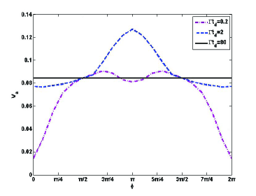
Figure 2: The average speed of quantum evolution $V_{a}$ between the time zero and $\Gamma\tau=10$ (in units of $1/\Gamma$) as a function of phase $\phi$ for various values of memory time $\Gamma t_{d}$ with $\Omega=0$, $\Delta=0$ and $\beta=1$.

The dynamics of the qubit is fully determined by the Eq. (10). Clearly, the first term on the right side of Eq. (10) is corresponding to the atomic spontaneous emission. While the second term represents the effect of the presence of the mirror on the atomic dynamical evolution.  For the sake of clarity, in what follows we consider three cases corresponding to the regimes of small, intermediate and vary large values of $\Gamma t_{d}$, respectively.

A. The small value of $\Gamma t_{d}$

For simplicity, we first consider the case where there is no classical field, i.e., the driving strength $\Omega=0$. Fig. 2 shows the average speed between the time zero and $\Gamma\tau=10$ (in units of $1/\Gamma$) for the system as a function of phase $\phi$. We can find that, in the regime where the memory time is small with $\Gamma t_{d}=0.2$, the normalized average speed for the qubit system is always relatively small. The maximum value of $V_{a}$ is not exceed $0.1$ in the range $\phi\in\left[0,2\pi\right]$.

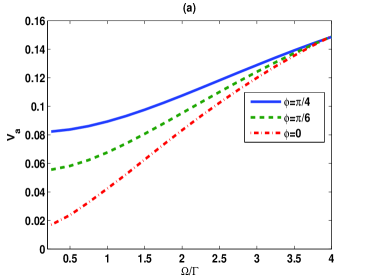
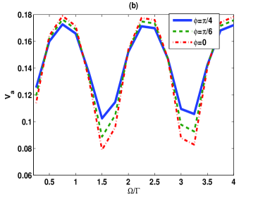
Figure 3: The average speed of quantum evolution $V_{a}$ between the time zero and $\Gamma\tau=10$ as a function of classical driving strength $\Omega$ (in units of $1/\Gamma$) for various values of phase $\phi$ with $\Delta=0$ and $\beta=1$. (a) The memory time is small with $\Gamma t_{d}=0.2$. (b) The memory time is intermediate with $\Gamma t_{d}=2$.

In order to obtain the speedup of quantum evolution in this case, we show how the classical field influence the speed of the qubit. The variation of $V_{a}$ with respect to driving strength $\Omega$ for different $\phi$ is plotted in Fig. 3(a). For each line with a fixed $\phi$, the increase of driving strength $\Omega$ leads to an increase of the average speed. So, we therefore reach the interesting result that the classical field can be used to speed up the dynamical evolution in the case of the memory time is small.

B. The intermediate value of $\Gamma t_{d}$ 

The regime of intermediate value of $\Gamma t_{d}$ means that the memory time is shorter than the atomic spontaneous emission time, but can not be ignored. In this situation, the qubit will undergo standard spontaneous emission up to time $t=t_{d}$, which is independent of the phase $\phi$. After that, the presence of the mirror begins to affect the dynamics of the open system. The fraction of light emitted by the qubit will be reflected back to the qubit. So the presence of the mirror is fully responsible for the non-Markovian character. In this case, the speed of the atomic dynamical evolution is different from the above case, where the small memory time dose not induce any non-Markovianity Tufarelli012113 . As shown from Fig. 2 (dashed line), over the entire range of the phase $\phi$, the average speed in the intermediate regime ($\Gamma t_{d}=2)$ is bigger than the case where the memory time is small. An interesting feature here is that the speed $V_{a}$ has the obvious periodicity change under action of the driving strength (as shown in Fig. 3(b)). That is to say, in the intermediate regime, the speed of dynamical evolution can be controlled to a speed-up and speed-down process by the classical driving strength.

C. The regime of very large value of $\Gamma t_{d}$ 

It is worth noting the situation where the memory time is very large ($\Gamma t_{d}\gg 1$). In this case, the memory time is so large that the emitted photon can not be reflected by the waveguide end, even when the qubit has decayed to the ground state. Also, the dynamical evolution occurs independently of the phase $\phi$ and the classical field. This is due to the fact that the back-reflected light cannot recombine with the light emitted towards the end of the waveguide and no interference takes place. Thus, as expected, the average speed exhibits a plateau independent of $\phi$, as shown in Fig. 2 (solid line).

In concluding this section, we would like to emphasize that, the classical field as well as the the memory time $t_{d}$ play an important role in controlling speedup. One can simply control the memory time (i.e., the position of the embedded atom) and the driving strength to accelerate dynamical evolution on demand. Our proposed scheme is experimentally accessible. In experiment, the planar photonic crystal can be prepared by a GaAs PC membrane, and the qubit can be prepared by the self-assembled InGaAs QDs with a lower density Yoshie200 . We can use the method of electron beam lithography to construct the photonic-crystal 1D waveguide. Furthermore, the recent experiment has demonstrated an excellent control on the atomic embedded position by the method of electrohydrodynamic jet printing See051101 . By this way, we can verify our prediction.

V Relationship between formation of bound state, non-Markovianity and quantum speedup

Previous result shows that Liu020105 the formation of the system-environment bound state is the essential reason of the quantum speedup. It is demonstrated that providing stronger bound states can lead to higher degree of non-Markovianity, and hence to greater speed of quantum evolution. In order to understand the physical reason of the speedup in our model, we further study the interrelation between the formation of bound state, the non-Markovianity and the speed of quantum evolution.

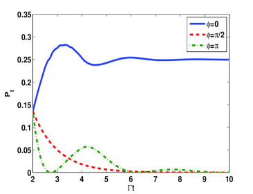
Figure 4: The atomic excited population $P_{t}$ as a function of $\Gamma t$ for various values of phase $\phi$ with $\Gamma t_{d}=2$, $\beta=1$, $\Delta=0$ and $\Omega=0$. Note that only the range $t>t_{d}$ is shown due to the fact that the behavior exhibits an exponential decay and does not dependent on $\phi$ in $t<t_{d}$.

The system-environment bound state is actually the stationary state of the whole system liu052139 . The formation of the bound state can lead to the inhibition of spontaneous emission, i.e., the system holds an amount of excitation in long time. Furthermore, the more stronger the bound state is, the greater the amount of excitation bounded around the system is. This phenomenon has been demonstrated in super-Ohmic Tong155501 and photonic crystals bath John4083 . For our two-level atomic system, the formation of bound state can be detected by the excited state population $P_{t}$ wu431 , which is sketched in Fig. 4. Obviously, it can be confirmed that, if $\phi=\pi/2$, population decreases monotonically to zero, implying that the bound state is absent. However, if $\phi=0,$ the population maintains a steady-state value in long time limit. This population trapping behavior means that fraction of light emitted by the qubit can only penetrate a distance given by the length between the qubit and the mirror, and then be reflected back to the qubit, forming the atom-photon bound state. While in the case $\phi=\pi$, the bound state is established but it is not stronger than the case that $\phi=0$. Thus, $P_{t}$ exhibits a periodically decrease, that is only a small amount of excitation reflected back to the qubit in this case.

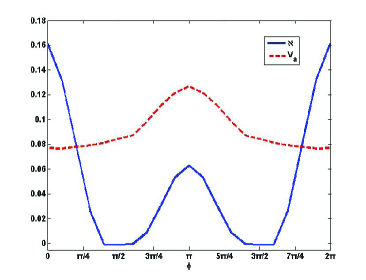
Figure 5: The non-Markovianity $\aleph$ (solid line) and the average speed $V_{a}$ (dashed line) as a function of phase $\phi$ with $\Gamma t_{d}=2$, $\Omega=0$, $\Delta=0$ and $\beta=1$.

In Fig. 5, we sketch the behaviors of non-Markovianity $\aleph$ and the speed $V_{a}$. The measure of non-Markovianity for our model is shown in the Appendix. We can find that the non-Markovianity connects directly with the formation of bound state. When the bound state is established, such as in the case where $\phi=0$, the system presents non-Markovian effect with $\aleph>0.$ However, once the bound state is absent with $\phi=\pi/2$, the behavior of sudden transition from non-Markovian to Markovian effect ($\aleph=0$) occurs. This result confirms the previous result that the non-Marikovianity is attributed to the formation of bound states Liu020105 .

Now we focus on the speed of quantum evolution. When the bound state is established and becomes stronger, the Markovian approximation of the environment fails and one might expect the memory effect to accelerate the speed of evolution. This would be true if one were considering a simple model where the qubit is directly connected to a reservoir taking Lorentzian or Ohmic structures, as shown in Re behzzdi052121 . However, this relation may not be universally true. When we considering our much complex physical model where a classical driven qubit is confined in a controllable photonic waveguide, a particularly astonishing phenomenon occurs. As shown in Fig. 5, when the bound state is established with $\phi=0$ and the maximum non-Markovianity, the average speed is $V_{a}=0.078$. While in the case where $\phi=\pi/2$ and $\aleph=0$ (Markovian effect), we can acquire $V_{a}=0.088$, which is bigger than the case, where the non-Markovianity is maximum in the range $\phi\in\left[0,2\pi\right]$.

Thus, the surprising message is that a stronger system-environment bound state may not always helpful in enhancing the speed of quantum evolution. What is the mechanism of speedup in a memory environment? What can be seen as an essential reflection to the speedup of quantum evolution? To answer the above questions, in the next section we further investigate the speedup from the perspective of the direction of flow of information in memory environments.

VI Mechanism for the controlling speedup of quantum evolution

The non-Markovian effect of environment connects tightly with the flow direction of information. This is because the accepted notion of non-Markovianity is based on the idea that the environment would cause the information backflow from environment to the system for non-Markovian process, while for Markovian process, the information flows in only one direction, that is from the system to the environment, with no feedback Breuer210401 . The flow direction of information can be monitored by the changing rate of the trace distance, i.e., $\sigma\left(t,\rho_{1,2}\left(0\right)\right)=\frac{d}{dt}D\left(\rho_{1}\left(t\right),\rho_{2}\left(t\right)\right)$. The rate $\sigma\left(t,\rho_{1,2}\left(0\right)\right)$ is positive for an information backflow from environment to the system, and negative for the information flowing in the opposite direction. Based on this, the total amount of backflow information $\aleph=$ $\underset{\rho_{1,2}\left(0\right)}{\max}\int_{\sigma>0}dt\sigma\left(t,\rho_{1,2}\left(0\right)\right)$ is defined as the degree of non-Markovianity (see the Appendix).

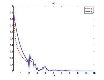
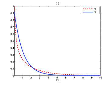
Figure 6: The instantaneous speed $V$ (dashed line) and the absolute value of information changing rate $\Re=\left|\sigma\left(t,\rho_{1,2}\left(0\right)\right)\right|$ (solid line) as a function of $\Gamma t$ for (a) $\phi=0$ and (b)$\phi=\pi/2$ with $t_{d}=2,\Omega=0and\Delta=0$.

Previous studies have shown that non-Markovian effect can speed up quantum evolution. However, the degree of non-Markovianity $\aleph$ could not be seen as an essential reflection to the quantum speedup. That is to say the reason for the speedup is not solely to the backflow information. One question naturally arise: What is the effect of the information flowing from system to environment on quantum evolution?

Next, we focus on this question. In terms of above analysis, the total amount of flow information consisting the flow from system to environment and the reverse flow is determined by

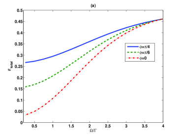
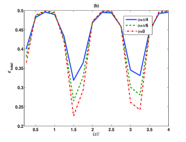
Figure 7: The total amount of flow information $\aleph_{total}$ between the time zero and the time $\Gamma t=10$ as a function of classical driving strength $\Omega$ for various values of phase $\phi$ with $\Delta=0$. (a) The memory time is small with $\Gamma t_{d}=0.2$. (b) The memory time is intermediate with $\Gamma t_{d}=2$.

$$\aleph_{total}=\underset{\rho_{1,2}\left(0\right)}{\max}\int dt\Re(t),$$ (22)

where the absolute value of changing rate $\Re(t)=\left|\sigma\left(t,\rho_{1,2}\left(0\right)\right)\right|$ denotes the flowing of information. The comparison of the changing rate $\Re(t)$ and the instantaneous speed $V$ for various values of phase $\phi$ with a fixed memory time is shown in Fig. 6. It is interesting to find that the changing rate $\Re(t)$ exhibits the same behavior as the speed of quantum evolution. That is, the increase (decrease) of $\Re(t)$ leads to an increase (a decrease) of instantaneous speed of quantum evolution. We thus conjecture that the flowing of information plays a key role in controlling the speed of quantum evolution. In order to further study the mechanism of controllable speeding up of the evolution within the considered model, we plot in Fig. 7 the total amount of flow information $\aleph_{total}$ as a function of classical driving strength $\Omega$ for various values of phase $\phi$. By contrasting the $\aleph_{total}$ and the average speed shown in Fig. 3, the results also confirm that the driving strength can increase the information flow volume $\aleph_{total}$, and thus accelerate the quantum speed of evolution. We therefore reach the interesting conclusion that it is the flow of information that directly affects the quantum speed of evolution, regardless of the direction of information flows. That is why in some cases, the Markovian precess ($\aleph=0$) can also enhance the speed of evolution, as shown in Fig. 5.

VII Conclusion

In summary, we have studied a classical driven qubit that is coupled to an 1D photonic-crystal waveguide. We have investigated how the external classical driving strength and the reservoir’s memory time affect the quantum speed of evolution. We find that, with a judicious choice of the driving strength of the applied classical field, the speedup of evolution can be achieved in both Markovian (the memory time is small) and non-Markovian (the memory time is intermediate) processes. We have also explored the mechanism of well-controlled quantum speedup in our model. Surprisingly, a stronger system-reservoir bound state with a higher degree of non-Markovianity does not necessarily result in a greater speed of quantum evolution. More specifically, within the considered model, we have shown that it is not the amount of backflow information, i.e., the non-Markovianity, but the total amount of flow information that directly affect the average evolution speed for some interval of time. Our study sheds further light on the interplay between information flowing and the evolution speed of an open quantum system.

Finally, it should be note that our conclusion applies not only to the above model, but also to situations like a qubit coupled to a environment with Lorentzian or Ohmic structure. Within these models, it is easy to check that population trapping will not be happened Defner010402 ; Liu020105 ; behzzdi052121 . The population $P_{t}$ exhibits a monotonic decay (Markovian dynamics) or a periodically decrease (mon-Markovian dynamics). The difference of speed between the Markovian and non-Markovian cases, i.e., the difference of the total amount of flow information ($\aleph_{total}$) between them, is mainly determined by the backflow information. The effect of the information flowing from system to environment can be ignored. Thus, the non-Markovianity becomes the unique reason for quantum speedup in these models.

VIII Acknowledgements

This work was supported by the the Young Foundation of Shan Dong province (Grant number ZR2017QA002) and Doctoral Foundation of University of Jinan (Grant no. XBS1325).

Appendix A Measure of non-Markovianity

In non-Markovian dynamics, the environment would cause the information backflow from environment to the system. The non-Markovianity describing the total amount of backflow information is defined as

$$\aleph=\underset{\rho_{1,2}\left(0\right)}{\max}\int_{\sigma>0}dt\sigma\left(t,\rho_{1,2}\left(0\right)\right),$$ (23)

where $\sigma\left(t,\rho_{1,2}\left(0\right)\right)=\frac{d}{dt}D\left(\rho_{1}\left(t\right),\rho_{2}\left(t\right)\right)$ denotes the changing rate of the trace distance $D\left(\rho_{1}\left(t\right),\rho_{2}\left(t\right)\right)=\frac{1}{2}tr\left|\rho_{1}(t)-\rho_{2}(t)\right|$ between states $\rho_{1,2}(t)$ evolving from their respective initial states $\rho_{1,2}\left(0\right)$ Breuer210401 . The dynamical process is non-Markovian if there exists a pair of initial states and at certain time such that $\sigma\left(t,\rho_{1,2}\left(0\right)\right)>0$. For our two-level system, the optimal pair of initial states has been proven to be $\rho_{1,2}\left(0\right)=\left|\pm\right\rangle\left\langle\pm\right|$ Wissmann062108 . Then the trace distance can be acquired $D\left(\rho_{1}\left(t\right),\rho_{2}\left(t\right)\right)=\left|c_{+}\left(t\right)\right|^{2}$.

References

- (1) I. M. Georgescu, S. Aahhab, and F. Noir, Rev. Mod. Phys. 86, 153 (2014).
- (2) T. Caneva, M. Murphy, T. Calarco, R. Fazio, S. Montangero, V. Giovannetti, and G. E. Santoro, Phys. Rev. Lett. 103, 240501 (2009).
- (3) S. Lloyd, Nature (London) 406, 1047 (2000).
- (4) F. Frowis, Phys. Rev. A 85, 052127 (2012).
- (5) J. Batle, M. Casas, A. Plastino, and A. R. Plastino, Phys. Rev. A 72, 032337 (2005).
- (6) S. Deffner and E. Lutz, Phys. Rev. Lett. 111, 010402 (2013).
- (7) Z. Y. Xu, S. Luo, W. L. Yang, C. Liu, and S. Zhu, Phys. Rev. A 89, 012307 (2014).
- (8) L. Mandelstam and I. Tamm, J. Phys. (USSR) 9, 249 (1945).
- (9) N. Margolus and L. B. Levitin, Phys. D 120, 188 (1998).
- (10) A. D. Cimmarusti, Z. Yan, B. D. Patterson, L. P. Corcos, L. A. Orozco, and S. Deffner, Phys. Rev. Lett. 114, 233602 (2015).
- (11) M. L. Mo, J. Wang, and Y. N. Wu, Ann. Phys. (Berlin) 529, 1600221 (2017).
- (12) Y. J. Zhang, W. Han, Y. J. Xia, J. P. Cao, and H. Fan, Phys. Rev. A 91, 032112 (2015).
- (13) Y. J. Song, Q. S. Tan, and L. M. Kuang, Sci. Rep. 7, 43654 (2017).
- (14) H. B. Liu, W. L. Yang, J. H. An, and Z. Y. Xu, Phys. Rev. A 93, 020105(R) (2016).
- (15) E. Yablonovitch, Phys. Rev. Lett. 58, 2059 (1987).
- (16) S. Y. Zhu, Y. Yang, H. Chen, H. Zheng, and M. S. Zubairy, Phys. Rev. Lett. 84, 2136 (2000).
- (17) Q. J. Tong, J. H. An, H. G. Luo, and C. H. Oh, Phys. Rev. A 81, 052330 (2010).
- (18) N. Behzadi, B. Ahansaz, A. Ektesabi, and E. Faizi, Phys. Rev. A 95, 052121 (2017).
- (19) H. P. Breuer, E. M. Laine, and J. Piilo, Phys. Rev, Lett. 103, 210401 (2009).
- (20) D. E. Chang, A. S. SØensen, E. A. Demler, and M. D. Lukin, Nat. Phys. 3, 807 (2007).
- (21) L. Zhou, Z. R. Gong, Y. X. Liu, C. P. Sun, and F. Nori, Phys. Rev. Lett. 101, 100501 (2008).
- (22) S. John and J. Wang, Phys. Rev. Lett. 64, 2418 (1990).
- (23) S. John and J. Wang, Phys. Rev. B 43, 12772 (1991).
- (24) T. Tufarelli, F. Ciccarello, and M. S. Kim, Phys. Rev. A 87, 013820 (2013).
- (25) P. Horak, P. Domokos, and H. Ritsch, Europhys Lett. 61, 459,(2003).
- (26) J. T. Shen and S. H. Fan, Opt Lett. 30, 2001 (2005).
- (27) T. Tufarelli, M. S. Kim, and F. Ciccarello, Phys. Rev. A 90, 012113 (2014).
- (28) N. Vats, S. John, and K. Busch, Phys. Rev. A 65, 043808 (2002).
- (29) H. T. Dung and K. Ujihara, Phys. Rev. A 59, 2524 (1999).
- (30) I. Bengtsson and K. Zyczkowski, Geometry of Quantum States: An Introduction to Quantum Entanglement (Cambridge University Press, England, 2006).
- (31) E. A. Morozova and N. N. Cencov, J. Sov. Math. 56, 2648 (1991).
- (32) D. Petz and H. Hasegawa, Lett. Math. Phys. 38, 221 (1996).
- (33) F. Hiai and D. Petz, Algeb. Appl. 430, 3105 (2009).
- (34) F. Kubo and T. Ando, Math. Ann. 246, 205 (1980).
- (35) D. Petz, Lin. Algeb. Appl. 244, 81 (1996).
- (36) M. M. Deza and E. Deza, Encyclopedia of Distances,(Springer-Verlag, Berlin Heidelberg, 2014).
- (37) T. Yoshie, et al. Nature 432, 200 (2004).
- (38) G. G. See, L. Xu, E. Sutanto, A. G. Alleyne, R. G. Nuzzo, and B. T. Cunningham, Appl. Rhys. Lett 107, 051101 (2015).
- (39) H. B. Liu, J. H. An, C. Chen, Q. J. Tong, H. G. Luo, and C. H. Oh, Phys. Rev. A 87, 052139 (2013).
- (40) Q. J. Tong, J. H. An, H. G. Lu, and C. H. Oh, J. Phys. B 43 155501 (2010).
- (41) S. John and T. Quang, Phys. Rev. A 52, 4083 (1995).
- (42) Y. N. Wu, J. Wang, and H. Z. Zhang, Opt. Commun. 366, 431 (2016).
- (43) S. Wissmann, A. Karlsson, E. M. Laine, J. Piilo, and H. P. Breuer, Phys. Rev. A 86, 062108 (2012).