Sparse Network Estimation for Dynamical Spatio-temporal Array Models

Abstract

Neural field models represent neuronal communication on a population level via synaptic weight functions. Using voltage sensitive dye (VSD) imaging it is possible to obtain measurements of neural fields with a relatively high spatial and temporal resolution. The synaptic weight functions represent functional connectivity in the brain and give rise to a spatio-temporal dependence structure. We present a stochastic functional differential equation for modeling neural fields, which leads to a vector autoregressive model of the data via basis expansions of the synaptic weight functions and time and space discretization. Fitting the model to data is a pratical challenge as this represents a large scale regression problem. By using a 1-norm penalty in combination with localized basis functions it is possible to learn a sparse network representation of the functional connectivity of the brain, but still, the explicit construction of a design matrix can be computationally prohibitive. We demonstrate that by using tensor product basis expansions, the computation of the penalized estimator via a proximal gradient algorithm becomes feasible. It is crucial for the computations that the data is organized in an array as is the case for the three dimensional VSD imaging data. This allows for the use of array arithmetic that is both memory and time efficient.The proposed method is implemented and showcased in the R package dynamo available from CRAN.

1 Introduction

Neural field models are models of aggregated membrane voltage of a large and spatially distributed population of neurons. The neuronal network is determined by spatio-temporal synaptic weight functions in the neural field model, and we will refer to these weight functions as the propagation network. This network determines how signals are propagated hence it is of great interest to learn the propagation network from experimental data, which is the inverse problem for neural field models.

The literature on neural fields is vast and we will not attempt a review, but see Bressloff (2012); Coombes et al. (2014) and the references therein. The typical neural field model considered is a deterministic integrodifferential equation. The inverse problem for the deterministic Amari equation was treated in beim Graben and Potthast (2009) and Potthast and beim Graben (2009), and stochastic neural field models was, for instance, treated in Chapter 9 in Coombes et al. (2014) and in Faugeras and Inglis (2015). One main contribution of the latter paper, Faugeras and Inglis (2015), was to treat a stochastic version of the Amari equation in the well developed theoretical framework of functional stochastic evolution equations.

Despite the substantial literature on neural fields, relatively few papers have dealt directly with the estimation of neural field components from experimental data. Pinotsis et al. Pinotsis et al. (2012) demonstrated how a neural field model can be used as the generative model within the dynamical causal modeling framework, where model parameters can be estimated from electrophysiological data. The modeling of voltage sensitive dye (VSD) imaging data in terms of neural fields was discussed in Chemla and Chavane (2010), and Markounikau et al. Markounikau et al. (2010) estimated parameters in a neural field model directly from VSD data.

In this paper, VSD imaging data is considered as well. This in vivo imaging technique has a sufficiently high resolution in time and space to detect propagation of changes in membrane potential on a mesoscopic scale, see Roland et al. (2006). A prevalent notion in the neuroscience literature is that the network connecting the neurons, and through which brain signals are propagated, is sparse, and that the propagation exhibits a time delay. If a spiking neuron, for instance, only affects neurons via synaptic connections to a very localized region the network is spatially sparse, while connections to remote regions result in temporal sparsity and long range dependence, see, e.g., Brunel (2000); Sporns et al. (2004); Roxin and Montbrió (2011); Bressloff and Webber (2012); Touboul (2014). Finally the possibility of feedback waves in the brain, e.g., as suggested in Roland et al. (2006), could also be explained by spatio-temporal dynamics depending on more than just the instantaneous past. These considerations lead us to suggest a class of stochastic neural field models that allows for time delay, and a proposed estimation methodology that provides sparse nonparametric estimation of synaptic weight functions. Thus we do not make assumptions about spatial homogeneity or isotropy of the functional connectivity, nor do we assume that the signal propagation is instantaneous.

In order to derive a statistical model that, from a computational viewpoint, is feasible for realistically sized data sets, a time and space discretized version of the infinite dimensional dynamical model is obtained by replacing the various integrals with Riemann-Itô type summations and relying on an Euler scheme approximation. This approximation scheme makes it possible to derive a statistical model with an associated likelihood function such that regularized maximum-likelihood estimation becomes computationally tractable. Especially, we show that by expanding each component function in a tensor product basis we can formulate the statistical model as a type of multi-component linear array model, see Lund et al. (2017).

The paper is organized as follows. First we give a brief technical introduction to the stochastic dynamical model that form the basis for the paper. Then we present the aggregated results from the application of our proposed estimation methodology to part of a VSD imaging data set. The remaining part of the paper presents the derivation of the linear array model and the key computational techniques required for the actual estimation of the model using array data. The appendix contains further technical proofs, a meta algorithm and implementation details. Finally to further illustrate our results we also provide a Shiny app available at shiny.science.ku.dk/AL/NetworkApp/ as well as supplementary material, Lund and Hansen (2018), containing results from fitting the model to individual trials and the aggregated result for the entire data set.

2 A stochastic functional differential equation

The data that we will ultimately consider is structured as follows. With $\tau,T>0$, $\mathcal{T}\coloneqq[-\tau,T]$ and $N_{x},N_{y},M,L\in\mathbb{N}$ we record, to each of $N_{t}\coloneqq M+L+1$ time points

$$-\tau=t_{-L}<\ldots<t_{0}<\ldots<t_{M}=T,$$ (1)

a 2-dimensional rectangular $N_{x}\times N_{y}$ image of neuronal activity in an area of the brain represented by the Cartesian product $\mathcal{S}\coloneqq\mathcal{X}\times\mathcal{Y}\subseteq\mathbb{R}^{2}$. These images consist of $D\coloneqq N_{x}N_{y}$ pixels each represented by a coordinate $(x_{i},y_{j})$ lying on a grid ${\mathbb{G}}^{2}\subseteq\mathcal{S}$. To each time point each pixel has a color represented by a value $\boldsymbol{v}(x_{i},y_{j},t_{k})\in\mathbb{R}$. Thus the observations are naturally organized in a 3-dimensional array $\boldsymbol{v}\coloneqq\{\boldsymbol{v}(x_{i},y_{j},t_{k})\}_{i,j,k}$ where the first two dimensions correspond to the spatial dimensions and the third dimension corresponds to the temporal dimension.

As such it is natural to view $\boldsymbol{v}$ as a discretely observed sample in time and space of an underlying spatio-temporal random field $\boldsymbol{V}$. Following Definition 1.1.1 in Adler and Taylor (2009) any measurable map $\boldsymbol{V}:\Omega\to\mathbb{R}^{\mathcal{R}}$, with $\mathcal{R}\subseteq\mathbb{R}^{d},d\in\mathbb{N}$, a parameter set, is called a $(d,1)$-random field or simply a $d$-dimensional random field. Especially, for the brain image data, $\boldsymbol{V}$ is real valued with a 3-dimensional parameter set $\mathcal{R}\coloneqq\mathcal{S}\times\mathcal{T}$ where $\mathcal{S}$ refers to space while $\mathcal{T}$ refers to time. We emphasize the conceptual asymmetry between these dimensions by calling $\boldsymbol{V}$ a spatio-temporal random field. For fixed $t$, as $\boldsymbol{V}(t)\coloneqq\boldsymbol{V}(\cdot,\cdot,t):\mathbb{R}^{2}\to\mathbb{R}$ this model will inevitably be a stochastic dynamical model on a function space, that is an infinite dimensional stochastic dynamical model.

Following the discussion in the introduction above we propose to model the random neural field $\boldsymbol{V}$ via a stochastic functional differential equation (SFDE) with the propagation network incorporated into the drift as a spatio-temporal linear filter (a convolution) with an impulse-response function (convolution kernel) quantifying the network. The solution to the SFDE in a Hilbert space ${\mathcal{H}}$ is then the underlying time and space continuous model $\boldsymbol{V}$ for the data $\boldsymbol{v}$.

To introduce the general model more formally let $(\Omega,{\mathcal{F}},\Pr)$ be a probability space endowed with an increasing and right continuous family $({\mathcal{F}}_{t})$ of complete sub-$\sigma$-algebras of ${\mathcal{F}}$. Let ${\mathcal{H}}$ be a reproducing kernel Hilbert space (RKHS) of continuous functions over the compact set $\mathcal{S}\times\mathcal{S}$. Suppose $(\boldsymbol{V}(t))_{t}$ is a continuous ${\mathcal{F}}_{t}$-adapted, ${\mathcal{H}}$-valued stochastic process and let ${\mathcal{C}}\coloneqq{\mathcal{C}}([-\tau,0],{\mathcal{H}})$ denote the Banach space of continuous maps from $[-\tau,0]$ to ${\mathcal{H}}$. Then $(\boldsymbol{V}_{t})_{t}$, where

$$\boldsymbol{V}_{t}\coloneqq\{\boldsymbol{V}(t+s)\}_{s\in(-\tau,0)},\quad t\geq 0,$$ (2)

defines a ${\mathcal{C}}$-valued stochastic process over $\mathbb{R}_{+}$. We call $\boldsymbol{V}_{t}$ the $\tau$-memory of the random field $\{\boldsymbol{V}(r)\}_{r\in\mathcal{S}\times\mathcal{T}}$ at time $t\geq 0$.

Let $\mu:{\mathcal{C}}\times[0,T]\to{\mathcal{H}}$ be a bounded linear operator and consider the stochastic functional differential equation (SFDE) on ${\mathcal{H}}$ given by

$$\mathrm{d}\boldsymbol{V}(t)=\mu(\boldsymbol{V}_{t},t)\mathrm{d}t+\mathrm{d}\boldsymbol{W}(t).$$ (3)

Here $\boldsymbol{W}$ is a spatially homogenous Wiener process with spectral measure $\sigma$ ($\sigma$ is a finite symmetric measure on $\mathbb{R}^{2}$) as in Peszat and Zabczyk (1997). That is, $\boldsymbol{W}$ is a centered Gaussian random field such that $\{W(x,y,t)\}_{t}$ is a $({\mathcal{F}}_{t})_{t}$-Wiener process for every $(x,y)\in\mathbb{R}^{2}$, and for $t,s\geq 0$ and $(x,y),(x^{\prime},y^{\prime})\in\mathbb{R}^{2}$

$$\mathrm{E}\{\boldsymbol{W}(x,y,t)\boldsymbol{W}(x,^{\prime}y^{\prime},s)\}=(t\land s)c(x-x^{\prime},y-y^{\prime}).$$ (4)

Here $c:\mathbb{R}^{2}\to\mathbb{R}$, the covariance function defined as the Fourier transform of the spectral measure $\sigma$, quantifies the spatial correlation in $\boldsymbol{W}$.

Compared to a typical SDE, the infinitesimal dynamic at time $t$ as described by (3) depends on the past via the $\tau$-memory of $V$ in the drift operator $\mu$. Hence processes satisfying (3) will typically be non-Markovian. We note that all the memory in the system is modelled by the drift $\mu$.

The non-Markovian property makes theoretical results regarding existence, uniqueness and stability of solutions to (3) much less accessible. Corresponding to Section 0.2 in Da Prato and Zabczyk (2014), in order to obtain theoretical results, it should be possible to lift the equation (3) and obtain a Markovian SDE on the Banach space ${\mathcal{C}}$. Consequently an unbounded linear operator (the differential operator) then appears in the drift. It is outside the scope of this paper to pursue a discussion of the theoretical properties of (3). General theoretical results on SDEs on Banach spaces are not abundant, see, e.g., Cox (2012), where SDEs and especially SDDEs on Banach spaces are treated. Especially, Corollary 4.17 in Cox (2012) gives an existence result for a strong solution to (3). Also in Xu et al. (2012) a mild existence results are given for an SDDE on a Hilbert space and for the specification introduced next this result can be strengthened to a strong solution result. In general, the requirements for a solution to exist is, corresponding to the finite dimensional case, that the coefficient operators are Lipschitz continuous, which, e.g., the integral operator presented next satisfies.

2.1 Drift operator

The idea here is that the drift operator $\mu$ will capture both external input to the system (the brain in our context) as well as the subsequent propagation of this input over time and space. By decomposing the drift operator we obtain drift components responsible for modelling instantaneous effects and propagation effects respectively. To this end we will specify the drift operator by the decomposition

$$\mu(\boldsymbol{V}_{t},t)\coloneqq\mathrm{S}(t)+\mathrm{F}(\boldsymbol{V}_{t})+\mathrm{H}\{\boldsymbol{V}(t)\}.$$ (5)

Here $\mathrm{S}:\mathcal{T}\to{\mathcal{H}}$, $\mathrm{S}(t)(x,y)\coloneqq s(x,y,t)$, with $s\in L^{2}(\mathbb{R}^{3},\mathbb{R})$ a smooth function of time and space, models a deterministic time dependent external input to the system. $\mathrm{H}:{\mathcal{H}}\to{\mathcal{H}}$, $\mathrm{H}\{\boldsymbol{V}(t)\}(x,y)\coloneqq h(x,y)\boldsymbol{V}(x,y,t)$ where $h\in{\mathcal{H}}$, a smooth function of space, captures the short range (infinitesimal) memory in the system.

The long range memory responsible for propagating the input to the system over time and space is modelled by the operator $\mathrm{F}:{\mathcal{C}}([0,\tau],{\mathcal{H}})\to{\mathcal{H}}$ given as the integral operator

$$\mathrm{F}(\boldsymbol{V}_{t})(x,y)=\int_{\mathcal{S}}\int_{-\tau}^{0}w(x,y,x^{\prime},y^{\prime},r)\boldsymbol{V}(x^{\prime},y^{\prime},t+r)\mathrm{d}r\mathrm{d}x^{\prime}\mathrm{d}y^{\prime}.$$ (6)

Here $w\in L^{2}(E^{5},\mathbb{R})$ is a smooth weight function quantifying the impact of previous states on the current change in the random field $\boldsymbol{V}$. Especially, the value $w(x,y,x^{\prime},y^{\prime},r)$ is the weight by which the change in the field at location $(x,y)$ is impacted by the level of the field at location $(x^{\prime},y^{\prime})$ with delay $r$. With this specification, a solution to (3), if it exists, can be written in integral form as

$$\boldsymbol{V}(x,y,t)=\int_{0}^{t}\bigg{\{}s(x,y,u) +\int_{\mathcal{S}}\int_{-\tau}^{0}w(x,y,x^{\prime},y^{\prime},r)\boldsymbol{V}(x^{\prime},y^{\prime},u+r)\mathrm{d}r\mathrm{d}x^{\prime}\mathrm{d}y^{\prime}$$

$$+h(x,y)\boldsymbol{V}(u)\bigg{\}}\mathrm{d}{}u+\int_{0}^{t}\mathrm{d}\boldsymbol{W}(x,y,u)\mathrm{d}{}u.$$ (7)

Thus (2.1) characterizes a solution to a stochastic delay differential equation (SDDE) on ${\mathcal{H}}$ with delays distributed over time and space (spatio-temporal distributed delays) according to the impulse-response function $w$. We can think of $w$ as quantifying a spatio-temporal network in the brain that governs how the propagation of the input is to be distributed over time and space, and we will refer to $w$ as the network function.

Standard neural field models usually include a non-linear transformation of $\boldsymbol{V}$, via a so-called gain function, inside the integral operator $\mathrm{F}$. It is possible to include a known gain function transformation in (2.1) without substantial changes to our proposed methodology for estimating $s$, $w$ and $h$. However, to the best of our knowledge the appropriate choice of gain function for empirical data has not been settled. It is, of course, possible to attempt to estimate the gain function from data as well, but to avoid complicating matters we proceed by regarding (2.1) as corresponding to a linearization of the unknown gain function. We note that the interpretation of $w$ will always be relative to the choice of gain function, and it might not quantitatively represent physiological properties of the brain, if the gain function is misspecified.

Next we present an example where a statistical model based on the spatio-temporal SDDE model proposed above is fitted to real high dimensional brain image data. The derivation of this statistical model relies on a space time discretization and is discussed in Section 4. We note that key elements in our approach involves expanding the network function (along with the other component functions) using basis functions with compact support in time and space domain. We then apply regularization techniques to obtain a sparse (i.e., space-time localized) estimate of the network.

3 Brain imaging data

The data considered in this section consists of in vivo recordings of the visual cortex in ferret brains provided by Professor Per Ebbe Roland. In the experiment producing the data, a voltage sensitive dye (VSD) technique was used to record a sequence of images of the visual cortex, while presenting a visual stimulus, a stationary white square displayed for 250 ms on a grey screen, to the ferret. Each recording or trial is thus a film showing activity in a live ferret brain before, during and after a visual stimulus is presented. The purpose of the experiment was to study the response in brain activity to the stimulus and its propagation over time and space.

For each of a total of 13 ferrets the experiment was repeated several times producing a large-scale spatio-temporal data set with 10 to 40 trials pr. ferret resulting in 275 trials (films) in total. Each trial contains between 977 and 1720 images with time resolution equal to 0.6136 ms pr. image. For this particular data set each image was recorded using a hexagonal photodiode array with 464 channels and a spatial resolution equal to 0.15 mm pr. channel (total diameter is 4.2 mm), see Roland et al. (2006). The hexagonal array is then mapped to a $25\times 25$ rectangular array to yield one frame or image. This mapping in principle introduce some distortion of the image but we ignore that here and consider 0.15 mm pr. pixel to be the spatial resolution.

Here we present an aggregated fit obtained by first fitting the above model to all trials for animal 308 (12 trials) each consisting of 977 $25\times 25$ images. Then by mean aggregating these single trial fits we obtain one fit based on all trials for this animal. Note that each of the 12 single trial fits for animal 308 are visualized in Section 3 in the supplementary material. We have carried out this analysis for all 13 animals – the entire data set – and present the visualizations of the remaining 12 aggregated fits in Section 2 in the supplementary material. The estimation procedure and a snippet of the data is available from CRAN via the R package dynamo, see Lund (2018a).

For the analysis we let $L\coloneqq 50$ thus allowing a 31 ms delay. For each single trial (film) the model is fitted using a lasso regularized linear array model derived in Section 4 below. The lasso regression is carried out for 10 penalty parameters $\lambda_{1}>\ldots>\lambda_{10}>0$. Here we present the fit for model 6, i.e., $\lambda=\lambda_{6}$, which we selected using 4-fold cross validation on the 12 trials, see Section 1 in the supplementary material. For additional details about the specific regression setup see C.1.

3.1 The aggregated stimulus and network estimates

Fig. 1 shows the estimate of the stimulus for all pixels 69 ms after onset. We argue that the “high stimulus” areas visible in Fig. 1 correspond to the expected mapping of the center of field of view (CFOV), see Fig. 1 in Harvey et al. (2009).

For the pixel indicated with a white dot in the right panel of Fig. 1, we show the raw data for each trial along with the trial specific estimate of the stimulus component and the aggregated stimulus component in Fig. 2. Notice that the estimated stimulus component shows both an on-signal after the stimulus start and an off-signal after the stimulus stop. Also notice the considerable variation over trials in the raw data with some trials displaying a clear signal and others almost no signal.

Visualizing the aggregated estimate of the network is more challenging as this is quantified by the function $w:\mathbb{R}^{5}\to\mathbb{R}$. A Shiny app visualizing $w$ is available online (see shiny.science.ku.dk/AL/NetworkApp/), and here we present various time and space aggregated measures of propagation effects – some of which are inspired by analogous concepts from graph theory.

In Fig. 3 below we plot the the fitted version of the two bivariate functions $w^{-},w^{+}:\mathbb{R}^{2}\to\mathbb{R}$ given by

$$w^{-}(x,y) \coloneqq\frac{1}{{\deg^{-}}(x,y)}\int_{\mathcal{S}}\int_{-\tau}^{0}|w(x,y,x^{\prime},y^{\prime},t)|\mathrm{d}{}t\mathrm{d}{}x^{\prime}\mathrm{d}{}y^{\prime},$$ (8)

$$w^{+}(x^{\prime},y^{\prime}) \coloneqq\frac{1}{{\deg^{+}}(x^{\prime},y^{\prime})}\int_{\mathcal{S}}\int_{-\tau}^{0}|w(x,y,x^{\prime},y^{\prime},t)|\mathrm{d}{}t\mathrm{d}{}x\mathrm{d}{}y$$ (9)

where

$$\deg^{-}(x,y) \coloneqq\int_{\mathcal{S}}\int_{-\tau}^{0}1_{\{w(x,y,x^{\prime},y^{\prime},t)\neq 0\}}\mathrm{d}{}t\mathrm{d}{}x^{\prime}\mathrm{d}{}y^{\prime}\quad$$

$$\deg^{+}(x^{\prime},y^{\prime}) \coloneqq\int_{\mathcal{S}}\int_{-\tau}^{0}1_{\{w(x,y,x^{\prime},y^{\prime},t)\neq 0\}}\mathrm{d}{}t\mathrm{d}{}x\mathrm{d}{}y,$$

are the aggregated non-zero effects going in to $(x^{\prime},y^{\prime})$ (indegree) respectively out from $(x,y)$ (outdegree). Here $w^{+}(x^{\prime},y^{\prime})$ quantifies the effect of $(x^{\prime},y^{\prime})$ on all other coordinates relative to the aggregated non-zero effects, that is time and space aggregated propagation effects from $(x^{\prime},y^{\prime})$. Similarly $w^{-}(x,y)$ quantifies time and space aggregated propagation effects to $(x,y)$. Mean aggregated estimates of these functions are shown in Fig. 3.

From bottom panel in Fig. 3 we see that an area is identified which across all pixels has a relatively great weight on other pixels across the 12 trials. Thus this area is identified by the model as important in the propagation of neuronal activity across trials. We notice that this high output as quantified by $w^{+}$ overlaps with the strongest of the two high stimulus areas (CFOV) in Fig. 2. Thus the estimated weight functions propagate primarily the direct stimulus signal.

From the top panel we see that the pixels receiving propagation effects on the other hand is more scattered around the cortex. However, the high input areas overlap with both of the high stimulus areas (CFOVs) in Fig. 2 suggesting the existence of a propagation network connecting the high stimulus area and the low stimulus area and the immediate surroundings of the high stimulus area.

Next for fixed $(x^{\prime},y^{\prime})$ consider quantifying the aggregated (in) effects from all points that lie $s$ spatial units away and that arrive with a delay of $t$ time units. Letting $p$ denote the polar coordinate parametrization of the $s$-sphere $S_{1}(s)$ in $\mathbb{R}^{2}$ with centre $(0,0)$,

$$p:[0,2\pi]\to S_{1}(s),$$

and compute the desired quantity for fixed $s,t,x^{\prime},y^{\prime}$ as a curve integral

$$\int_{S_{1}(s)}w(p+(x^{\prime},y^{\prime}),x^{\prime},y^{\prime},t)\mathrm{d}{}p=\int_{0}^{2\pi}w\{p_{1}(r)+x^{\prime},p_{2}(r)+y^{\prime},x^{\prime},y^{\prime},t\}|p^{\prime}(r)|\mathrm{d}{}r.$$

Integrating this over $\mathcal{S}$ we obtain a bivariate function

$$W(s,t)\coloneqq\int\bigg{\{}\int_{S_{1}(s)}w(p+(x^{\prime},y^{\prime}),x^{\prime},y^{\prime},t)\mathrm{d}{}p\bigg{\}}\mathrm{d}{}x^{\prime}\mathrm{d}{}y^{\prime}$$

giving the aggregated effects in the entire field as a function of spatial separation $s$ (Euclidian distance) and temporal separation (time delay) $t$.

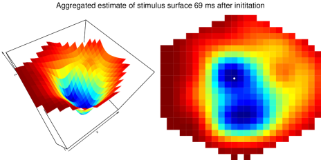
Figure 1: Mean aggregated estimate 69 ms after stimulus onset. The white dot in the right panel indicates the pixel visualized in Fig. 2.

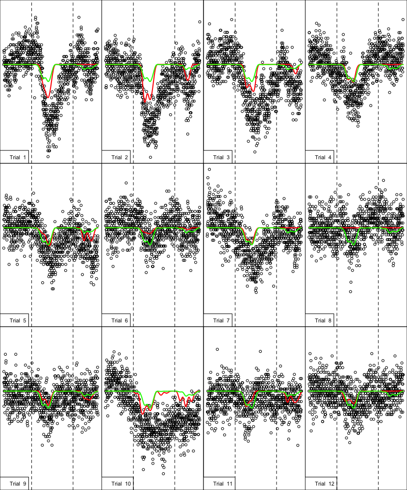
Figure 2: The data observed at pixel $(x,y)$ (indicated in Fig. 1) (black) and the estimate of $s(x,y,\cdot)$ for each trial (red) and the mean aggregated estimated (green). Dotted vertical lines indicate stimulus start and stop. Notice the considerable variation among the trials.

From bottom panel in Fig. 3 we see that an area is identified which across all pixels has a relatively great weight on other pixels across the 12 trials. Thus this area is identified by the model as important in the propagation of neuronal activity across trials. We notice that this high output as quantified by $w^{+}$ overlaps with the strongest of the two high stimulus areas (CFOV) in Fig. 2. Thus the estimated weight functions propagate primarily the direct stimulus signal.

From the top panel we see that the pixels receiving propagation effects on the other hand is more scattered around the cortex. However, the high input areas overlap with both of the high stimulus areas (CFOVs) in Fig. 2 suggesting the existence of a propagation network connecting the high stimulus area and the low stimulus area and the immediate surroundings of the high stimulus area.

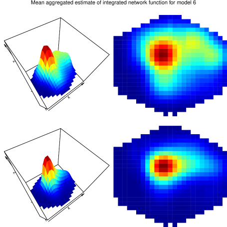
Figure 3: The aggregated weight functions $\hat{w}^{-}$ (top) and $\hat{w}^{+}$ (bottom).

Fig. 4 summarizes the network function as a function of temporal and spatial separation. The largest effects seem to occur with a delay of around 7 ms and has an effect on coordinates approximately 0–0.3 mm away. Especially the significant propagation effects do not seem to extend beyond 1.2 mm from the source and arrive with no more than 28 ms delay.

Finally, Fig. 5 shows a density plot of the estimated weight values in $\hat{w}$. The density plot is truncated as most weights are estimated to zero. From Fig. 5 we can see that the most frequent delay of the estimated effects is roughly 9 to 10 ms.

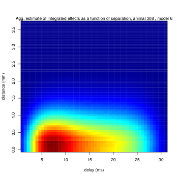
Figure 4: Plot of $\hat{W}$ quantifying the mean aggregated estimate of propagation effects as a function of temporal and spatial separation.

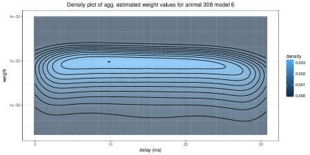
Figure 5: Truncated density plots of the estimated weight values.

4 A linear model

The statistical model underlying the inferential framework used to obtain the results in Section 3 is based on a discretized version of the SFDE (3). The first step in our approach is to discretize space by aggregating the field over small areas. Let $(\mathcal{S}_{m,n})_{m,n}\coloneqq(\mathcal{X}_{m}\times\mathcal{Y}_{n})_{m=1,n=1}^{N_{x},N_{y}}$ denote a partition of $\mathcal{S}$ with $D\coloneqq N_{x}N_{y}$ elements with size ${\rm Leb}(\mathcal{S}_{m,n})=\Delta_{s}>0$ for all $m,n$. We have from the integral representation of $\boldsymbol{V}$ in (2.1) that

$$\int_{\mathcal{S}_{m,n}}\boldsymbol{V}( x,y,t)\mathrm{d}{}x\mathrm{d}{}y=\int_{0}^{t}\bigg{\{}\int_{\mathcal{S}_{m,n}}s(x,y,u)\mathrm{d}{}x\mathrm{d}{}y$$

$$+\int_{-\tau}^{0}\sum_{i,j}\int_{\mathcal{S}_{i,j}}\boldsymbol{V}(x^{\prime},y^{\prime},u+r)\int_{\mathcal{S}_{m,n}}w(x,y,x^{\prime},y^{\prime},r)\mathrm{d}{}x\mathrm{d}{}y\mathrm{d}{}x^{\prime}\mathrm{d}{}y^{\prime}\mathrm{d}{}r$$

$$+\int_{\mathcal{S}_{m,n}}\boldsymbol{V}(x,y,u)h(x,y)\mathrm{d}{}x\mathrm{d}{}y\bigg{\}}\mathrm{d}{}u+\int_{\mathcal{S}_{m,n}}\int_{0}^{t}\mathrm{d}\boldsymbol{W}(x,y,u)\mathrm{d}{}x\mathrm{d}{}y.$$ (10)

Here as noted in Peszat and Zabczyk (1997) the last term for each $(x,y)$ is an Itô-integral with respect to a real valued Wiener process. Furthermore, using the covariance function for the random field from (4), the covariance of two such terms is

$$\mathrm{E}\bigg{\{}\int_{\mathcal{S}_{m,n}}\int_{0}^{t}\mathrm{d}\boldsymbol{W}(x,y,u)\mathrm{d}{}x\mathrm{d}{}y \int_{\mathcal{S}_{i,j}}\int_{0}^{t}\mathrm{d}\boldsymbol{W}(x,y,u)\mathrm{d}{}x\mathrm{d}{}y^{\prime}\bigg{\}}$$

$$=\int_{\mathcal{S}_{m,n}}\int_{\mathcal{S}_{i,j}}\mathrm{E}\{\boldsymbol{W}(x,y,t)\boldsymbol{W}(x^{\prime},y^{\prime},t)\}\mathrm{d}{}x^{\prime}\mathrm{d}{}y^{\prime}\mathrm{d}{}x\mathrm{d}{}y$$

$$=\int_{\mathcal{S}_{m,n}}\int_{\mathcal{S}_{i,j}}tc(x-x^{\prime},y-y^{\prime})\mathrm{d}{}x^{\prime}\mathrm{d}{}y^{\prime}\mathrm{d}{}x\mathrm{d}{}y.$$

We then apply a Riemann type approximation of the space integrals over the partition sets $\mathcal{S}_{m,n}$ on the left and the right of (4). This leads us to consider the $D$-dimensional real valued stochastic process denoted $\boldsymbol{\tilde{V}}$, with the $(m,n)$th entry process given by

$$\boldsymbol{\tilde{V}}_{m,n}(t)=\int_{0}^{t}\bigg{\{} \boldsymbol{\tilde{\mathrm{S}}}_{m,n}(u)$$

$$+\int_{-\tau}^{0}\sum_{i,j}\boldsymbol{\tilde{V}}_{i,j}(u+r)\int_{\mathcal{S}_{m,n}}w(x,y,x_{i},y_{j},r)\mathrm{d}{}x\mathrm{d}{}y\mathrm{d}{}r$$

$$+\boldsymbol{\tilde{\mathrm{H}}}_{m,n}\{\boldsymbol{\tilde{V}}(u)\}\bigg{\}}\mathrm{d}{}u+\int_{0}^{t}\mathrm{d}\boldsymbol{\tilde{W}}_{m,n}(u)\mathrm{d}u,$$ (11)

as a space discretized model for the random field $\boldsymbol{V}$, where $\boldsymbol{\tilde{\mathrm{S}}}_{m,n}(u)\coloneqq\Delta_{s}s(x_{m},y_{n},u)$ and $\boldsymbol{\tilde{\mathrm{H}}}_{m,n}\{\boldsymbol{\tilde{V}}(u)\}\coloneqq\Delta_{s}h(x_{m},y_{n})\boldsymbol{\tilde{V}}_{m,n}(u)$.

Notice that in (4) $\boldsymbol{\tilde{V}}(t)$ is an $N_{x}\times N_{y}$ matrix. However we might as well think of it as an $N_{x}N_{y}\times 1$ vector $\tilde{V}(t)$. When necessary we will distinguish between the matrix (array) form and the vector form using the following notation.

The mapping $[i_{1},\ldots,i_{d}]:\bigtimes_{j=1}^{d}\{1,\ldots,N_{i_{j}}\}\to\{1,\ldots,\prod_{j=1}^{d}N_{i_{j}}\}$ is a bijection, and for an array $\boldsymbol{A}\coloneqq\boldsymbol{\mathrm{(}}\boldsymbol{A}_{i_{1},\ldots,i_{d}})_{i_{1},\ldots,i_{d}}$ we denote the corresponding vector as ${A}_{[i_{1},\ldots,i_{d}]}=\boldsymbol{A}_{i_{1},\ldots,i_{d}}$. For $d=2$ we may take $[i_{1},i_{2}]:=i_{1}+(i_{2}-1)N_{i_{2}}$.

Using this notation let $\tilde{W}=\{(\tilde{W}_{[1,1]}(t),\ldots,\tilde{W}_{[N_{x},N_{y}]}(t))\}_{t}$ denote a $D$-dimen
-sional Brownian motion on $(\Omega,{\mathcal{F}},\Pr)$ adapted to $({\mathcal{F}}_{t})_{t}$ with covariance matrix $\tilde{C}$ having rows given by

$$\tilde{C}_{[m,n]}\coloneqq(c(x_{m}-x_{1},y_{n}-y_{1}),\ldots,c(x_{m}-x_{N_{x}},y_{n}-y_{N_{y}}))\Delta_{s}^{2},$$

for each $[m,n]\in\{1,\ldots,D\}$, then $\boldsymbol{\tilde{W}}$ with $\boldsymbol{\tilde{W}}_{i,j}=\tilde{W}_{[i,j]}$ is the array version appearing in (4).

Aggregating $\boldsymbol{V}$ over the spatial partition $(\mathcal{S}_{m,n})_{m,n}$ leads to a multi-dimen
-sional SDDE as an approximate model for our data. Such models are mathematically easier to handle compared to the random field model (2.1), see Mao (2007). Especially, we can obtain a discrete time approximation to the solution (4) using an Euler scheme following Buckwar and Shardlow (2005). The proof is in A.

Proposition 1.

Let $(t_{k})_{k=-L}^{M}$ with $\Delta_{t}\coloneqq t_{k+1}-t_{k}>0$ denote a partition of $\mathcal{T}$. With $(\boldsymbol{w}_{\ell})_{\ell=-L}^{-1}$ a sequence of weight matrices depending on the network function $w$, the solution $(\tilde{\tilde{V}}_{k})_{k}$ to the forward Euler scheme

$$\tilde{\tilde{V}}_{k+1} -\tilde{\tilde{V}}_{k} =\bigg{\{}\tilde{\mathrm{S}}(t_{k})+\sum_{\ell=-L}^{-1}\boldsymbol{w}_{\ell}\tilde{\tilde{V}}_{k+\ell}+\tilde{\mathrm{H}}(\tilde{\tilde{V}}_{k})\bigg{\}}\Delta_{t}+\tilde{C}\sqrt{\Delta_{t}}\epsilon_{k},$$ (12)

where $(\epsilon_{k})_{k}$ are independent and $\mathcal{N}(0,I_{D})$ distributed, converges weakly to the (vectorized) solution $\tilde{V}$ to (4).

Note that for each $k$, $\tilde{\mathrm{S}}(t_{k})$ and $\tilde{\mathrm{H}}(\tilde{\tilde{V}}_{k})$ are just the vectorized versions of $\boldsymbol{\tilde{\mathrm{S}}}(t_{k})$ and $\boldsymbol{\tilde{\mathrm{H}}}(\boldsymbol{\tilde{\tilde{V}}}_{k})$ respectively with $\boldsymbol{\tilde{\tilde{V}}}$ the array version of ${\tilde{\tilde{V}}}$.

Next as the component functions; the stimulus functions $s$, the network function $w$ and the short range memory $h$, are assumed to be square integrable we can use basis expansions to represent them, i.e., for $p_{s},p_{w},p_{h}\in\mathbb{N}$,

$$s(x,y,t) =\sum_{q=1}^{p_{s}}\alpha_{q}\phi_{q}(x,y,t),$$ (13)

$$w(x,y,x^{\prime},y^{\prime},t) =\sum_{q=1}^{p_{w}}\beta_{q}\phi_{q}(x,y,x^{\prime},y^{\prime},t),$$ (14)

$$h(x,y) =\sum_{q=1}^{p_{h}}\gamma_{q}\phi_{q}(x,y).$$ (15)

where $(\alpha_{q})_{q}$, $(\beta_{q})_{q}$ and $(\gamma_{q})_{q}$ are three sets of basis coefficients and $(\phi_{q})_{q}$ is generic notation for a set of basis functions. We let $p\coloneqq p_{s}+p_{w}+p_{h}$ denote the total number of basis functions used. Using (13)-(15) we can formulate the dynamical model (12) as a vector autoregressive model. The proof is given in A.

Proposition 2.

There exists a $D\times 1$ vector $y_{k}$ and a $D\times p$ matrix $X_{k}$ such that we can write the dynamical model (12) as an autoregression

$$y_{k}=X_{k}\theta+e_{k},\quad k=0,\ldots,M-1$$ (16)

where $(e_{k})_{k}$ are i.i.d. $\mathcal{N}_{D}(0,\Sigma)$ with $\Sigma\coloneqq\tilde{C}^{\top}\tilde{C}\Delta_{t}$. Defining

$$y\coloneqq\left(\begin{array}[]{ccc}y_{1}\\ \vdots\\ y_{M}\end{array}\right),\quad X\coloneqq\left(\begin{array}[]{ccc}X_{1}\\ \vdots\\ X_{M}\end{array}\right),$$ (23)

the associated negative log-likelihood can be written as

$$\ell_{X}(\theta,\Sigma)=\frac{M}{2}\ln|\Sigma|+\big{\|}\big{(}I_{M}\otimes\Sigma^{-1/2}\big{)}(y-X\theta)\big{\|}_{2}^{2},$$ (24)

with $I_{M}$ the $M\times M$ identity matrix.

We note that due to the structure of the linear model (16) the MLEs of $\theta$ and $\Sigma$ are not available in closed form. Especially the normal equations characterizing the MLEs are coupled in this model leading to a generalized least squares type estimation problem. Furthermore, the $DM\times p$ design matrix $X$ will for realistically sized data become very large making it infeasible to fit the model (16) directly by minimizing (24) . Next we will discuss how to compute regularized estimates of the parameters $\theta$ and $\Sigma$ by exploiting the array structure of the problem to reformulate the autoregressive model (16) as a (partial) linear array model. This in turn makes the computations involved in the fitting procedure feasible.

4.1 Penalized linear array model

In order to obtain time and space localized estimates of the component functions, we will minimize a regularized version of (24). Letting $\Omega\coloneqq\Sigma^{-1}$ denote the precision matrix, this is achieved by solving the unconstrained problem

$$\min_{\theta\in\mathbb{R}^{p},\Omega\in M^{D\times D}}\ell_{X}(\theta,\Omega^{-1})+\lambda J_{1}(\theta)+\nu J_{2}(\Omega),$$ (25)

where $J_{1}$ and $J_{2}$ are convex penalty functions and $\lambda\geq 0$ and $\nu\geq 0$ the penalty parameters controlling the amount of regularization. For non-differentiable penalty functions $J_{i}$, $i=1,2$, solving (25) results in sparse estimates of $\theta$ and $\Omega$. In the following we will use the lasso or $\ell_{1}$ penalty, i.e., $J_{1}=J_{2}=\|\cdot\|_{1}$, see Tibshirani (1996).

Following Rothman et al. (2010) we solve (25) using their approximate MRCE algorithm. In our setup the steps are as follows:

1. For fixed $\hat{\Omega}$ and each penalty parameter $\lambda_{1}\geq\ldots\geq\lambda_{K}$, $K\in\mathbb{N}$, solve

   $$\min_{\theta\in\mathbb{R}^{p}}\ell_{X}(\theta,{\hat{\Omega}}^{-1})+\lambda_{i}J_{1}(\theta).$$ (26)

2. For $i\in\{1,\ldots,K\}$ let $\hat{\theta}_{\lambda_{i}}$ denote the estimate from step 1, let $\hat{\Sigma}_{R,i}\coloneqq(y-X\hat{\theta}_{\lambda_{i}})^{\top}(y-X\hat{\theta}_{\lambda_{i}})$ and use graphical lasso, see Friedman et al. (2008), to solve

   $$\hat{\Omega}\coloneqq\arg\min_{\Omega}\mathrm{tr}(\hat{\Sigma}_{R,i}\Omega)-\ln|\Omega|+\nu J_{2}(\Omega).$$

3. Repeat step 1 and 2 with weighted data $\tilde{y}\coloneqq\hat{\Omega}^{1/2}y$ and $\tilde{X}\coloneqq\hat{\Omega}^{1/2}X$.

Now, solving the problem (26) requires a numerical procedure. However from a computational viewpoint evaluating $\ell_{X}$ given in (24) becomes infeasible as the design matrix $X$ in practice is enormous. For instance for each of the trials considered in Section 3 and the setup described in C.1 the design $X$ takes up around $200$ GB of memory. In addition, even if we could allocate the memory needed to store $X$ the time needed to compute the entries in $X$ would be considerable and any algebraic operation involving $X$ potentially computationally infeasible.

The solution to this computational problem is to choose basis functions in the representations (13)-(15) that will lead to a decomposable design matrix $X$. In particular, assume $p_{x},p_{y},p_{t},p_{\ell}\in\mathbb{N}$ such that $p_{s}=p_{x}p_{y}p_{t}$, $p_{w}=p_{x}p_{y}p_{x}p_{y}p_{\ell}$ and $p_{h}=p_{x}p_{y}$. Then using tensor product basis functions we can write (13)-(15) as

$$s(x,y,t) =\sum_{j_{1}=1}^{p_{x}}\sum_{j_{2}=1}^{p_{y}}\sum_{j_{3}=1}^{p_{t}}\boldsymbol{\alpha}_{j_{1},j_{2},j_{3}}\phi^{x}_{j_{1}}(x)\phi^{y}_{j_{2}}(y)\phi^{t}_{j_{3}}(t),$$ (27)

$$w(x,y,x^{\prime},y^{\prime},t) =\sum_{j_{1}=1}^{p_{x}}\sum_{j_{2}=1}^{p_{y}}\sum_{j_{3}=1}^{p_{x}}\sum_{j_{4}=1}^{p_{y}}\sum_{j_{5}=1}^{p_{\ell}}\boldsymbol{\beta}_{j_{1},j_{2},j_{3},j_{4},j_{5}}\phi^{x}_{j_{1}}(x)\phi^{y}_{j_{2}}(y)\phi^{x}_{j_{3}}(x^{\prime})\phi^{y}_{j_{4}}(y^{\prime})\phi^{l}_{j_{5}}(t),$$ (28)

$$h(x,y) =\sum_{j_{1}=1}^{p_{x}}\sum_{j_{2}=1}^{p_{y}}\boldsymbol{\gamma}_{j_{1},j_{2}}\phi^{x}_{j_{1}}(x)\phi^{y}_{j_{2}}(y).$$ (29)

Note that $\boldsymbol{\alpha},\boldsymbol{\beta}$ and $\boldsymbol{\gamma}$ are the array versions of $\alpha$, $\beta$ and $\gamma$ respectively.

Using (27)-(29), it turns out that $X$ can essentially be componentwise tensor factorized, see the proof of Proposition 3 in A, implying that we can perform algebraic operations involving $X$ without having to construct it. This is achieved by using the so called rotated $H$-transform from Currie et al. (2006).

Definition 1.

Let $\boldsymbol{A}$ be $p_{1}\times\cdots\times p_{d}$ and $X_{i}$ $n_{i}\times p_{i}$ for $i\in\{1,\ldots,d\}$. The rotated $H$-transform is defined as the map $\rho$ such that

$$X_{d}\otimes\cdots\otimes X_{1}\mathrm{vec}(\boldsymbol{A})=\mathrm{vec}[\rho\{X_{d},\rho(\ldots,\rho[X_{1},\boldsymbol{A}])\}],$$ (30)

where $\mathrm{vec}$ is the vectorization operator.

The above definition is not very enlightening in terms of how $\rho$ actually computes the matrix-vector product. These details can be found in Currie et al. (2006). Definition 1 shows, however, that for a tensor structured matrix we can compute matrix-vector products via $\rho$ using only its tensor components. This makes $\rho$ very memory efficient. Furthermore, as discussed in De Boor (1979), Buis and Dyksen (1996), Currie et al. (2006), $\rho$ is also computationally efficient as the left hand side of (30) takes more multiplications to compute than the right hand side. In this light the following proposition is relevant. The proof is in A.

Proposition 3.

There exists arrays $\phi^{x},\phi^{y},\phi^{t},\Phi^{xy\ell},\Phi^{x},\Phi^{y}$ and $\boldsymbol{C}$ such that

$$X\theta=\mathrm{vec}\Big{[} \rho[\phi^{t},\rho\{\phi^{y},\rho(\phi^{x},\boldsymbol{\alpha})\}] +\rho[\Phi^{xy\ell},\rho\{\Phi^{y},\rho(\Phi^{x},\boldsymbol{\beta})\}]+\boldsymbol{\tilde{\tilde{V}}}_{-1}\odot\boldsymbol{C}\Big{]}.$$ (31)

Here $\boldsymbol{\tilde{\tilde{V}}}_{-1}\coloneqq(\boldsymbol{\tilde{\tilde{V}}}_{k})_{k=-1}^{M-1}$, $\phi^{\mathrm{x}}$ and $\Phi^{\mathrm{x}}$ are $N_{\mathrm{x}}\times p_{\mathrm{x}}$ for $\mathrm{x}\in\{t,x,y\}$, $\Phi^{xy\ell}$ is $M\times p_{x}p_{y}p_{\ell}$, $\boldsymbol{C}$ is $N_{x}\times N_{y}\times M$ and $\odot$ denotes the Hadamard product.

Proposition 3 shows that we can in fact write the linear model (16) as a three component partial 3-dimensional linear array model, see Lund et al. (2017) for multi-component array models. Note we say partial since the last component does not have a full tensor decomposition. This in turn has important computational consequences for the model fitting procedure as shown in Lund et al. (2017), where a gradient descent proximal gradient (gd-pg) algorithm is proposed for this kind of model setup. The gd-pg algorithm uses a minimal amount of memory and can exploit efficient array arithmetic (the $\rho$ operator in (31)) while solving the non-differentiable penalized estimation problem (26). Especially it is fairly straightforward to construct an estimation procedure based on the gd-pg algorithm that will solve the penalized problem (26) for all three model components at once, that is minimize the penalized log-likelihood over all parameters $\alpha,\beta,\gamma$ simultaneously.

4.2 Block relaxation model fitting

We propose a variation of the gd-pg algorithm, which uses a block relaxation scheme, to solve (26) for one parameter block (e.g., $\boldsymbol{\alpha}$) at a time while fixing the rest ($\boldsymbol{\beta}$ and $\boldsymbol{\gamma}$), see De Leeuw (1994). We note that due to the additive mean structure this approach corresponds to a back-fitting algorithm where the partial residuals, resulting from fixing all but one parameter block, are fitted to data for one model component at the time.

The block relaxation approach is directly motivated by the application to neural field models as a way to achieve a particular structure on the estimated stimulus component. Without any structural constraints, the stimulus component would effectively just be a smoothing of the observed signal, and we would not achieve the decomposition of the drift into a direct stimulus component and a propagation component. We argue that the temporal evolution in the direct reaction to the stimulus is homogeneous across space, though the size of the direct stimulus component vary. Thus the stimulus component consists of a spatially modulated temporal signal.

This model constraint corresponds to assuming that $s$ can be factorized into a product of a bivariate function of space and a univariate function of time. Representing each of these factors in a tensor basis then leads to the representation

$$s(x,y,t)=\sum_{k=1}^{p_{t}}\sum_{j=1}^{p_{y}}\sum_{i=1}^{p_{x}}\phi^{t}_{k}(t)\phi^{y}_{j}(y)\phi^{x}_{i}(x)\zeta_{k}\boldsymbol{\eta}_{i,j}.$$

Using a block relaxation scheme we can place the reduced rank restriction

$$\boldsymbol{\alpha}_{i,j,k}=\zeta_{k}\boldsymbol{\eta}_{i,j}$$

on the coefficients in the 3-dimensional coefficient array $\boldsymbol{\alpha}$ when solving the subproblem pertaining to the stimulus component. We note that the resulting reduced rank subproblem may then be solved with a modified version of the gd-pg algorithm where (again) a block relaxation algorithm is incorporated to obtain the desired factorization of the parameter array.

Applying this block relaxation approach we may use the existing software in the glamlasso R package (see Lund (2018b)) to obtain the estimates for the parameter blocks $\boldsymbol{\alpha},\boldsymbol{\beta},\boldsymbol{\gamma}$ respectively. In C below we give additional details on how to construct the algorithm, which is implemented in the R package dynamo available on CRAN, see Lund (2018a).

5 Discussion

The VSD imaging data analyzed in this paper exemplifies noisy spatio-temporal array data with a potentially complicated spatio-temporal dependence structure. Our proposed methodology entails modelling this type of data as a non-stationary stochastic process (random field) in order to obtain a viable statistical model. We note that one immediate challenge inherent in this methodology is to find a sensible decomposition of the drift into a stimulus component and a propagation component such that the statistical model can yield meaningful estimates of these components. Two related issues turned out to be of particular importance: first, the resulting fitted dynamical model should be stable; and second, both the fitted stimulus component and the fitted propagation component should be non-zero. The reduced rank procedure we used for fitting the stimulus component specifically addressed the latter issue while the sparsity inducing penalty addressed the former.

Next we showed how to exploit the particular array-tensor structure inherent in this specific data-model combination, to obtain a computationally tractable estimation procedure. The computational challenge was primarily addressed via the discretization schemes and basis expansions which resulted in a linear array model, that can be fitted using the algorithm proposed in Lund et al. (2017). This allowed us to obtain a design matrix free procedure with a minimal memory footprint that utilizes the highly efficient array arithmetic, see De Boor (1979), Buis and Dyksen (1996) and Currie et al. (2006). Consequently we were able to fit the model to VSD imaging data for a single trial (film) with 625 pixels in the spatial dimension and recorded over thousands of time points while modeling very long time delays, on a standard laptop computer in a matter of minutes. Given the results in Lund et al. (2017) we expect our procedure to scale well with the size of the data.

In conclusion we highlight that both in terms of interpretability and computability the methodology developed in this paper compared to existing methods is particularly attractive for lager-scale applications. For instance we note that fitting data on this scale is computationally prohibitive using conventional time series techniques. Unrestricted vector autoregressions (VAR) has a parameter dimension that grows quadratically in the size of the spatial dimension, see Fan et al. (2011), and would be difficult to interpret and suffer from large variances on the parameter estimates. See, e.g., Valdés-Sosa et al. (2005) for a VAR model applied to fMRI brain image or the approach in Davis et al. (2016) to high dimensional VAR analysis, both considering data with size on a much smaller scale than the VSD imaging data. Specifically, fitting a traditional VAR type model to the data and setup considered here would result in a model with $LD^{2}=19,531,250$ parameters. In comparison our proposed estimation framework only uses 46,848 parameters of which only around 1,800 are non-zero in the aggregated estimate (model no. 6, animal 308). Within our methodological framework, this dimension reduction is obtained by modelling the array data as a random field, which makes it possible to represent the drift components in terms of smooth functions that in turn are easier to interpret compared to millions of single parameter estimates. In addition, by using a combination of local basis functions and sparsity inducing penalties we achieve even more regularization without restricting the model to a narrow parametric class.

Appendix A Proofs

Proof of Proposition 1.

With $w$ the network function let $\tilde{w}$ denote a $D\times D$ matrix-valued signed measure on $[-\tau,0]$ with density $\tilde{F}:\mathbb{R}\to\mathbb{R}^{D\times D}$,

$$\tilde{F}(t)\coloneqq\left(\begin{array}[]{ccc}\int_{\mathcal{S}_{1,1}}w(x,y,x_{i},y_{j},t)\mathrm{d}{}x\mathrm{d}{}y&\ldots&\int_{\mathcal{S}_{N_{x},N_{y}}}w(x,y,x_{i},y_{j},t)\mathrm{d}{}x\mathrm{d}{}y\\ \vdots&\ddots&\vdots\\ \int_{\mathcal{S}_{1,1}}w(x,y,x_{N_{x}},y_{N_{y}},t)\mathrm{d}{}x\mathrm{d}{}y&\ldots&\int_{\mathcal{S}_{N_{x},N_{y}}}w(x,y,x_{N_{x}},y_{N_{y}},t)\mathrm{d}{}x\mathrm{d}{}y\\ \end{array}\right),$$

with respect to the Lebesgue measure on $\mathbb{R}$. Following Buckwar and Shardlow (2005) we consider a stochastic delay differential equation for a $D$-dimensional (vector) process $\tilde{V}$ given by

$$\mathrm{d}\tilde{V}(t)=\bigg{[}\tilde{\mathrm{S}}(t)+\int_{-\tau}^{0}\tilde{w}(\mathrm{d}r)\tilde{V}(t+r)+\tilde{\mathrm{H}}\{\tilde{V}(t)\}\bigg{]}\mathrm{d}t+\tilde{C}\mathrm{d}\tilde{W}(t)$$ (32)

$$\tilde{V}(0)\in\mathbb{R}^{D},\quad\tilde{V}(u)=\tilde{V}_{0}(u)\quad u\in(-\tau,0),$$ (33)

where $\tilde{V}(0)$ and $\tilde{V}_{0}\in C([-\tau,0],\mathbb{R}^{D})$ are initial conditions. A solution to (32) and (33) is then given by the integral equation (4) giving the coordinate-wise evolution in the space discretized model for the random field $\boldsymbol{V}$.

The sequence of $D\times D$ weight matrices $(\boldsymbol{w}_{\ell})_{\ell}$ is defined by

$$\boldsymbol{w}_{\ell}\coloneqq\int_{-\tau}^{0}\boldsymbol{1}_{[t_{\ell},t_{\ell+1})}(s)\mathrm{d}\tilde{w}(s)=\int_{-\tau}^{0}\boldsymbol{1}_{[t_{\ell},t_{\ell+1})}(s)\tilde{F}(s)\mathrm{d}s,$$

where $\boldsymbol{1}_{[t_{\ell},t_{\ell+1})}$ is equal to $I_{D}$ on $[t_{\ell},t_{\ell+1})$ and zero otherwise. Especially the entry in the $[m,n]$th row and $[i,j]$th column of $\boldsymbol{w}_{\ell}$ is given as

$$\boldsymbol{w}_{[m,n],[i,j],\ell}=\int_{t_{k}}^{t_{k+1}}\int_{\mathcal{S}_{m,n}}w(x,y,x_{i},y_{j},s)\mathrm{d}{}x\mathrm{d}{}y\mathrm{d}s,$$ (34)

and we note that $\boldsymbol{w}$ is a $D\times D\times L$ array. Letting $(\epsilon_{k})_{k}$ denote a sequence of i.i.d. $\mathcal{N}(0,I_{D})$ variables the Euler scheme from Buckwar and Shardlow (2005) is now given by the $D$-dimensional discrete time (vector) process $\tilde{\tilde{V}}=(\tilde{\tilde{V}}_{k})_{k}$ solving the stochastic difference equation (12) for $k\in\{0,\ldots,M-1\}$ with initial conditions $\tilde{\tilde{V}}_{\ell}=\tilde{V}_{0}(t_{\ell})$ for $\ell\in\{-L,\ldots,-1\}$ and $\tilde{\tilde{V}}_{0}=\tilde{V}(0)$. Thus by Theorem 1.2 in Buckwar and Shardlow (2005) and using that the deterministic function $s$ is continuous, for $\Delta_{t}\downarrow 0$, $\tilde{\tilde{V}}$ defined in (12) converges weakly to the (vector) process solving SDDE (32) and (33), i.e., the vector process $\tilde{V}$ with evolution identical to that of $\boldsymbol{\tilde{V}}$ given by (4). ∎

Note $\tilde{\tilde{V}}$ is simply the vectorized version of $\boldsymbol{\tilde{\tilde{V}}}$, that is $\tilde{\tilde{V}}_{[i,j],k}=\boldsymbol{\tilde{\tilde{V}}}_{i,j,k}$.

Proof of Proposition 2.

First using the expansion in (14) we can write the entries in each weight matrix $\boldsymbol{w}_{\ell}$ from (34) as

$$\boldsymbol{w}_{[m,n],[i,j],\ell} =\sum_{q}\beta_{q}\int_{t_{\ell}}^{t_{\ell+1}}\int_{\mathcal{S}_{m,n}}\phi_{q}(x,y,x_{i},y_{j},s)\mathrm{d}{}x\mathrm{d}{}y\mathrm{d}s.$$

Then we can write the $[m,n]$th coordinate of the vector process from (12) as

$$\tilde{\tilde{V}}_{[m,n],k+1} =\bigg{\{}\tilde{s}(x_{m},y_{n},t_{k})+\sum_{\ell=-L}^{-1}\sum_{i,j}\boldsymbol{w}_{[m,n],[i,j],\ell}\tilde{\tilde{V}}_{[i,j],{k+\ell}}$$

$$\phantom{=\bigg{\{}}+(1+\tilde{h}(x_{m},y_{n}))\tilde{\tilde{V}}_{[m,n],k}\bigg{\}}\Delta_{t}+\tilde{C}_{[m,n]}\sqrt{\Delta_{t}}\epsilon_{k}$$

$$=\Delta_{t}\sum_{q}\alpha_{q}\phi_{q}(x_{m},y_{n},t_{k})+\beta_{q}\boldsymbol{\mathrm{F}}_{[m,n],k,q}+\gamma_{q}\phi_{q}(x_{m},y_{n})\tilde{\tilde{V}}_{[m,n],k}$$

$$\phantom{=\bigg{(}}+\tilde{C}_{[m,n]}\sqrt{\Delta_{t}}\epsilon_{k}$$ (35)

where

$$\boldsymbol{\mathrm{F}}_{[m,n],k,q} \coloneqq\sum_{l=-L}^{-1}\sum_{i,j}\tilde{\tilde{V}}_{[i,j],k+l}\int_{t_{l}}^{t_{l+1}}\int_{\mathcal{S}_{m,n}}\phi_{q}(x,y,x_{i},y_{j},r)\mathrm{d}{}x\mathrm{d}{}y\mathrm{d}r$$ (36)

for $q\in\{1,\ldots,p_{w}\}$. Then letting $\theta\coloneqq(\alpha,\beta,\gamma)^{\top}$, $y_{k}\coloneqq\tilde{\tilde{V}}_{k+1}$, $e_{k}\coloneqq\tilde{C}_{[m,n]}\sqrt{\Delta_{t}}\epsilon_{k}$, and $X_{k}\coloneqq({S}_{k}\mid{F}_{k}\mid{H}_{k})$ with

$${S}_{k} \coloneqq\left(\begin{array}[]{ccc}\phi_{1}(x_{1},y_{1},t_{k})&\cdots&\phi_{p_{s}}(x_{1},y_{1},t_{k})\\ \vdots&\vdots&\vdots\\ \phi_{1}(x_{N_{x}},y_{N_{y}},t_{k})&\cdots&\phi_{p_{s}}(x_{N_{x}},y_{N_{y}},t_{k})\end{array}\right),\quad{F}_{k}\coloneqq\left(\begin{array}[]{ccc}\boldsymbol{\mathrm{F}}_{[1,1],k}\\ \vdots\\ \boldsymbol{\mathrm{F}}_{[N_{x},N_{y}],k}\end{array}\right),$$ (43)

$${H}_{k} \coloneqq\left(\begin{array}[]{ccc}\phi_{1}(x_{1},y_{1})\tilde{\tilde{V}}_{[1,1],k}&\cdots&\phi_{p_{h}}(x_{1},y_{1})\tilde{\tilde{V}}_{[1,1],k}\\ \vdots&\vdots&\vdots\\ \phi_{1}(x_{N_{x}},y_{N_{y}})\tilde{\tilde{V}}_{[N_{x},N_{y}],k}&\cdots&\phi_{p_{h}}(x_{N_{x}},y_{N_{y}})\tilde{\tilde{V}}_{[N_{x},N_{y}],k}\end{array}\right).$$ (47)

the model equation (16) follows from (35).

To obtain the likelihood (24) note that the transition density for the model is

$$f(y_{k}\mid X_{k})=(\sqrt{2\pi})^{-D}|\Sigma|^{-1/2}\exp\bigg{\{}-\frac{1}{2}(y_{k}-X_{k}\theta)^{\top}\Sigma^{-1}(y_{k}-X_{k}\theta)\bigg{\}}.$$

As $y_{k}\mid X_{k}$ is independent of $y_{0},\ldots y_{k-1},X_{0},\ldots X_{k-1}$ we get by successive conditioning that we can write the joint conditional density as

$$f(y_{0},\ldots ,y_{M-1}\mid X_{0},\ldots,X_{M-1})$$

$$=(\sqrt{2\pi})^{-MD}|\Sigma|^{-M/2}\exp\bigg{\{}-\frac{1}{2}\sum_{k=0}^{M-1}(y_{k}-X_{k}\theta)^{\top}\Sigma^{-1}(y_{k}-X_{k}\theta)\bigg{\}}.$$

Taking $-\ln$ yields the negative log-likelihood

$$\ell_{X}(\theta,\Sigma) \coloneqq\frac{M}{2}\ln|\Sigma|+\frac{1}{2}\sum_{k=0}^{M-1}(y_{k}-X_{k}\theta)^{\top}\Sigma^{-1}(y_{k}-X_{k}\theta).$$

With $X$ and $y$ as in (23) it follows that

$$\big{(}I_{M}\otimes\Sigma^{-1/2}\big{)}(y-X\theta) =\left(\begin{array}[]{ccc}\Sigma^{-1/2}(y_{0}-X_{0}\theta)\\ \vdots\\ \Sigma^{-1/2}(y_{M-1}-X_{M-1}\theta)\end{array}\right)$$

$$=\left(\begin{array}[]{ccc}\sum_{j}^{D}\Sigma^{-1/2}_{1,j}(y_{0}-X_{0}\theta)_{j}\\ \vdots\\ \sum_{j}^{D}\Sigma^{-1/2}_{D,j}(y_{0}-X_{0}\theta)_{j}\\ \vdots\\ \sum_{j}^{D}\Sigma^{-1/2}_{D,j}(y_{M-1}-X_{M-1}\theta)_{j}\\ \end{array}\right).$$

Hence,

$$\big{\|}\big{(}I_{M}\otimes\Sigma^{-1/2}\big{)}(y-X\theta)\big{\|}_{2}^{2} =\sum_{k=0}^{M-1}\sum_{i}^{D}\bigg{\{}\sum_{j}^{D}\Sigma^{-1/2}_{i,j}(y_{k}-X_{k}\theta)_{j}\bigg{\}}^{2}$$

$$=\sum_{k=0}^{M-1}\|\Sigma^{-1/2}(y_{k}-X_{k}\theta)\|_{2}^{2}$$

$$=\sum_{k=0}^{M-1}(y_{k}-X_{k}\theta)^{\top}\Sigma^{-1}(y_{k}-X_{k}\theta)$$

yielding the expression for the negative log-likelihood given in (24). ∎

Proof of Proposition 3.

Noting that

$$({S}\mid{F}\mid{H})\coloneqq\left(\begin{array}[]{ccc}{S}_{1}&{F}_{1}&{H}_{1}\\ \vdots&\vdots&\vdots\\ {S}_{M}&{F}_{M}&{H}_{M}\\ \end{array}\right)=X$$

the claim follows if we show that ${S}$ and ${F}$ are appropriate 3-tensor matrices and that $H\gamma=\mathrm{vec}(\boldsymbol{\tilde{\tilde{V}}}_{-1}\odot\boldsymbol{C})$ for an appropriately defined array $\boldsymbol{C}$.

Letting $\phi^{x}\coloneqq\{\phi_{q}(x_{i})\}_{i,q}$ denote a $N_{x}\times p_{x}$ matrix with $p_{x}$ basis functions evaluated at $N_{x}$ points in the $x$ domain it follows directly from the definition of the tensor product that we can write $S=\phi^{x}\otimes\phi^{y}\otimes\phi^{t}$.

Next let $\Phi^{x}\coloneqq\{\int_{\mathcal{X}_{i}}\phi_{q}(x)\}_{i,q}$ denote the integrated version of $\phi^{x}$. Then inserting the tensor basis functions in to (36) we can write

$$\boldsymbol{\mathrm{F}}_{[m,n],k,[q_{1},q_{2},q_{3},q_{4},q_{5}]}$$

$$\phantom{.........}=\sum_{\ell=-L}^{-1}\sum_{i,j}\tilde{\tilde{V}}_{[i,j],k+\ell}\int_{t_{l}}^{t_{\ell+1}}\int_{\mathcal{S}_{m,n}}\phi_{q_{1}}(x)\phi_{q_{2}}(y)\phi_{q_{3}}(x_{i})\phi_{q_{4}}(y_{j})\phi_{q_{5}}(s)\mathrm{d}{}x\mathrm{d}{}y\mathrm{d}s$$

$$\phantom{.........}=\int_{\mathcal{X}_{m}}\phi_{q_{1}}(x)\mathrm{d}{}x\int_{\mathcal{Y}_{n}}\phi_{q_{2}}(y)\mathrm{d}{}y\sum_{\ell=-L}^{-1}\sum_{i,j}\tilde{\tilde{V}}_{[i,j],k+\ell}\phi_{q_{3}}(x_{i})\phi_{q_{4}}(y_{j})\int_{t_{\ell}}^{t_{\ell+1}}\phi_{q_{5}}(s)\mathrm{d}s.$$

Letting $\Phi^{xy\ell}$ denote a $M\times p_{x}p_{y}p_{\ell}$ matrix with entries

$$\Phi_{k,[q_{3},q_{4},q_{5}]}^{xy\ell}\coloneqq\sum_{\ell=-L}^{-1}\sum_{i,j}\tilde{\tilde{V}}_{[i,j],k+\ell}\phi_{q_{3}}(x_{i})\phi_{q_{4}}(y_{j})\int_{t_{\ell}}^{t_{\ell+1}}\phi_{q_{5}}(s)\mathrm{d}s$$ (48)

we can write $F=\Phi^{xy\ell}\otimes\Phi^{y}\otimes\Phi^{x}$.

Finally let $\boldsymbol{C}$ be a $N_{x}\times N_{y}\times M$ array such that $\boldsymbol{C}_{k}=\phi^{y}\boldsymbol{\gamma}(\phi^{x})^{\top}$. With $H_{k}$ given in (47) we can write

$$H_{k}\gamma =\left(\begin{array}[]{ccc}\tilde{\tilde{V}}_{[1,1],k}\sum_{q_{1},q_{2}}\phi_{q_{1}}^{x}(x_{1})\phi_{q_{2}}^{y}(y_{1})\gamma_{[q_{1},q_{2}]}\\ \vdots\\ \tilde{\tilde{V}}_{[N_{x},N_{y}],k}\sum_{q_{1},q_{2}}\phi_{q_{1}}^{x}(x_{N_{x}})\phi_{q_{2}}^{y}(y_{N_{y}})\gamma_{[q_{1},q_{2}]}\\ \end{array}\right)$$

$$=\tilde{\tilde{V}}_{k}\odot\phi^{x}\otimes\phi^{y}\gamma$$

$$=\mathrm{vec}(\boldsymbol{\tilde{\tilde{V}}}_{k}\odot\boldsymbol{C}_{k})$$

showing that $H\gamma=\mathrm{vec}(\boldsymbol{\tilde{\tilde{V}}}_{-1}\odot\boldsymbol{C})$. ∎

Appendix B Tensor product basis

Consider a $d$-variate function $f\in L^{2}(\mathbb{R}^{d})$ that we want to represent using some basis expansion. Instead of directly specifying a basis for $L^{2}(\mathbb{R}^{d})$ we will specify $d$ marginal sets of univariate functions

$$(\phi_{1,k_{1}})_{k_{1}=1}^{\infty},\ldots,(\phi_{d,k_{d}})_{k_{d}=1}^{\infty}$$ (49)

with each marginal set a basis for $L^{2}(\mathbb{R})$. Then for any $(k_{1},\dots,k_{d})\in\mathbb{N}^{d}$ we may define a $d$-variate function $\pi_{k_{1},\ldots,k_{d}}:\mathbb{R}^{d}\to\mathbb{R}$ via the product of the marginal functions, i.e.,

$$(x_{1},\ldots,x_{d})\mapsto\pi_{k_{1},\ldots,k_{d}}(x_{1},\ldots,x_{d})\coloneqq\prod_{i=1}^{d}\phi_{i,k_{i}}(x_{i}).$$ (50)

Since each marginal set of functions in (49) constitutes a basis of $L^{2}(\mathbb{R})$ it follows using Fubini’s theorem, that the induced set of $d$-variate functions
$(\pi_{k_{1},\ldots,k_{d}})_{k_{1},\ldots,k_{d}}$ constitutes a basis of $L^{2}(\mathbb{R}^{d})$. Especially again by Fubini’s theorem we note that if the functions in (49) all are orthonormal marginal bases then they generate an orthonormal basis of $L^{2}(\mathbb{R}^{d})$. Finally, if the marginal functions have compact support then the induced $d$-variate set of functions will also have compact support.

Appendix C Implementation details

Here we elaborate a little on various details pertaining to the implementation of the inferential procedure for the specific data considered in Section 3 and on some more general details relating to the computations.

C.1 Regression setup

For animals in the data set we use the first 600 ms of the recording corresponding to 977 images. Thus for each trial of VSD data we have a total of $250112$ observations arranged in a $25\times 25\times 977$ grid. We model a delay of $L\coloneqq 50$ images corresponding to $\tau\approx 31$ ms which gives us $M\coloneqq 926$ modeled time points.

As explained above we can use tensor basis functions to represent the component functions. For the analysis of the brain image data we will use B-splines as basis functions in each dimension as these have compact support. Specifically in the spatial dimensions we will use quadratic B-splines while in the temporal dimension we will use cubic B-splines, see Figure 6. Note that for the temporal factor of the stimulus function we choose basis function covering the stimulus interval and post stimulus interval.

Figure 6: Spatial basis splines and temporal basis splines.

The number of basis functions in each spatial dimension is $p_{x}=p_{y}\coloneqq 8$ and in the temporal dimension we have $p_{\ell}\coloneqq 11$ basis functions to capture the delay and $p_{t}\coloneqq 27$ temporal basis functions to model the stimulus, see Figure 6. With this setup we have a total of of $p\coloneqq p_{s}+p_{w}+p_{h}=p_{x}p_{y}p_{t}+p_{x}p_{y}p_{x}p_{y}p_{\ell}+p_{x}p_{y}=46848$ model parameters that need to be estimated.

For the lasso regression we give all parameters the same weight 1, except for the basis function representing the temporal component of the stimulus. In particular, basis functions located right after stimulus start and stop are penalized less than the rest of the basis function. Figure 6 (right) shows the basis function weighted with the inverse of the parameter weights. With this weighing scheme the stimulus component will be focused on picking up the direct stimulus effect while it will be less likely to pick up propagation effects.

We fit the model for a sequence of penalty parameters $\lambda_{max}\coloneqq\lambda_{1}>\ldots>\lambda_{K}=:\lambda_{min}$ with $K\coloneqq 10$. Here given data, $\lambda_{max}$ is the smallest value yielding a zero solution to (26). The results presented in the text are from model number $6$. See the supplementary material, Section 1, for more on model selection.

C.2 Algorithmic details

We will here sketch how to solve the subproblem (26) using a generalized block relaxation algorithm and the R software package glamlasso, see Lund (2018b). The entire method, which relies on Algorithm 1, is available from CRAN via the R package dynamo, see Lund (2018a).

Algorithm 1 works by fixing different blocks of the parameter in an alternating fashion and then optimize over the non fixed blocks. Let $O_{\lambda}\coloneqq\ell_{X}+\lambda J_{1},\lambda>0$ denote the objective function in (26) considered as a function of the parameter arrays (or blocks) $\{\boldsymbol{\alpha},\boldsymbol{\beta},\boldsymbol{\gamma}\}$. Let $\hat{Y}_{-b}$ denote the partial residuals array obtained by setting parameter block $b\in\{\boldsymbol{\alpha},\boldsymbol{\beta},\boldsymbol{\gamma}\}$, to zero when computing the linear predictor in (31), for given estimates of the remaining parameter blocks, and then using this to compute the model residuals.

Each subproblem (51)-(52) in Algorithm 1 can be solved with a function from the glamlasso package. Especially (51) is solved with glamlassoRR, (52) is solved with glamlasso and (53) is solved with glamlassoS. These functions are based on the coordinate descent proximal gradient algorithm, see Lund et al. (2017). We note that the function glamlassoRR, performing the reduced rank regression in this tensor setup, also utilizes a block relaxation scheme to obtain the desired factorization of the parameter array $\boldsymbol{\alpha}$. Furthermore we note that when iterating the steps 1-3 in the approximate MCRE algorithm above we have to reweigh data with the estimated covariance matrix. This in turn leads to weighted estimation problems in each subproblem (51)-(52).

Algorithm 1 Block relaxation algorithm

0:  $\{\boldsymbol{\alpha}^{(0)},\boldsymbol{\beta}^{(0)},\boldsymbol{\gamma}^{(0)}\}$, $\Phi^{xy\ell},\Phi^{t},\Phi^{x},\Phi^{y},\hat{\Sigma}$

  while $a<N\in\mathbb{N}$ do

     $a=a+1$

     for $b=1$ to $3$ do

        if $b=1$ then

           compute $\hat{Y}_{-\boldsymbol{\alpha}}$ using $\boldsymbol{\hat{\beta}}^{(a)},\boldsymbol{\hat{\gamma}}^{(a)}$ and solve the reduced rank problem

$$\boldsymbol{\hat{\alpha}}^{(a+1)}=\arg\min_{\boldsymbol{\alpha}}O_{\lambda}(\boldsymbol{\alpha},\boldsymbol{\hat{\beta}}^{(a)},\boldsymbol{\hat{\gamma}}^{(a)})\quad\text{s.t.}\quad\boldsymbol{\alpha}_{i,j,k}=\zeta_{k}\eta_{i,j}$$ (51)

using data $\hat{Y}_{-\boldsymbol{\alpha}}$, $\Phi^{x},\Phi^{y},\Phi^{t},\hat{\Sigma}$.

        else if $b=2$ then

           compute $\hat{Y}_{-\boldsymbol{\beta}}$ using $\boldsymbol{\hat{\alpha}}^{(a+1)},\boldsymbol{\hat{\gamma}}^{(a)},$ and solve

$$\boldsymbol{\hat{\beta}}^{(a+1)}=\arg\min_{\boldsymbol{\beta}}O_{\lambda}(\boldsymbol{\hat{\alpha}}^{(a+1)},\boldsymbol{\beta},\boldsymbol{\hat{\gamma}}^{(a)})$$ (52)

using data $\hat{Y}_{-\boldsymbol{\beta}}$, $\Phi^{x},\Phi^{y},\Phi^{xy\ell},\hat{\Sigma}$.

        else if $b=3$ then

           compute $\hat{Y}_{-\boldsymbol{\gamma}}$ using $\boldsymbol{\hat{\alpha}}^{(a+1)},\boldsymbol{\hat{\beta}}^{(a+1)}$ and solve

$$\boldsymbol{\hat{\gamma}}^{(a+1)}=\arg\min_{\boldsymbol{\gamma}}O_{\lambda}(\boldsymbol{\hat{\alpha}}^{(a+1)},\boldsymbol{\hat{\beta}}^{(a+1)},\boldsymbol{\gamma})$$ (53)

using data $\hat{Y}_{-\boldsymbol{\gamma}}$, $\Phi^{x},\Phi^{y},\hat{\Sigma}$.

        end if

     end for

     if convergence criterion is satisfied then

        break

     end if

  end while

C.3 Computing the convolution tensor

We note that for the filter component, the tensor component $\Phi^{xy\ell}$, as shown in the proof of Proposition 3, corresponds to a convolution of the random field. This component has to be computed upfront which in principle could be very time consuming. However considering (48) this computation can be carried out using array arithmetic. Especially we can write the convolution tensor as

$$\Phi^{xy\ell}=\left(\begin{array}[]{ccc}\mathrm{vec}(\Phi^{xy\ell}_{1})\\ \vdots\\ \mathrm{vec}(\Phi^{xy\ell}_{M})\end{array}\right),$$

where $\Phi^{xy\ell}_{k}$ for each $k$ is a $p_{x}\times p_{y}\times p_{\ell}$ array which according to (48) can be computed using the array arithmetic as

$$\Phi^{xy\ell}_{k}\coloneqq\rho[(\phi^{\ell})^{\top},\rho\{(\phi^{y})^{\top},\rho((\phi^{x})^{\top},(\boldsymbol{\tilde{\tilde{V}}}_{\ell})_{\ell=k-L}^{k-1})\}].$$

See pages - of SuppSNEDSAM.pdf

References

- Adler and Taylor (2009) Adler, R. J. and J. E. Taylor (2009). Random fields and geometry. Springer Science & Business Media.
- beim Graben and Potthast (2009) beim Graben, P. and R. Potthast (2009). Inverse problems in dynamic cognitive modeling. Chaos: An Interdisciplinary Journal of Nonlinear Science 19(1), 015103.
- Bressloff (2012) Bressloff, P. C. (2012). Spatiotemporal dynamics of continuum neural fields. Journal of Physics A: Mathematical and Theoretical 45(3), 033001.
- Bressloff and Webber (2012) Bressloff, P. C. and M. A. Webber (2012). Front propagation in stochastic neural fields. SIAM Journal on Applied Dynamical Systems 11(2), 708–740.
- Brunel (2000) Brunel, N. (2000). Dynamics of sparsely connected networks of excitatory and inhibitory spiking neurons. Journal of computational neuroscience 8(3), 183–208.
- Buckwar and Shardlow (2005) Buckwar, E. and T. Shardlow (2005). Weak approximation of stochastic differential delay equations. IMA journal of numerical analysis 25(1), 57–86.
- Buis and Dyksen (1996) Buis, P. E. and W. R. Dyksen (1996). Efficient vector and parallel manipulation of tensor products. ACM Transactions on Mathematical Software (TOMS) 22(1), 18–23.
- Chemla and Chavane (2010) Chemla, S. and F. Chavane (2010). Voltage-sensitive dye imaging: technique review and models. Journal of Physiology-Paris 104(1), 40–50.
- Coombes et al. (2014) Coombes, S., P. beim Graben, R. Potthast, and J. Wright (Eds.) (2014). Neural fields. Springer, Heidelberg.
- Cox (2012) Cox, S. G. (2012). Stochastic differential equations in banach spaces: Decoupling, delay equations, and approximations in space and time. PhD thesis.
- Currie et al. (2006) Currie, I. D., M. Durban, and P. H. Eilers (2006). Generalized linear array models with applications to multidimensional smoothing. Journal of the Royal Statistical Society: Series B (Statistical Methodology) 68(2), 259–280.
- Da Prato and Zabczyk (2014) Da Prato, G. and J. Zabczyk (2014). Stochastic equations in infinite dimensions. Cambridge university press.
- Davis et al. (2016) Davis, R. A., P. Zang, and T. Zheng (2016). Sparse vector autoregressive modeling. Journal of Computational and Graphical Statistics 25(4), 1077–1096.
- De Boor (1979) De Boor, C. (1979). Efficient computer manipulation of tensor products. ACM Transactions on Mathematical Software (TOMS) 5(2), 173–182.
- De Leeuw (1994) De Leeuw, J. (1994). Block-relaxation algorithms in statistics. In Information systems and data analysis, pp. 308–324. Springer.
- Fan et al. (2011) Fan, J., J. Lv, and L. Qi (2011). Sparse high dimensional models in economics. Annual review of economics 3, 291.
- Faugeras and Inglis (2015) Faugeras, O. and J. Inglis (2015). Stochastic neural field equations: a rigorous footing. Journal of Mathematical Biology 71(2), 259–300.
- Friedman et al. (2008) Friedman, J., T. Hastie, and R. Tibshirani (2008). Sparse inverse covariance estimation with the graphical lasso. Biostatistics 9(3), 432–441.
- Harvey et al. (2009) Harvey, M. A., S. Valentiniene, and P. E. Roland (2009). Cortical membrane potential dynamics and laminar firing during object motion. Frontiers in systems neuroscience 3, 7.
- Lund (2018a) Lund, A. (2018a). dynamo: Fit a Stochastic Dynamical Array Model to Array Data. R package version 1.0.
- Lund (2018b) Lund, A. (2018b). glamlasso: Penalization in Large Scale Generalized Linear Array Models. R package version 3.0.
- Lund and Hansen (2018) Lund, A. and N. R. Hansen (2018). Supplement to “sparse network estimation for dynamical spatio-temporal array models”.
- Lund et al. (2017) Lund, A., M. Vincent, and N. R. Hansen (2017). Penalized estimation in large-scale generalized linear array models. Journal of Computational and Graphical Statistics 26(3), 709–724.
- Mao (2007) Mao, X. (2007). Stochastic differential equations and applications. Elsevier.
- Markounikau et al. (2010) Markounikau, V., C. Igel, A. Grinvald, and D. Jancke (2010). A dynamic neural field model of mesoscopic cortical activity captured with voltage-sensitive dye imaging. PLoS Comput Biol 6(9).
- Peszat and Zabczyk (1997) Peszat, S. and J. Zabczyk (1997). Stochastic evolution equations with a spatially homogeneous wiener process. Stochastic Processes and their Applications 72(2), 187–204.
- Pinotsis et al. (2012) Pinotsis, D., R. Moran, and K. Friston (2012). Dynamic causal modeling with neural fields. NeuroImage 59(2), 1261 – 1274.
- Potthast and beim Graben (2009) Potthast, R. and P. beim Graben (2009). Inverse problems in neural field theory. SIAM Journal on Applied Dynamical Systems 8(4), 1405–1433.
- Roland et al. (2006) Roland, P. E., A. Hanazawa, C. Undeman, D. Eriksson, T. Tompa, H. Nakamura, S. Valentiniene, and B. Ahmed (2006). Cortical feedback depolarization waves: A mechanism of top-down influence on early visual areas. Proceedings of the National Academy of Sciences 103(33), 12586–12591.
- Rothman et al. (2010) Rothman, A. J., E. Levina, and J. Zhu (2010). Sparse multivariate regression with covariance estimation. Journal of Computational and Graphical Statistics 19(4), 947–962.
- Roxin and Montbrió (2011) Roxin, A. and E. Montbrió (2011). How effective delays shape oscillatory dynamics in neuronal networks. Physica D: Nonlinear Phenomena 240(3), 323 – 345.
- Sporns et al. (2004) Sporns, O., D. R. Chialvo, M. Kaiser, and C. C. Hilgetag (2004). Organization, development and function of complex brain networks. Trends in cognitive sciences 8(9), 418–425.
- Tibshirani (1996) Tibshirani, R. (1996). Regression shrinkage and selection via the lasso. Journal of the Royal Statistical Society. Series B (Methodological) 58(1), 267–288.
- Touboul (2014) Touboul, J. (2014). Propagation of chaos in neural fields. The Annals of Applied Probability 24(3), 1298–1328.
- Valdés-Sosa et al. (2005) Valdés-Sosa, P. A., J. M. Sánchez-Bornot, A. Lage-Castellanos, M. Vega-Hernández, J. Bosch-Bayard, L. Melie-García, and E. Canales-Rodríguez (2005). Estimating brain functional connectivity with sparse multivariate autoregression. Philosophical Transactions of the Royal Society of London B: Biological Sciences 360(1457), 969–981.
- Xu et al. (2012) Xu, D., X. Wang, and Z. Yang (2012). Existence-uniqueness problems for infinite dimensional stochastic differential equations with delays. Journal of Applied Analysis and Computation 2(4), 449–463.