Measuring quantum discord using the most distinguishable steered states

Abstract

Any two-qubit state can be represented, geometrically, as an ellipsoid with a certain size and a center located within the Bloch sphere of one of the qubits. Points of this ellipsoid represent the post-measurement states when the other qubit is measured. Based on the most demolition concept in the definition of quantum discord, we study the amount of demolition when the two post-measurement states, represented as two points on the steering ellipsoid, have the most distinguishability. We use trace distance as a measure of distinguishability and obtain the maximum distinguishability for some classes of states, analytically. Using the optimum measurement that gives the most distinguishable steered states, we extract quantum correlation of the state and compare the result with the quantum discord. It is shown that there are some important classes of states for which the most demolition happens exactly at the most distinguished steered points. Correlations gathered from the most distinguished post-measurement states provide a faithful and tight upper bound touching the quantum discord in most of the cases.

I Introduction

In a bipartite quantum system containing some kind of correlations, when one side is measured locally, the state of the other side may be collapsed to some specified states. It means that one side, say Bob’s side, can steer the state of the other side, say Alice’s side, just by performing local measurement on his particle. This notion of quantum steering, introduced by Schrödinger Schrodinger1935 ; Schrodinger1936 , is closely related to the concept of EPR nonlocality EPR1935 . The states to which Alice’s particle steers to can be specified by the basis on which Bob performs measurement on his particle. Considering all positive operator valued measures (POVMs), Bob can steer the Alice’s particle to a set of post-measurement states. In the case of two-qubit systems, this set of post-measurement states forms an ellipsoid, i.e. the so-called quantum steering ellipsoid (QSE), living in the Alice’s Bloch sphere MilnePRL2014-1 . This ellipsoid is unique up to the local unitary transformations for any two-qubit system MilnePRL2014-1 . Having this geometry, it is useful to study some non-classical features of composite systems such as entanglement, separability, negativity, fully entangled fraction, quantum discord, Bell non-locality, monogamy, EPR steering and even the dynamic of a quantum system MilnePRL2014-1 ; MilneNJP2014-2 ; MilneNJP2015 ; MilnePRA2014 ; HuPRA2015 ; ShiNJP2011 ; WangPRA2014 ; CloskeyPRA2017 ; Schrodinger1935 ; WisemanPRA2007 ; WisemanPRL2007 ; CavalcantiPRL2014 . When the results of the measurement are not recorded, the measurement performed locally by Bob cannot affect the Alice’s reduced density matrix. Therefore the ensemble average of the Alice’s Bloch vectors of the post-measurement states, produced by a set of POVM on the Bob’s part, must be equal to the coherence vector of the Alice’s reduced state, meaning that the coherence vector lies inside the ellipsoid. In particular, when Bob’s reduced state is totally mixed, the Alice’s coherence vector coincides on her ellipsoid center MilnePRL2014-1 . Such a state is called “canonical state”.

Conversely, we can reconstruct a two-qubit state from its ellipsoid, given the coherence vectors of two parts MilnePRL2014-1 . However, not any ellipsoid can belong to a physical state. For example, any physical ellipsoid touches the Bloch sphere at most at two points unless it is the whole Bloch sphere BraunJPMT2014 . Given the ellipsoid center, authors in MilneNJP2014-2 have been studied conditions of physicality and separability of canonical states. Based on the Peres-Horodecki criterion PresPRL1996 ; HorodeckiPL1996 , the authors of MilnePRL2014-1 have shown that the separability of the canonical states depends on the shape of their ellipsoids.

All of the above symmetric features can be observed from the Bob’s ellipsoid which its dimension is the same as the Alice’s one MilnePRL2014-1 . Quantum discord (QD) ZurekPRL2002 ; VedralJPA2001 is an asymmetric measure of quantum correlations that could be obtained by eliminating the classical correlation from the total correlation, measured by the mutual information, by means of the most destructive measurement on the one party of the system (for a review on quantum discord see ModiRMP2012 ). The total information shared between parts of a bipartite quantum state $\rho$ is given by

$$I({\rho})=S({\rho^{A}})+S({\rho^{B}})-S({\rho^{AB}}),$$ (1)

where $\rho^{A}={\mathrm{Tr}}_{B}{\rho}$ is the reduced density matrix of the Alice’s side, and $\rho^{B}$ is defined similarly. Moreover, $S(\rho)=-{\mathrm{Tr}}[\rho\,{\log_{2}}\,\rho]$ is the von Neumann entropy of the state $\rho$. Quantum discord at Bob’s side reads ZurekPRL2002

$${Q_{B}}({\rho})=I({\rho})-C_{B}({\rho}),$$ (2)

where

$$C_{B}({\rho})=\mathop{\sup}\limits_{\{\Pi_{k}^{B}\}}\{S({\rho^{A}})-S({\rho^{A}}|\,\{\Pi_{k}^{B}\})\}.$$ (3)

Here $S\left({{\rho^{A}}|\,\{\Pi_{k}^{B}\}}\right)=\sum_{k}p_{k}S(\rho^{A}_{k})$ is the Alice’s conditional entropy due to the Bob’s measurement. Equation (3) shows that in order to calculate quantum discord we shall be concerned about the set $\{\Pi_{k}^{B}\}$ of all measurements on the Bob’s qubit ZurekPRL2002 . This allows one to extract the most information about the Alice’s qubit.

Algorithms to evaluate quantum discord for a general two-qubit state are presented GirolamiPRA2011 ; AkhtarshenasIJTP2015 . However, the optimization problem requires the solution to a pair of transcendental equations which involve logarithms of nonlinear quantities GirolamiPRA2011 . This prevents one to write an analytical expression for the quantum discord even for the simplest case of two-qubit states. Indeed, quantum discord is analytically computed only for a few families of states including the Bell-diagonal states LuoPRA2008 ; LangPRL2010 , two-qubit $X$ states AliPRA2010 ; ChenPRA2010 and two-qubit rank-2 states ShiJPA2011 . Using the Choi-Jamiołkowski isomorphism, the authors of WuQINP2015 obtained the transcendental equations and shown that for a general two-qubit state they always have a finite set of universal solutions, however, for some cases such as a subclass of $X$ states, the transcendental equations may offer analytical solutions.

In this paper we use the notion of distinguishability of the Alice’s outcomes and look to those measurements on Bob’s qubit that lead to the most distinguishability of the Alice’s steered states. We show that such obtained optimum measurement coincides in some cases with the optimum measurement of Eq. (3). The correlations gathered from the most distinguished measurements give, in general, a tight upper bound for the quantum discord.

The paper is organized as follows. In Section II we present our terminology and provide a brief review for quantum steering ellipsoid. In section III the notion of distinguishability of the Alice’s outcomes is defined and we provide some important classes of states for which the maximum distinguishability can be calculated, analytically. Section IV is devoted to compare our results with quantum discord. The paper is conclude in section V with a brief conclusion.

II Framework: Quantum Steering Ellipsoid

We start from a two-qubit state in the general form as

$$\rho=\frac{1}{4}\left({\mathbb{1}}\otimes{\mathbb{1}}+\boldsymbol{x}\cdot\boldsymbol{\sigma}\otimes{\mathbb{1}}+{\mathbb{1}}\otimes\boldsymbol{y}\cdot\boldsymbol{\sigma}+\sum_{i,j=1}^{3}{t_{ij}}{\sigma_{i}}\otimes{\sigma_{j}}\right),$$ (4)

where $\boldsymbol{x}$ and $\boldsymbol{y}$ are Alice and Bob coherence vectors, respectively, $T=[t_{ij}]$ is the correlation matrix, $\boldsymbol{\sigma}=(\sigma_{1},\sigma_{2},\sigma_{3})$ are the Pauli matrices, and ${\mathbb{1}}$ denotes the unit $2\times 2$ matrix. If Bob performs a projective measurement

$$\Pi_{k}^{B}=\frac{1}{2}\left({\mathbb{1}}+\hat{\boldsymbol{n}}_{k}\cdot\boldsymbol{\sigma}\right),\qquad k=0,1,$$ (5)

on his qubit, where $\hat{\boldsymbol{n}}_{0}=(\sin{\theta}\cos{\phi},\sin{\theta}\sin{\phi},\cos{\theta})^{\mathrm{t}}=-\hat{\boldsymbol{n}}_{1}$ and ${\mathrm{t}}$ denotes the transposition, the shared bipartite state collapses to

$$\rho={p_{0}}\rho_{0}^{A}\otimes\Pi_{0}^{B}+{p_{1}}\rho_{1}^{A}\otimes\Pi_{1}^{B},$$ (6)

with

$$\rho_{k}^{A}=\frac{1}{2}({\mathbb{1}}+\widetilde{\boldsymbol{x}}_{k}\cdot\boldsymbol{\sigma}),$$ (7)

as the post-measurement state of the Alice’s side associated with the outcome $k$, with the corresponding probability

$$p_{k}=\frac{1}{2}(1+\boldsymbol{y}\cdot\hat{\boldsymbol{n}}_{k}).$$ (8)

Above, the Alice’s post-measurement coherence vector $\widetilde{\boldsymbol{x}}_{k}$ is defined by

$$\widetilde{\boldsymbol{x}}_{k}=\frac{{\boldsymbol{x}+T\hat{\boldsymbol{n}}_{k}}}{1+\boldsymbol{y}\cdot\hat{\boldsymbol{n}}_{k}},$$ (9)

for $k=0,1$.

Canonical states.—As we mentioned previously, canonical states refer to states for which the Bob’s reduced state is totally mixed, so $\boldsymbol{y}^{({\mathrm{c}an})}=0$. For such states, it is easy to construct Alice’s ellipsoid from the above formalism. In this particular case, Alice’s post-measurement Bloch vector (9) reduces to

$$\widetilde{\boldsymbol{x}}^{({\mathrm{c}an})}_{k}=\boldsymbol{x}^{({\mathrm{c}an})}+T^{({\mathrm{c}an})}\hat{\boldsymbol{n}}_{k},$$ (10)

with probability $p^{({\mathrm{c}an})}_{k}=\frac{1}{2}$ for $k=0,1$. Since the unit vector $\hat{\boldsymbol{n}}_{k}$ defines a unit sphere centered at origin, the above equation states that the set of all points Alice’s coherence vector steers to forms an ellipsoid. This canonical ellipsoid, associated with the canonical state $\rho^{({\mathrm{c}an})}$ for which $\boldsymbol{y}^{(can)}=0$, is obtained by shrinking and rotating the sphere $\hat{\boldsymbol{n}}_{k}$ by matrix $T^{({\mathrm{c}an})}$, and then translating it by vector $\boldsymbol{x}^{({\mathrm{c}an})}$ MilnePRL2014-1 .

Interestingly, a canonical state can be obtained from a general state by local filtering transformation (LFT) VerstraetePRA2001 . More precisely, starting from a generic two-qubit state $\rho$ with nonzero Bob’s coherence vector $\boldsymbol{y}$, one can obtain the canonical state $\rho^{({{\mathrm{c}an}})}$ with $\boldsymbol{y}^{({\mathrm{c}an})}=0$ as MilnePRL2014-1

$$\rho^{({{\mathrm{c}an}})} = \left({\mathbb{1}}\otimes\frac{{\mathbb{1}}}{\sqrt{2\rho^{B}}}\right)\rho\left({\mathbb{1}}\otimes\frac{{\mathbb{1}}}{\sqrt{2\rho^{B}}}\right)$$

$$= \frac{1}{4}\left({\mathbb{1}}\otimes{\mathbb{1}}+\boldsymbol{x}^{({\mathrm{c}an})}\cdot\boldsymbol{\sigma}\otimes{\mathbb{1}}+\sum_{i,j=1}^{3}{t_{ij}^{({\mathrm{c}an})}}{\sigma_{i}}\otimes{\sigma_{j}}\right),$$

where the first line denotes a local filtering transformation on the general state $\rho$. It is shown that the physicality and separability of states are unchanged under LFT MilneNJP2014-2 . Furthermore, the Alice’s ellipsoid is invariant under LFT on Bob’s side, therefore the LFT makes orbits such that states on the same orbit have equal ellipsoids MilnePRL2014-1 . In view of this, the canonical states can be considered as the representatives on the corresponding orbits, therefore physicality and separability of the states on a general orbit can be determined from the ones of the canonical states.

III Measuring Bob’s qubit with the most disruptive Alice’s qubit

As we mentioned already, in order to calculate quantum discord we shall be concerned about the set $\{\Pi_{k}^{B}\}$ of all measurements on the Bob’s qubit. This allows one to extract the most information about the Alice’s qubit ZurekPRL2002 and that at the same time disturbs least the overall quantum state $\rho$. This corresponds also to finding measurements that maximize Eq. (3). When the results of the measurement are not recorded, the measurement on Bob’s qubit does not disturb Alice’s state $\rho^{A}$. However, corresponding to the measurement outcomes, Alice’s state steers to some states $\rho^{A}_{k}$ in her ellipsoid following the route of Eqs. (7) and (27). The ability to extract information about Alice’s qubit by measuring Bob’s qubit comes from correlations shared between them and this is, in general, accompanied by disrupting the Alice’s outcome states. Now the question arises: To what extent does the extraction of the most information about Alice’s qubit disturb her outcomes? To address this question let us consider the Bell-diagonal states, i.e. states described by Eq. (4) with $\boldsymbol{x}=\boldsymbol{y}=0$ and $T={\mathrm{diag}}\{t_{1},t_{2},t_{3}\}$. A comparison between the Alice’s conditional entropy and the Euclidean distance of the Alice’s steered states shows that these functions behave, in general, oppositely under local measurement on the Bob’s side (see Fig. 1). In particular, we observe that the minimum of the conditional entropy coincides with the maximum of the Euclidean distance of two steered states. It seems therefore that extracting the most information about Alice’s qubit can be associated with the most disturbing her outcomes states.

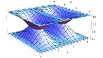
Figure 1: (Color online) The conditional entropy (upper surface) and the Euclidean distance (lower surface) of two steered states of the Alice’s qubit as a function of the Bob’s measurement parameters $(\theta,\phi)$ for a Bell-diagonal state with $(t_{1},t_{2},t_{3})=(-0.5,0.7,0.5)$. The figure shows that these functions have opposite behaviour under local measurement on the Bob’s qubit.

Motivated by the above observation, in what follows we are looking to those measurements on Bob’s qubit that cause the most disturbance in the Alice’s post-measurements states. To this aim we use the trace distance as a measure of quantum distinguishability between two outcomes NielsenBook2000

$$D(\rho^{A}_{0},\rho^{A}_{1})={\mathrm{Tr}}{|\rho^{A}_{0}-\rho^{A}_{1}|}.$$ (12)

This, in turns, reduces simply to the Euclidian distance $D(\widetilde{\boldsymbol{x}}_{0},\widetilde{\boldsymbol{x}}_{1})$ between Bloch vectors of the two post-measurement states $\rho_{0}^{A}$ and $\rho_{1}^{A}$. For the squared distance we find

$$D^{2}(\widetilde{\boldsymbol{x}}_{0},\widetilde{\boldsymbol{x}}_{1})=|\widetilde{\boldsymbol{x}}_{0}-\widetilde{\boldsymbol{x}}_{1}|^{2}=\frac{4\hat{\boldsymbol{n}}^{\mathrm{t}}M\hat{\boldsymbol{n}}}{(1-\hat{\boldsymbol{n}}^{\mathrm{t}}Y\hat{\boldsymbol{n}})^{2}},$$ (13)

where $Y=\boldsymbol{y}\boldsymbol{y}^{\mathrm{t}}$ and $M=m^{\mathrm{t}}m$ with $m=(T-\boldsymbol{x}\boldsymbol{y}^{\mathrm{t}})$. Maximum distinguishability corresponds therefore to the maximum distance given by

$$D^{2}_{\max}(\widetilde{\boldsymbol{x}}_{0},\widetilde{\boldsymbol{x}}_{1})=\max_{\hat{\boldsymbol{n}}}\left[\frac{4\hat{\boldsymbol{n}}^{\mathrm{t}}M\hat{\boldsymbol{n}}}{(1-\hat{\boldsymbol{n}}^{\mathrm{t}}Y\hat{\boldsymbol{n}})^{2}}\right],$$ (14)

where maximum is taken over all unit vectors $\hat{\boldsymbol{n}}\in\mathbb{R}^{3}$. Before we proceed further to find conditions under which $D^{2}(\widetilde{\boldsymbol{x}}_{0},\widetilde{\boldsymbol{x}}_{1})$ is maximize, let us turn our attention on some particular cases for which the maximum is obtained analytically without any need for rigorous optimization.
(i) Canonical states $\boldsymbol{y}=0$.—For the important class of canonical states for which the Bob’s coherence vector is zero, the optimum measurement leading to the maximum distance between Bloch vectors of the post-measurement states is nothing but the eigenvector of $T$ corresponding to its largest eigenvalue. Therefore in this case we have $D^{2}_{\max}(\widetilde{\boldsymbol{x}}_{0},\widetilde{\boldsymbol{x}}_{1})=4\max\{t_{1}^{2},t_{2}^{2},t_{3}^{2}\}$. The Bell-diagonal states, for which the Alice’s coherence vector also vanishes, are an important subclass of canonical states.
(ii) States for which $\boldsymbol{y}$ is an eigenvector corresponding to the largest eigenvalue of $M$.—In this case maximum of the enumerate happens in the direction of coherence vector of the part $B$, i.e. $\max_{\hat{\boldsymbol{n}}}\hat{\boldsymbol{n}}^{\mathrm{t}}M\hat{\boldsymbol{n}}=\boldsymbol{y}^{\mathrm{t}}M\boldsymbol{y}/y^{2}$. For such states we get $D^{2}_{\max}(\widetilde{\boldsymbol{x}}_{0},\widetilde{\boldsymbol{x}}_{1})=\left[\frac{4\boldsymbol{y}^{\mathrm{t}}M\boldsymbol{y}}{y^{2}(1-y^{2})^{2}}\right]$.
(iii) $X$ states.—The important class of $X$ states is defined by $\boldsymbol{x}=\left(\begin{array}[]{ccc}0&0&x\end{array}\right)^{\mathrm{t}}$, $\boldsymbol{y}=\left(\begin{array}[]{ccc}0&0&y\end{array}\right)^{\mathrm{t}}$, and $T={\mathrm{diag}}\{t_{1},t_{2},t_{3}\}$. In this case $M$ is also a diagonal matrix given by $M={\mathrm{diag}}\{M_{1},M_{2},M_{3}\}$ with $M_{1}=t_{1}^{2}$, $M_{2}=t_{2}^{2}$ and $M_{3}=(t_{3}-xy)^{2}$. In what follows we assume that $|t_{1}|\geq|t_{2}|$ ($|t_{1}|\leq|t_{2}|$ can be obtained just by replacing $1\rightarrow 2$ and $x\rightarrow y$). In this case we find the following results.

1. $M_{1}\leq M_{3}$. For such case we get $D_{\max}^{2}(\widetilde{\boldsymbol{x}}_{0},\widetilde{\boldsymbol{x}}_{1})=\frac{4M_{3}}{(1-y^{2})^{2}}$ with $\sigma_{z}$ as the optimal measurement.

2. $M_{1}\geq M_{3}$. In this case the optimal measurement is defined by $(\hat{n}^{\ast}_{1})^{2}=1-(\hat{n}^{\ast}_{3})^{2}$, $\hat{n}^{\ast}_{2}=0$, and $(\hat{n}^{\ast}_{3})^{2}=\frac{2M_{1}y^{2}-(M_{1}-M_{3})}{(M_{1}-M_{3})y^{2}}$ if

   $$\frac{M_{1}-M_{3}}{2M_{1}}\leq y^{2}\leq\frac{M_{1}-M_{3}}{M_{1}+M_{3}},$$ (15)

   or equivalently

   $$\left(\frac{2M_{3}}{M_{1}+M_{3}}\right)^{2}\leq(1-y^{2})^{2}\leq\left(\frac{M_{1}+M_{3}}{2M_{1}}\right)^{2}.$$ (16)

   On the other hand, the optimal measurement is $\sigma_{z}$, i.e. $D_{\max}^{2}(\widetilde{\boldsymbol{x}}_{0},\widetilde{\boldsymbol{x}}_{1})=\frac{4M_{3}}{(1-y^{2})^{2}}$, if

   $$\left(\frac{2M_{3}}{M_{1}+M_{3}}\right)^{2}\geq(1-y^{2})^{2},$$ (17)

   and it is $\sigma_{x}$, i.e. $D_{\max}^{2}(\widetilde{\boldsymbol{x}}_{0},\widetilde{\boldsymbol{x}}_{1})=4M_{1}$, if

   $$(1-y^{2})^{2}\geq\left(\frac{M_{1}+M_{3}}{2M_{1}}\right)^{2}.$$ (18)

Now, after giving the maximum distance for some particular classes of states without rigorous optimization, we provide in what follows an analytical procedure for optimization of Eq. (14). In order to determine the maximum distance, we have to calculate its derivatives with respect to $\theta$ and $\phi$. For derivative with respect to $\theta$ we get

$$\frac{\partial D^{2}}{\partial\theta}=\frac{8{\hat{\boldsymbol{n}}}_{,\theta}^{{\mathrm{t}}}\mathcal{M}({\hat{\boldsymbol{n}}}){\hat{\boldsymbol{n}}}}{(1-\hat{\boldsymbol{n}}^{\mathrm{t}}Y\hat{\boldsymbol{n}})^{2}},$$ (19)

where $\mathcal{M}({\hat{\boldsymbol{n}}})$ is a ${\hat{\boldsymbol{n}}}$-dependent symmetric matrix given by

$$\mathcal{M}({\hat{\boldsymbol{n}}})=M+\frac{2{\hat{\boldsymbol{n}}}^{\mathrm{t}}M{\hat{\boldsymbol{n}}}}{(1-\hat{\boldsymbol{n}}^{\mathrm{t}}Y\hat{\boldsymbol{n}})}Y,$$ (20)

and the unit vector ${\hat{\boldsymbol{n}}}_{,\theta}$ is defined by

$${\hat{\boldsymbol{n}}}_{,\theta}=\frac{\partial{\hat{\boldsymbol{n}}}}{\partial\theta}=(\cos{\theta}\cos{\phi},\cos{\theta}\sin{\phi},-\sin{\theta})^{{\mathrm{t}}}.$$ (21)

Evidently ${\hat{\boldsymbol{n}}}_{,\theta}\cdot{\hat{\boldsymbol{n}}}=0$. By defining the nonunit vector $\tilde{\boldsymbol{n}}_{,\phi}$ by

$${\tilde{\boldsymbol{n}}}_{,\phi}=\frac{\partial{\hat{\boldsymbol{n}}}}{\partial\phi}=(-\sin{\theta}\sin{\phi},\sin{\theta}\cos{\phi},0)^{{\mathrm{t}}},$$ (22)

orthogonal to both ${\hat{\boldsymbol{n}}}$ and ${\hat{\boldsymbol{n}}}_{,\theta}$, we get a similar equation for the derivative of the distance with respect to $\phi$, but now ${\hat{\boldsymbol{n}}}_{,\theta}$ is replaced by ${\tilde{\boldsymbol{n}}}_{,\phi}$. Excluding the case $y=1$ which happens if and only if the overall state is pure, we find the following relation for the stationary condition $\frac{\partial D^{2}}{\partial\theta}=\frac{\partial D^{2}}{\partial\phi}=0$,

$${\hat{\boldsymbol{n}}}_{\perp}^{{\mathrm{t}}}\;\mathcal{M}({\hat{\boldsymbol{n}}})\;{\hat{\boldsymbol{n}}}=0,$$ (23)

where $\hat{\boldsymbol{n}}_{\perp}$ is any vector perpendicular to $\hat{\boldsymbol{n}}$, i.e. $\hat{\boldsymbol{n}}_{\perp}\cdot\hat{\boldsymbol{n}}=0$. This implies that the stationary points are achieved if and only if ${\hat{\boldsymbol{n}}}$ be an eigenvector of $\mathcal{M}({\hat{\boldsymbol{n}}})$. Note that knowing the extremum points of the distance is not enough to establish its maximum, and we are required a further investigation of the distance over all extremum points to get the maximum one. Although condition (23) does not provide an easy solution for the maximum of the distance, due to the dependence of the symmetric matrix $\mathcal{M}({\hat{\boldsymbol{n}}})$ on the unknown direction ${\hat{\boldsymbol{n}}}$, it provides still a simple condition to evaluate the stationary points numerically. Not surprisingly, the above stationary condition is fulfilled for the special classes of states for which we have already obtained the maximum distance without rigorous optimization.

From the discussion given at the beginning of this section, two questions are being raised. The first one is that, is there any relation between the optimum measurement associated with the maximum distinguishability of the Alice’s outcomes with the one that allows one to extract the most information about the Alice’s qubit? We demonstrate in the following section that this is, indeed, the case. To do so, we provide some examples for which these two optimum measurements coincide exactly. The second question is that, when the optimum measurement of the maximum distinguished-outcomes process differs from the most information-gathering one, whether the former can be used to find a tight and faithful upper bound on the quantum discord? We will address these questions in the next section.

IV Maximum distinguished-outcomes measurement versus the most information-gathering one

Suppose Bob performs a measurement on his qubit in the direction $\hat{\boldsymbol{n}}^{\ast}$ which fulfills the maximum distinguishability condition (14). Using this in the definition of quantum discord we find that

$$Q_{B}(\rho)\leq Q_{B}^{\ast}(\rho),$$ (24)

where $Q_{B}(\rho)$ is the quantum discord of $\rho$, Eq. (2), and $Q_{B}^{\ast}(\rho)$ is its upper bound defined by

$${Q_{B}^{\ast}}({\rho}) = S({\rho^{B}})-S({\rho^{AB}})+S({\rho^{A}}|\,\{\Pi^{\ast B}_{k}\})$$ (25)

$$= [h_{2}(\vec{q})-h_{4}(\vec{\lambda})]+[h_{4}(\vec{w})-h_{2}(\vec{p})].$$

Above, $\Pi^{\ast B}_{k}=\frac{1}{2}\left({\mathbb{1}}+\hat{\boldsymbol{n}}^{\ast}_{k}\cdot\boldsymbol{\sigma}\right)$ for $k=0,1$ is the optimum measurement that maximizes $D^{2}(\widetilde{\boldsymbol{x}}_{0},\widetilde{\boldsymbol{x}}_{1})$. Moreover, $h_{m}(\vec{x})$ stands for the Shannon entropy of a probability vector of length $m$. Also $\vec{\lambda}$ and $\vec{q}$ denotes the probability vectors constructed from the eigenvalues of $\rho$ and $\rho^{B}$, respectively, and $\vec{w}$ and $\vec{p}$ are two probability vectors of length 4 and 2, respectively, given by AkhtarshenasIJTP2015

$$w_{k,l} = \frac{1}{4}\left\{{1+(-)^{k}\boldsymbol{y}\cdot\hat{\boldsymbol{n}}^{\ast}+(-)^{l}\left|\boldsymbol{x}+(-)^{k}T\hat{\boldsymbol{n}}^{\ast}\right|}\right\},$$ (26)

$$p_{k} = \frac{1}{2}\left\{1+(-)^{k}\boldsymbol{y}\cdot\hat{\boldsymbol{n}}^{\ast}\right\},$$ (27)

for $k,l\in\{0,1\}$. The following lemma shows that the above upper bound is faithful in a sense that it vanishes if and only if the bounded quantity vanishes.

Lemma 1.

$Q^{\ast}_{B}(\rho)=0$ if and only if $Q_{B}(\rho)=0$.

Proof.

The sufficient condition is a simple consequence of Eq. (24). To prove the necessary condition, let $\rho$ be a zero-discord on the Bob’s side. A two-qubit state has zero discord on Bob’s side if and only if either (i) $T=0$, or (ii) ${\mathrm{r}ank}(T)=1$ and $\boldsymbol{y}$ belongs to the range of $T$ LuPRA2011 ; Saman . We need therefore to prove that both cases lead to $Q_{B}^{\ast}(\rho)=0$.

(i) If $T=0$, we have from Eq. (14)

$$D^{2}_{\max}(\widetilde{\boldsymbol{x}}_{0},\widetilde{\boldsymbol{x}}_{1})=\max_{\hat{\boldsymbol{n}}}\left[\frac{4x^{2}(\hat{\boldsymbol{n}}\cdot\boldsymbol{y})^{2}}{(1-(\hat{\boldsymbol{n}}\cdot\boldsymbol{y})^{2})^{2}}\right],$$

which takes its maximum value for $\hat{\boldsymbol{n}}^{\ast}=\hat{\boldsymbol{y}}=\boldsymbol{y}/|\boldsymbol{y}|$. On the other hand, in this case, simple calculation shows that eigenvalues of $\rho$ and $\rho^{B}$ are given by

$$\lambda_{k,l} = \frac{1}{4}\left\{1+(-)^{k}y+(-)^{l}x\right\},\quad q_{k}=\frac{1}{2}\left\{1+(-)^{k}y\right\},$$

respectively ($k,l\in\{0,1\}$). Using these and putting $T=0$ in Eqs. (26) and (27), we find from Eq. (25) that $\hat{\boldsymbol{n}}^{\ast}=\hat{\boldsymbol{y}}$ gives ${Q_{B}^{\ast}}({\rho})=0$.

(ii) For the second case, i.e. when ${\mathrm{r}ank}(T)=1$ and $\boldsymbol{y}$ belongs to the range of $T$, without any loss of generality we assume that $\boldsymbol{y}$ and $T$ have the form $\boldsymbol{y}=y\hat{\boldsymbol{k}}$ and $T=t\hat{\boldsymbol{k}}\hat{\boldsymbol{k}}^{\mathrm{t}}$, respectively. In this case Eq. (14) leads to

$$D^{2}_{\max}(\widetilde{\boldsymbol{x}}_{0},\widetilde{\boldsymbol{x}}_{1})=\max_{\hat{\boldsymbol{n}}}\left[\frac{\left({{t}^{2}+{x^{2}}{\kern 1.0pt}{\kern 1.0pt}{y}^{2}-2{\kern 1.0pt}{\kern 1.0pt}{t}{\kern 1.0pt}{\kern 1.0pt}{x}{\kern 1.0pt}{\kern 1.0pt}{y}}\right)(\hat{\boldsymbol{n}}\cdot\hat{\boldsymbol{k}})^{2}}{(1-{y}^{4}(\hat{\boldsymbol{n}}\cdot\hat{\boldsymbol{k}})^{2})^{2}}\right],$$

which takes its maximum value for $\hat{\boldsymbol{n}}^{\ast}=\hat{\boldsymbol{k}}$. For such states we have

$$\lambda_{k,l} = \frac{1}{4}\left\{1+(-)^{k}y+(-)^{l}\left|\boldsymbol{x}+(-)^{k}T\hat{\boldsymbol{k}}\right|\right\},$$

$$q_{k} = \frac{1}{2}\left\{1+(-)^{k}y\right\},$$

for eigenvalues of $\rho$ and $\rho^{B}$, respectively. Moreover, $w_{k,l}$ and $p_{k}$ are given by Eqs. (26) and (27) with $\boldsymbol{y}=y\hat{\boldsymbol{k}}$ and $T=t\hat{\boldsymbol{k}}\hat{\boldsymbol{k}}^{\mathrm{t}}$. A simple investigation shows that ${Q_{B}^{\ast}}({\rho})=0$ for $\hat{\boldsymbol{n}}^{\ast}=\hat{\boldsymbol{k}}$. This completes the proof. ∎

In what follows we show that the above upper bound is tight in a sense that in more situations the equality is saturated. To this aim we consider states that we have considered in the last subsection.

(i) Canonical states $\boldsymbol{y}=0$.—There is no complete solution to the quantum discord of the canonical states, although their geometry and optimization formula are simpler than the general states. Without losing generality we assume $\left|{{t_{1}}}\right|\geq\left|{{t_{2}}}\right|$ and then do measurement along the greater semi-axis between $\hat{\boldsymbol{i}}$ and $\hat{\boldsymbol{k}}$. We do this and plot the results versus the quantum discord in Fig. 2 for more than 20000 random states. There are many points on the bisector line showing that the optimized direction is very near to the direction of our upper bound. Moreover, non-exact results are not too far from quantum discord and distribution of points near the bisector line shows that the upper bound is very near to the quantum discord. Canonical states with $T^{\mathrm{t}}\boldsymbol{x}=0$ have been solved analytically in AkhtarshenasIJTP2015 and it is easy to see that for this subclass we have $Q_{B}(\rho)=Q_{B}^{\ast}(\rho)$.

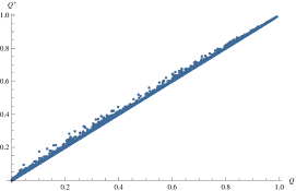
Figure 2: (Color online) The upper bound $Q^{\ast}(\rho)$ vs. quantum discord $Q(\rho)$ for 20000 random canonical states. Points on the bisector line belong to states for which the upper bound is equal to QD.

(ii) States for which $\boldsymbol{y}$ is an eigenvector corresponding to the largest eigenvalue of $M$.—In this case there are some classes of states for which there exist a good agreement between $Q_{B}(\rho)$ and $Q^{\ast}_{B}(\rho)$. Consider states with

$$\boldsymbol{x}=x\hat{\boldsymbol{k}},\qquad\boldsymbol{y}=y\hat{\boldsymbol{i}},\qquad T={\mathrm{diag}}\{{t_{1}},{t_{2}},0\}.$$ (28)

In this case $M={\mathrm{diag}}\{{t_{1}}^{2}+{x^{2}}{y^{2}},{t_{2}}^{2},0\}$, and when ${t_{1}}^{2}+{x^{2}}{y^{2}}\geq{t_{2}}^{2}$ both $Q_{B}(\rho)$ and $Q_{B}^{\ast}(\rho)$ are obtained by measurement along $\boldsymbol{y}$. In Fig. 3 we have plotted $Q_{B}^{\ast}(\rho)$ versus $Q_{B}(\rho)$ for more than 3000 random states of this category.

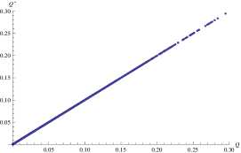
Figure 3: (Color online) The upper bound $Q^{\ast}(\rho)$ vs. quantum discord $Q(\rho)$ for 3000 random states for which $\boldsymbol{y}$ is an eigenvector corresponding to the largest eigenvalue of $M$. Results have high accuracy with $RE<10^{-6}$.

(iii) $X$ states.—For $X$-states we consider the following classes separately.

1. $M_{1}\leq M_{3}$. In this case $Q_{B}^{\ast}(\rho)$ is very near to $Q_{B}(\rho)$ and the relative error is less than $10^{-6}$. For 10000 random states of this category any point lies on the bisector line (Fig. 4).

   

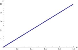
   Figure 4: (Color online) The upper bound $Q^{\ast}(\rho)$ vs. quantum discord $Q(\rho)$ for 10000 random $X$ states satisfying $M_{1}\leq M_{3}$. Results have high accuracy with $RE<10^{-6}$.

2. $M_{1}\geq M_{3}$. In Figs . 5 and 6 we plot $Q_{B}^{\ast}(\rho)$ vs. $Q_{B}(\rho)$ for 20000 random states satisfying one of the Eqs. (17) and (18), and 5000 random states satisfying Eq. (16), respectively.

Figure 5: (Color online) The upper bound $Q_{B}^{\ast}(\rho)$ vs. quantum discord $Q_{B}(\rho)$ for 20000 random $X$ states satisfying $M_{1}\geq M_{3}$ and one of the Eqs. (17) and (18).

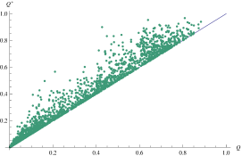
Figure 6: (Color online) The upper bound $Q_{B}^{\ast}(\rho)$ vs. quantum discord $Q_{B}(\rho)$ for 5000 random $X$ states satisfying $M_{1}\geq M_{3}$ and Eq. (16).

IV.1 $Q_{B}^{\ast}(\rho)$ as a tight upper bound

Now we proceed to employ $Q_{B}^{\ast}(\rho)$ as an upper bound and check if it is a tight one. Here we focus on a two parameters state as AlqasimiPRA2011

$$\rho=\frac{1}{2}\left({\begin{array}[]{*{20}{c}}a&0&0&a\\ 0&{1-a-b}&0&0\\ 0&0&{1-a+b}&0\\ a&0&0&a\end{array}}\right)\,,$$ (29)

where $0\leq a\leq 1$ and $a-1\leq b\leq 1-a$. The quantum discord of this state is AlqasimiPRA2011

$$Q_{B}(\rho)=\min\{a,q\},$$ (30)

where

$$q = \frac{a}{2}\,\log_{2}[\frac{{4\,{a^{2}}}}{{{{\left({1-a}\right)}^{2}}-{b^{2}}}}]-\frac{b}{2}\,log_{2}[\frac{{(1+b)(1-a-b)}}{{(1-b)(1-a+b)}}]$$

$$+ \frac{1}{2}\,\log_{2}[\frac{{4({{(1-a)}^{2}}-{b^{2}})}}{{(1-{b^{2}})(1-{a^{2}}-{b^{2}})}}]-\frac{{\sqrt{{a^{2}}+{b^{2}}}}}{2}\,\log_{2}[\frac{{1+\sqrt{{a^{2}}+{b^{2}}}}}{{1-\sqrt{{a^{2}}+{b^{2}}}}}].$$

Here $a$ and $q$ are obtained by measurements $\hat{\boldsymbol{n}}=\hat{\boldsymbol{i}}$ and $\hat{\boldsymbol{n}}=\hat{\boldsymbol{k}}$, respectively. Marginal coherence vectors and the correlation matrix of this state are given by

$$\boldsymbol{x}=-\boldsymbol{y}=\left({\begin{array}[]{c}0\\ 0\\ {-b}\end{array}}\right),\qquad T=\left({\begin{array}[]{ccc}a&0&0\\ 0&-a&0\\ 0&0&2a-1\end{array}}\right).$$ (32)

On the other hand, the maximal distance of this state is

$$D^{2}_{\max}=\max\left\{a^{2},\frac{{{{\left({(2a-1)+{b^{2}}}\right)}^{2}}}}{{{{\left({1-{b^{2}}}\right)}^{2}}}}\right\},$$ (33)

where $a^{2}$ and $\frac{{{{\left({(2a-1)+{b^{2}}}\right)}^{2}}}}{{{{\left({1-{b^{2}}}\right)}^{2}}}}$ are obtained by measurements $\hat{\boldsymbol{n}}=\hat{\boldsymbol{i}}$ and $\hat{\boldsymbol{n}}=\hat{\boldsymbol{k}}$, respectively.

Evidently, for $b=0$ we have $Q_{B}(\rho)=Q_{B}^{\ast}(\rho)$. In Fig. 7 we plot $Q_{B}(\rho)$ and $Q_{B}^{\ast}(\rho)$ as a function of $a$ for two cases $b=0.3$ and $b=0.7$, respectively. Except at a very small interval, we have $Q_{B}(\rho)=Q_{B}^{\ast}(\rho)$. A comparison of these figures reveals that as $b$ increases the amounts of QD decreases and also the interval in which $Q_{B}(\rho)\neq Q_{B}^{\ast}(\rho)$, grows up. Therefore, we observe that in high discordant states $Q_{B}^{\ast}(\rho)$ is more precise.

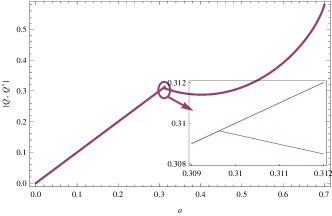
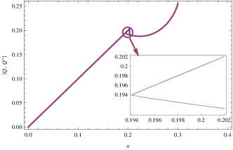
Figure 7: (Color online) $Q_{B}(\rho)$ and $Q_{B}^{\ast}(\rho)$ as a function of $a$ for (a) $b=0.3$ and (b) $b=0.7$. The insets show behaviour in the rigion near $Q_{B}(\rho)\neq Q_{B}^{\ast}(\rho)$.

V Conclusion

Here we have defined $Q^{\ast}(\rho)$ as the correlation that Bob can extract about Alice’s qubit by means of the most distinguishable measurements, i.e. measurements that Bob steers Alice to the most distinguishable states. For some classes of states, we have shown that this quantity is equal to the quantum discord $Q(\rho)$. Although $Q^{\ast}(\rho)$ may contain some classical correlations, the amount of classical correlations is not so much in particular for high discordant states. The presented quantity provides a faithful and tight upper bound for the quantum discord. Marginal states at high discordant states have high mixedness and so they are near to the Bell-diagonal states, for which $Q^{\ast}(\rho)$ coincides exactly with $Q(\rho)$.

The significance of our method comes from two facts: (i) the tightness of the provided bound and (ii) the physical interpretation of this bound. As we mentioned above, the provided upper bound is faithful and tight, meaning that the bound vanishes if and only if the bounded quantity vanishes. This, in turn, indicates that a nonzero value for the upper bound is a guarantee for the nonzero quantum discord, a fact that is not valid, in general, for an arbitrary upper bound. In other words, for zero discord states with possible classical correlations, the most distinguishable measurement washes out all classical correlations. On the other hand, the physical interpretation of our method is related to its relevance to the notion of quantum distinguishability. Actually a look at measure of distinguishability of two states, given by Eq. (12) for outcomes of the Alice’s side when Bob performs a von Neumann measurement on his particle, shows that this measure is closely related to the notion of minimum-error probability of discrimination of two states for equal a priori probability NielsenBook2000 .

The generalization of the above method is not straightforward as there are not well known geometries like Bloch sphere and quantum steering ellipsoid for arbitrary bipartite systems. For a general bipartite state with arbitrary dimension for Bob’s particle, when Bob performs POVM measurement on his particle with $n$ outcomes, the state of the Alice’s side steers to $\rho^{A}_{k}$ with probability $p_{k}$ corresponding to each outcome $k=1,\cdots,n$. Following the route of two-qubit system, we left therefore with the problem of finding the best possible measurement on the Bob’s side with the outputs that are most distinguishable on the Alice’s side. This, however, is not an easy task to treat in general and further study on the subject is under our investigation.

- (1) Schrödinger, E.: Discussion of probability relations between separated systems. Proc. Cambridge Philos. Soc. 31, 555-563 (1935).
- (2) Schrödinger, E.: Probability relations between separated systems Proc. Cambridge Philos. Soc. 32, 446-452 (1936).
- (3) Einstein, A., Podolsky, B., Rosen, N.: Can quantum-mechanical description of physical reality be considered complete?. Phys. Rev. 47, 777-780 (1935).
- (4) Milne, A., Jevtic, S., Pusey, M., Jennings, D., Rudolph, T.: Quantum steering ellipsoids. Phys. Rev. Lett. 113, 020402 (2014).
- (5) Milne, A., Jevtic, S., Jennings, D., Wiseman, H., Rudolph, T.: Quantum steering ellipsoids, extremal physical states and monogamy. New J. Phys. 16, 083017 (2014).
- (6) Milne, A., Jevtic, S., Jennings, D., Wiseman, H., Rudolph, T.: Corrigendum: quantum steering ellipsoids, extremal physical states and monogamy. New J. Phys. 17, 019501 (2015).
- (7) Milne, A., Jennings, D., Jevtic, S., Rudolph, T.: Quantum correlations of two-qubit states with one maximally mixed marginal. Phys. Rev. A 90, 024302 (2014).
- (8) Hu, X., Fan, H.: Effect of local channels on quantum steering ellipsoids. Phys. Rev. A 91, 022301 (2015).
- (9) Shi, M., Jiang, F., Sun, C., Du, J.: Geometric picture of quantum discord for two-qubit quantum states. New J. Phys. 13, 073016 (2011).
- (10) Wang, M., Gong, Q., Ficek, Z., He, Q.: Role of thermal noise in tripartite quantum steering. Phys. Rev. A 90, 023801 (2014).
- (11) McCloskey, R., Ferraro, A., Paterostro, M.: Einstein-Podolsky-Rosen steering and quantum steering ellipsoids: Optimal two-qubit states and projective measurements. Phys. Rev. A 95, 012320 (2017).
- (12) Jones, S.J., Wiseman, H.M., Doherty, A.C.: Entanglement, Einstein-Podolsky-Rosen correlations, Bell nonlocality, and steering. Phys. Rev. A 76, 052116 (2007).
- (13) Wiseman, H.M., Jones, S.J., Doherty, A.C.: Steering, entanglement, nonlocality, and the Einstein-Podolsky-Rosen paradox. Phys. Rev. Lett. 98, 140402 (2007).
- (14) Skrzypczyk, P., Navascués, M., Cavalcanti, D.: Quantifying Einstein-Podolsky-Rosen steering. Phys. Rev. Lett. 112, 180404 (2014).
- (15) Braun, D., Giraud, O., Nechita, I., Pellegrini, C., Znidaric, M.: A universal set of qubit quantum channels. J. Phys. A: Math. Theor. 47, 135302 (2014).
- (16) Peres, A.: Separability criterion for density matrices. Phys. Rev. Lett. 77, 1413-1415 (1996).
- (17) Horodecki, M., Horodecki, P., Horodecki, R.: Separability of mixed states: necessary and sufficient conditions. Phys. Lett. A 223, 1-8 (1996).
- (18) Ollivier, H., Zurek, W.H.: Quantum discord: A measure of the quantumness of correlations. Phys. Rev. Lett. 88, 017901 (2002).
- (19) Henderson, L. Vedral, V.: Classical, quantum and total correlations. J. Phys. A 34, 6899-6905 (2001).
- (20) Modi, K., Brodutch, A., Cable, H., Paterek, T., Vedral, V.: The classical-quantum boundary for correlations: Discord and related measures. Rev. Mod. Phys. 84, 1655-1707 (2012).
- (21) Girolami, D., Adesso, G.: Quantum discord for general states: Analytical progress. Phys. Rev. A 83, 052108 (2011).
- (22) Akhtarshenas, S.J., Mohammadi, H., Mousavi, F.S., Nassajpour, V.: Progress on quantum discord of two qubit states: Optimization and upper bound. Int. J. Theor. Phys. 54, 72-84 (2015).
- (23) Luo, S.: Quantum discord for two-qubit systems. Phys. Rev. A 77, 042303 (2008).
- (24) Lang, M.D., Caves, C.M.: Quantum discord and the geometry of Bell-diagonal states. Phys. Rev. Lett. 105, 150501 (2010).
- (25) Ali, M., Rau, A.R.P., Alber, G.: Quantum discord for two-qubit X states. Phys. Rev. A 81, 042105 (2010).
- (26) Chen, Q., Zhang, C., Yu, S., Yi, X.X., Oh, C.H.: Quantum discord of two-qubit X states. Phys. Rev. A 84, 042313 (2011).
- (27) Shi, M., Yang, W., Jiang, F., Du, J.: Quantum discord of two-qubit rank-2 states. J. Phys. A: Math. Theor. 44, 415304 (2011).
- (28) Wu, X., Zhou, T.: Quantum discord for the general two-qubit case. Quantum Inf. Process. 14, 1959-1971 (2015).
- (29) Verstraete, F., Dehaene, J., DeMoor, B.: Local filtering operations on two qubits. Phys. Rev. A 64, 010101 (2001).
- (30) Nielsen, M.A., Chuang, I.L.: Quantum computation and quantum information. (Cambridge University Press, Cambridge, UK 2000).
- (31) Lu, X-M, Ma, J., Xi, Z., Wang, X.: Optimal measurements to access classical correlations of two-qubit states. Phys. Rev. A 83, 012327 (2011).
- (32) Akhtarshenas, S.J., Mohammadi, H., Karimi, S., Azmi, Z.: Computable measure of quantum correlation. Quantum Inf. Process., 14, 247-267 (2015).
- (33) Al-Qasimi, A., Jams, D.F.V.: Comparison of the attempts of quantum discord and quantum entanglement to capture quantum correlations. Phys. Rev. A 83, 032101 (2011).