Evaluating Design Tradeoffs in Numeric Static Analysis for Java

Abstract

Numeric static analysis for Java has a broad range of potentially useful applications, including array bounds checking and resource usage estimation. However, designing a scalable numeric static analysis for real-world Java programs presents a multitude of design choices, each of which may interact with others. For example, an analysis could handle method calls via either a top-down or bottom-up interprocedural analysis. Moreover, this choice could interact with how we choose to represent aliasing in the heap and/or whether we use a relational numeric domain, e.g., convex polyhedra. In this paper, we present a family of abstract interpretation-based numeric static analyses for Java and systematically evaluate the impact of 162 analysis configurations on the DaCapo benchmark suite. Our experiment considered the precision and performance of the analyses for discharging array bounds checks. We found that top-down analysis is generally a better choice than bottom-up analysis, and that using access paths to describe heap objects is better than using summary objects corresponding to points-to analysis locations. Moreover, these two choices are the most significant, while choices about the numeric domain, representation of abstract objects, and context-sensitivity make much less difference to the precision/performance tradeoff.

1 Introduction

Static analysis of numeric program properties has a broad range of useful applications. Such analyses can potentially detect array bounds errors [53], analyze a program’s resource usage [30, 28], detect side channels [11, 8], and discover vectors for denial of service attacks [10, 26].

One of the major approaches to numeric static analysis is abstract interpretation [18], in which program statements are evaluated over an abstract domain until a fixed point is reached. Indeed, the first paper on abstract interpretation [18] used numeric intervals as one example abstract domain, and many subsequent researchers have explored abstract interpretation-based numeric static analysis [25, 23, 24, 22, 13, 31].

Despite this long history, applying abstract interpretation to real-world Java programs remains a challenge. Such programs are large, have many interacting methods, and make heavy use of heap-allocated objects. In considering how to build an analysis that aims to be sound but also precise, prior work has explored some of these challenges, but not all of them together. For example, several works have considered the impact of the choice of numeric domain (e.g., intervals vs. convex polyhedra) in trading off precision for performance but not considered other tradeoffs [24, 38]. Other works have considered how to integrate a numeric domain with analysis of the heap, but unsoundly model method calls [25] and/or focus on very precise properties that do not scale beyond small programs [23, 24]. Some scalability can be recovered by using programmer-specified pre- and post-conditions [22]. In all of these cases, there is a lack of consideration of the broader design space in which many implementation choices interact. (Section 7 considers prior work in detail.)

In this paper, we describe and then systematically explore a large design space of fully automated, abstract interpretation-based numeric static analyses for Java. Each analysis is identified by a choice of five configurable options—the numeric domain, the heap abstraction, the object representation, the interprocedural analysis order, and the level of context sensitivity. In total, we study 162 analysis configurations to asses both how individual configuration options perform overall and to study interactions between different options. To our knowledge, our basic analysis is one of the few fully automated numeric static analyses for Java, and we do not know of any prior work that has studied such a large static analysis design space.

We selected analysis configuration options that are well-known in the static analysis literature and that are key choices in designing a Java static analysis. For the numeric domain, we considered both intervals [17] and convex polyhedra [19], as these are popular and bookend the precision/performance spectrum. (See Section 2.)

Modeling the flow of data through the heap requires handling pointers and aliasing. We consider three different choices of heap abstraction: using summary objects [25, 27], which are weakly updated, to summarize multiple heap locations; access paths [21, 54], which are strongly updated; and a combination of the two.

To implement these abstractions, we use an ahead-of-time, global points-to analysis [47], which maps static/local variables and heap-allocated fields to abstract objects. We explore three variants of abstract object representation: the standard allocation-site abstraction (the most precise) in which each syntactic new in the program represents an abstract object; class-based abstraction (the least precise) in which each class represents all instances of that class; and a smushed string abstraction (intermediate precision) which is the same as allocation-site abstraction except strings are modeled using a class-based abstraction [9]. (See Section 3.)

We compare three choices in the interprocedural analysis order we use to model method calls: top-down analysis, which starts with main and analyzes callees as they are encountered; and bottom-up analysis, which starts at the leaves of the call tree and instantiates method summaries at call sites; and a hybrid analysis that is bottom-up for library methods and top-down for application code. In general, top-down analysis explores fewer methods, but it may analyze callees multiple times. Bottom-up analysis explores each method once but needs to create summaries, which can be expensive.

Finally, we compare three kinds of context-sensitivity in the points-to analysis: context-insensitive analysis, 1-CFA analysis [49] in which one level of calling context is used to discriminate pointers, and type-sensitive analysis [52] in which the type of the receiver is the context. (See Section 4.)

We implemented our analysis using WALA [2] for its intermediate representation and points-to analyses and either APRON [41, 33] or ELINA [50, 51] for the interval or polyhedral, respectively, numeric domain. We then applied all 162 analysis configurations to the DaCapo benchmark suite [6], using the numeric analysis to try to prove array accesses are within bounds. We measured the analyses’ performance and the number of array bounds checks they discharged. We analyzed our results by using a multiple linear regression over analysis features and outcomes, and by performing data visualizations.

We studied three research questions. First, we examined how analysis configuration affects performance. We found that using summary objects causes significant slowdowns, e.g., the vast majority of the analysis runs that timed out used summary objects. We also found that polyhedral analysis incurs a significant slowdown, but only half as much as summary objects. Surprisingly, bottom-up analysis provided little performance advantage generally, though it did provide some benefit for particular object representations. Finally, context-insensitive analysis is faster than context-sensitive analysis, as might be expected, but the difference is not great when combined with more approximate (class-based and smushed string) abstract object representations.

Second, we examined how analysis configuration affects precision. We found that using access paths is critical to precision. We also found that the bottom-up analysis has worse precision than top-down analysis, especially when using summary objects, and that using a more precise abstract object representation improves precision. But other traditional ways of improving precision do so only slightly (the polyhedral domain) or not significantly (context-sensitivity).

Finally, we looked at the precision/performance tradeoff for all programs. We found that using access paths is always a good idea, both for precision and performance, and top-down analysis works better than bottom-up. While summary objects, originally proposed by Fu [25], do help precision for some programs, the benefits are often marginal when considered as a percentage of all checks, so they tend not to outweigh their large performance disadvantage. Lastly, we found that the precision gains for more precise object representations and polyhedra are modest, and performance costs can be magnified by other analysis features.

In summary, our empirical study provides a large, comprehensive evaluation of the effects of important numeric static analysis design choices on performance, precision, and their tradeoff; it is the first of its kind. We plan to release our code and data to support further research and evaluation.

2 Numeric Static Analysis

Config. Option	Setting	Description
Numeric domain (ND)	INT	Intervals
	POL	Polyhedra
Heap abstraction (HA)	SO	Only summary objects
	AP	Only access paths
	AP+SO	Both access paths and summary objects
Abstract object representation (OR)	ALLO	Alloc-site abstraction
	CLAS	Class-based abstraction
	SMUS	Alloc-site except Strings
Inter-procedural analysis order (AO)	TD	Top-down
	BU	Bottom-up
	TD+BU	Hybrid top-down and bottom-up
Context sensitivity (CS)	CI	Context-insensitive
	1CFA	1-CFA
	1TYP	Type-sensitive

Table 1: Analysis configuration options, and their possible settings.

A numeric static analysis is one that tracks numeric properties of memory locations, e.g., that $x\leq 5$ or $y>z$. A natural starting point for a numeric static analysis for Java programs is numeric abstract interpretation over program variables within a single procedure/method [18].

A standard abstract interpretation expresses numeric properties using a numeric abstract domain, of which the most common are intervals (also known as boxes) and convex polyhedra. Intervals [17] define abstract states using inequalities of the form $p~{}\mathit{relop}~{}n$ where $p$ is a variable, $n$ is a constant integer, and $\mathit{relop}$ is a relational operator such as $\leq$. A variable such as $p$ is sometimes called a dimension, as it describes one axis of a numeric space. Convex polyhedra [19] define abstract states using linear relationships between variables and constants, e.g., of the form $3p_{1}-p_{2}\leq 5$. Intervals are less precise but more efficient than polyhedra. Operation on intervals have time complexity linear in the number of dimensions whereas the time complexity for polyhedra operations is exponential in the number of dimensions.

Numeric abstract interpretation, including our own analyses, are usually flow-sensitive, i.e., each program point has an associated abstract state characterizing properties that hold at that point. Variable assignments are strong updates, meaning information about the variable is replaced by information from the right-hand side of the assignment. At merge points (e.g., after the completion of a conditional), the abstract states of the possible prior states are joined to yield properties that hold regardless of the branch taken. Loop bodies are reanalyzed until their constituent statements’ abstract states reach a fixed point. Reaching a fixed point is accelerated by applying the numeric domain’s standard widening operator [4] in place of join after a fixed number of iterations.

Scaling a basic numeric abstract interpreter to full Java requires making many design choices. Table 1 summarizes the key choices we study in this paper. Each configuration option has a range of settings that potentially offer different precision/performance tradeoffs. Different options may interact with each other to affect the tradeoff. In total, we study five options with two or three settings each. We have already discussed the first option, the numeric domain (ND), for which we consider intervals (INT) and polyhedra (POL). The next two options consider the heap, and are discussed in the next section, and the last two options consider method calls, and are discussed in Section 4.

For space reasons, the main presentation focuses on the high-level design and tradeoffs. Detailed algorithms are given formally in Appendices 0.A and 0.B for the heap and interprocedural analysis, respectively.

3 The Heap

The numeric analysis described so far is sufficient only for analyzing code with local, numeric variables. To analyze numeric properties of heap-manipulating programs, we must also consider heap locations $x.f$, where $x$ is a reference to a heap-allocated object, and $f$ is a numeric field. To do so requires developing a heap abstraction (HA) that accounts for aliasing. In particular, when variables $x$ and $y$ may point to the same heap object, an assignment to $x.f$ could affect $y.f$. Moreover, the referent of a pointer may be uncertain, e.g., the true branch of a conditional could assign location $o_{1}$ to $x$, while the false branch could assign $o_{2}$ to $x$. This uncertainty must be reflected in subsequent reads of $x.f$.

We use a points-to analysis to reason about aliasing. A points-to analysis computes a mapping $\mathit{Pt}$ from variables $x$ and access paths $x.f$ to (one or more) abstract objects [47]. If $\mathit{Pt}$ maps two variables/paths $p_{1}$ and $p_{2}$ to a common abstract object $o$ then $p_{1}$ and $p_{2}$ may alias. We also use points-to analysis to determine the call graph, i.e., to determine what method may be called by an expression $x.m(\ldots)$ (discussed in Section 4).

3.1 Summary objects (SO)

The first heap abstraction we study is based on Fu [25]: use a summary object (SO) to abstract information about multiple heap locations as a single abstract state “variable” [27]. As an example, suppose that $\mathit{Pt}(x)=\{o\}$ and we encounter the assignment $x.f\;\texttt{:=}\;5$. Then in this approach, we add a variable $o\_f$ to the abstract state, modeling the field $f$ of object $o$, and we add constraint $o\_f=n$. Subsequent assignments to such summary objects must be weak updates, to respect the may alias semantics of the points-to analysis. For example, suppose $y.f$ may alias $x.f$, i.e., $o\in\mathit{Pt}(x)\cap\mathit{Pt}(y)$. Then after a later assignment $y.f\;\texttt{:=}\;7$ the analysis would weakly update $o\_f$ with 7, producing constraints $5\leq o\_f\leq 7$ in the abstract state. These constraints conservatively model that either $o\_f=5$ or $o\_f=7$, since the assignment to $y.f$ may or may not affect $x.f$.

In general, weak updates are more expensive than strong updates, and reading a summary object is more expensive than reading a variable. A strong update to $x$ is implemented by forgetting $x$ in the abstract state, and then re-adding it to be equal to the assigned-to value. Note that $x$ cannot appear in the assigned-to value because programs are converted into static single assignment form (Section 5). A weak update—which is not directly supported in the numeric domain libraries we use—is implemented by copying the abstract state, strongly updating $x$ in the copy, and then joining the two abstract states. Reading from a summary object requires “expanding” the abstract state with a copy $o^{\prime}\_f$ of the summary object and its constraints, creating a constraint on $o^{\prime}\_f$, and then forgetting $o^{\prime}\_f$. Doing this ensures that operations on a variable into which a summary object is read do not affect prior reads. A normal read just references the read variable.

Fu [25] argues that this basic approach is better than ignoring heap locations entirely by measuring how often field reads are not unconstrained, as would be the case for a heap-unaware analysis. However, it is unclear whether the approach is sufficiently precise for applications such as array-bounds check elimination. Using the polyhedra numeric domain should help. For example, a Buffer class might store an array in one field and a conservative bound on an array’s length in another. The polyhedral domain will permit relating the latter to the former while the interval domain will not. But the slowdown due to the many added summary objects may be prohibitive.

3.2 Access paths (AP)

An alternative heap abstraction we study is to treat access paths (AP) as if they are normal variables, while still accounting for possible aliasing [21, 54]. In particular, a path $x.f$ is modeled as a variable $x\_f$, and an assignment $x.f\;\texttt{:=}\;n$ strongly updates $x\_f$ to be $n$. At the same time, if there exists another path $y.f$ and $x$ and $y$ may alias, then we must weakly update $y\_f$ as possibly containing $n$. In general, determining which paths must be weakly updated depends on the abstract object representation and context-sensitivity of the points-to analysis.

Two key benefits of AP over SO are that (1) AP supports strong updates to paths $x.f$, which are more precise and less expensive than weak updates, and (2) AP may require fewer variables to be tracked, since, in our design, access paths are mostly local to a method whereas points-to sets are computed across the entire program. On the other hand, SO can do better at summarizing invariants about heap locations pointed to by other heap locations, i.e., not necessarily via an access path. Especially when performing an interprocedural analysis, such information can add useful precision.

3.2.1 Combined (AP+SO)

A natural third choice is to combine AP and SO. Doing so sums both the costs and benefits of the two approaches. An assignment $x.f\;\texttt{:=}\;n$ strongly updates $x\_f$ and weakly updates $o\_f$ for each $o$ in $\mathit{Pt}(x)$ and each $y\_f$ where $\mathit{Pt}(x)\cap\mathit{Pt}(y)\neq\emptyset$. Reading from $x.f$ when it has not been previously assigned to is just a normal read, after first strongly updating $x\_f$ to be the join of the summary read of $o\_f$ for each $o\in\mathit{Pt}(x)$.

3.3 Abstract object representation (OR)

Another key precision/performance tradeoff is the abstract object representation (OR) used by the points-to analysis. In particular, when $Pt(x)=\{o_{1},...,o_{n}\}$, where do the names $o_{1},...,o_{n}$ come from? The answer impacts the naming of summary objects, the granularity of alias checks for assignments to access paths, and the precision of the call-graph, which requires aliasing information to determine which methods are targeted by a dynamic dispatch $x.m(...)$.

As shown in the third row of Table 1, we explore three representations for abstract objects. The first choice names abstract objects according to their allocation site (ALLO)—all objects allocated at the same program point have the same name. This is precise but potentially expensive, since there are many possible allocation sites, and each path $x.f$ could be mapped to many abstract objects. We also consider representing abstract objects using class names (CLAS), where all objects of the same class share the same abstract name, and a hybrid smushed string (SMUS) approach, where every String object has the same abstract name but objects of other types have allocation-site names [9]. The class name approach is the least precise but potentially more efficient since there are fewer names to consider. The smushed string analysis is somewhere in between. The question is whether the reduction in names helps performance enough, without overly compromising precision.

4 Method Calls

So far we have considered the first three options of Table 1, which handle integer variables and the heap. This section considers the last two options—interprocedural analysis order (AO) and context sensitivity (CS).

4.1 Interprocedural analysis order (AO)

We implement three styles of interprocedural analysis: top-down (TD), bottom-up (BU), and their combination (TD+BU). The TD analysis starts at the program entry point and, as it encounters method calls, analyzes the body of the callee (memoizing duplicate calls). The BU analysis starts at the leaves of the call graph and analyzes each method in isolation, producing a summary of its behavior [55, 29]. (We discuss call graph construction in the next subsection.) This summary is then instantiated at each method call. The hybrid analysis works top-down for application code but bottom-up for any code from the Java standard library.

4.1.1 Top-down (TD).

Assuming the analyzer knows the method being called, a simple approach to top-down analysis would be to transfer the caller’s state to the beginning of callee, analyze the callee in that state, and then transfer the state at the end of the callee back to the caller. Unfortunately, this approach is prohibitively expensive because the abstract state would accumulate all local variables and access paths across all methods along the call-chain.

We avoid this blowup by analyzing a call to method $m$ while considering only relevant local variables and heap abstractions. Ignoring the heap for the moment, the basic approach is as follows. First, we make a copy $C_{m}$ of the caller’s abstract state $C$. In $C_{m}$, we set variables for $m$’s formal numeric arguments to the actual arguments and then forget (as defined in Section 3.1) the caller’s local variables. Thus $C_{m}$ will only contain the portion of $C$ relevant to $m$. We analyze $m$’s body, starting in $C_{m}$, to yield the final state $C^{\prime}_{m}$. Lastly, we merge $C$ and $C^{\prime}_{m}$, strongly update the variable that receives the returned result, and forget the callee’s local variables—thus avoiding adding the callee’s locals to the caller’s state.

Now consider the heap. If we are using summary objects, when we copy $C$ to $C_{m}$ we do not forget those objects that might be used by $m$ (according to the points-to analysis). As $m$ is analyzed, the summary objects will be weakly updated, ultimately yielding state $C^{\prime}_{m}$ at $m$’s return. To merge $C^{\prime}_{m}$ with $C$, we first forget the summary objects in $C$ not forgotten in $C_{m}$ and then concatenate $C^{\prime}_{m}$ with $C$. The result is that updated summary objects from $C^{\prime}_{m}$ replace those that were in the original $C$.

If we are using access paths, then at the call we forget access paths in $C$ because assignments in $m$’s code might invalidate them. But if we have an access path $x.f$ in the caller and we pass $x$ to $m$, then we retain $x.f$ in the callee but rename it to use $m^{\prime}$s parameter’s name. For example, $x.f$ becomes $y.f$ if $m$’s parameter is $y$. If $y$ is never assigned to in $m$, we can map $y.f$ back to $x.f$ (in the caller) once $m$ returns. All other access paths in $C_{m}$ are forgotten prior to concatenating with the caller’s state.

Note that the above reasoning is only for numeric values. We take no particular steps for pointer values as the points-to analysis already tracks those across all methods.

4.1.2 Bottom up (BU).

In the BU analysis, we analyze a method $m$’s body to produce a method summary and then instantiate the summary at calls to $m$. Ignoring the heap, producing a method summary for $m$ is straightforward: start analyzing $m$ in a state $C_{m}$ in which its (numeric) parameters are unconstrained variables. When $m$ returns, forget all variables in the final state except the parameters and return value, yielding a state $C^{\prime}_{m}$ that is the method summary. Then, when $m$ is called, we concatenate $C^{\prime}_{m}$ with the current abstract state; add constraints between the parameters and their actual arguments; strongly update the variable receiving the result with the summary’s returned value; and then forget those variables.

When using the polyhedral numeric domain, $C^{\prime}_{m}$ can express relationships between input and output parameters, e.g., ret $\leq$ z or ret = x+y. For the interval domain, which is non-relational, summaries are more limited, e.g., they can express ret $\leq 100$ but not ret $\leq$ x. As such, we expect bottom-up analysis to be far more useful with the polyhedral domain than the interval domain.

Summary objects.

Now consider the heap. Recall that when using summary objects in the TD analysis, reading a path $x.f$ into $z$ “expands” each summary object $o\_f$ when $o\in Pt(x)$ and strongly updates $z$ with the join of these expanded objects, before forgetting them. This expansion makes a copy of each summary object’s constraints so that later use of $z$ does not incorrectly impact the summary. However, when analyzing a method bottom-up, we may not yet know all of a summary object’s constraints. For example, if $x$ is passed into the current method, we will not (yet) know if $o\_f$ is assigned to a particular numeric range in the caller.

We solve this problem by allocating a fresh, unconstrained placeholder object at each read of $x.f$ and include it in the initialization of the assigned-to variable $z$. The placeholder is also retained in $m$’s method summary. Then at a call to $m$, we instantiate each placeholder with the constraints in the caller involving the placeholder’s summary location. We also create a fresh placeholder in the caller and weakly update it to the placeholder in the callee; doing so allows for further constraints to be added from calls further up the call chain.

Access paths.

If we are using access paths, we treat them just as in TD—each $x.f$ is allocated a special variable that is strongly updated when possible, according to the points-to analysis. These are not kept in method summaries. When also using summary objects, at the first read to $x.f$ we initialize it from the summary objects derived from $x$’s points-to set, following the above expansion procedure. Otherwise $x.f$ will be unconstrained.

4.1.3 Hybrid (TD+BU).

In addition to TD or BU analysis (only), we implemented a hybrid strategy that performs TD analysis for the application, but BU analysis for code from the Java standard library. Library methods are analyzed first, bottom-up. Application method calls are analyzed top-down. When an application method calls a library method, it applies the BU method call approach. TD+BU could potentially be better than TD because library methods, which are likely called many times, only need to be analyzed once. TD+BU could similarly be better than BU because application methods, which are likely not called as many times as library methods, can use the lower-overhead TD analysis.

Now, consider the interaction between the heap abstraction and the analysis order. The use of access paths (only) does not greatly affect the normal TD/BU tradeoff: TD may yield greater precision by adding constraints from the caller when analyzing the callee, while BU’s lower precision comes with the benefit of analyzing method bodies less often. Use of summary objects complicates this tradeoff. In the TD analysis, the use of summary objects adds a relatively stable overhead to all methods, since they are included in every method’s abstract state. For the BU analysis, methods further down in the call chain will see fewer summary objects used, and method bodies may end up being analyzed less often than in the TD case. On the other hand, placeholder objects add more dimensions overall (one per read) and more work at call sites (to instantiate them). But, instantiating a summary may be cheaper than reanalyzing the method.

4.2 Context sensitivity (CS)

The last design choice we considered was context-sensitivity. A context-insensitive (CI) analysis conflates information from different call sites of the same method. For example, two calls to method $m$ in which the first passes $x_{1},y_{1}$ and the second passes $x_{2},y_{2}$ will be conflated such that within $m$ we will only know that either $x_{1}$ or $x_{2}$ is the first parameter, and either $y_{1}$ or $y_{2}$ is the second; we will miss the correlation between parameters. A context sensitive analysis provides some distinction among different call sites. A 1-CFA analysis [49] (1CFA) distinguishes based on one level of calling context, i.e., two calls originating from different program points will be distinguished, but two calls from the same point, but in a method called from two different points will not. A type-sensitive analysis [52] (1TYP) uses the type of the receiver as the context.

Context sensitivity in the points-to analysis affects alias checks, e.g., when determining whether an assignment to $x.f$ might affect $y.f$. It also affects the abstract object representation and call graph construction. Due to the latter, context sensitivity also affects our interprocedural numeric analysis. In a context-sensitive analysis, a single method is essentially treated as a family of methods indexed by a calling context. In particular, our analysis keeps track of the current context as a frame, and when considering a call to method x.m(), the target methods to which m may refer differ depending on the frame. This provides more precision than a context-insensitive (i.e., frame-less) approach, but the analysis may consider the same method code many times, which adds greater precision but also greater expense. This is true both for TD and BU, but is perhaps more detrimental to the latter since it reduces potential method summary reuse. On the other hand, more precise analysis may reduce unnecessary work by pruning infeasible call graph edges. For example, when a call might dynamically dispatch to several different methods, the analysis must consider them all, joining their abstract states. A more precise analysis may consider fewer target methods.

5 Implementation

We have implemented an analysis for Java with all of the options described in the previous two sections. Our implementation is based on the intermediate representation in the T. J. Watson Libraries for Analysis (WALA) version 1.3.10 [2], which converts a Java bytecode program into static single assignment (SSA) form [20], which is then analyzed. We use APRON [41, 33] trunk revision 1096 (published on 2016/05/31) implementation of intervals, and ELINA [50, 51], snapshot as of October 4, 2017, for convex polyhedra. Our current implementation supports all non-floating point numeric Java values and comprises 14K lines of Scala code.

Next we discuss a few additional implementation details.

Preallocating dimensions.

In both APRON and ELINA, it is very expensive to perform join operations that combine abstract states with different variables. Thus, rather than add dimensions as they arise during abstract interpretation, we instead preallocate all necessary dimensions—including for local variables, access paths, and summary objects, when enabled—at the start of a method body. This ensures the abstract states have the same dimensions at each join point. We found that, even though this approach makes some states larger than they need to be, the overall performance savings is still substantial.

Arrays.

Our analysis encodes an array as an object with two fields, contents, which represents the contents of the array, and len, representing the array’s length. Each read/write from a[i] is modeled as a weak read/write of contents (because all array elements are represented with the same field), with an added check that i is between $0$ and len. We treat Strings as a special kind of array.

Widening.

As is standard in abstract interpretation, our implementation performs widening to ensure termination when analyzing loops. In a pilot study, we compared widening after between one and ten iterations. We found that there was little added precision when applying widening after more than three iterations when trying to prove array indexes in bounds (our target application, discussed next). Thus we widen at that point in our implementation.

Limitations.

Our implementation is sound with a few exceptions. In particular, it ignores calls to native methods and uses of reflection. It is also unsound in its handling of recursive method calls. If the return value of a recursive method is numeric, it is regarded as unconstrained. Potential side effects of the the recursive calls are not modeled.

6 Evaluation

In this section, we present an empirical study of our family of analyses, focusing on the following research questions:

RQ1: Performance. How does the configuration affect analysis running time?

RQ2: Precision. How does the configuration affect analysis precision?

RQ3: Tradeoffs. How does the configuration affect precision and performance?

To answer these questions, we chose an important analysis client, array index out-of-bound analysis, and ran it on the DaCapo benchmark suite  [6]. We vary each of the analysis features listed in Table 1, yielding 162 total configurations. To understand the impact of analysis features, we used multiple linear regression and logistic regression to model precision and performance (the dependent variables) in terms of analysis features and across programs (the independent variables). We also studied per-program data directly.

Overall, we found that using access paths is a significant boon to precision but costs little in performance, while using summary objects is the reverse, to the point that use of summary objects is a significant source of timeouts. Polyhedra add precision compared to intervals, and impose some performance cost, though only half as much as summary objects. Interestingly, when both summary objects and polyhedra together would result in a timeout, choosing the first tends to provide better precision over the second. Finally, bottom-up analysis harms precision compared to top-down analysis, especially when only summary objects are enabled, but yields little gain in performance.

6.1 Experimental setup

We evaluated our analyses by using them to perform array index out of bounds analysis. More specifically, for each benchmark program, we counted how many array access instructions (x[i]=y, y=x[i], etc.) an analysis configuration could verify were in bounds (i.e., i<x.length), and measured the time taken to perform the analysis.

		#	Best Performance			Best Precision
Prog	Size	Checks	Time(min)	# Checks	Percent	Time(min)	# Checks	Percent
			BU-AP-CI-CLAS-INT			TD-AP+SO-1TYP-CLAS-INT
antlr	55734	1526	0.6	1176	77.1%	18.5	1306	85.6%
			BU-AP-CI-CLAS-INT			TD-AP-1TYP-SMUS-POL
bloat	150197	4621	4.0	2538	54.9%	17.2	2795	60.5%
			BU-AP-CI-CLAS-INT			TD-AP-1TYP-SMUS-INT
chart	167621	7965	3.3	5593	70.2%	7.7	5654	71.0%
			BU-AP-CI-ALLO-INT			TD-AP+SO-1TYP-SMUS-POL
eclipse	18938	1043	0.2	896	85.9%	3.3	977	93.7%
			BU-AP-CI-CLAS-INT			TD-AP+SO-1CFA-SMUS-INT
fop	33243	1337	0.4	998	74.6%	2.6	1137	85.0%
			BU-AP-CI-SMUS-INT			TD-AP+SO-CI-SMUS-INT
hsqldb	19497	1020	0.3	911	89.3%	1.4	975	95.6%
			BU-AP-CI-SMUS-INT			TD-AP-1CFA-CLAS-POL
jython	127661	4232	1.3	2667	63.0%	33.6	2919	69.0%
			BU-AP-CI-SMUS-INT			TD-AP+SO-1TYP-ALLO-INT
luindex	69027	2764	1.8	1682	60.9%	46.8	2015	72.9%
			BU-AP-CI-CLAS-INT			TD-AP+SO-1CFA-ALLO-POL
lusearch	20242	1062	0.2	912	85.9%	54.2	979	92.2%
			BU-AP-CI-CLAS-INT			TD-AP+SO-CI-CLAS-INT
pmd	116422	4402	1.7	3153	71.6%	49.5	3301	75.0%
			BU-AP-CI-CLAS-INT			TD-AP+SO-1CFA-SMUS-POL
xalan	20315	1043	0.2	912	87.4%	3.8	981	94.1%

Table 2: Benchmarks and overall results.

Benchmarks.

We analyzed all eleven programs from the DaCapo benchmark suite [6] version 2006-10-MR2. The first three columns of Table 2 list the programs’ names, their size (number of IR instructions), and the number of array bounds checks they contain. The rest of the table indicates the fastest and most precise analysis configuration for each program; we discuss these results in Section 6.4. We ran each benchmark three times under each of the 162 analysis configurations. The experiments were performed on two 2.4 GHz single processor (with four logical cores) Intel Xeon E5-2609 servers, each with 128GB memory running Ubuntu 16.04 (LTS). On each server, we ran three analysis configurations in parallel, binding each process to a designated core.

Since many analysis configurations are time-intensive, we set a limit of 1 hour for running a benchmark under a particular configuration. All performance results reported are the median of the three runs. We also use the median precision result, though note the analyses are deterministic, so the precision does not vary except in the case of timeouts. Thus, we treat an analysis as not timing out as long as either two or three of the three runs completed, and otherwise it is a timeout. Among the 1782 median results (11 benchmarks, 162 configurations), 667 of them (37%) timed out. The percentage of the configurations that timed out analyzing a program ranged from 0% (xalan) to 90% (chart).

Statistical Analysis.

To answer RQ1 and RQ2, we constructed a model for each question using multiple linear regression. Roughly put, we attempt to produce a model of performance (RQ1) and precision (RQ2)—the dependent variables—in terms of a linear combination of analysis configuration options (i.e., one choice from each of the five categories given in Table 1) and the benchmark program (i.e., one of the eleven subjects from DaCapo)—the independent variables. We include the programs themselves as independent variables, which allows us to roughly factor out program-specific sources of performance or precision gain/loss (which might include size, complexity, etc.); this is standard in this sort of regression [48]. Our models also consider all two-way interactions among analysis options. In our scenario, a significant interaction between two option settings suggests that the combination of them has a different impact on the analysis precision and/or performance compared to their independent impact.

To obtain a model that best fits the data, we performed variable selection via the Akaike Information Criterion (AIC) [12], a standard measure of model quality. AIC drops insignificant independent variables to better estimate the impact of analysis options. The R² values for the models are good, with the lowest of any model being 0.71.

After performing the regression, we examine the results to discover potential trends. Then we draw plots to examine how those trends manifest in the different programs. This lets us study the whole distribution, including outliers and any non-linear behavior, in a way that would be difficult if we just looked at the regression model. At the same time, if we only looked at plots it would be hard to see general trends because there is so much data.

Threats to Validity.

There are several potential threats to the validity of our study. First, the benchmark programs may not be representative of programs that analysis users are interested in. That said, the programs were drawn from a well-studied benchmark suite, so they should provide useful insights.

Second, the insights drawn from the results of the array index out-of-bound analysis may not reflect the trends of other analysis clients. We note that array bounds checking is a standard, widely used analysis.

Third, we examined a design space of 162 analysis configurations, but there are other design choices we did not explore. Thus, there may be other independent variables that have important effects. In addition, there may be limitations specific to our implementation, e.g., due to precisely how WALA implements points-to analysis. Even so, we relied on time-tested implementations as much as possible, and arrived at our choices of analysis features by studying the literature and conversing with experts. Thus, we believe our study has value even if further variables are worth studying.

Fourth, for our experiments we ran each analysis configuration three times, and thus performance variation may not be fully accounted for. While more trials would add greater statistical assurance, each trial takes about a week to run on our benchmark machines, and we observed no variation in precision across the trials. We did observe variations in performance, but they were small and did not affect the broader trends. In more detail, we computed the variance of the running time among a set of three runs of a configuration as (max-min)/median to calculate the variance. The average variance across all configurations is only 4.2%. The maximum total time difference (max-min) is 32 minutes, an outlier from eclipse. All the other time differences are within 4 minutes.

6.2 RQ1: Performance

Option	Setting	Est. (min)	CI	$p$-value
AO	TD	-	-	-
	BU	-1.98	[-6.3, 1.76]	0.336
	TD+BU	1.97	[-1.78, 6.87]	0.364
HA	AP+SO	-	-	-
	AP	-37.6	[-42.36, -32.84]	$<$0.001
	SO	0.15	[-4.60, 4.91]	0.949
CS	1TYP	-	-	-
	CI	-7.09	[-10.89, -3.28]	$<$0.001
	1CFA	1.62	[-2.19, 5.42]	0.405
OR	ALLO	-	-	-
	CLAS	-11.00	[-15.44, -6.56]	$<$0.001
	SMUS	-7.15	[-11.59, -2.70]	0.002
ND	POL	-	-	-
	INT	-16.51	[-19.56, -13.46]	$<$0.001
AO:HA	TD:AP+SO	-	-	-
	BU:AP	-5.31	[-9.35, -1.27]	0.01
	TD+BU:AP	-3.13	[-7.38, 1.12]	0.15
	BU:SO	0.11	[-3.92, 4.15]	0.956
	TD+BU:SO	-0.08	[-4.33, 4.17]	0.97
AO:OR	TD:ALLO	-	-	-
	BU:CLAS	-8.87	[-12.91, -4.83]	$<$0.001
	BU:SMUS	-4.23	[-8.27, -0.19]	0.04
	TD+BU:CLAS	-4.07	[-8.32, 0.19]	0.06
	TD+BU:SMUS	-2.52	[-6.77, 1.74]	0.247
AO:ND	TD:POL	-	-	-
	BU:INT	8.04	[4.73, 11.33]	$<$0.001
	TD+BU:INT	2.35	[-1.12, 5.82]	0.185
HA:CS	AP+SO:1TYP	-	-	-
	AP:1CFA	7.01	[2.83, 11.17]	$<$0.001
	AP:CI	3.38	[-0.79, 7.54]	0.112
	SO:CI	-0.20	[-4.37, 3.96]	0.924
	SO:1CFA	-0.21	[-4.37, 3.95]	0.921
HA:OR	AP+SO:ALLO	-	-	-
	AP:CLAS	9.55	[5.37, 13.71]	$<$0.001
	AP:SMUS	6.25	[2.08, 10.42]	$<$0.001
	SO:SMUS	0.07	[-4.09, 4.24]	0.973
	SO:CLAS	-0.43	[-4.59, 3.73]	0.839
HA:ND	AP+SO:POL	-	-	-
	AP:INT	6.94	[3.53, 10.34]	$<$0.001
	SO:INT	0.08	[-3.32, 3.48]	0.964
CS:OR	1TYP:ALLO	-	-	-
	CI:CLAS	4.76	[0.59, 8.93]	0.025
	CI:SMUS	4.02	[-0.15, 8.18]	0.05
	1CFA:CLAS	-3.09	[-7.25, 1.08]	0.147
	1CFA:SMUS	-0.52	[-4.68, 3.64]	0.807

Table 3: Model of run-time performance in terms of analysis configuration options (Table 1), including two-way interactions. Independent variables for individual programs not shown. $R^{2}$ of 0.72.

Option	Setting	Coef.	CI	Exp(coef.)	$p$-value
AO	TD	-	-	-	-
	BU	-1.47	[-2.04, -0.92]	0.23	$<$0.001
	TD+BU	0.09	[-0.46, 0.65]	1.09	0.73
HA	AP+SO	-	-	-	-
	AP	-10.6	[-12.29, -9.05]	2.49E-5	$<$0.001
	SO	0.03	[-0.46, 0.53]	1.03	0.899
CS	1TYP	-	-	-	-
	CI	-0.89	[-1.46, -0.34]	0.41	0.002
	1CFA	0.94	[0.39, 1.49]	2.56	0.001
OR	ALLO	-	-	-	-
	CLAS	-3.84	[-4.59, -3.15]	0.02	$<$0.001
	SMUS	-1.78	[-2.36, -1.23]	0.17	$<$0.001
ND	POL	-	-	-	-
	INT	-3.73	[-4.40, -3.13]	0.02	$<$0.001

Table 4: Model of timeout in terms of analysis configuration options (Table 1). Independent variables for individual programs not shown. $R^{2}$ of 0.77.

Table 3 summarizes our regression model for performance. We measure performance as the time to run both the core analysis and perform array index out-of-bounds checking. If a configuration timed out while analyzing a program, we set its running time as one hour, the time limit (characterizing a lower bound on the configuration’s performance impact). Another option would have been to leave the configuration out of the regression, but doing so would underrepresent the important negative contribution to performance.

In the top part of the table, the first column shows the independent variables and the second column shows a setting. One of the settings, identified by dashes in the remaining columns, is the baseline in the regression. We use the following settings as baselines: TD, AP+SO, 1TYP, ALLO, and POL. We chose the baseline according to what we expected to be the most precise settings. For the other settings, the third column shows the estimated effect of that setting with all other settings (including the choice of program, each an independent variable) held fixed. For example, the fifth row of the table shows that AP (only) decreases overall analysis time by 37.6 minutes compared to AP+SO (and the other baseline settings). The fourth column shows the 95% confidence interval around the estimate, and the last column shows the $p$-value. As is standard, we consider $p$-values less than 0.05 (5%) significant; such rows are highlighted green.

The bottom part of the table shows the additional effects of two-way combinations of options compared to the baseline effects of each option. For example, the BU:CLAS row shows a coefficient of -8.87. We add this to the individual effects of BU (-1.98) and CLAS (-11.0) to compute that BU:CLAS is 21.9 minutes faster (since the number is negative) than the baseline pair of TD:ALLO. Not all interactions are shown, e.g., AO:CS is not in the table. Any interactions not included were deemed not to have meaningful effect and thus were dropped by the model generation process [12].

Setting the running time of a timed-out configuration as one hour in Table 3 may under-report a configuration’s (negative) performance impact. For a more complete view, we follow the suggestion of Arcuri and Briand [3], and construct a model of success/failure using logistic regression. We consider “if a configuration timed out” as the categorical dependent variable, and the analysis configuration options and the benchmark programs as independent variables.

Table 4 summarizes our logistic regression model for timeout. The coefficients in the third column represent the change in log likelihood associated with each configuration setting, compared to the baseline setting. Negative coefficients indicate lower likelihood of timeout. The exponential of the coefficient, Exp(coef) in the fifth column, indicates roughly how strongly that configuration setting being turned on affects the likelihood relative to the baseline setting. For example, the third row of the table shows that BU is roughly 5 times less likely to time out compared to TD, a significant factor to the model.

Table 3 and 4 present several interesting performance trends.

Summary objects incur a significant slowdown. Use of summary objects results in a very large slowdown, with high significance. We can see this in the AP row in Table 3. It indicates that using only AP results in an average 37.6-minute speedup compared to the baseline AP+SO (while SO only had no significant difference from the baseline). We observed a similar trend in Table 4; use of summary objects has the largest effect, with high significance, on the likelihood of timeout. Indeed, 624 out of the 667 analyses that timed out had summary objects enabled (i.e., SO or AP+SO). We investigated further and found the slowdown from summary objects is mostly due to significantly larger number of dimensions included in the abstract state. For example, analyzing jython with AP-TD-CI-ALLO-INT has, on average, 11 numeric variables when analyzing a method, and the whole analysis finished in 15 minutes. Switching AP to SO resulted in, on average, 1473 variables per analyzed method and the analysis ultimately timed out.

The polyhedral domain is slow, but not as slow as summary objects. Choosing INT over baseline POL nets a speedup of 16.51 minutes. This is the second-largest performance effect with high significance, though it is half as large as the effect of SO. Moreover, per Table 4, turning on POL is more likely to result in timeout; 409 out of 667 analyses that timed out used POL.

Heavyweight CS and OR settings hurt performance, particularly when using summary objects. For CS settings, CI is faster than baseline 1TYP by 7.1 minutes, while there is not a statistically significant difference with 1CFA. For the OR settings, we see that the more lightweight representations CLAS and SMUS are faster than baseline ALLO by 11.00 and 7.15 minutes, respectively, when using baseline AP+SO. This makes sense because these representations have a direct effect on reducing the number of summary objects. Indeed, when summary objects are disabled, the performance benefit disappears: AP:CLAS and AP:SMUS add back 9.55 and 6.25 minutes, respectively.

Bottom-up analysis provides no substantial performance advantage. Table 4 indicates that a BU analysis is less likely to time out than a TD analysis. However, the performance model in Table 3 does not show a performance advantage of bottom-up analysis: neither BU nor TD+BU provide a statistically significant impact on running time over baseline TD. Setting one hour for the configurations that timed out in the performance model might fail to capture the negative performance of top-down analysis. This observation underpins the utility of constructing a success/failure analysis to complement the performance model. In any case, we might have expected bottom-up analysis to provide a real performance advantage (Section 4.1), but that is not what we have observed.

Option	Setting	Est. (#)	CI	$p$-value
AO	TD	-	-	-
	TD+BU	-134.22	[-184.93, -83.50]	$<$0.001
	BU	-129.98	[-180.24, -79.73]	$<$0.001
HA	AP+SO	-	-	-
	SO	-94.46	[-166.79, -22.13]	0.011
	AP	-5.24	[-66.47, 55.99]	0.866
OR	ALLO	-	-	-
	CLAS	-90.15	[-138.80, -41.5]	$<$0.001
	SMUS	35.47	[-14.72, 85.67]	0.166
ND	POL	-	-	-
	INT	5.11	[-28.77, 38.99]	0.767
AO:HA	TD:AP+SO	-	-	-
	BU:SO	-686.79	[-741.82, -631.76]	$<$0.001
	TD+BU:SO	-630.99	[-687.41, -574.56]	$<$0.001
	TD+BU:AP	63.59	[14.71, 112.47]	0.011
	BU:AP	58.92	[11.75, 106.1]	0.014
AO:OR	TD:ALLO	-	-	-
	TD+BU:CLAS	156.31	[107.78, 204.83]	$<$0.001
	BU:CLAS	141.46	[94.13, 188.80]	$<$0.001
	BU:SMUS	-29.16	[-77.69, 19.37]	0.238
	TD+BU:SMUS	-29.25	[-79.23, 20.72]	0.251
HA:OR	AP+SO:ALLO	-	-	-
	SO:CLAS	-351.01	[-408.35, -293.67]	$<$0.001
	SO:SMUS	-72.23	[-131.99, -12.47]	0.017
	AP:SMUS	-16.88	[-67.20, 33.44]	0.51
	AP:CLAS	-8.81	[-57.84, 40.20]	0.724
HA:ND	AP+SO:POL	-	-	-
	AP:INT	-58.87	[-99.39, -18.35]	0.004
	SO:INT	-61.96	[-109.08, -14.84]	0.01

Table 5: Model of precision, measured as # of array indexes proved in bounds, in terms of analysis configuration options (Table 1), including two-way interactions. Independent variables for individual programs not shown. $R^{2}$ of 0.98.

6.3 RQ2: Precision

Table 5 summarizes our regression model for precision, using the same format as Table 3. We measure precision as the number of array indexes proven to be in bounds. As recommended by Arcuri and Briand [3], we omit from the regression those configurations that timed out. We see several interesting trends.

Access paths are critical to precision. Removing access paths from the configuration, by switching from AP+SO to SO, yields significantly lower precision. We see this in the SO (only) row in the table, and in all of its interactions (i.e., SO:$opt$ and $opt$:SO rows). In contrast, AP on its own is not statistically worse than AP+SO, indicating that summary objects often add little precision. This is unfortunate, given their high performance cost.

Bottom-up analysis harms precision overall, especially for SO (only). BU has a strongly negative effect on precision: 129.98 fewer checks compared to TD. Coupled with SO it fares even worse: BU:SO nets 686.79 fewer checks, and TD+BU:SO nets 630.99 fewer. For example, for xalan the most precise configuration, which uses TD and AP+SO, discharges 981 checks, while all configurations that instead use BU and SO on xalan discharge close to zero checks. The same basic trend holds for just about every program.

The relational domain only slightly improves precision. The row for INT is not statistically different from the baseline POL. This is a bit of a surprise, since by itself POL is strictly more precise than INT. In fact, it does improve precision empirically when coupled with either AP or SO—the interaction AP:INT and SO:INT reduces the number of checks. This sets up an interesting performance tradeoff that we explore in Section 6.4: using AP+SO with INT vs. using AP with POL.

More precise abstract object representation improves precision, but context sensitivity does not. The table shows CLAS discharges 90.15 fewer checks compared to ALLO. Examining the data in detail, we found this occurred because CLAS conflates all arrays of the same type as one abstract object, thus imprecisely approximating those arrays’ lengths, in turn causing some checks to fail.

Also notice that context sensitivity (CS) does not appear in the model, meaning it does not significantly increase or decrease the precision of array bounds checking. This is interesting, because context-sensitivity is known to reduce points-to set size [35, 52] (thus yielding more precise alias checks and dispatch targets). However, for our application this improvement has minimal impact.

6.4 RQ3: Tradeoffs

Finally, we examine how analysis settings affect the tradeoff between precision and performance. To begin out discussion, recall Table 2 (page 2), which shows the fastest configuration and the most precise configuration for each benchmark. Further, the table shows the configurations’ running time, number of checks discharged, and percentage of checks discharged.

We see several interesting patterns in this table, though note the table shows just two data points and not the full distribution. First, the configurations in each column are remarkably consistent. The fastest configurations are all of the form BU-AP-CI-*-INT, only varying in the abstract object representation. The most precise configurations are more variable, but all include TD and some form of AP. The rest of the options differ somewhat, with different forms of precision benefiting different benchmarks. Finally, notice that, overall, the fastest configurations are much faster than the most precise configurations—often by an order of magnitude—but they are not that much less precise—typically by 5–10 percentage points.

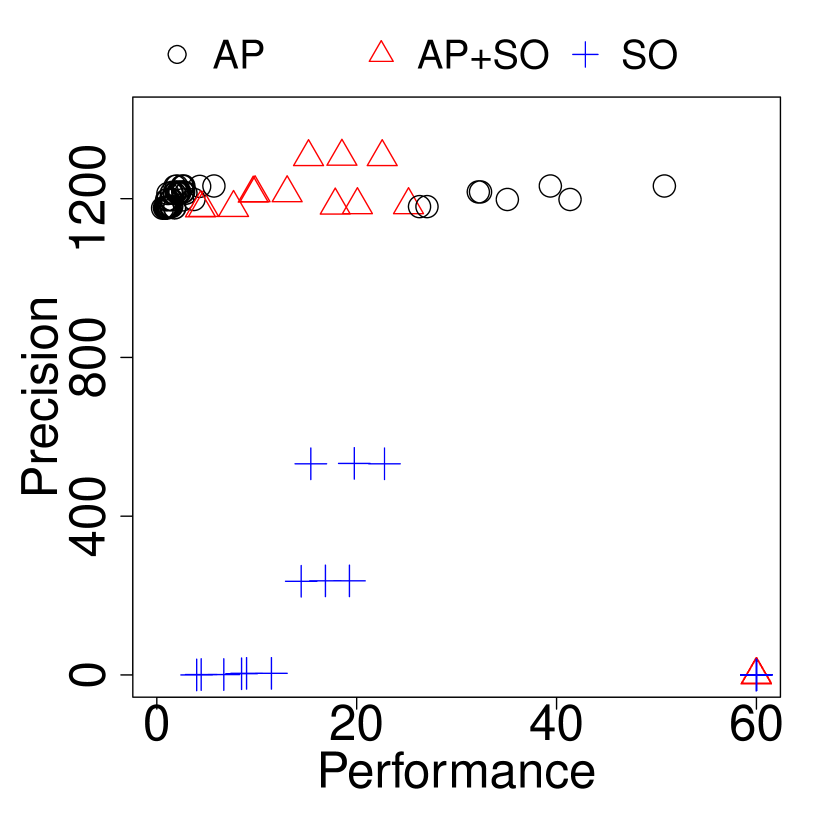
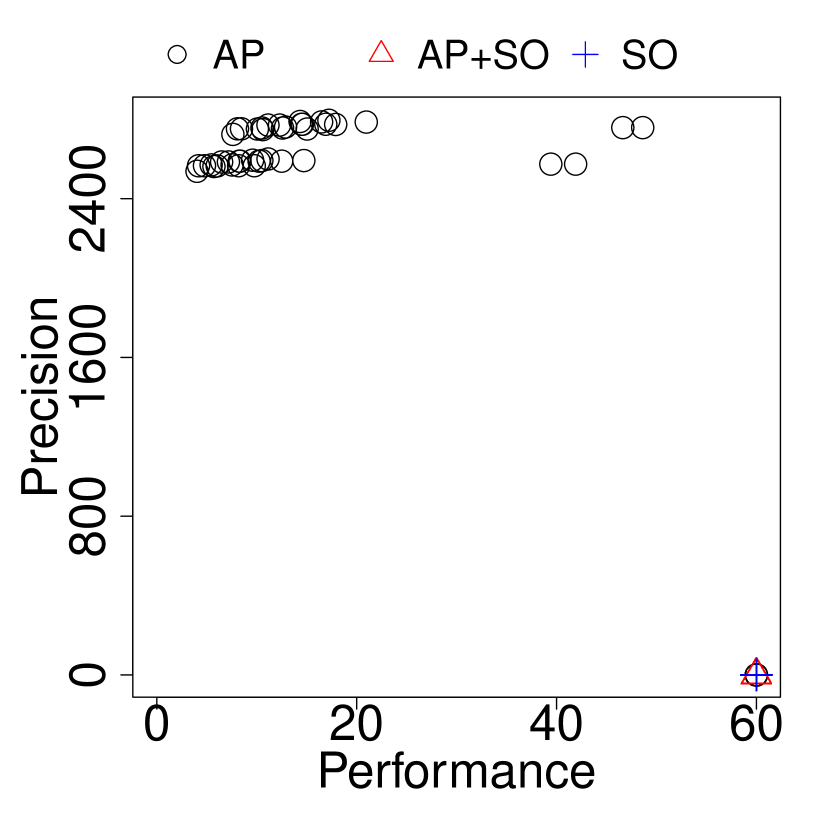
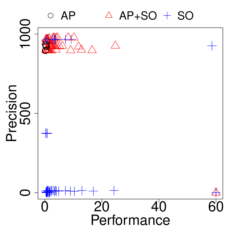
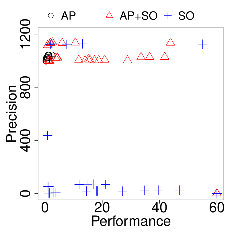
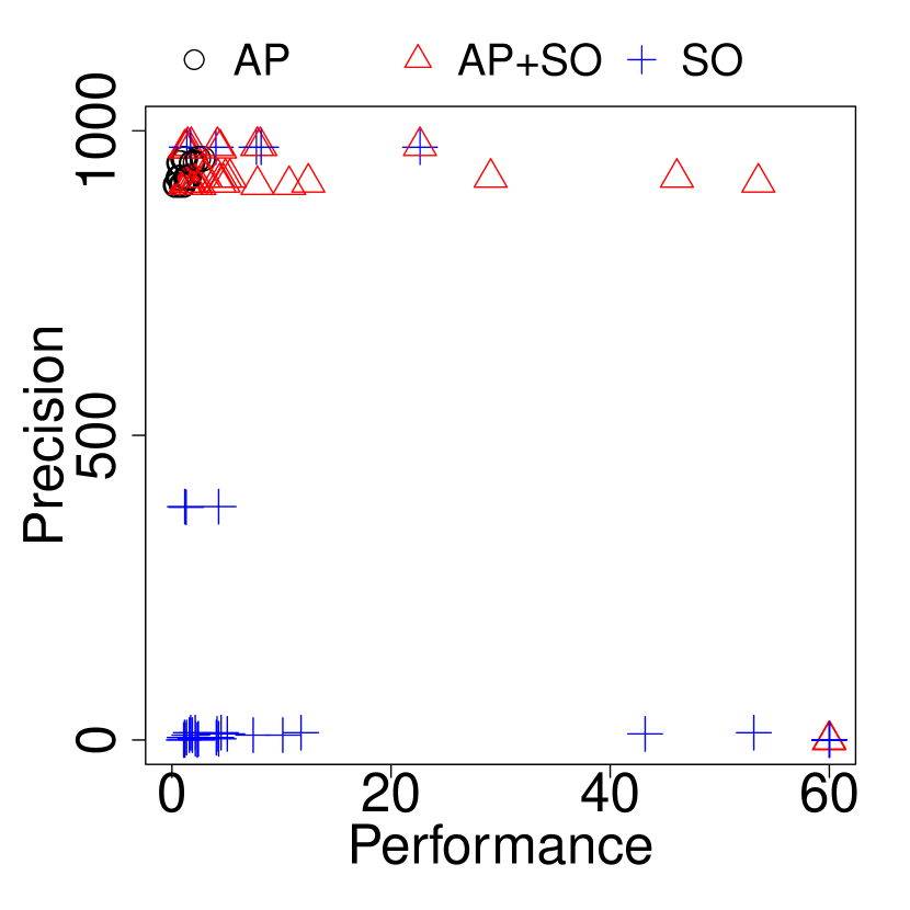
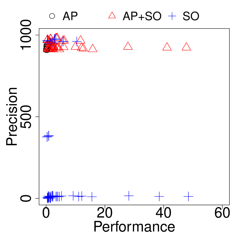
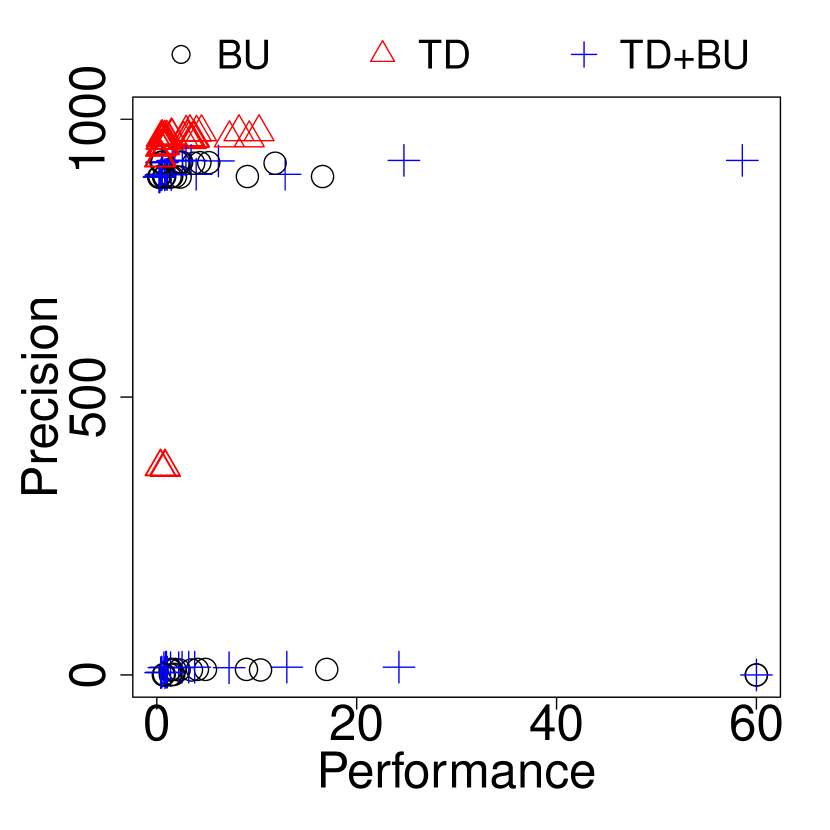
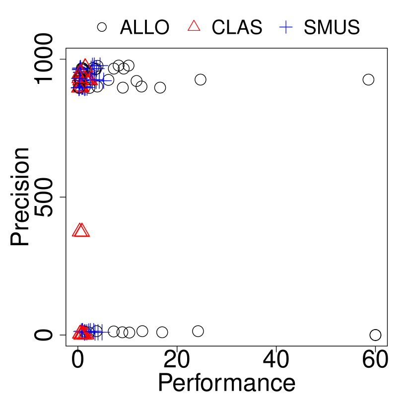
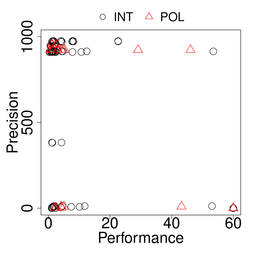
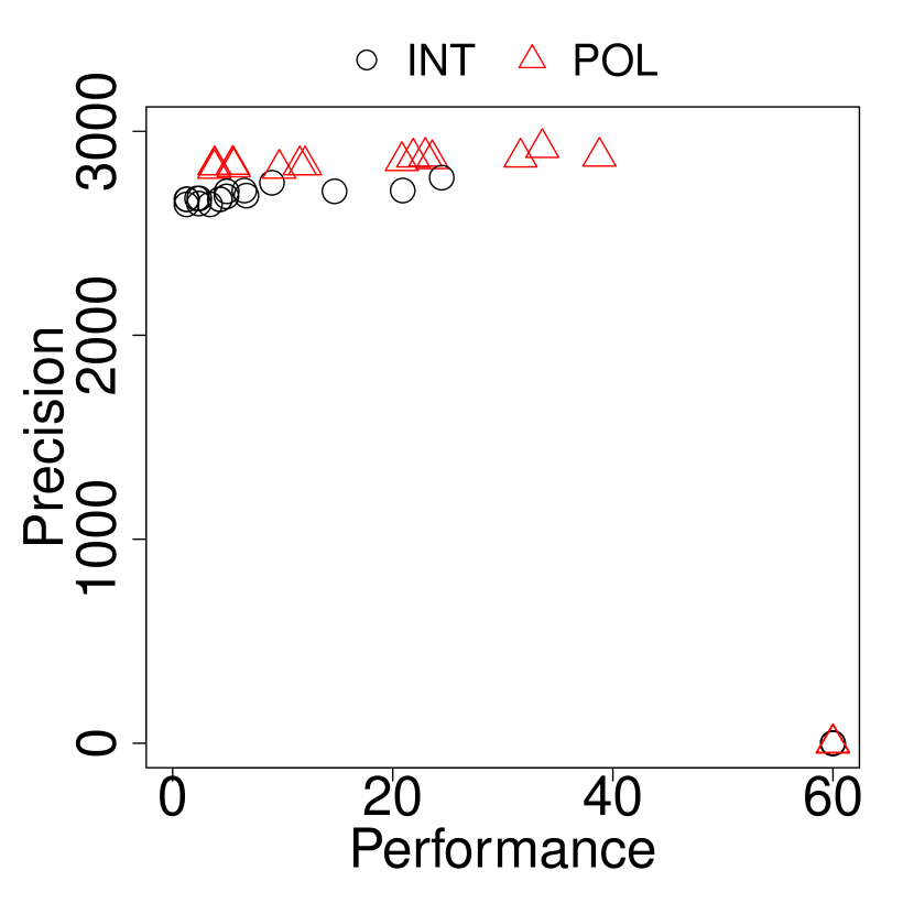
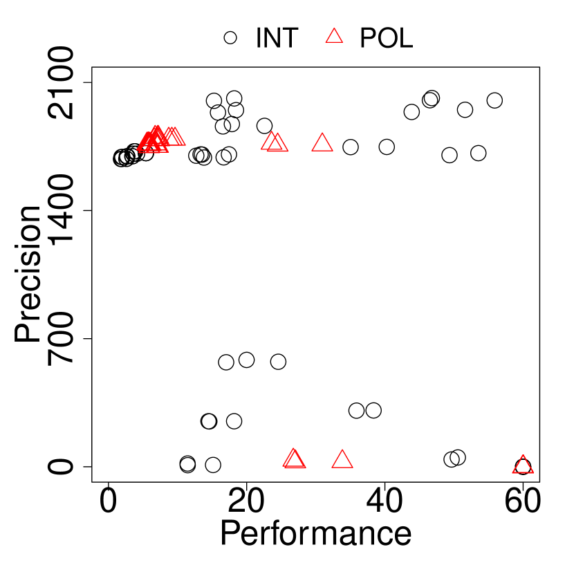
To delve further into the tradeoff, we examine, for each program, the overall performance and precision distribution for the analysis configurations, focusing on particular options (HA, AO, etc.). As settings of option HA have come up prominently in our discussion so far, we start with it and then move through the other options. Figure 1 gives per-benchmark scatter plots of this data. Each plotted point corresponds to one configuration, with its performance on the $x$-axis and number of discharged array bounds checks on the $y$-axis. We regard a configuration that times out as discharging no checks, so it is plotted at (60, 0). The shape of a point indicates the HA setting of the corresponding configuration: black circle for AP, red triangle for AP+SO, and blue cross for SO.

As a general trend, we see that access paths improve precision and do little to harm performance; they should always be enabled. More specifically, configurations using AP and AP+SO (when they do not time out) are always toward the top of the graph, meaning good precision. Moreover, the performance profile of SO and AP+SO is quite similar, as evidenced by related clusters in the graphs differing in the y-axis, but not the x-axis. In only one case did AP+SO time out when SO alone did not.

On the flip side, summary objects are a significant performance bottleneck for a small boost in precision. On the graphs, we can see that the black AP circles are often among the most precise, while AP+SO tend to be the best ($8/11$ cases in Table 2). But AP are much faster. For example, for bloat, chart, and jython, only AP configurations complete before the timeout, and for pmd, all but four of the configurations that completed use AP.

(a) antlr

(b) bloat

(c) chart

(d) eclipse

(e) fop

(f) hsqldb

(g) jython

(h) luindex

(i) lusearch

(j) pmd

(k) xalan

Figure 1: Tradeoffs: AP vs. SO vs. AP+SO.

(a) antlr

(b) bloat

(c) chart

(d) eclipse

(e) fop

(f) hsqldb

(g) jython

(h) luindex

(i) lusearch

(j) pmd

(k) xalan

Figure 2: Tradeoffs: TD vs. BU vs. TD+BU.

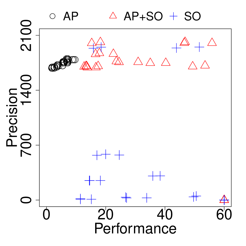
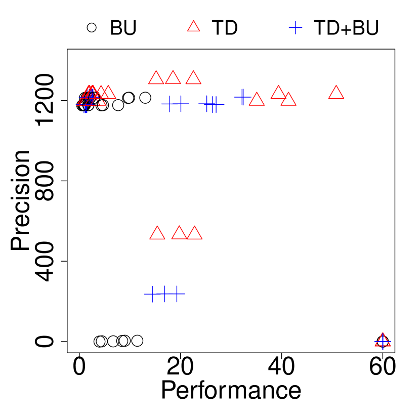
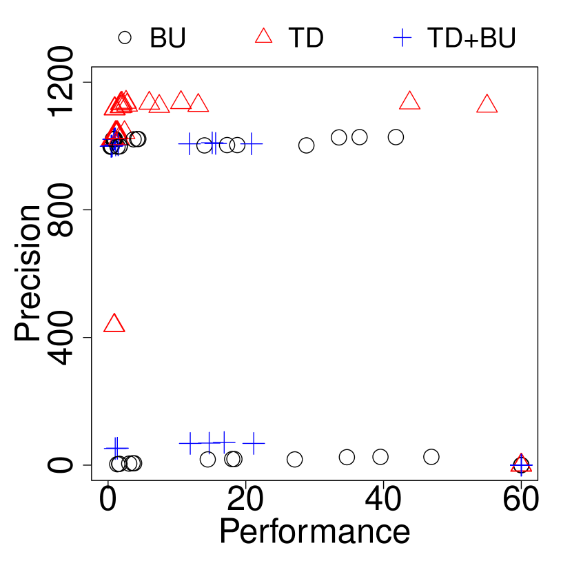
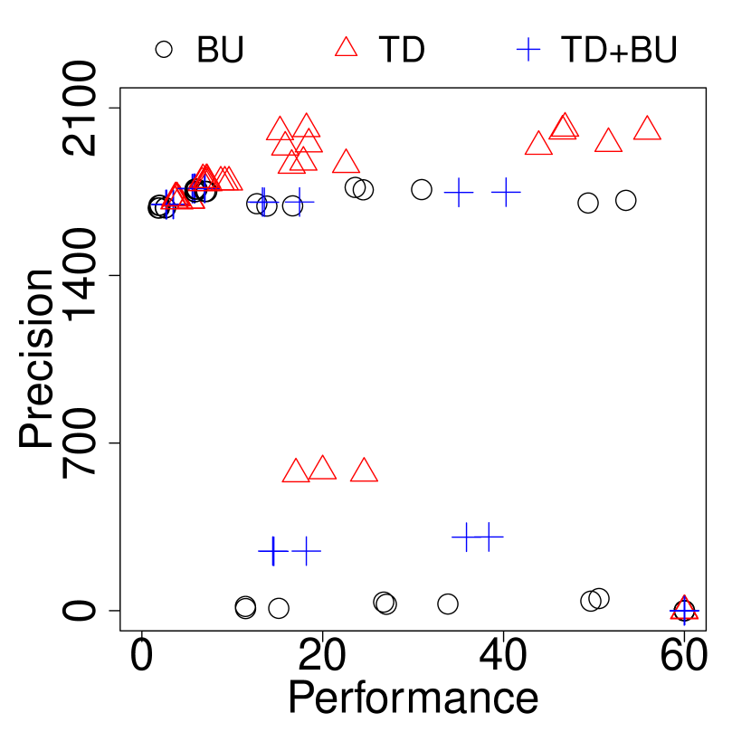
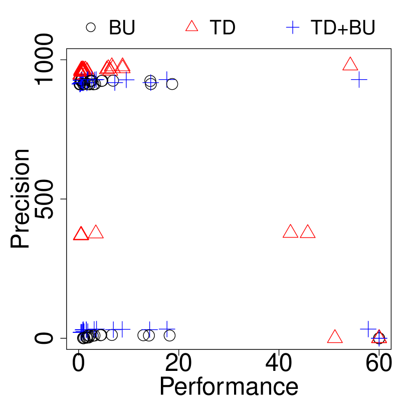
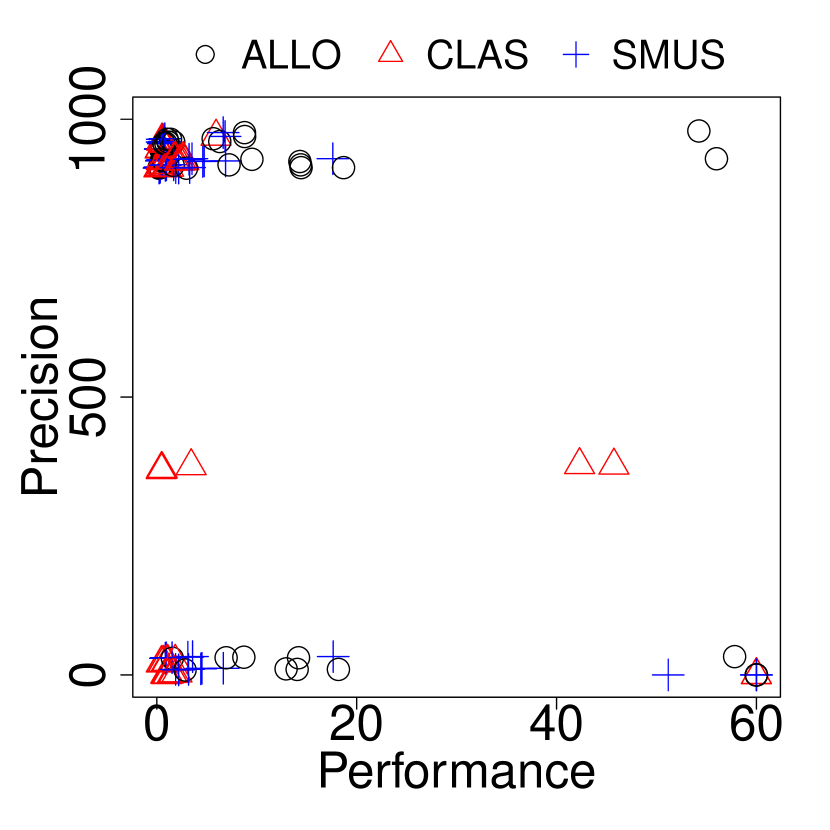
Top-down analysis is preferred: Bottom-up is less precise and does little to improve performance. Figure 2 shows a scatter plot of the precision/performance behavior of all configurations, distinguishing those with BU (black circles), TD (red triangles), and TD+BU (blue crosses). Here the trend is not as stark as with HA, but we can see that the mass of TD points is towards the upper-left of the plots, except for some timeouts, while BU and TD+BU have more configurations at the bottom, with low precision. By comparing the same (x,y) coordinate on a graph in this figure with the corresponding graph in the previous one, we can see options interacting. Observe that the cluster of black circles at the lower left for antlr in Figure 2(a) correspond to SO-only configurations in Figure 1(a), thus illustrating the strong negative interaction on precision of BU:SO we discussed in the previous subsection. The figures (and Table 2) also show that the best-performing configurations involve bottom-up analysis, but usually the benefit is inconsistent and very small. And TD+BU does not seem to balance the precision/performance tradeoff particularly well.

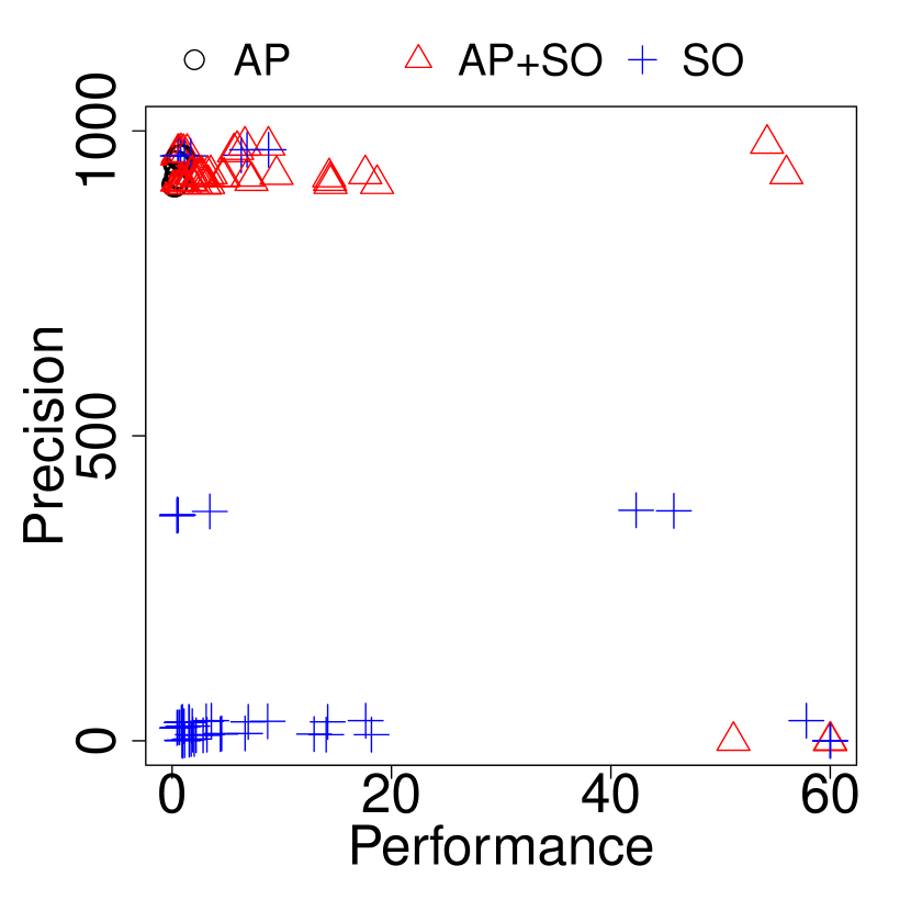
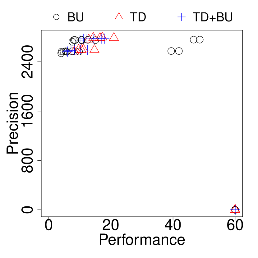
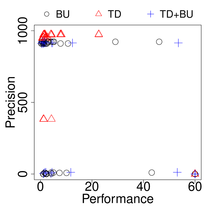
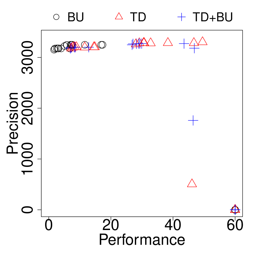
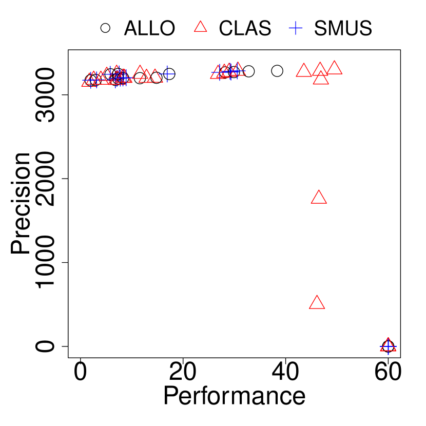
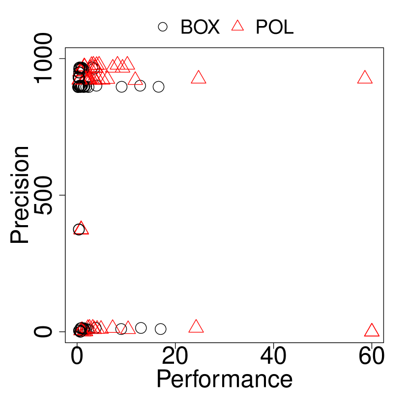
Precise object representation often helps with precision at a modest cost to performance. Figure 3 shows a representative sample of scatter plots illustrating the tradeoff between ALLO, CLAS, and SMUS. In general, we see that the highest points tend to be ALLO, and these are more to the right of CLAS and SMUS. On the other hand, the precision gain of ALLO tends to be modest, and these usually occur (examining individual runs) when combining with AP+SO. However, summary objects and ALLO together greatly increase the risk of timeouts and low performance. For example, for eclipse the row of circles across the bottom are all SO-only.

(a) eclipse

(b) lusearch

(c) pmd

Figure 3: Tradeoffs: ALLO vs. SMUS vs. CLAS.

(a) antlr

(b) bloat

(c) chart

(d) eclipse

(e) fop

(f) hsqldb

(g) jython

(h) luindex

(i) lusearch

(j) pmd

(k) xalan

Figure 4: Tradeoffs: INT vs. POL.

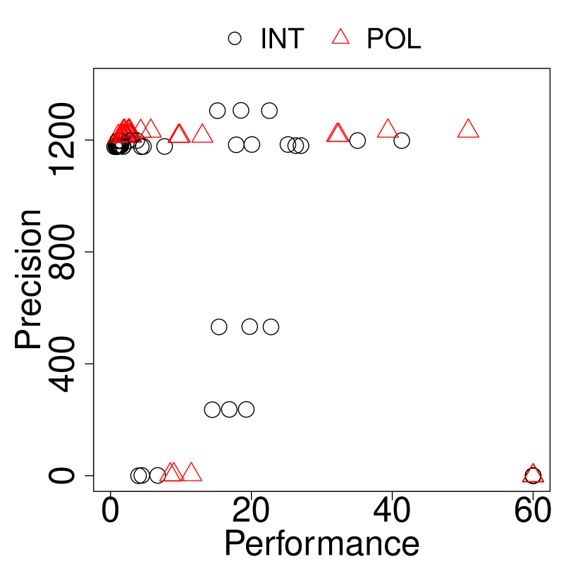
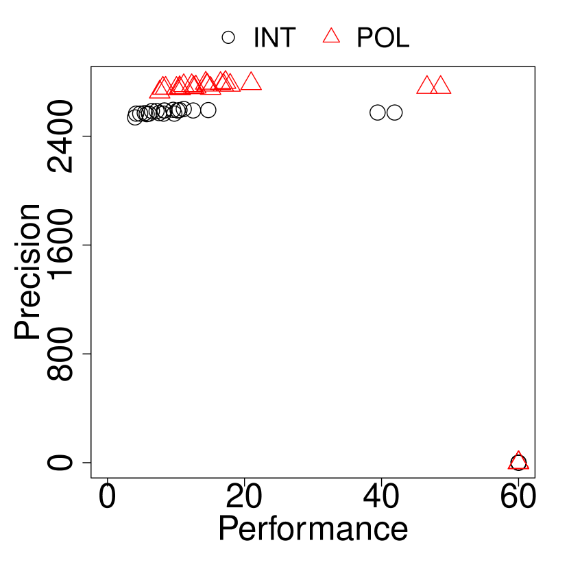
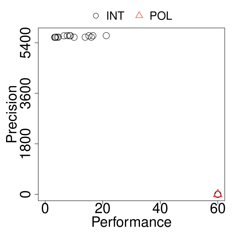
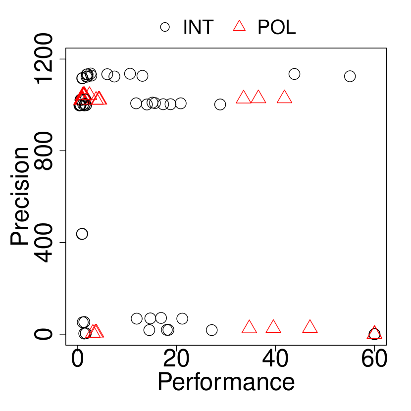
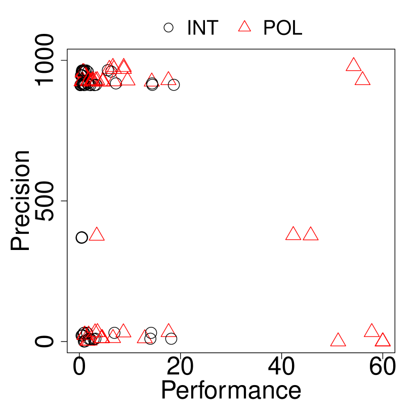
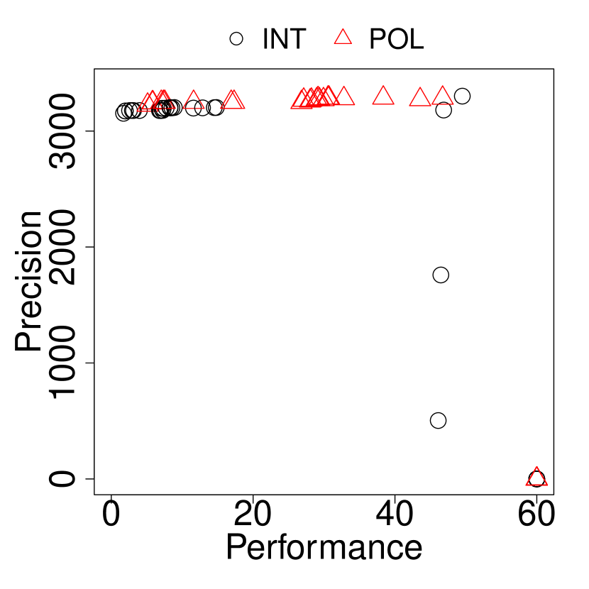
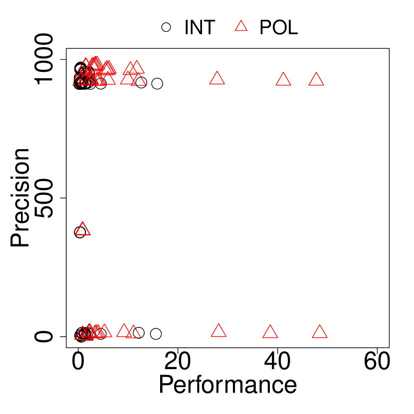
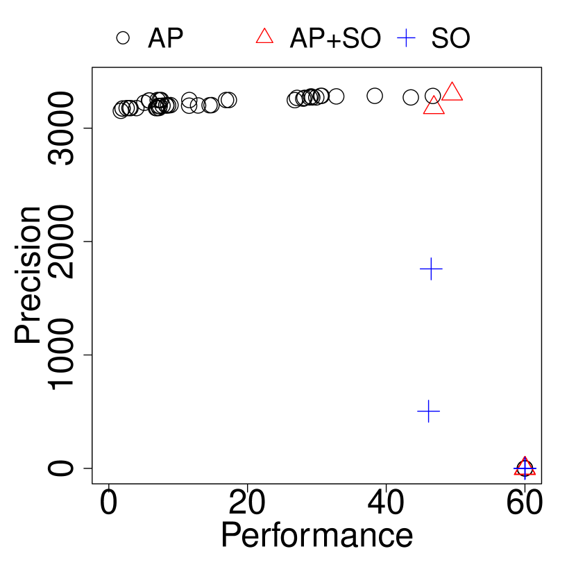
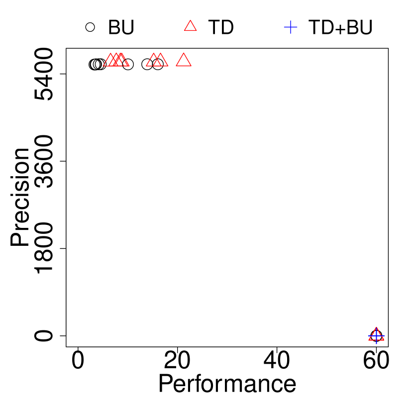
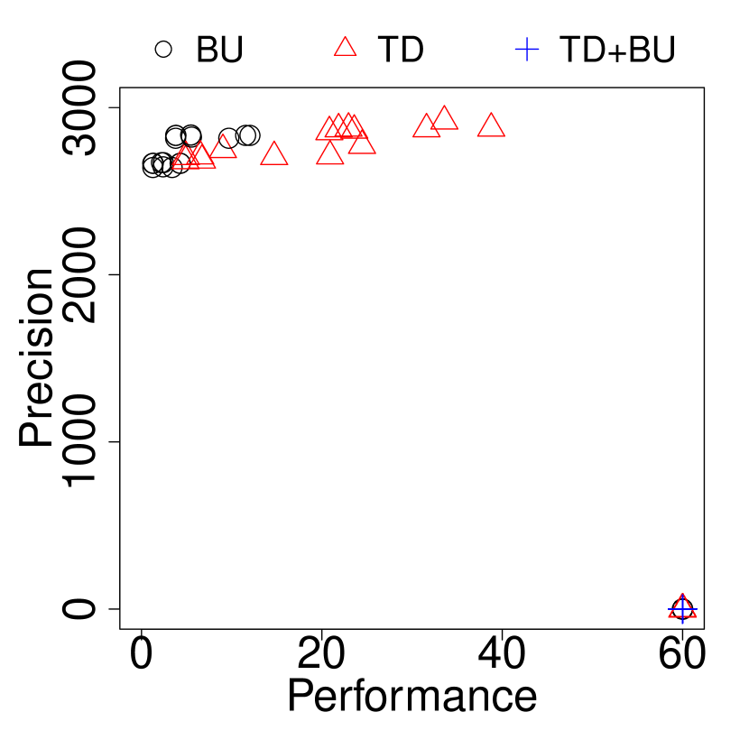
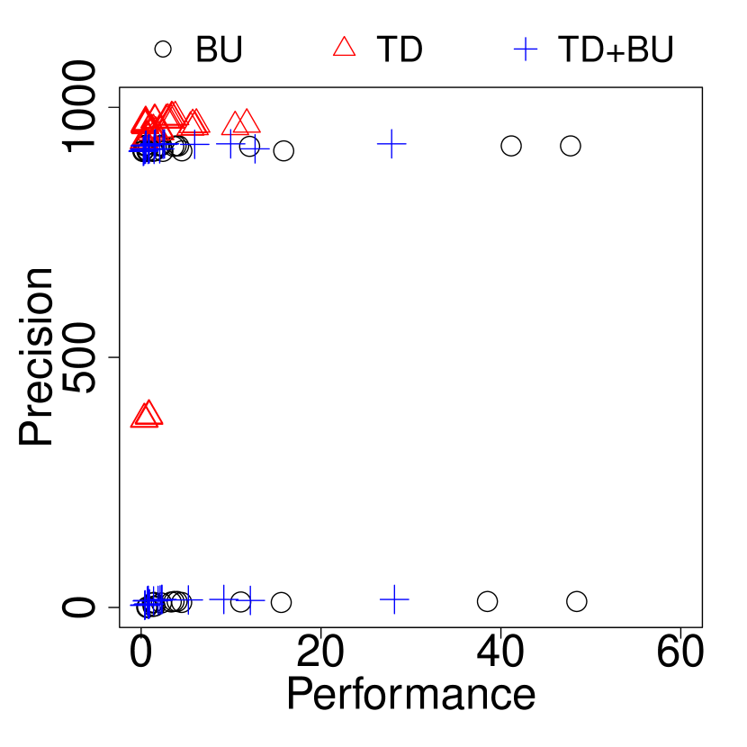
The precision gains of POLY are more modest than gains due to using AP+SO (over AP). Figure 4 shows scatter plots comparing INT and POLY. We investigated several groupings in more detail and found an interesting interaction between the numeric domain and the heap abstraction: POLY is often better than INT for AP (only). For example, the points in the upper left of bloat use AP, and POLY is slightly better than INT. The same phenomenon occurs in luindex in the cluster of triangles and circles to the upper left. But INT does better further up and to the right in luindex. This is because these configurations use AP+SO, which times out when POLY is enabled. A similar phenomenon occurs for the two points in the upper right of pmd, and the most precise points for hsqldb. Indeed, when a configuration with AP+SO-INT terminates, it will be more precise than those with AP-POLY, but is likely slower. We manually inspected the cases where AP+SO-INT is more precise than AP-POLY, and found that it mostly is because of the limitation that access paths are dropped through method calls. AP+SO rarely terminates when coupled with POLY because of the very large number of dimensions added by summary objects.

7 Related Work

Our numeric analysis is novel in its focus on fully automatically identifying numeric invariants in real (heap-manipulating, method-calling) Java programs, while aiming to be sound. We know of no prior work that carefully studies precision and performance tradeoffs in this setting. Prior work tends to be much more imprecise and/or intentionally unsound, but scale better, or more precise, but not scale to programs as large as those in the DaCapo benchmark suite.

Numeric vs. heap analysis.

Many abstract interpretation-based analyses focus on numeric properties or heap properties, but not both. For example, Calcagno et al. [13] uses separation logic to create a compositional, bottom-up heap analysis. Their client analysis for Java checks for NULL pointers [1], but not out-of-bounds array indexes. Conversely, the PAGAI analyzer [31] for LLVM explores abstract interpretation algorithms for precise invariants of numeric variables, but ignores the heap (soundly treating heap locations as $\top$).

Numeric analysis in heap-manipulating programs.

Fu [25] first proposed the basic summary object heap abstraction we explore in this paper. The approach uses a points-to analysis [47] as the basis of generating abstract names for summary objects that are weakly updated [27]. The approach does not support strong updates to heap objects and ignores procedure calls, making unsound assumptions about effects of calls to or from the procedure being analyzed. Fu’s evaluation on DaCapo only considered how often the analysis yields a non-$\top$ field, while ours considers how often the analysis can prove that an array index is in bounds, which is a more direct measure of utility. Our experiments strongly suggest that when modeled soundly and at scale, summary objects add enormous performance overhead while doing much less to assist precision when compared to strongly updatable access paths alone [21, 54].

Some prior work focuses on inferring precise invariants about heap-allocated objects, e.g., relating the presence of an object in a collection to the value of one of the object’s fields. Ferrera et al [23, 24] also propose a composed analysis for numeric properties of heap manipulating programs. Their approach is amenable to both points-to and shape analyses (e.g., TVLA [34]), supporting strong updates for the latter. Deskcheck [39] and Chang and Rival [14, 15] also aim to combine shape analysis and numeric analysis, in both cases requiring the analyst to specify predicates about the data structures of interest. Magill [37] automatically converts heap-manipulating programs into integer programs such that proving a numeric property of the latter implies a numeric shape property (e.g., a list’s length) of the former. The systems just described support more precise invariants than our approach, but are less general or scalable: they tend to focus on much smaller programs, they do not support important language features (e.g., Ferrara’s approach lacks procedures, Deskcheck lacks loops), and may require manual annotation.

Clousot [22] also aims to check numeric invariants on real programs that use the heap. Methods are analyzed in isolation but require programmer-specified pre/post conditions and object invariants. In contrast, our interprocedural analysis is fully automated, requiring no annotations. Clousot’s heap analysis makes local, optimistic (and unsound) assumptions about aliasing, while our approach aims to be sound by using a global points-to analysis.

Measuring analysis parameter tradeoffs.

We are not aware of work exploring performance/precision tradeoffs of features in realistic abstract interpreters. Oftentimes, papers leave out important algorithmic details. The initial Astreé paper [7] contains a wealth of ideas, but does not evaluate them systematically, instead reporting anecdotal observations about their particular analysis targets. More often, papers focus on one element of an analysis to evaluate, e.g., Logozzo [36] examines precision and performance tradeoffs useful for certain kinds of numeric analyses, and Ferrara [24] evaluates his technique using both intervals and octagons as the numeric domain. Regarding the latter, our paper shows that interactions with the heap abstraction can have a strong impact on the numeric domain precision/performance tradeoff. Prior work by Smaragdakis et al. [52] investigates the performance/precision tradeoffs of various implementation decisions in points-to analysis. Paddle [35] evaluates tradeoffs among different abstractions of heap allocation sites in a points-to analysis, but specifically only evaluates the heap analysis and not other analyses that use it.

8 Conclusion and Future Work

We presented a family of static numeric analyses for Java. These analyses implement a novel combination of techniques to handle method calls, heap-allocated objects, and numeric analysis. We ran the 162 resulting analysis configurations on the DaCapo benchmark suite, and measured performance and precision in proving array indexes in bounds. Using a combination of multiple linear regression and data visualization, we found several trends. Among others, we discovered that strongly updatable access paths are always a good idea, adding significant precision at very little performance cost. We also found that top-down analysis also tended to improve precision at little cost, compared to bottom-up analysis. On the other hand, while summary objects did add precision when combined with access paths, they also added significant performance overhead, often resulting in timeouts. The polyhedral numeric domain improved precision, but would time out when using a richer heap abstraction; intervals and a richer heap would work better.

The results of our study suggest several directions for future work. For example, for many programs, a much more expensive analysis often did not add much more in terms of precision; a pre-analysis that identifies the tradeoff would be worthwhile. Another direction is to investigate a more sparse representation of summary objects that retains their modest precision benefits, but avoids the overall blowup. We also plan to consider other analysis configuration options. Our current implementation uses an ahead-of-time points-to analysis to model the heap; an alternative solution is to analyze the heap along with the numeric analysis [46]. Concerning abstract object representation and context sensitivity, there are other potentially interesting choices, e.g., recency abstraction [5] and object sensitivity [40]. Other interesting dimensions to consider are field sensitivity [32] and widening, notably widening with thresholds. Finally, we plan to explore other effective ways to design hybrid top-down and bottom-up analysis [56], and investigate sparse inter-procedural analysis for better performance [45].

8.0.1 Acknowledgments.

We thank Gagandeep Singh for his help in debugging ELINA. We thank Arlen Cox, Xavier Rival, and the anonymous reviewers for their detailed feedback and comments. This research was supported in part by DARPA under contracts FA8750-15-2-0104 and FA8750-16-C-0022.

$$\begin{array}[]{l@{~~~~~~}lclr}\text{Num. Abstr.}\hfil~{}~{}~{}~{}~{}~{}&C&::=&\lx@intercol\text{constraints over }P,E\hfil\lx@intercol\\ \text{Exps}\hfil~{}~{}~{}~{}~{}~{}&e\in E&::=&x\mid n\mid e~{}\mathit{op}~{}e&\\ \text{Paths}\hfil~{}~{}~{}~{}~{}~{}&p\in P&::=&x\mid x.f\mid o.f&\\ \text{Variables}\hfil~{}~{}~{}~{}~{}~{}&x,y,z&\in&V&\\ \text{Field}\hfil~{}~{}~{}~{}~{}~{}&f,g&\in&F&\\ \text{Abstract Names}\hfil~{}~{}~{}~{}~{}~{}&o&\in&O&\\ \text{Points-to}\hfil~{}~{}~{}~{}~{}~{}&Pt&\in&P\rightarrow\mathcal{P}(O)&\\ \text{Classes}\hfil~{}~{}~{}~{}~{}~{}&\mathtt{A}&\in&A&\\ \text{Source Methods}\hfil~{}~{}~{}~{}~{}~{}&&&S&\\ \text{Abstract Contexts}\hfil~{}~{}~{}~{}~{}~{}&&&N&\\ \text{Methods in Context}\hfil~{}~{}~{}~{}~{}~{}&m&\in&S\times N&\\ \hfil~{}~{}~{}~{}~{}~{}\\ \text{Statements}\hfil~{}~{}~{}~{}~{}~{}&stmt&::=&x~{}\mathtt{:=}~{}e&\text{Assignment}\\ \hfil~{}~{}~{}~{}~{}~{}&&\mid&x~{}\mathtt{:=}~{}\mathtt{new~{}A}&\text{Allocation}\\ \hfil~{}~{}~{}~{}~{}~{}&&\mid&y~{}\mathtt{:=}~{}x.f&\text{Field Read}\\ \hfil~{}~{}~{}~{}~{}~{}&&\mid&x.f~{}\mathtt{:=}~{}e&\text{Field Write}\\ \hfil~{}~{}~{}~{}~{}~{}&&\mid&m(x)\{stmt;~{}\texttt{return}~{}e\}&\text{Method Def.}\\ \hfil~{}~{}~{}~{}~{}~{}&&\mid&x~{}\mathtt{:=}~{}m(y)&\text{Method Call}\\ \hfil~{}~{}~{}~{}~{}~{}&&\mid&\texttt{if }e\texttt{ then }stmt&\text{Conditional}\\ \hfil~{}~{}~{}~{}~{}~{}&&&\;\;\;\;\;\;\;\texttt{ else }stmt&\\ \end{array}$$

Figure 5: Analysis elements and formal language.

Appendix 0.A Heap-based Numeric Static Analysis

This section uses formal notation to carefully describe our family of heap-based numeric static analyses for Java. It aims to add further detail and rigor to the general design presented in Sections 2 and 3. Appendix 0.A—this section—focuses on handling the heap, with the next three subsections considering the ND, OR, and HA options from Table 1 (page 1), respectively. The next section discusses method calls, including the top-down and bottom-up variants, corresponding to option AO. It also discusses the effect of context-sensitive analysis, per option CS (adding detail to the basic design given in Section 4).

Figure 5 summarizes the elements of our analysis. The top half characterizes features of the analysis, while the bottom half gives a simplified language with which we describe the relevant aspects of our analyses. We do not cover the fixed-point computation aspect of abstract interpreters as it is standard. Instead we describe the formalism in terms of abstract transfer functions that underlie the fixed-point computation.

0.A.1 numeric domain (ND)

The core component of a numeric analysis is a numeric domain, which presents an API for implementing abstract states $C$. An abstract state represents a set of program states. An abstract state, or abstraction, $C$ is a set of dimensions paired with a set of constraints that constrain each dimension’s possible values. Dimensions typically represent numeric variables. Since our analysis considers the heap, dimensions are used to represent paths $p$, which include not just variables $x$, but also field addresses $x.f$, and (abstract) object field addresses $o.f$ where $o$ are abstract names, e.g., as determined by a point-to analysis (more on this below). We call a path $x.f$ an access path, as in previous analyses [21, 54]. We consider flow-sensitive analysis, which produces a distinct $C$ for each program point.

A variety of numeric domains have been developed, with different performance/precision tradeoffs [17, 19, 43, 36]. In our experiments, we use one of two standard numeric domains: intervals (INT) and convex polyhedra (POL). Intervals [17] describe sets of numeric states using inequalities of the form $p~{}\texttt{relop}~{}n$ where $p$ is a path, $n$ is a constant integer, and $\mathit{relop}$ is a relational operator such as $\leq$. Convex polyhedra [19] describe sets of numeric states using linear relationships between dimensions and constants, e.g., of the form $3p_{1}-p_{2}\leq 5$. Intervals are less precise but more efficient than polyhedra.

Example 1

Consider the following method.

⬇

1int f(int x) { //assume 0 $\leq$ x $\leq$ 10

2 int y1 = x + 10;

3 int y2 = x;

4 return y1 - y2;

5}

Suppose that $\texttt{x}\geq 0,\;\texttt{x}\leq 10$ at method entry. An interval-based analysis would determine that at the conclusion of the method (i.e., at line 4), $\texttt{y1}\geq 10,\;\texttt{y1}\leq 20$ and $\texttt{y2}\geq 0,\;\texttt{y2}\leq 10$. and infer constraints $\texttt{ret}\geq 0,\;\texttt{ret}\leq 20$ for the return value (here designated ret). This result is sound but imprecise. In contrast, a polyhedral analysis would determine that, at line 4, $\texttt{y1}=\texttt{x}+10,\;\texttt{y2}=\texttt{x},\;\texttt{ret}=\texttt{y1}-\texttt{y2}$ and thus (more precisely than the interval analysis) that $\texttt{ret}=10$.

operation	notation	description
interpret constraint	$[\!|{c}|\!]C$	Over-approximate constraint $c$ in the abstraction $C$.
project away	$C\setminus\left\{p_{1},\cdots\right\}$	$C$ with paths $p_{1},\cdots$ removed.
project to	$C\downarrow\left\{p_{1},\cdots\right\}$	$C$ with dimensions except those named by $p_{1},\cdots$ removed.
add constraints	$C\cup\left\{c,\cdots\right\}$	$C$ with additional constraints $\left\{c,\cdots\right\}$.
concatenate	$C_{1}\cup C_{2}$	Abstraction with constraints of both $C_{2}$ and $C_{1}$.
join	$C_{1}\sqcup{}C_{2}$	Join of abstractions $C_{1}$ and $C_{2}$. Join represents at least the concrete states represented by either $C_{1}$ or $C_{2}$.
strong update	$C[p\mapsto e]$	$C$ with strong update of $p$ made equal to $e$.
(dup) strong update	$C[p_{1}\mapsto_{\text{dup}}p_{2}]$	$C$ with a copy of $p_{2}$ constrained to be equal to $p_{1}$.
weak update	$C[p\hookrightarrow e]$	$C$ with weak update of $p$ made equal to $e$ or to what it was already.
(dup) weak update	$C[p_{1}\hookrightarrow_{\text{dup}}p_{2}]$	$C$ with a copy of $p_{2}$ weakly updated to be equal to at least $p_{1}$.

Figure 6: Operations on numeric abstractions. Interpret constraint returns a constraint while the other operations return a new abstraction.

Numeric domain operations. Several operations on numeric abstractions are important the formalism we present. An overview of these operations are shown in Figure 6. Some aspects of the implementations of these operations are discussed in Section 5.

The interpretation of a constraint $c$ in an abstraction $C$ is an over-approximation of the constraint representable in $C$’s domain. Over-approximation here means that if $c$ is true for some concrete state, then the approximation must also hold for it.

We often want to project away unneeded paths to improve the performance of abstract operations. Projecting away paths $\left\{p,\cdots\right\}$ from $C$, written $C\setminus\left\{p,\cdots\right\}$ (or $C\setminus p$ if only one path is projected away) drops $\left\{p,\cdots\right\}$ from $C$ while preserving any transitive constraints involving $\left\{p,\cdots\right\}$. For example, $(x\leq y,\;y\leq 5)\setminus y$ is $x\leq 5$. When we want to project away all paths except those in set $S$, we write $C\downarrow S$. Thus $(x\leq y,\;y\leq 5)\downarrow{}\{x\}$ is also $x\leq 5$.

Abstractions can be refined by adding constraints $\left\{c,\cdots\right\}$ or concatenating constraints from two abstractions, written $C\cup\left\{c,\cdots\right\}$ and $C_{1}\cup C_{2}$, respectively. For concatenation, we assume that the input abstractions are defined over disjoint sets of paths.

The join $C_{1}\sqcup C_{2}$ of two abstract states $C_{1}$ and $C_{2}$ produces an abstraction that over-approximates both. For example, given interval $C_{1}$ with constraint $x=10$ and interval $C_{2}$ with constraint $x=5$, their join, written $C_{1}\sqcup{}C_{2}$, is an abstraction with constraints $x\geq 5,\;x\leq 10$. (Notice the join has lost some precision because the domain of intervals cannot represent the combination any more precisely.)

Local assignments $x~{}\mathtt{:=}~{}e$ will be modeled by updating the input numeric abstraction $C$ so that $x$ is strongly updated to $e$, which we write as $C[x\mapsto e]$. The notation $C[x\mapsto e]$ is equivalent to $(C\setminus{}{x})\cup\{[\!|{x=e}|\!]C\}$, i.e., we project away $x$ and then add a single new constraint between $x$ and $e$, as interpreted in the abstract domain. A variant of strong update, written $C[p_{1}\mapsto_{\text{dup}}p_{2}]$, strongly updates $p_{1}$ to a copy of the dimension referred to by $p_{2}$. This makes sure that further refinements on $p_{1}$ and $p_{2}$ do not affect each other.

In several other rules, we write $C[p\hookrightarrow e]$ for a weak update of path $p$ to $e$, which is shorthand for $C\sqcup{}C[p\mapsto e]$, i.e., we join $C$, which may have existing constraints on $p$, with $C$ where $p$ is strongly updated to be $e$. As in strong update, a duplicating variant of weak update, written $C[p_{1}\hookrightarrow_{\text{dup}}p_{2}]$, weakly updates $p_{1}$ to a copy of the dimension referred to by $p_{2}$. This operation is equivalent to $C[p\mapsto_{\text{dup}}p_{2}][p_{1}\hookrightarrow p]\setminus p$ where $p$ is fresh.

0.A.2 abstract object representation (OR)

Traditionally, in a numeric abstraction, two distinct dimensions name two distinct memory locations. This means that if we assign $3$ to variable $x$, our numeric abstraction can strongly update $x$ to 3, leaving $y$ unaffected. But in a language with pointers, two distinct paths may point to the same memory. As such, assigning to $x.f$ might also affect path $y.f$ if $x$ and $y$ could be aliases.

To solve this problem we employ a points-to analysis [47], which computes (as shown in Figure 5) a map $Pt$ from paths $p$ to a set of abstract names $o$. An abstract name $o$ is a name that represents one or more concrete (run-time) heap-allocated objects. Importantly, if two have overlapping points-to sets, then they may alias. For example, if $o\in Pt(x)$ and $o\in Pt(y)$, then an assignment $x.f\;\texttt{:=}\;3$ must account for the impact on $y.f$ too. There are different ways to do this, as we discuss in the next subsection.

We consider three distinct ways to construct abstract names $o$ (which approach is used is elided from the formalism): (1) by allocation site (ALLO), where all objects allocated at the same syntactic program point share the same abstract name; (2) class-based (CLAS), where all objects of the same class share the same abstract name (i.e., they are conservatively assumed to alias); and (3) a hybrid smushed string (SMUS) approach, where every String object has the same abstract name but objects of other types have allocation site names. The allocation-site approach is the most precise, the class-based approach is less precise but potentially more efficient (since it will introduce fewer dimensions), and the smushed string analysis is somewhere in between.

0.A.3 heap abstraction (HA)

To handle programs that use fields, we must track paths in the abstract state, i.e., we must map a path like $x.f$ to a dimension in $C$. In addition to the problem of aliasing just mentioned (i.e., that an assignment such $x.f\;\texttt{:=}\;3$ may impact $y.f$ if $x$ and $y$ are aliases), there is also the problem that there is a conceptually unbounded number of memory locations. For example, in a linked list we might have path $l$, and $l.\texttt{next}$ and $l.\texttt{next}.\texttt{next}$, etc. and looping through the list means looping through these paths. For a static (i.e., finite) analysis, we need a single dimension that may represent many possible concrete memory locations.

A standard solution to this problem was presented by Gopan et al [27]: use a summary object to abstract information about multiple heap locations as a single dimension. A key question is how to map paths to summary object names. Fu [25] proposed doing this using the abstract names from points-to analysis. In particular, whenever performing a read or write on $x.f$, we construct a set of summary object names $\{o.f\mid o\in Pt(x)\}$ and perform the operation on those. We designate this approach as option SO.

While option SO is sound, it can be imprecise. Notably, all writes to summary objects must occur as weak updates. We can improve the situation by adding limited support for strong updates via access paths $x.f$. More specifically, after a write to $x.f$, we track its value separately from another objects potentially aliased with $x$, so that a subsequent read of $x.f$ will return the written value. If there is a potential conflicting write, e.g., to $y.f$ where $x$ and $y$ may alias, then we perform a weak update. An approach combining strongly-updatable access paths with summary objects we designate AP+SO, and a version that ignores summary object names $o.f$ altogether we designate AP.

In what follows, we present the AP+SO analysis first, then the AP and SO variants. These analyses are compatible with our top-down interprocedural analysis, presented in Section 0.B.1; variants compatible with bottom-up interprocedural analysis are given in Section 0.B.2.

Example 2

In the subsequent discussion, we illustrate the intraprocedural portion of our analysis using the following running example.

⬇

1int f() {

2 X x = new X();

3 int y1 = x.f;

4 x.f = 10;

5 int y2 = x.f;

6 return y1+y2;

7}

In this code, we assume X is some class with an integer field f. A points-to analysis of the program will produce a map $Pt$ with only $Pt($x$)=\{o_{x}\}$ for some abstract name $o_{x}$. The meaning of the abstract name varies depending on the type of points-to analysis but has on bearing on our analysis.

$$\begin{array}[]{c}\begin{array}[t]{ll}\begin{array}[t]{l}\text{Local assignment}\\ \underline{x~{}\mathtt{:=}~{}e}:\\ \quad C\leftarrow C[x\mapsto e]\\[4.30554pt] \end{array}&\begin{array}[t]{l}\text{Object allocation}\\ \underline{x~{}\mathtt{:=}~{}\mathtt{new~{}A}}:\\ \quad\forall\text{ numeric fields }\mathtt{A}.f_{i}.\\ \qquad C\leftarrow C[o.f\hookrightarrow 0]\;\forall o\in Pt(x)\\ \quad\text{call to {A}'s constructor is processed later}\\[4.30554pt] \end{array}\\ \\ \begin{array}[t]{l}\text{Field read}\\ \underline{y~{}\mathtt{:=}~{}x.f}:\\ \quad x.f\not\in C\Rightarrow\\ \quad\quad C\leftarrow C[x.f\hookrightarrow_{\text{dup}}o.f]\;\forall o\in Pt(x)\\ \quad C\leftarrow C[y\mapsto x.f]\\[4.30554pt] \end{array}&\begin{array}[t]{l}\text{Field write}\\ \underline{x.f~{}\mathtt{:=}~{}e}:\\ \quad C\leftarrow C[x.f\mapsto e]\\ \quad C\leftarrow C[o.f\hookrightarrow e]\;\forall o\in Pt(x)\\ \quad C\leftarrow C[z.f\hookrightarrow e]\;\forall z\text{ with }Pt(x)\cap Pt(z)\not=\emptyset\\[4.30554pt] \end{array}\\ \\ \end{array}\\ \begin{array}[t]{l}\text{Conditional}\\ \underline{\text{if}~{}e~{}\text{then}~{}s_{1}~{}\text{else}~{}s_{2}}:\\ \quad C_{t}\leftarrow[\!|{s_{1}}|\!]\left(C\cup{[\!|{e=\text{true}}|\!]C}\right)\\ \quad C_{f}\leftarrow[\!|{s_{2}}|\!]\left(C\cup{[\!|{e=\text{false}}|\!]C}\right)\\ \quad C\leftarrow C_{t}\sqcup{}C_{f}\\[4.30554pt] \end{array}\\ \end{array}$$

Figure 7: Basic abstract transfer functions for summary and access paths (AP+SO) heap abstraction (HA).

0.A.3.1 AP+SO analysis

Figure 7 summarizes the abstract transfer functions for AP+SO. Operating on abstractions $C$ of concrete states, each transfer function over-approximates the concrete semantics of particular statement. We assume that $C$ is the analysis’ current abstract state (e.g., due to the previous statement). We then write $C\leftarrow...$ to mean we update that state so that it captures the effect of the current statement.

Local assignment

The assignments $x~{}\mathtt{:=}~{}e$ are modeled by updating the input numeric abstraction $C$ so that $x$ is strongly updated to $e$, written $C[x\mapsto e]$.

Object allocation

$x~{}\mathtt{:=}~{}\texttt{new~{}A}$, considers all abstract names $o$ in $Pt(x)$ and weakly updates $o.f$ to $0$, the default int value. In our example, this adds $o_{x}.f=0$ to $C$. In our implementation, we model non-default constructors by subsequently invoking them like a method call.

To demonstrate the field read and write transfer functions, we step through the analysis of Example 2.

Field read (no access path)

Consider line 3 of Example 2, which reads x’s numeric field f and stores the result in y1.Since this is the first time we have read x.f, we have not created an access path for it (so $x.f\not\in C$). Therefore, we need to read field $f$ of each abstract object in $o\in{}Pt(x)$.

Recall that in general, an abstract location may represent multiple run-time objects [27] (even though it does not in our example), so we cannot be sure that any other read from the same abstract name refers to the same run-time object. Because of this, in top-down analysis, we weakly update the path x.f to copies of o.f, for every abstract name o that could alias with x. This copying makes sure that any subsequent read from shared abstract names will not be forced to be equal to x.f. After x.f is constructed, we strongly update the left-hand side of the assignment to it. In Example 2 the update will result in the constraints $\texttt{x.f}=0,\;\texttt{y1}=\texttt{x.f},\;o_{x}.\texttt{f}=0$.

The transfer function in the figure also supports the simpler case when $x.f\in C$. In this case, there must have been a strong update to $x.f$ previously, and so all information about $x.f$ is represented directly in the constraints. Thus, we need only strongly update $y$ with $x.f$. Line 5 in our example covers this case, strongly updating y2 to x.f.

As shown, the transfer function does not handle a statement $y~{}\mathtt{:=}~{}x.f$ when $x.f$ is an object rather than a numeric quantity. In this case, our implementation projects away any access paths $y.g$ from $C$, since the object pointed to by $y$ is now different. No further work is required as, when $y$ is referenced in the future, the analysis will use $Pt(y)$ to determine the objects $y$ points to.

Field assignment

Next in our running example, Line 4 performs a field write $\texttt{x.f}\;\texttt{:=}\;10$. The general rule is shown in the lower right of Figure 7. First, we strongly update the access path $x.f$ to the right-hand side of the assignment. In our example the constraints $\texttt{x.f}=0,\;\texttt{y1}=\texttt{x.f},\;o_{x}.\texttt{f}=0$ are transformed into $\texttt{x.f}=10,\;\texttt{y1}=0,\;o_{x}.\texttt{f}=0$. Then for all $o\in{}Pt(x)$, we weakly update all pointers $o.f$ to the right-hand side of the assignment. In our example, this joins $o_{x}.\texttt{f}=10$ with the prior constraint $o_{x}.\texttt{f}=0$ to yield $\texttt{x.f}=10,\;\texttt{y1}=0,\;0\leq o_{x}.\texttt{f}\leq 10$. Finally, we weakly update all access paths $z.f$ where $Pt(x)\cap Pt(x)\neq\emptyset$. In our example, we have no other access paths so no work is done.

At the end of our example function the constraints are $\texttt{x.f}=10,\;\texttt{y1}=0,\;0\leq o_{x}.\texttt{f}\leq 10,\;\texttt{y2}=10$. Hence when analyzing the last line of our example, we can infer that the returned result y1+y2 is $10$.

Control constructs

The last transfer function in Figure 7 illustrates the handling of conditionals. There, the true and false branches of a conditional are analyzed with interpretations of the guard condition being true or false, respectively, added to the abstraction’s constraints. The numeric domain used determines the precision of the interpretation of the guards. For loops, we employ a fixed-point computation and the numeric domain’s standard widening operator [4] in place of join to guarantee convergence within a finite number of iterations.

0.A.3.2 SO only

$\begin{array}[]{l}\text{Field read (Summary-only)}\\ \underline{y~{}\mathtt{:=}~{}x.f}:\\ \quad C\leftarrow C\setminus y\\ \quad C\leftarrow C[y\hookrightarrow_{\text{dup}}o.f]\;\forall o\in Pt(x)\end{array}$

$\begin{array}[]{l}\text{Field write (Summary-only)}\\ \underline{x.f~{}\mathtt{:=}~{}e}:\\ \quad C\leftarrow C[o.f\hookrightarrow e]\;\forall o\in Pt(x)\\ {}\\ \end{array}$

Figure 8: Transfer functions for summary-object only (SO) heap abstraction (HA) under top-down (TD) inter-procedural analysis order (AO).

The analysis presented to this point has combined access paths $x.f$ and heap locations $o.f$. We also implemented alternatives that just do one or the other. In the SO (“only heap locations”) analysis we do not track paths $x.f$. This means that field reads and writes are handled differently; the changes are shown in Figure 8. For the $y~{}\mathtt{:=}~{}x.f$ case, we simply initialize $y$ to be the join of all $o.f$ where $o\in Pt(x)$. For the $x.f~{}\mathtt{:=}~{}e$ case, we simply do a weak update to $o.f$ for all $o\in Pt(x)$.

$$\begin{array}[]{l}\text{Field read (Access-only)}\\ \underline{y~{}\mathtt{:=}~{}x.f}:\\ \quad C\leftarrow C[x.f\mapsto\top]\text{ if }x.f\not\in C\\ \quad C\leftarrow C[y\mapsto x.f]\end{array}$$

$$\begin{array}[]{l}\text{Field write (Access-only)}\\ \underline{x.f~{}\mathtt{:=}~{}e}:\\ \quad C\leftarrow C[x.f\mapsto e]\\ \quad C\leftarrow C[z.f\hookrightarrow e]\;\forall z\text{ with }Pt(x)\cap Pt(z)\not=\emptyset\end{array}$$

Figure 9: Transfer functions for access paths only (AP) heap abstraction (HA).

0.A.3.3 AP only

The AP (“only access paths”) analysis tracks access paths $x.f$ but does not specifically track heap locations $o.f$; in effect these are always assumed to be $\top$. The changes are shown in Figure 9. In essence, reading from a heap location for which there is no access path produces $\top$. Writing to an access path initializes that access path, but it may invalidate other, aliased access paths. Note that no changes are required to the algorithms for handling method calls—any parts that refer to locations $o.f$ will be vacuous since $o.f\not\in C$ for any $o.f$ and $C$.

Appendix 0.B Interprocedural Analysis

Now we consider inter-procedural analysis order (AO). We have implemented two main algorithms, top-down (TD) and bottom-up (BU), as well as a hybrid (TD+BU).

Example 3

We use the following example to illustrate our analyses.

⬇ 1int g() { 2 X xx1 = new X(); 3 X xx2 = new X(); 4 return f2(xx1, xx2, 10); 5}

⬇ 1int f2(X x1, X x2, int d) { 2 x1.f = d; 3 int y1 = x1.f; 4 int y2 = x2.f; 5 return y1+y2; 6}

Method f2 is a generalization of f from Example 2 that swaps the first two lines, uses two X objects x1 and x2 rather than a single x, and takes these objects as parameters, initialized in the caller rather than f itself. An allocation-based points-to analysis for this program would produce $Pt(\texttt{x1})=Pt(\texttt{xx1})=\{o_{1}\}$ and $Pt(\texttt{x2})=Pt(\texttt{xx2})=\{o_{2}\}$.

$$\begin{array}[t]{l}\text{Method call (Top-down)}\\ \underline{x~{}\mathtt{:=}~{}m(y)}:\\ \quad\text{where $m$ has formal $y_{m}$ and body $\{s;\mathtt{return}~{}e\}$}\\ \quad C_{m}\leftarrow C[y_{m}\mapsto y]\downarrow(\{y_{m}\}\cup\{o.f\mid o.f\in C\wedge o\in\mathit{refs}({m})\})\\ \quad C_{c}\leftarrow C\downarrow(\{o.f\mid o.f\in C\wedge o\not\in\mathit{refs}({m})\}\cup\{z\mid z\in C\}\text{ (for all local vars $z$)})\\ \quad C_{m}\leftarrow[\!|{s}|\!]C_{m}\\ \quad C_{m}\leftarrow C_{m}[\mathtt{ret}_{m}\mapsto e]\downarrow(\{\mathtt{ret}_{m}\}\cup\{o.f\mid o.f\in C_{m}\})\\ \quad C\leftarrow(C_{c}\cup C_{m})[x\mapsto\mathtt{ret}_{m}]\setminus\mathtt{ret}_{m}\\[4.30554pt] \end{array}$$

Figure 10: Transfer function for method invocation in top-down (TD) inter-procedural analysis order (AO). Caller is method $c$, callee is method $m$.

0.B.1 top-down (TD)

Our TD transfer function for analyzing a method call is shown in Figure 10. This function works for all three variants of the heap abstraction (AP, SO, and AP+SO) previously discussed. For simplicity we assume that return occurs as the last statement of a method. We also assume the single parameter $y$ is numeric; we consider object parameters shortly.

The first step is to construct an abstraction $C_{m}$ for the method $m$ being called. It consists of $C$ but with $m$’s parameter $y_{m}$ strongly updated to the actual argument $y$. After updating the formal $y_{m}$ with the actual $y$, we project away all but $y_{m}$ and any heap locations $o.f$ that are used by $m$ (or its callees). We do this projection because retaining the local variables and access paths of the caller when analyzing the callee can quickly become prohibitively expensive, especially for polyhedral abstractions.

Next, we define $C_{c}$ to hold only the caller’s local variables, dropping any access paths and heap locations used in the callee; we drop the former due to potential writes to them in the callee (via aliases). Then we update $C_{m}$ by analyzing the callee’s body $s$, written $C_{m}\leftarrow[\!|{s}|\!]C_{m}$. To process the return, we strongly update special local variable $\texttt{ret}_{m}$, and then project away all but this variable and any heap locations $o.f$. Finally, we concatenate callee’s abstraction $C_{c}$ with the final abstraction of the callee, $C_{m}$ (the paths in each will be disjoint) and strongly update the caller’s $x$ before projecting away $\texttt{ret}_{m}$.

In general, we use the call graph (informed by the points-to analysis) to determine possible callees. When there is more than one possible (e.g., due to dynamic dispatch) we perform the above steps for each callee, and then join the resulting abstractions.

Handling object parameters.

Consider methods that have object (not numeric) parameters (e.g., xx1 and xx2 in Example 3). For the SO variant, we do not constrain object parameters to methods specifically because the necessary information is already captured in the points-to analysis. So the description in Figure 10 is complete in this case.

For AP and AP+SO we refine our approach to perform access path inlining. In particular, we propagate access paths to the callee and back when they are arguments to a method call. In particular, for a call $m(x)$ where $m$’s parameter $x_{m}$ is an object and the caller has an access path $x.f$, we translate information about $x.f$ to the callee; i.e., constraints about $x.f$ in $C$ are used to initialize a path $x_{m}.f$ in $C_{m}$ similarly to $y_{m}$ and $y$ in the Figure. Moreover, as long as $x_{m}$ is never overwritten in $m$, we can map its current state back to the caller’s path $x.f$ at the conclusion of $m$.

Example.

Consider analyzing Example 3 with the TD analysis using heap abstraction AP+SO. We start with g. Analyzing lines 2 and 3 adds constraints $o_{1}.\texttt{f}=0$ and $o_{2}.\texttt{f}=0$ to $C$ and likewise $\texttt{xx1.f}=0$ and $\texttt{xx2.f}=0$. Then we analyze the call to f2. We set $C_{f2}$ to $C$ but after adding $\texttt{d}=10$ and translating access paths involving xx1 and xx2, respectively, to $\texttt{x1.f}=0$ and $\texttt{x2.f}=0$. We then define $C_{c}$ to save the caller’s locals; since $C$ contains none, $C_{c}$ ends up being empty.

Next we analyze f2 with initial abstraction $C_{f2}$. We handle line 2 of f2 by updating the access path for x1.f and setting it to 10. We weakly update $o_{1}.\texttt{f}$, adding constraints $o_{1}.\texttt{f}\geq 0,\;o_{1}.\texttt{f}\leq 10$. We handle line 3 by reading directly from the access path, setting $\texttt{y1}=\texttt{x1.f}$. Line 4 is similar to the handling of line 3 in Example 2, but using $o_{2}$ rather than $o_{x}$. At line 5, the returned result, 10, is assigned (via a strong update) to special local variable $\texttt{ret}_{f2}$.

Now that we are finished we project away from $C_{f2}$ all of f2’s local variables, aside from $\texttt{ret}_{f2}$. Access paths x1.f $=10$ and x2.f $=0$ are mapped back to access paths in the caller, xx1.f $=10$ and xx2.f $=0$. Since there were no numeric locals to save in the caller, $C_{f2}$ is used there as is (i.e., $C_{c}\cup C_{f2}=C_{f2}$). In it, we strongly update ret_g (i.e., the local variable in the caller receiving the result of the call) to ret_f2. We finally project away ret_f2, yielding ret_g $=$ 10.

$$\begin{array}[]{l}\text{Field read}\\ \underline{y~{}\mathtt{:=}~{}x.f}:\\ \quad x.f\not\in C\Rightarrow\\ \quad\quad\forall o\in Pt(x).\\ \quad\qquad C\leftarrow C[x.f\hookrightarrow o.f\_i_{c}]\text{ where }o.f\_i_{c}\text{ fresh}\\ \quad\qquad C\leftarrow C[x.f\hookrightarrow_{\text{dup}}o.f_{c}]\text{ if }o.f_{c}\in C\text{~{}~{}(i.e., same as Fig~{}\ref{fig:analysis})}\\ \quad C\leftarrow C[y\mapsto x.f]\end{array}$$

$$\begin{array}[]{l}\text{Method summary}\\ \underline{c(z)\{s;~{}\mathtt{return}~{}e\}}:\\ \qquad\text{where $z$ is method $c$'s param. }\\ \qquad\text{and $s$ is its body }\\ \quad C_{c}\leftarrow\left\{z=\top\right\}\\ \quad C_{c}\leftarrow[\!|{s}|\!]C_{c}\\ \quad C_{c}\leftarrow C_{c}[\mathtt{ret}_{c}\mapsto e]\\ \quad C_{c}\leftarrow C_{c}\downarrow(\{\mathtt{ret}_{c},z\}\cup\\ \quad\quad\quad\{o.f_{c},o.f\_i_{c}\mid o.f_{c},o.f\_i_{c}\in C_{c}\})\\ \text{$C_{c}$ becomes $c$'s summary}\\ \end{array}$$

$$\begin{array}[]{l}\text{Method call}\\ \underline{x~{}\mathtt{:=}~{}m(y)}:\\ \quad C\leftarrow C_{m}\cup C\text{ where $C_{m}$ is $m$'s summary}\\ \quad C\leftarrow C\cup\left\{z=y\right\}\text{ where $z$ is $m$'s formal param.}\\ \quad\forall o.f\_i_{m}\in C_{m}.\\ \quad\quad C\leftarrow C[o.f\_i_{m}\mapsto_{\text{dup}}o.f_{c}]\text{ if }o.f_{c}\in C\\ \quad\quad C\leftarrow C[o.f\_j_{c}\hookrightarrow o.f\_i_{m}]\text{ where $o.f\_j_{c}$ fresh}\\ \quad C\leftarrow C[o.f_{c}\hookrightarrow o.f_{m}]\;\forall o.f_{m}\in C_{m}\\ \quad C\leftarrow C[x\mapsto\mathtt{ret}_{m}]\\ \quad C\leftarrow C\setminus\{p\mid p\in C_{m}\}\end{array}$$

Figure 11: Transfer functions for bottom-up (BU) inter-procedural analysis order (AO) (access paths only (AP) and summary and access paths (AP+SO)).

0.B.2 bottom-up (BU)

Figure 11 describes the key features of our BU analysis. In this analysis we start at the leaves of the call tree, analyzing callees before callers. For each method $m$ we produce a summary numeric abstraction $C_{m}$. When $m$ is called, we instantiate $C_{m}$ in the caller’s context. To make this work, paths $o.f$ are annotated with the name of the method being analyzed; we call this annotation the frame. In the figure, we assume we are analyzing some method $c$, so paths $o.f$ and $o.f\_i$ are written $o.f_{c}$ and $o.f\_i_{c}$, respectively. We now explain the analysis using Example 3.

Callee analysis.

We begin analysis of f2 with $C_{f2}$ as the empty abstraction. We add the int parameter d as a (unconstrained) numeric variable to $C_{f2}$. We do nothing with x1 and x2 at first, as they are modeled by the points-to analysis. At line 2, we act similarly to the TD analysis: we compute $Pt(\texttt{x1})=\{o_{1}\}$, generate a fresh path $o_{1}.\texttt{f}_{f2}$ since it does not currently exist, weakly update it by adding constraint $o_{1}.\texttt{f}_{f2}=\texttt{d}$, and then generate and set access path $\texttt{x1.f}=\texttt{d}$. At line 3 we read x1.f using the rule in the upper-left of Figure 11(a). Since there is an access path x1.f, we simply generate constraint $\texttt{y1}=\texttt{x1.f}$, which is the same as the TD analysis.

At line 4, we read x2.f, hence we use the field read rule again. However, this time x2.f does not yet exist in $C_{f2}$. As in the TD analysis, we need to read field f of each $o\in Pt(\texttt{x2})$. In the TD analysis, we would duplicate the initial information about those $o.\texttt{f}$’s. However, we cannot do so in the BU analysis because we have not yet analyzed the caller. Instead, following the modified Field read rule in Figure 11, we first introduce a fresh location $o.\texttt{f}\_i_{c}$ standing for the initial contents of $o.\texttt{f}_{c}$ and weakly update x2.f with it. In this case, since $Pt(\texttt{x2})=\{o_{2}\}$, this results in the constraint $\texttt{x2.f}=o_{2}.\texttt{f}\_1_{c}$. Later on, when we call this method, we will initialize $o_{2}.\texttt{f}\_1_{c}$ from the caller (see below), and hence that initial information from the caller will be propagated to x2.f. Note that if there were multiple reads of x2.f, each would result in a new $o_{2}.\texttt{f}\_i_{c}$ (the $i$ is an index), since $o_{2}$ could stand for multiple runtime locations.

In addition to the initial value $o_{2}.\texttt{f}\_1_{c}$, there may be other information about $o_{2}.\texttt{f}$ in the current numeric abstraction, e.g., $o_{2}.\texttt{f}$ may have been written to before. In this case, we follow the same logic as the TD case, in which we create a fresh $o^{\prime}.\texttt{f}_{c}$, copy constraints from $o.\texttt{f}_{c}$ to it, weakly update $\texttt{x}.f$, and then drop $o^{\prime}.\texttt{f}_{c}$. Finally, we strongly update the target y2 with the newly created path x2.f. In this case, since there is no prior write to $o_{2}.\texttt{f}$, this results in the additional constraint $\texttt{y2}=\texttt{x2.f}$.

At line 5 we complete our analysis of the method and the final $C_{f2}$ becomes the method summary. We project away all local variables (other than $\texttt{ret}_{c}$ and numeric parameters) and access paths, but retain heap locations and initial paths. Putting this together with the previous constraints, the summary $C_{f2}$ is $\texttt{ret}_{f2}=\texttt{d}+o_{2}.\texttt{f}\_1_{f2},\;o_{1}.\texttt{f}_{f2}=\texttt{d}$.

Caller.

When we reach a method call we need to instantiate the called method’s summary. Figure 11 shows the corresponding rule. Here we assume a single numeric parameter $y$ as before. The extension to multiple numeric parameters is straightforward, and as in the TD case there is nothing to do for object parameters as they are modeled by the points-to analysis.

The first step in the rule is to add the called method $m$’s summary $C_{m}$ to the current abstraction $C$. The paths in $C_{m}$ are disjoint from $C$’s because they are annotated with frame $m$, and we assume local variables are disjoint, for simplicity. Then we add constraints for all of $m$’s numeric parameters and $C_{m}$’s initial paths. In the simplified single-argument formalism, we establish the constraint $\left\{z=y\right\}$ between $z$, method $m$’s formal numeric argument, and $y$, its actual argument. Next, for every $o.f\_i_{m}$ in $C_{m}$, we duplicate constraints involving $o.f_{c}$ in the caller (if they exist) to constrain $o.f\_i_{m}$, and we create an initial path $o.f\_j_{c}$ in $c$ and equate it with the one in $m$. This last step allows initial paths in $c$ to flow to initial paths in $m$. Then, we weakly update the heap objects $o.f_{c}$ in the caller with the summary’s heap objects $o.f_{m}$ and strongly update the destination $x$ in the caller with the summary’s $\texttt{ret}_{m}$. Finally we project all of the paths $p$ in $C_{m}$ from the final abstraction $C$.

Returning to Example 3, consider function g. Analyzing lines 2 and 3 adds constraints $o_{1}.\texttt{f}_{g}=0$ and $o_{2}.\texttt{f}_{g}=0$ to $C_{g}$. At line 4, we instantiate the summary of f2. We concatenate $C_{f2}$ to $C_{g}$. We generate constraint $\texttt{d}=10$ for the numeric parameter, and we make no constraints for object arguments x1 and x2. Recall that $C_{f2}$ is $\texttt{ret}_{f2}=\texttt{d}+o_{2}.\texttt{f}\_1_{f2},\;o_{1}.\texttt{f}_{f2}=\texttt{d}$. Thus, since $o_{2}.\texttt{f}\_1_{f2}\in C_{f2}$ and $o_{2}.\texttt{f}_{g}\in C_{g}$, we duplicate constraints from the latter to the former to get $o_{2}.\texttt{f}\_1_{f2}=0$. We also generate constraint $o_{2}.\texttt{f}\_2_{g}=o_{2}.\texttt{f}\_1_{f2}$ to handle the case when $o_{2}$ exists at the entry to g (which has no effect in this case). Next, since $o_{1}.\texttt{f}_{f2}\in C_{f2}$, we weakly update $o_{1}.\texttt{f}_{g}$ with it, resulting in $0\leq o_{1}.\texttt{f}_{g}\leq\texttt{d}$. Then we equate $\texttt{ret}_{g}$ with $\texttt{ret}_{f2}$ and project away any paths in $C_{f2}$. Putting this altogether, at the end of g we have $C_{g}$ as $0\leq o_{1}.\texttt{f}_{g}\leq 10,\;o_{2}.\texttt{f}_{g}=0,\;\texttt{ret}_{g}=10$.

$$\begin{array}[]{l}\text{Field read}\\ \underline{y~{}\mathtt{:=}~{}x.f}:\\ \quad C\leftarrow C\setminus y\\ \quad\forall o\in Pt(x).\\ \qquad C\leftarrow C[y\hookrightarrow o.f\_i_{c}]\text{ where }o.f\_i_{c}\text{ fresh}\\ \qquad C\leftarrow C[y\hookrightarrow_{\text{dup}}o.f_{c}]\text{ if }o.f_{c}\in C\\ \qquad\quad\text{(same as Top-down)}\\ \end{array}$$

$$\begin{array}[]{l}\text{Field write}\\ \underline{x.f~{}\mathtt{:=}~{}e}:\\ \quad\text{ same as Fig~{}\ref{fig:heap-td}, but for $o.f_{c}$, not $o.f$}\end{array}$$

Figure 12: Transfer functions for summary-object only (SO) heap abstraction (HA) under bottom-up (BU) inter-procedural analysis order (AO).

bottom-up (BU) access paths only (AP).

The transfer functions for method summary and method call in Figure 11 equally well to the AP-only case as all cases involving summary objects $o.f$ will be vacuous. The transfer function for Field Read is the same as the one for TD in Figure 9.

bottom-up (BU) summary-object only (SO).

Once again, the transfer functions for method summary and method call are basically unchanged as mention of paths $x.f$ will be vacuous. Changes for Field Read and Write are given in Figure 12. Field writes are basically the same as in TD, except there are no access paths. Field reads are also similar to TD, except they assign directly to $y$ rather than initializing $x.f$ as well. The changes to BU for “only access paths” are the same as the TD case; these are given in Figure 9.

0.B.3 hybrid (TD+BU)

In addition to TD or BU analysis (only), hybrid TD+BU strategies are also possible. We tried one particular strategy in our evaluation: TD analysis for the application, but BU analysis for the library code. When an application method calls a library method, it applies the BU method call algorithm (Figure 11(b)), with two differences. First, the caller’s heap locations are not annotated with a frame, so mentions of $o.f_{c}$ become just $o.f$. Second, the calling method does not need to create any initial paths $o.f\_j_{c}$, since it will not be called bottom-up; as such the line $C\leftarrow C[o.f\_j_{c}\hookrightarrow o.f\_i_{m}]...$ is dropped.

0.B.4 context sensitivity (CS)

Depending on the context-sensitivity of the analysis, a single source method may appear as multiple nodes in a call-graph over which the analysis iterates. Each instance is treated as a distinct method in the analysis. In a sense, we can think of a method as not having a unique source name, but rather a name/context combination. How this name is determined is determined by the context-sensitivity level chosen. See Section 4.2 for more on the particular kinds of context sensitivity we consider.

References

- [1] Facebook Infer. http://fbinfer.com, accessed: 2016-11-11
- [2] T. J. Watson Libraries for Analysis (WALA). http://wala.sourceforge.net/, version 1.3
- [3] Arcuri, A., Briand, L.: A practical guide for using statistical tests to assess randomized algorithms in software engineering. In: ICSE (2011)
- [4] Bagnara, R., Hill, P.M., Ricci, E., Zaffanella, E.: Precise widening operators for convex polyhedra. In: International Static Analysis Symposium. Springer (2003)
- [5] Balakrishnan, G., Reps, T.: Recency-abstraction for heap-allocated storage. In: Proceedings of the 13th International Conference on Static Analysis. SAS’06 (2006)
- [6] Blackburn, S.M., Garner, R., Hoffman, C., Khan, A.M., McKinley, K.S., Bentzur, R., Diwan, A., Feinberg, D., Frampton, D., Guyer, S.Z., Hirzel, M., Hosking, A., Jump, M., Lee, H., Moss, J.E.B., Phansalkar, A., Stefanović, D., VanDrunen, T., von Dincklage, D., Wiedermann, B.: The DaCapo benchmarks: Java benchmarking development and analysis. In: OOPSLA (2006)
- [7] Blanchet, B., Cousot, P., Cousot, R., Feret, J., Mauborgne, L., Miné, A., Monniaux, D., Rival, X.: A static analyzer for large safety-critical software. In: PLDI (2003)
- [8] Bortz, A., Boneh, D.: Exposing private information by timing web applications. In: WWW (2007)
- [9] Bravenboer, M., Smaragdakis, Y.: Strictly declarative specification of sophisticated points-to analyses. In: OOPSLA (2009)
- [10] Brodkin, J.: Huge portions of the web vulnerable to hashing denial-of-service attack. http://arstechnica.com/business/2011/12/huge-portions-of-web-vulnerable-to-hashing-denial-of-service-attack/ (2011)
- [11] Brumley, D., Boneh, D.: Remote timing attacks are practical. In: USENIX Security (2003)
- [12] Burnham, K.P., Anderson, D.R., Huyvaert, K.P.: AIC model selection and multimodel inference in behavioral ecology: some background, observations, and comparisons. Behavioral Ecology and Sociobiology 65(1) (2011)
- [13] Calcagno, C., Distefano, D., O’Hearn, P.W., Yang, H.: Compositional shape analysis by means of bi-abduction. J. ACM 58(6) (Dec 2011)
- [14] Chang, B.Y.E., Rival, X.: Relational inductive shape analysis. In: POPL (2008)
- [15] Chang, B.Y.E., Rival, X.: Modular construction of shape-numeric analyzers. In: Semantics, Abstract Interpretation, and Reasoning about Programs: Essays Dedicated to David A. Schmidt on the Occasion of his Sixtieth Birthday (SAIRP) (2013)
- [16] Christakis, M., Müller, P., Wüstholz, V.: An experimental evaluation of deliberate unsoundness in a static program analyzer. In: VMCAI (2015)
- [17] Cousot, P., Cousot, R.: Static determination of dynamic properties of programs. In: Proceedings of the Second International Symposium on Programming (1976)
- [18] Cousot, P., Cousot, R.: Abstract interpretation: A unified lattice model for static analysis of programs by construction or approximation of fixpoints. In: POPL (1977)
- [19] Cousot, P., Halbwachs, N.: Automatic discovery of linear restraints among variables of a program. In: POPL (1978)
- [20] Cytron, R., Ferrante, J., Rosen, B.K., Wegman, M.N., Zadeck, F.K.: Efficiently computing static single assignment form and the control dependence graph. ACM Trans. Program. Lang. Syst. 13(4) (Oct 1991)
- [21] De, A., D’Souza, D.: Scalable flow-sensitive pointer analysis for java with strong updates. In: ECOOP (2012)
- [22] Fähndrich, M., Logozzo, F.: Clousot: Static contract checking with abstract interpretation. Formal Verification of Object-Oriented Software (2010)
- [23] Ferrara, P.: Generic combination of heap and value analyses in abstract interpretation. In: VMCAI (2014)
- [24] Ferrara, P., Müller, P., Novacek, M.: Automatic inference of heap properties exploiting value domains. In: International Workshop on Verification, Model Checking, and Abstract Interpretation. Springer (2015)
- [25] Fu, Z.: Modularly combining numeric abstract domains with points-to analysis, and a scalable static numeric analyzer for Java. In: VMCAI (2014)
- [26] Goodin, D.: Long passwords are good, but too much length can be a dos hazard. http://arstechnica.com/security/2013/09/long-passwords-are-good-but-too-much-length-can-be-bad-for-security/ (2013)
- [27] Gopan, D., DiMaio, F., Dor, N., Reps, T., Sagiv, M.: Numeric domains with summarized dimensions. In: International Conference on Tools and Algorithms for the Construction and Analysis of Systems (2004)
- [28] Gulwani, S., Jain, S., Koskinen, E.: Control-flow refinement and progress invariants for bound analysis. In: PLDI (2009)
- [29] Gulwani, S., Tiwari, A.: Computing procedure summaries for interprocedural analysis. ESOP’07 (2007)
- [30] Gulwani, S., Zuleger, F.: The reachability-bound problem. In: PLDI (2010)
- [31] Henry, J., Monniaux, D., Moy, M.: Pagai: A path sensitive static analyser. Electronic Notes in Theoretical Computer Science 289 (2012)
- [32] Hind, M.: Pointer analysis: Haven’t we solved this problem yet? In: Proceedings of the 2001 ACM SIGPLAN-SIGSOFT Workshop on Program Analysis for Software Tools and Engineering. PASTE ’01 (2001)
- [33] Jeannet, B., Miné, A.: Apron: A library of numerical abstract domains for static analysis. In: CAV (2009)
- [34] Lev-Ami, T., Sagiv, M.: TVLA: A system for implementing static analyses. In: SAS (2000)
- [35] Lhoták, O., Hendren, L.: Evaluating the benefits of context-sensitive points-to analysis using a BDD-based implementation. ACM Transactions on Software Engineering and Methodology (TOSEM) (2008)
- [36] Logozzo, F., Fähndrich, M.: Pentagons: a weakly relational abstract domain for the efficient validation of array accesses. In: SAC (2008)
- [37] Magill, S.: Instrumentation Analysis: An Automated Method for Producing Numeric Abstractions of Heap-Manipulating Programs. Ph.D. thesis, School of Computer Science, Carnegie Mellon University (2010)
- [38] Mardziel, P., Magill, S., Hicks, M., Srivatsa, M.: Dynamic enforcement of knowledge-based security policies using probabilistic abstract interpretation. Journal of Computer Security (2013)
- [39] McCloskey, B., Reps, T., Sagiv, M.: Statically inferring complex heap, array, and numeric invariants. In: SAS (2010)
- [40] Milanova, A., Rountev, A., Ryder, B.G.: Parameterized object sensitivity for points-to analysis for java. ACM Trans. Softw. Eng. Methodol. (2005)
- [41] Miné, A.: APRON numerical abstract domain library, http://apron.cri.ensmp.fr/library/
- [42] Miné, A.: Relational abstract domains for the detection of floating-point run-time errors. In: ESOP. vol. 4. Springer (2004)
- [43] Miné, A.: The octagon abstract domain. Higher-order and symbolic computation 19(1) (2006)
- [44] Miné, A.: Abstract domains for bit-level machine integer and floating-point operations. In: WING’12-4th International Workshop on invariant Generation (2012)
- [45] Oh, H., Heo, K., Lee, W., Lee, W., Yi, K.: Design and implementation of sparse global analyses for c-like languages. In: Proceedings of the 33rd ACM SIGPLAN Conference on Programming Language Design and Implementation. PLDI ’12 (2012)
- [46] Pioli, A., Hind, M.: Combining interprocedural pointer analysis and conditional constant propagation. Tech. rep., IBM T. J. Watson Research Center (1999)
- [47] Ryder, B.G.: Dimensions of precision in reference analysis of object-oriented programming languages. In: CC (2003)
- [48] Seltman, H.: Experimental design and analysis. http://www.stat.cmu.edu/~hseltman/309/Book/Book.pdf (2015), e-book
- [49] Shivers, O.: Control-Flow Analysis of Higher-Order Languages or Taming Lambda. Ph.D. thesis, School of Computer Science, Carnegie Mellon University (1991)
- [50] Singh, G., Püschel, M., Vechev, M.: ETH Library for Numerical Analysis, http://elina.ethz.ch and https://github.com/eth-srl/ELINA
- [51] Singh, G., Püschel, M., Vechev, M.T.: Fast polyhedra abstract domain. In: POPL (2017)
- [52] Smaragdakis, Y., Bravenboer, M., Lhoták, O.: Pick your contexts well: understanding object-sensitivity. In: POPL (2011)
- [53] Wagner, D., Foster, J.S., Brewer, E.A., Aiken, A.: A first step towards automated detection of buffer overrun vulnerabilities. In: NDSS (2000)
- [54] Wei, S., Ryder, B.G.: State-sensitive points-to analysis for the dynamic behavior of javascript objects. In: ECOOP (2014)
- [55] Whaley, J., Rinard, M.: Compositional pointer and escape analysis for java programs. OOPSLA ’99 (1999)
- [56] Zhang, X., Mangal, R., Naik, M., Yang, H.: Hybrid top-down and bottom-up interprocedural analysis. In: PLDI (2014)