Time-Series Learning using Monotonic Logical Properties

Abstract

Cyber-physical systems of today are generating large volumes of time-series data. As manual inspection of such data is not tractable, the need for learning methods to help discover logical structure in the data has increased. We propose a logic-based framework that allows domain-specific knowledge to be embedded into formulas in a parametric logical specification over time-series data. The key idea is to then map a time series to a surface in the parameter space of the formula. Given this mapping, we identify the Hausdorff distance between boundaries as a natural distance metric between two time-series data under the lens of the parametric specification. This enables embedding non-trivial domain-specific knowledge into the distance metric and then using off-the-shelf machine learning tools to label the data. After labeling the data, we demonstrate how to extract a logical specification for each label. Finally, we showcase our technique on real world traffic data to learn classifiers/monitors for slow-downs and traffic jams.

1 Introduction

Recently, there has been a proliferation of sensors that monitor diverse kinds of real-time data representing time-series behaviors or signals generated by systems and devices that are monitored through such sensors. However, this deluge can place a heavy burden on engineers and designers who are not interested in the details of these signals, but instead seek to discover higher-level insights in the data.

More concisely, one can frame the key challenge as: “How does one automatically identify logical structure or relations within the data?” To this end, modern machine learning (ML) techniques for signal analysis have been invaluable in domains ranging from healthcare analytics [7] to smart transportation [5]; and from autonomous driving [14] to social media [12]. However, despite the success of ML based techniques, we believe that easily leveraging the domain-specific knowledge of non-ML experts remains an open problem.

At present, a common way to encode domain-specific knowledge into an ML task is to first transform the data into an a priori known feature space, e.g., the statistical properties of a time series. While powerful, translating the knowledge of domain-specific experts into features remains a non-trivial endeavor. More recently, it has been shown that Parametric Signal Temporal Logic formula along with a total ordering on the parameter space can be used to extract feature vectors for learning temporal logical predicates characterizing driving patterns, overshoot of diesel engine re-flow rates, and grading for simulated robot controllers in a Massively Open Online Course [16]. Crucially, the technique of learning through the lens of a logical formula means that learned artifacts can be readily leveraged by existing formal methods infrastructure for verification, synthesis, falsification, and monitoring. Unfortunately, the usefulness of the results depend intimately on the total ordering used. The following example illustrates this point.

Figure 1: Example signals of car speeds on a freeway.

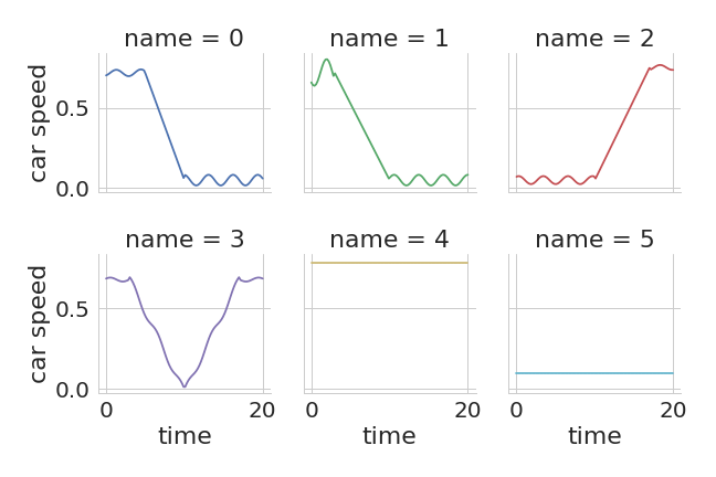
Example:. Most freeways have bottlenecks that lead to traffic congestion, and if there is a stalled or a crashed vehicle(s) at this site, then upstream traffic congestion can severely worsen. For example, Fig 1 shows a series of potential time-series signals to which we would like to assign pairwise distances indicating the similarity (small values) or differences (large values) between any two time series. To ease exposition, we have limited our focus to the car’s speed. In signals 0 and 1, both cars transition from high speed freeway driving to stop and go traffic. Conversely, in signal 2, the car transitions from stop and go traffic to high speed freeway driving. Signal 3 corresponds to a car slowing to a stop and then accelerating, perhaps due to difficulty merging lanes. Finally, signal 4 signifies a car encountering no traffic and signal 5 corresponds to a car in heavy traffic, or a possibly stalled vehicle.

Suppose a user wished to find a feature space equipped with a measure to distinguish cars being stuck in traffic. Some properties might be:

1. Signals 0 and 1 should be very close together since both show a car entering stop and go traffic in nearly the same manner.

2. Signals 2, 3, and 4 should be close together since the car ultimately escapes stop and go traffic.

3. Signal 5 should be far from all other examples since it does not represent entering or leaving stop and go traffic.

(a) Statistical feature space

(b) Trade-off boundaries in specification.

Figure 3: Adjacency matrix and clustering of Fig 1. Smaller numbers mean that the time series are more similar with respect to the logical distance metric.

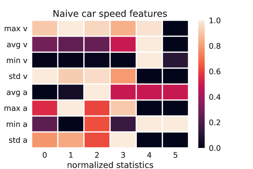
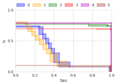
For a strawman comparison, we consider two ways the user might assign a distance measure to the above signal space. Further, we omit generic time series distance measures such as Dynamic Time Warping [8] which do not offer the ability to embed domain specific knowledge into the metric. At first, the user might treat the signals as a series of independent measurements and attempt to characterize the signals via standard statistical measures on the speed and acceleration (mean, standard deviation, etc.). Fig 2(a) illustrates how the example signals look in this feature space with each component normalized between 0 and 1. The user might then use the Euclidean distance of each feature to assign a distance between signals. Unfortunately, in this measure, signal 4 is not close to signal 2 or 3, violating the second desired property. Further, signals 0 and 1 are not “very” close together violating the first property. Next, the user attempts to capture traffic slow downs by the following (informal) parametric temporal specification: “Between time $\tau$ and 20, the car speed is always less than $h$.”. As will be made precise in the preliminaries (for each individual time-series) Fig 2(b) illustrates the boundaries between values of $\tau$ and $h$ that make the specification true and values which make the specification false. The techniques in [16] then require the user to specify a particular total ordering on the parameter space. One then uses the maximal point on the boundary as the representative for the entire boundary. However, in practice, selecting a good ordering a-priori is non-obvious. For example, [16] suggests a lexicographic ordering of the parameters. However, since most of the boundaries start and end at essentially the same point, applying any of the lexicographic orderings to the boundaries seen in Fig 2(b) would result in almost all of the boundaries collapsing to the same points. Thus, such an ordering would make characterizing a slow down impossible.

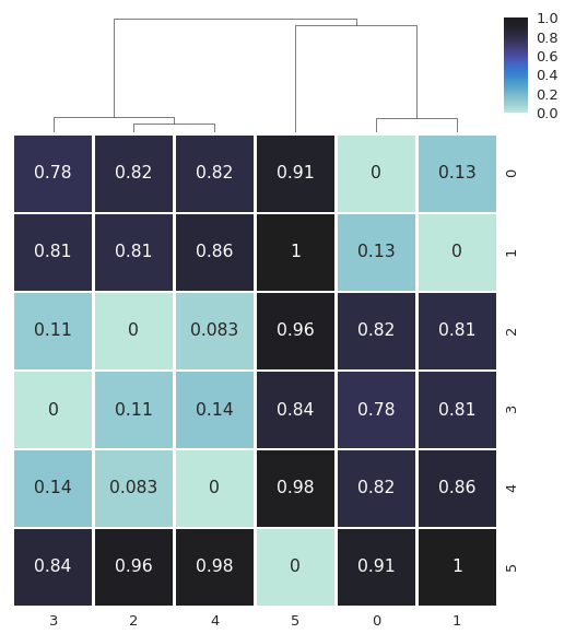
In the sequel, we propose using the Hausdorff distance between boundaries as a general ordering-free way to endow time series with a “logic respecting distance metric”. Fig 3 illustrates the distances between each boundary. As is easily confirmed, all 3 properties desired of the clustering algorithm hold.

Contributions. The key insight in our work is that in many interesting examples, the distance between satisfaction boundaries in the parameter space of parametric logical formula can characterize the domain-specific knowledge implicit in the parametric formula. Leveraging this insight we provide the following contributions:

1. We propose a new distance measure between time-series through the lens of a chosen monotonic specification. Distance measure in hand, standard ML algorithms such as nearest neighbors (supervised) or agglomerative clustering (unsupervised) can be used to glean insights into the data.

2. Given a labeling, we propose a method for computing representative points on each boundary. Viewed another way, we propose a form of dimensionality reduction based on the temporal logic formula.

3. Finally, given the representative points and their labels, we can use the machinery developed in [16] to extract a simple logical formula as a classifier for each label.

2 Preliminaries

The main object of analysis in this paper are time-series.

Definition 1 (Time Series, Signals, Traces)

Let $T$ be a subset of $\mathbb{R}^{\geq 0}$ and $\mathcal{D}$ be a nonempty set. A time series (signal or trace), $\mathbf{x}$ is a map:

$$\mathbf{x}:T\to\mathcal{D}$$ (1)

Where $T$ and $\mathcal{D}$ are called the time domain and value domain respectively. The set of all time series is denoted by $\mathcal{D}^{T}$.

Between any two time series one can define a metric which measures their similarity.

Definition 2 (Metric)

Given a set $X$, a metric is a map,

$$d:X\times X\to\mathbb{R}^{\geq 0}$$ (2)

such that $d(x,y)=d(y,x)$, $d(x,y)=0\iff x=y$, $d(x,z)\leq d(x,y)+d(y,z)$.

Example 1 (Infinity Norm Metric)

The infinity norm induced distance $d_{\infty}(\vec{x},\vec{y})\mathrel{\stackrel{{\scriptstyle\makebox[0.0pt]{\mbox{\tiny def}}}}{{=}}}\max_{i}\left({|x_{i}-y_{i}|}\right)$ is a metric.

Example 2 (Hausdorff Distance)

Given a set $X$ with a distance metric $d$, the Hausdorff distance is a distance metric between closed subsets of $X$. Namely, given closed subsets $A,B\subseteq X$:

$$d_{H}(A,B)\mathrel{\stackrel{{\scriptstyle\makebox[0.0pt]{\mbox{\tiny def}}}}{{=}}}\max\left(\sup_{x\in A}~{}\inf_{y\in B}(d(x,y)),\sup_{y\in B}~{}\inf_{x\in A}(d(y,x))\right)$$ (3)

We use the following property of the Hausdorff distance throughout the paper: Given two sets $A$ and $B$, there necessarily exists points $a\in A$ and $b\in B$ such that:

$$d_{H}(A,B)=d(a,b)$$ (4)

Within a context, the platonic ideal of a metric between traces respects any domain-specific properties that make two elements “similar”. A logical trace property, also called a specification, assigns to each timed trace a truth value.

Definition 3 (Specification)

A specification is a map, $\phi$, from time series to true or false.

$$\phi:\mathcal{D}^{T}\to\{1,0\}$$ (5)

A time series, $\mathbf{x}$, is said to satisfy a specification iff $\phi(\mathbf{x})=1$.

Example 3

Consider the following specification related to the specification from the running example:

$$\phi_{ex}(\mathbf{x})\mathrel{\stackrel{{\scriptstyle\makebox[0.0pt]{\mbox{\tiny def}}}}{{=}}}\mathbbm{1}\bigg{[}\forall t\in T~{}.~{}\big{(}t>0.2\implies\mathbf{x}(t)<1\big{)}\bigg{]}(\mathbf{x})$$ (6)

where $\mathbbm{1}[\cdot]$ denotes an indicator function. Informally, this specification says that after $t=0.2$, the value of the time series, $x(t)$, is always less than 1.

Given a finite number of properties, one can then “fingerprint” a time series as a Boolean feature vector. That is, given $n$ properties, $\phi_{1}\ldots\phi_{n}$ and the corresponding indicator functions, $\phi_{1}\ldots\phi_{n}$, we map each time series to an $n$-tuple as follows.

$$\mathbf{x}\mapsto(\phi_{1}(\mathbf{x}),\ldots,\phi_{n}(\mathbf{x}))$$ (7)

Notice however that many properties are not naturally captured by a finite sequence of binary features. For example, imagine a single quantitative feature $f:\mathcal{D}^{T}\to[0,1]$ encoding the percentage of fuel left in a tank. This feature implicitly encodes an uncountably infinite family of Boolean features $\phi_{k}(\mathbf{x})=\mathbbm{1}[f(\mathbf{x})=k](\mathbf{x})$ indexed by the percentages $k\in[0,1]$. We refer to such families as parametric specifications. For simplicity, we assume that the parameters are a subset of the unit hyper-box.

Definition 4 (Parametric Specifications)

A parametric specification is a map:

$$\varphi:\mathcal{D}^{T}\to\bigg{(}{[0,1]}^{n}\to\{0,1\}\bigg{)}$$ (8)

where $n\in\mathbb{N}$ is the number of parameters and $\bigg{(}{[0,1]}^{n}\to\{0,1\}\bigg{)}$ denotes the set of functions from the hyper-square, ${[0,1]}^{n}$ to $\{0,1\}$.

Remark 1

The signature, $\varphi:{[0,1]}^{n}\to(\mathcal{D}^{T}\to\left\{0,1\right\})$ would have been an alternative and arguably simpler definition of parametric specifications; however, as we shall see, (8) highlights that a trace induces a structure, called the validity domain, embedded in the parameter space.

Parametric specifications arise naturally from syntactically substituting constants with parameters in the description of a specification.

Example 4

The parametric specification given in Ex 3 can be generalized by substituting $\tau$ for $0.2$ and $h$ for $1$ in Ex 3.

$$\varphi_{ex}(\mathbf{x})(\tau,h)\mathrel{\stackrel{{\scriptstyle\makebox[0.0pt]{\mbox{\tiny def}}}}{{=}}}\mathbbm{1}\bigg{[}\forall t\in T~{}.~{}\big{(}t>\tau\implies\mathbf{x}(t)<h\big{)}\bigg{]}(\mathbf{x})$$ (9)

At this point, one could naively extend the notion of the “fingerprint” of a parametric specification in a similar manner as the finite case. However, if ${[0,1]}^{n}$ is equipped with a distance metric, it is fruitful to instead study the geometry induced by the time series in the parameter space. To begin, observe that the value of a Boolean feature vector is exactly determined by which entries map to $1$. Analogously, the set of parameter values for which a parameterized specification maps to true on a given time series acts as the “fingerprint”. We refer to this characterizing set as the validity domain.

Definition 5 (Validity domain)

Given an $n$ parameter specification, $\varphi$, and a trace, $\mathbf{x}$, the validity domain is the pre-image of 1 under $\varphi(\mathbf{x})$,

$$\mathcal{V}_{\varphi}(\mathbf{x})\mathrel{\stackrel{{\scriptstyle\makebox[0.0pt]{\mbox{\tiny def}}}}{{=}}}\text{PreImg}_{\varphi(\mathbf{x})}[1]=\bigg{\{}\theta\in{[0,1]}^{n}~{}|~{}\varphi(\mathbf{x})(\theta)=1\bigg{\}}$$ (10)

Thus, $\mathcal{V}_{\varphi}$, can be viewed as the map that returns the structure in the parameter space indexed by a particular trace.

Note that in general, the validity domain can be arbitrarily complex making reasoning about its geometry intractable. We circumvent such hurdles by specializing to monotonic specifications.

Definition 6 (Monotonic Specifications)

A parametric specification is said to be monotonic if for all traces, $\mathbf{x}$:

$$\theta\trianglelefteq\theta^{\prime}\implies\varphi(\mathbf{x})(\theta)\leq\varphi(\mathbf{x})(\theta^{\prime})$$ (11)

where $\trianglelefteq$ is the standard product ordering on ${[0,1]}^{n}$, e.g. $(x,y)\leq(x^{\prime},y^{\prime})$ iff $(x<x^{\prime}\wedge y<y^{\prime})$.

Remark 2

The parametric specification in Ex 4 is monotonic.

Proposition 1

Given a monotonic specification, $\varphi$, and a time series, $\mathbf{x}$, the boundary of the validity domain, $\partial\mathcal{V}_{\varphi}(x)$, of a monotonic specification is a hyper-surface that segments ${[0,1]}^{n}$ into two components.

In the sequel, we develop a distance metric between validity domains which characterizes the similarity between two time series under the lens of a monotonic specification.

3 Logic-Respecting Distance Metric

In this section, we define a class of metrics on the signal space that is derived from corresponding parametric specifications. First, observe that the validity domains of monotonic specifications are uniquely defined by the hyper-surface that separates them from the rest of the parameter space. Similar to Pareto fronts in a multi-objective optimization, these boundaries encode the trade-offs required in each parameter to make the specification satisfied for a given time series. This suggests a simple procedure to define a distance metric between time series that respects their logical properties: Given a monotonic specification, a set of time series, and a distance metric between validity domain boundaries:

1. Compute the validity domain boundaries for each time series.

2. Compute the distance between the validity domain boundaries.

Of course, the benefits of using this metric would rely entirely on whether (i) The monotonic specification captures the relevant domain-specific details (ii) The distance between validity domain boundaries is sensitive to outliers. While the choice of specification is highly domain-specific, we argue that for many monotonic specifications, the distance metric should be sensitive to outliers as this represents a large deviation from the specification. This sensitivity requirement seems particularly apt if the number of satisfying traces of the specification grows linearly or super-linearly as the parameters increase. Observing that Hausdorff distance (3) between two validity boundaries satisfy these properties, we define our new distance metric between time series as:

Definition 7

Given a monotonic specification, $\varphi$, and a distance metric on the parameter space $({[0,1]}^{n},d)$, the logical distance between two time series, $\mathbf{x}(t),\mathbf{y}(t)\in\mathcal{D}^{T}$ is:

$$d_{\varphi}(\mathbf{x}(t),\mathbf{y}(t))\mathrel{\stackrel{{\scriptstyle\makebox[0.0pt]{\mbox{\tiny def}}}}{{=}}}d_{H}\left(\partial\mathcal{V}_{\varphi}(\mathbf{x}),\partial\mathcal{V}_{\varphi}(\mathbf{y})\right)$$ (12)

3.1 Approximating the Logical Distance

Next, we discuss how to approximate the logical distance metric within arbitrary precision. First, observe that the validity domain boundary of a monotonic specification can be recursively approximated to arbitrary precision via binary search on the diagonal of the parameter space [13]. This approximation yields a series of overlapping axis aligned rectangles that are guaranteed to contain the boundary (see Fig 4).

Figure 4: Illustration of procedure introduced in [13] to recursively approximate a validity domain boundary to arbitrary precision.

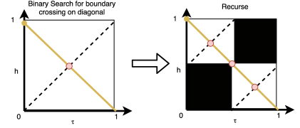
To formalize this approximation, let $I(\mathbb{R})$ denote the set of closed intervals on the real line. We then define an axis aligned rectangle as the product of closed intervals.

Definition 8

The set of axis aligned rectangles is defined as:

$$I(\mathbb{R}^{n})\mathrel{\stackrel{{\scriptstyle\makebox[0.0pt]{\mbox{\tiny def}}}}{{=}}}\prod_{i=1}^{n}I(\mathbb{R})$$ (13)

The approximation given in [13] is then a family of maps,

$$\text{approx}^{i}:\mathcal{D}^{T}\to\mathscr{P}\left(I(\mathbb{R}^{n})\right)$$ (14)

where $i$ denotes the recursive depth $\mathscr{P}\left(\cdot\right)$ denotes the powerset. For example, $\text{approx}^{0}$ yields the bounding box given in the leftmost subfigure in Fig 4 and $\text{approx}^{1}$ yields the subdivision of the bounding box seen on the right.

Next, we ask the question: Given a discretization of the rectangle set approximating a boundary, how does the Hausdorff distance between the discretization relate to the true Hausdorff distance between two boundaries? In particular, consider the map that takes a set of rectangles to the set of the corner points of the rectangles. Formally, we denote this map as:

$$\text{discretize}:\mathscr{P}\left(I(\mathbb{R}^{n})\right)\to\mathscr{P}\left(\mathbb{R}^{n}\right)$$ (15)

As the rectangles are axis aligned, at this point, it is fruitful to specialize to parameter spaces equipped with the infinity norm. The resulting Hausdorff distance is denoted $d_{H}^{\infty}$. This specialization leads to the following lemma:

Lemma 1

Let $\mathbf{x}$, $\mathbf{x}^{\prime}$ be two time series and $\mathcal{R},\mathcal{R}^{\prime}$ the approximation of their respective boundaries. Further, let $p,p^{\prime}$ be points in $\mathcal{R},\mathcal{R}^{\prime}$ such that:

$$\hat{d}\mathrel{\stackrel{{\scriptstyle\makebox[0.0pt]{\mbox{\tiny def}}}}{{=}}}d_{H}^{\infty}(\text{discretize}(\mathcal{R}),\text{discretize}(\mathcal{R^{\prime}}))=d_{\infty}(p,p^{\prime})$$ (16)

and let $r,r^{\prime}$ be the rectangles in $\mathcal{R}$ and $\mathcal{R}^{\prime}$ containing the points $p$ and $p^{\prime}$ respectively. Finally, let $\frac{\epsilon}{2}$ be the maximum edge length in $\mathcal{R}$ and $\mathcal{R^{\prime}}$, then:

$$\max(0,\hat{d}-\epsilon)\leq d_{\varphi}(\mathbf{x},\mathbf{x}^{\prime})\leq\hat{d}+\epsilon$$ (17)

Proof

First, observe that (i) each rectangle intersects its boundary (ii) each rectangle set over-approximates its boundary. Thus, by assumption, each point within a rectangle is at most $\epsilon/2$ distance from the boundary w.r.t. the infinity norm. Thus, since there exist two points $p,p^{\prime}$ such that $\hat{d}=d_{\infty}(p,p^{\prime})$, the maximum deviation from the logical distance is at most $2\frac{\epsilon}{2}=\epsilon$ and $\hat{d}-2\epsilon\leq d_{\varphi}(\mathbf{x},\mathbf{x}^{\prime})\leq\hat{d}+2\epsilon$. Further, since $d_{\varphi}$ must be in $\mathbb{R}^{\geq 0}$, the lower bound can be tightened to $\max(0,\hat{d}-2\epsilon)$. $\blacksquare$

We denote the map given by (17) from the points to the error interval as:

$$d_{H}^{\infty}\pm\epsilon:\mathscr{P}\left(\mathbb{R}\right)\times\mathscr{P}\left(\mathbb{R}\right)\to I(\mathbb{R}^{+})$$ (18)

Next, observe that this approximation can be made arbitrarily close to the logical distance.

Theorem 3.1

Let $d^{\star}=d_{\varphi}(\mathbf{x},\mathbf{y})$ denote the logical distance between two traces $\mathbf{x},\mathbf{y}$. For any $\epsilon\in\mathbb{R}^{\geq 0}$, there exists $i\in\mathbb{N}$ such that:

$$d_{H}^{\infty}(\text{discretize}(\text{approx}^{i}(\mathcal{R})),\text{discretize}(\text{approx}^{i}(\mathcal{R}^{\prime})))\in[d^{\star}-\epsilon,d^{\star}+\epsilon]$$ (19)

Proof

By Lemma 1, given a fixed approximate depth, the above approximation differs from the true logical distance by at most two times the maximum edge length of the approximating rectangles. Note that by construction, incrementing the approximation depth results in each rectangle having at least one edge being halved. Thus the maximum edge length across the set of rectangles must at least halve. Thus, for any $\epsilon$ there exists an approximation depth $i\in\mathbb{N}$ such that:

$$d_{H}^{\infty}(\text{discretize}(\text{approx}^{i}(\mathcal{R})),\text{discretize}(\text{approx}^{i}(\mathcal{R}^{\prime})))\in[d^{\star}-\epsilon,d^{\star}+\epsilon]~{}.~{}\blacksquare$$

Finally, algorithm 1 summarizes the above procedure.

Algorithm 1 Approximate Logical Distance

1:procedure approx_dist($\mathbf{x},\mathbf{x}^{\prime},\delta$)

2:    $lo,hi\leftarrow 0,\infty$

3:    while $hi-lo>\delta$ do

4:       $\mathcal{R},\mathcal{R}^{\prime}\leftarrow\text{approx}^{i}(\mathbf{x}),\text{approx}^{i}(\mathbf{x}^{\prime})$

5:       $\text{points},\text{points}^{\prime}\leftarrow\text{discretize}(\mathcal{R}),\text{discretize}(\mathcal{R}^{\prime})$

6:       $lo,hi\leftarrow\big{(}d_{H}^{\infty}\pm\epsilon\big{)}(\mathcal{R},\mathcal{R}^{\prime})$     

7:    return $lo,hi$

Remark 3

An efficient implementation should of course memoize previous calls to $\text{approx}^{i}$ and use $\text{approx}^{i}$ to compute $\text{approx}^{i+1}$. Further, since certain rectangles can be quickly determined to not contribute to the Hausdorff distance, they need not be subdivided further.

3.2 Learning Labels

The distance interval $(lo,hi)$ returned by Alg 1 can be used by learning techniques, such as hierarchical or agglomerative clustering, to estimate clusters (and hence the labels). While the technical details of these learning algorithms are beyond the scope of this work, we formalize the result of the learning algorithms as a labeling map:

Definition 9 (Labeling)

A $k$-labeling is a map:

$$L:\mathcal{D}^{T}\to\{0,\ldots,k\}$$ (20)

for some $k\in\mathbb{N}$. If $k$ is obvious from context or not important, then the map is simply referred to as a labeling.

4 Artifiact Extraction

In practice, many learning algorithms produce labeling maps that provide little to no insight into why a particular trajectory is given a particular label. In the next section, we seek a way to systematically summarize a labeling in terms of the parametric specification used to induce the logical distance.

4.1 Post-facto Projections

To begin, observe that due to the nature of the Hausdorff distance, when explaining why two boundaries differ, one can remove large segments of the boundaries without changing their Hausdorff distance. This motivates us to find a small summarizing set of parameters for each label. Further, since the Hausdorff distance often reduces to the distance between two points, we aim to summarize each boundary using a particular projection map. Concretely,

Definition 10

Letting $\partial\mathcal{V}_{\varphi}(\mathcal{D}^{T})$ denote the set of all possible validity domain boundaries, a projection is a map:

$$\pi:\partial\mathcal{V}_{\varphi}(\mathcal{D}^{T})\to\mathbb{R}^{n}$$ (21)

where $n$ is the number of parameters in $\varphi$.

Remark 4

In principle, one could extend this to projecting to a finite tuple of points. For simplicity, we do not consider such cases.

Systematic techniques for picking the projection include lexicographic projections and solutions to multi-objective optimizations; however, as seen in the introduction, a-priori choosing the projection scheme is subtle. Instead, we propose performing a post-facto optimization of a collection of projections in order to be maximally representative of the labels. That is, we seek a projection, $\pi^{*}$, that maximally disambiguates between the labels, i.e., maximizes the minimum distance between the clusters. Formally, given a set of traces associated with each label $L_{1},\ldots L_{k}$ we seek:

$$\pi^{*}\in\operatorname*{arg\,max}_{\pi}\min_{i,j\in{k\choose 2}}d_{\infty}(\pi(L_{i}),\pi(L_{j}))$$ (22)

For simplicity, we restrict our focus to projections induced by the intersection of each boundary with a line intersecting the base of the unit box ${[0,1]}^{n}$. Just as in the recursive boundary approximations, due to monotonicity, this intersection point is guaranteed to be unique. Further, this class of projections is in one-one correspondence with the boundary. In particular, for any point $p$ on boundary, there exists exactly one projection that produces $p$. As such, each projection can be indexed by a point in ${[0,1]}^{n-1}$.

This is perhaps unsurprising given that in 2-d, one can index this class by the angle with the $x$-axis and in 3-d on can include the angle from the $z$-axis.

Remark 5

Since we expect clusters of boundaries to be near each other, we also expect their intersection points to be near each other.

Remark 6

For our experiment, we searched for $\pi^{*}$ via a sweep through a discretized indexing of possible angles.

4.2 Label Specifications

Next, observe that given a projection, when studying the infinity norm distance between labels, it suffices to consider only the bounding box of each label in parameter space. Namely, letting $B:\mathscr{P}\left(\mathbb{R}^{n}\right)\to I[\mathbb{R}^{n}]$ denote the map that computes the bounding box of a set of points in $\mathbb{R}^{n}$, for any two labels $i$ and $j$:

$$d_{\infty}(\pi(L_{i}),\pi(L_{j}))=d_{\infty}(B\circ\pi(L_{i}),B\circ\pi(L_{j})).$$ (23)

This motivates using the projection’s bounding box as a surrogate for the cluster. Next, we observe that one can encode the set of trajectories whose boundaries intersect (and thus can project to) a given bounding box as a simple Boolean combination of the specifications corresponding to instantiating $\varphi$ with the parameters of at most $n+1$ corners of the box [16, Lemma 2]. While a detailed exposition is outside the scope of this article, we illustrate with an example.

Example 5

Consider examples 0 and 1 from the introductory example viewed as validity domain boundaries under (9). Suppose that the post-facto projection mapped example 0 to $(1/4,1/2)$ and mapped example 1 to $(0.3,0.51)$. Such a projection is plausibly near the optimal for many classes of projections since none of the other example boundaries (who are in different clusters) are near the boundaries for 0 and 1 at these points. The resulting specification is:

$$\begin{split}\phi&(\mathbf{x})=\varphi_{ex}(\mathbf{x})(1/4,1/2)\wedge\neg\varphi_{ex}(\mathbf{x})(1/4,0.51)\wedge\neg\varphi_{ex}(\mathbf{x})(0.3,1/2)\\ &=\mathbbm{1}\bigg{[}t\in[1/4,0.3]\implies\mathbf{x}(t)\in[1/2,0.51]\wedge t>0.3\implies\mathbf{x}(t)\geq 0.51\bigg{]}\end{split}$$ (24)

4.3 Dimensionality Reduction

Figure 5: Figure of histogram resulting from projecting noisy variations of the traffic slow down example time series onto the diagonal of the unit box.

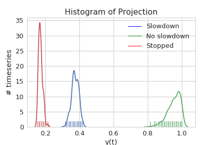
Finally, observe that the line that induces the projection can serve as a mechanism for dimensionality reduction. Namely, if one parameterizes the line $\gamma(t)$ from $[0,1]$, where $\gamma(0)$ is the origin and $\gamma(1)$ intersects the unit box, then the points where the various boundaries intersect can be assigned a number between $0$ and $1$. For high-dimensional parameter spaces, this enables visualizing the projection histogram and could even be used for future classification/learning. We again illustrate using our running example.

Example 6

For all six time series in the traffic slow down example, we generate 100 new time series by modulating the time series with noise drawn from $\mathcal{N}(1,0.3)$. Using our previously labeled time series, the projection using the line with angle $45^{\circ}$ (i.e., the diagonal of the unit box) from the x-axis yields the distribution seen in Fig 5. Observe that all three clusters are clearly visible.

Remark 7

If one dimension is insufficient, this procedure can be extended to an arbitrary number of dimensions using more lines. An interesting extension may be to consider how generic dimensionality techniques such as principle component analysis would act in the limit where one approximates the entire boundary.

5 Case Study

To improve driver models and traffic on highways, the Federal Highway Administration collected detailed traffic data on southbound US-101 freeway, in Los Angeles [4]. Traffic through the segment was monitored and recorded through eight synchronized cameras, next to the freeway. A total of $45$ minutes of traffic data was recorded including vehicle trajectory data providing lane positions of each vehicle within the study area. The data-set is split into $5979$ time series. For simplicity, we constrain our focus to the car’s speed. In the sequel, we outline a technique for first using the parametric specification (in conjunction with off-the-shelf machine learning techniques) to filter the data, and then using the logical distance from an idealized slow down to find the slow downs in the data. This final step offers a key benefit over the closest prior work [16]. Namely given an over approximation of the desired cluster, one can use the logical distance to further refine the cluster.

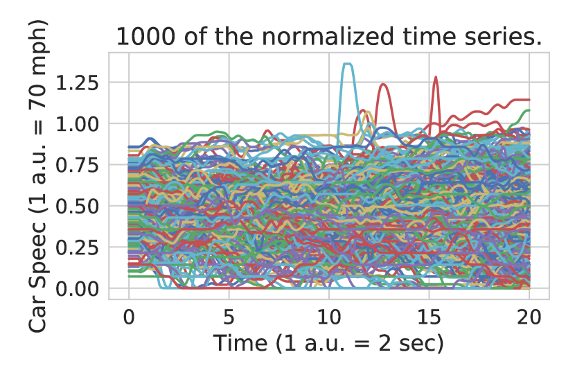
Rescale Data. As in our running example, we seek to use (9) to search for traffic slow downs; however, in order to do so, we must re-scale the time series. To begin, observe that the mean velocity is 62mph with 80% of the vehicles remaining under 70mph. Thus, we linearly scale the velocity so that $70\text{mph}\mapsto 1\text{ arbitrary unit (a.u.)}$. Similarly, we re-scale the time axis so that each tick is $2$ seconds. Fig 6(a) shows a subset of the time series.

(a) 1000 / 5000 of the rescaled highway 101 time series.

(b) Projection of Time-Series to two lines in the parameter space of (9) and resulting GMM labels.

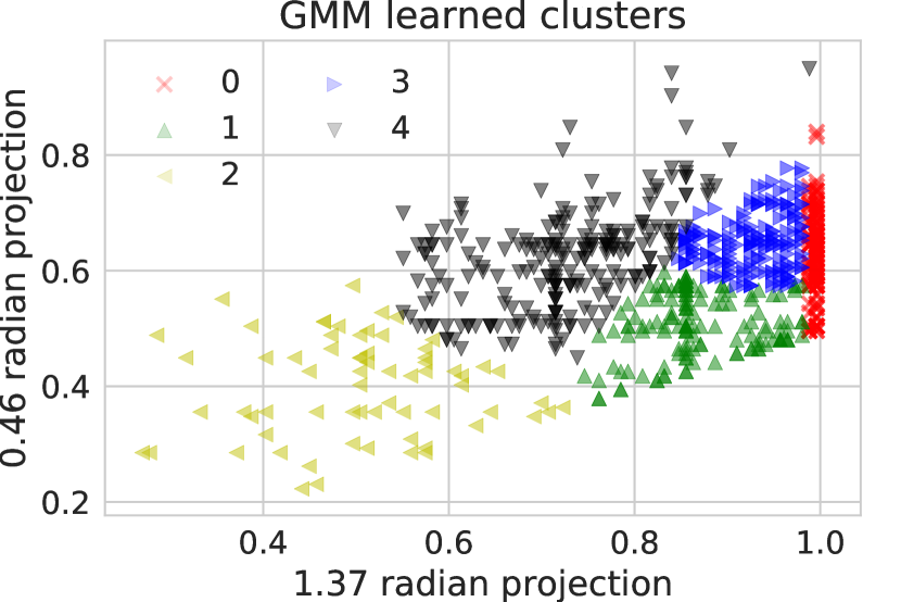
Filtering. Recall that if two boundaries have small Hausdorff distances, then the points where the boundaries intersect a line (that intersects the origin of the parameter space) must be close. Since computing the Hausdorff distance is a fairly expensive operation, we use this one way implication to group time series which may be near each other w.r.t. the Hausdorff distance.

In particular, we (arbitrarily) selected two lines intersecting the parameter space origin at $0.46$ and $1.36$ radians from the $\tau$ axis to project to. We filtered out any time-series that did not intersect the line within ${[0,1]}^{2}$. We then fit a 5 cluster Gaussian Mixture Model (GMM) to label the data. Fig 6(b) shows the result.

(a) Cluster 4 Logical distance histogram.

(b) Time-series in Cluster 4 colored by distance to ideal slow down.

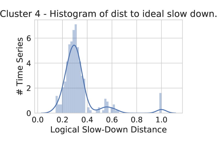
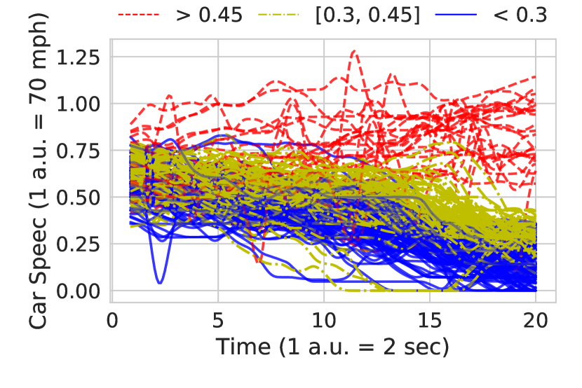
Matching Idealized Slow Down. Next, we labeled the idealized slow down, (trace 0 from Fig 2(b)) using the fitted GMM. This identified cluster 4 (with 765 data points) as containing potential slow downs. To filter for the true slow downs, we used the logical distance from the idealized slow down to further subdivide the cluster. Fig 7(a) shows the resulting distribution. Fig 7(b) shows the time series in cluster 4 annotated by their distance for the idealized slow down. Using this visualization, one can clearly identify 390 slow downs (distance less than $0.3$)

Artifact Extraction. Finally, we first searched for a single projection that gave a satisfactory separation of clusters, but were unable to do so. We then searched over pairs of projections to create a specification as the conjunction of two box specifications. Namely, in terms of $\eqref{eq:param_spec}$, our first projection yields the specification: $\phi_{1}=\varphi_{ex}(0.27,0.55)\wedge\neg\varphi_{ex}(0.38,0.55)\wedge\neg\varphi_{ex}(0.27,0.76)$. Similarly, our second projection yields the specification: $\phi_{2}=\varphi_{ex}(0.35,0.17)\wedge\neg\varphi_{ex}(0.35,0.31)\wedge\neg\varphi_{ex}(0.62,0.17)$. The learned slow down specification is the conjunction of these two specifications.

6 Related Work

Time-series clustering and classification is a well-studied area in the domain of machine learning and data mining [10]. Time series clustering that work with raw time-series data combine clustering schemes such as agglomerative clustering, hierarchical clustering, $k$-means clustering among others, with similarity measures between time-series data such as the dynamic time-warping (DTW) distance, statistical measures and information-theoretic measures. Feature-extraction based methods typically use generic sets of features, but algorithmic selection of the right set of meaningful features is a challenge. Finally, there are model-based approaches that seek an underlying generative model for the time-series data, and typically require extra assumptions on the data such as linearity or the Markovian property. Please see [10] for detailed references to each approach. It should be noted that historically time-series learning focused on univariate time-series, and extensions to multivariate time-series data have been relatively recent developments.

More recent work has focused on automatically identifying features from the data itself, such as the work on shapelets [17, 15, 11], where instead of comparing entire time-series data using similarity measures, algorithms to automatically identify distinguishing motifs in the data have been developed. These motifs or shapelets serve not only as features for ML tasks, but also provide visual feedback to the user explaining why a classification or clustering task, labels given data, in a certain way. While we draw inspiration from this general idea, we seek to expand it to consider logical shapes in the data, which would allow leveraging user’s domain expertise.

Automatic identification of motifs or basis functions from the data while useful in several documented case studies, comes with some limitations. For example, in [1], the authors define a subspace clustering algorithm, where given a set of time-series curves, the algorithm identifies a subspace among the curves such that every curve in the given set can be expressed as a linear combination of a deformations of the curves in the subspace. We note that the authors observe that it may be difficult to associate the natural clustering structure with specific predicates over the data (such as patient outcome in a hospital setting).

The use of logical formulas for learning properties of time-series has slowly been gaining momentum in communities outside of traditional machine learning and data mining [2, 3, 9, 6]. Here, fragments of Signal Temporal Logic have been used to perform tasks such as supervised and unsupervised learning. A key distinction from these approaches is our use of libraries of signal predicates that encode domain expertise that allow human-interpretable clusters and classifiers.

Finally, preliminary exploration of this idea appeared in prior work by some of the co-authors in [16]. The key difference is the previous work required users to provide a ranking of parameters appearing in a signal predicate, in order to project time-series data to unique points in the parameter space. We remove this additional burden on the user in this paper by proposing a generalization that projects time-series signals to trade-off curves in the parameter space, and then using these curves as features.

Conclusion. We proposed a family of distance metrics for time-series learning centered monotonic specifications that respect the logical characteristic of the specification. The key insight was to first map each time-series to characterizing surfaces in the parameter space and then compute the Hausdorff Distance between the surfaces. This enabled embedding non-trivial domain specific knowledge into the distance metric usable by standard machine learning. After labeling the data, we demonstrate how this technique produces artifacts that can be used for dimensionality reduction or as a logical specification for each label. We concluded with a simple automotive case study show casing the technique on real world data. Future work includes investigating how to the leverage massively parallel natural in the boundary and Hausdorff computation using graphical processing units and characterizing alternative boundary distances (see Remark 7).

References

- [1] Bahadori, M.T., Kale, D., Fan, Y., Liu, Y.: Functional Subspace Clustering with Application to Time Series. In: Proc. of ICML. pp. 228–237 (2015)
- [2] Bartocci, E., Bortolussi, L., Sanguinetti, G.: Data-driven statistical learning of temporal logic properties. In: International conference on formal modeling and analysis of timed systems. pp. 23–37. Springer (2014)
- [3] Bombara, G., Vasile, C.I., Penedo, F., Yasuoka, H., Belta, C.: A Decision Tree Approach to Data Classification using Signal Temporal Logic. In: Proc. of HSCC. pp. 1–10 (2016)
- [4] Colyar, J., Halkias, J.: US highway 101 dataset. Federal Highway Administration (FHWA), Tech. Rep. FHWA-HRT-07-030 (2007)
- [5] Deng, D., Shahabi, C., Demiryurek, U., Zhu, L., Yu, R., Liu, Y.: Latent space model for road networks to predict time-varying traffic. In: Proceedings of the 22nd ACM SIGKDD International Conference on Knowledge Discovery and Data Mining. pp. 1525–1534. ACM (2016)
- [6] Jones, A., Kong, Z., Belta, C.: Anomaly detection in cyber-physical systems: A formal methods approach. In: Proc. of CDC. pp. 848–853 (2014)
- [7] Kale, D.C., Gong, D., Che, Z., Liu, Y., Medioni, G., Wetzel, R., Ross, P.: An Examination of Multivariate Time Series Hashing with Applications to Health Care. In: Data Mining (ICDM), 2014 IEEE International Conference on. pp. 260–269. IEEE (2014)
- [8] Keogh, E.J., Pazzani, M.J.: Scaling up dynamic time warping for data mining applications. In: Proc. of KDD. pp. 285–289 (2000)
- [9] Kong, Z., Jones, A., Medina Ayala, A., Aydin Gol, E., Belta, C.: Temporal logic inference for classification and prediction from data. In: Proc. of HSCC. pp. 273–282 (2014)
- [10] Liao, T.W.: Clustering of time series data survey. Pattern recognition 38(11), 1857–1874 (2005)
- [11] Lines, J., Davis, L.M., Hills, J., Bagnall, A.: A shapelet transform for time series classification. In: Proceedings of the 18th ACM SIGKDD international conference on Knowledge discovery and data mining. pp. 289–297. ACM (2012)
- [12] Liu, Y., Bahadori, T., Li, H.: Sparse-gev: Sparse latent space model for multivariate extreme value time series modeling. In: Proc. of ICML (2012)
- [13] Maler, O.: Learning Monotone Partitions of Partially-Ordered Domains (Work in Progress) (Jul 2017), https://hal.archives-ouvertes.fr/hal-01556243, working paper or preprint
- [14] McCall, J.C., Trivedi, M.M.: Driver behavior and situation aware brake assistance for intelligent vehicles. Proceedings of the IEEE 95(2), 374–387 (2007)
- [15] Mueen, A., Keogh, E., Young, N.: Logical-shapelets: an expressive primitive for time series classification. In: Proceedings of the 17th ACM SIGKDD international conference on Knowledge discovery and data mining. pp. 1154–1162. ACM (2011)
- [16] Vazquez-Chanlatte, M., Deshmukh, J.V., Jin, X., Seshia, S.A.: Logic-based clustering and learning for time-series data. In: Proc. International Conference on Computer-Aided Verification (CAV) (2017)
- [17] Ye, L., Keogh, E.: Time series shapelets: a new primitive for data mining. In: In Proc. of the 15th ACM SIGKDD international conference on Knowledge discovery and data mining. pp. 947–956. ACM (2009)