A Semi-Smooth Newton Algorithm for
High-Dimensional Nonconvex Sparse Learning

Abstract

The smoothly clipped absolute deviation (SCAD) and the minimax concave penalty (MCP) penalized regression models are two important and widely used nonconvex sparse learning tools that can handle variable selection and parameter estimation simultaneously, and thus have potential applications in various fields such as mining biological data in high-throughput biomedical studies. Theoretically, these two models enjoy the oracle property even in the high-dimensional settings, where the number of predictors $p$ may be much larger than the number of observations $n$. However, numerically, it is quite challenging to develop fast and stable algorithms due to their non-convexity and non-smoothness. In this paper we develop a fast algorithm for SCAD and MCP penalized learning problems. First, we show that the global minimizers of both models are roots of the nonsmooth equations. Then, a semi-smooth Newton (SSN) algorithm is employed to solve the equations. We prove that the SSN algorithm converges locally and superlinearly to the Karush-Kuhn-Tucker (KKT) points. Computational complexity analysis shows that the cost of the SSN algorithm per iteration is $O(np)$. Combined with the warm-start technique, the SSN algorithm can be very efficient and accurate. Simulation studies and a real data example suggest that our SSN algorithm, with comparable solution accuracy with the coordinate descent (CD) and the difference of convex (DC) proximal Newton algorithms, is more computationally efficient.

I Introduction

This paper introduces a fast algorithm for concavely penalized regression. We focus on the linear regression model

$$y=X\beta^{{\dagger}}+\varepsilon,$$ (1)

where $y\in\mathbb{R}^{n}$ is an $n\times 1$ vector of response variables, $X=(X_{1},\ldots,X_{p})$ is an $n\times p$ design matrix, $\varepsilon$ is an $n\times 1$ vector of error terms, and $\beta^{{\dagger}}=(\beta^{{\dagger}}_{1},\ldots,\beta^{{\dagger}}_{p})^{T}\in\mathbb{R}^{p}$ is the vector of underlying regression coefficients.

Under the sparsity assumption that the number of important predictors is relatively small, it is natural to consider the estimator that solves the minimization problem

$$\min_{\beta\in\mathbb{R}^{p}}\|X\beta-y\|^{2}_{2}\quad\textrm{subject to}\quad\|\beta\|_{0}\leq\tau,$$ (2)

where $\|\beta\|_{0}$ denotes the number of nonzero elements of $\beta$ and $\tau>0$ is a tuning parameter controlling the sparsity level. However, the minimization problem (2) is NP-hard [1], hence it is quite challenging to design a feasible algorithm for solving it when $p$ is large. Replacing the $\|\beta\|_{0}$ term in (2) by $\|\beta\|_{1}$, we get the $\ell_{1}$ penalized problem or the LASSO [2]

$$\min_{\beta\in\mathbb{R}^{p}}\|X\beta-y\|^{2}_{2}\quad\textrm{subject to}\quad\|\beta\|_{1}\leq\tau,$$ (3)

which can be viewed as a convex relaxation of (2). Numerically, it is convenient to consider the Lagrange form of (3)

$$\min_{\beta\in\mathbb{R}^{p}}\frac{1}{2}\|X\beta-y\|^{2}_{2}+\lambda\|\beta\|_{1},$$ (4)

which is known as the basis pursuit denoising (BPDN) in the signal processing literature [3], where $\lambda\geq 0$ is a tuning parameter that controls the sparsity level of solutions. Computationally, (4) is a convex minimization problem, therefore, several fast algorithms have been proposed for computing its global minimizer, such as Homotopy or LARS [4, 5] and CD algorithms [6, 7, 8].

Theoretically, under certain regularity conditions on the design matrix $X$, such as the restricted isometry property [9], the strong irrepresentable condition [10, 11] and the sparsity condition on the regression coefficients, LASSO has attractive estimation and selection properties. However, even under these conditions, the minimizer of (4) still suffers from the so-called LASSO bias, which implies that the LASSO regularized estimator does not have the oracle property. To remedy this problem, [12] proposed using concave penalties that can reduce bias and still yield sparse solutions. This leads to the following minimization problem

$$\min_{\beta\in\mathbb{R}^{p}}\frac{1}{2}\|X\beta-y\|^{2}_{2}+\sum_{i=1}^{p}P(\beta_{i};\lambda,\gamma),$$ (5)

where $P(\cdot;\lambda,\gamma)$ is a concave penalty function. Here $\lambda\geq 0$ is the penalty parameter and $\gamma$ is a given parameter that controls the concavity of the penalty. In this paper, we focus on concave penalties SCAD [12] and MCP [13].

The SCAD penalty is defined as

$$P_{scad}(t;\lambda,\gamma)=\lambda\int_{0}^{t}\min\{1,(\gamma-x/\lambda)_{+}/(\gamma-1)\}dx,\gamma>2,$$ (6)

and the MCP takes the form

$$P_{mcp}(t;\lambda,\gamma)=\lambda\int_{0}^{t}(1-x/(\gamma\lambda))_{+}dx,\gamma>1,$$ (7)

where $x_{+}$ is the nonnegative part of $x$, i.e., $x_{+}=x1_{\{x\geq 0\}}$. It is noteworthy that both penalties converge to the $\ell_{1}$ penalty as $\gamma\to\infty$, and the MCP converges to the hard-thresholding penalty as $\gamma\to 1$. The MCP can be easily understood by considering its derivative,

$$\dot{P}_{mcp}(t;\lambda,\gamma)=\lambda\big{(}1-|t|/(\gamma\lambda)\big{)}_{+}\mbox{sign}(t),$$ (8)

where $\mbox{sign}(t)=-1,0,$ or $1$ if $t<0,=0$, or $>0$. The MCP provides a continuum of penalties with the $\ell_{1}$ penalty at $\gamma=\infty$ and a continuous approximation of the hard-thresholding penalty as $\gamma\to 1$.

Concavely penalized estimators have the asymptotic oracle property under appropriate conditions [12, 13]. However, it is quite challenging to solve (5) with (6) and (7) numerically, since the objective functions to be minimized are both nonconvex and nonsmooth. Several methods have been proposed to deal with this difficulty. The first type of the methods can be viewed as special cases of the MM algorithm [14] or of multi-stage convex relaxation [15], such as local quadratic approximation (LQA) [12] and local linear approximation (LLA) [16]. Such algorithms generate a solution sequence $\{\beta^{k}\}_{k}$ that can guarantee the convergence of the objective function, but the convergence property of the iterated solution sequence $\{\beta^{k}\}_{k}$ is generally unknown. Moreover, the cost per iteration of this type of algorithms is the cost of a LASSO solver. The second type of the methods include coordinate descent (CD) type algorithms [17, 18]. The best convergence result of CD algorithms for minimizing (5) is that any cluster point of $\{\beta^{k}\}_{k}$ must be a stationary point of (6) and (7) [17, 18]. As shown in [17, 18], CD-type algorithms are faster than the first type of algorithms mentioned above, because their cost per iteration is only $O(np)$. However, CD-type algorithms may need a large number of iterations when high accuracy is pursued, since their convergence rates are only sublinear or locally linear [19].

In this paper we develop a local but superlinearly convergent algorithm for minimizing (5) with SCAD and MCP. The main contributions of this paper are threefold. First, we establish that the global minimizers of (5) with SCAD (6) and MCP (7) are roots of the nonsmooth KKT equations. Conversely, we show that any root of the KKT equations is at least a global coordinate-wise minimizer and stationary point of (5). Then we adopt the SSN algorithm [20, 21, 22] to solve the nonsmooth KKT equations. Second, we establish the local superlinear convergence property of SSN. Furthermore, the computational complexity analysis shows that the cost of each iteration in SSN is at most $O(np),$ which is the same as CD algorithms. Hence, for a given $\lambda$ and $\gamma$, the overall cost of using SSN to find a (local) minimizer of (5) is still $O(np)$, since SSN always converges after only a few iterations if it is warm started. Thus SSN is possibly one of the fastest and most accurate algorithms for computing the whole solution path of (5) by running SSN repeatedly at some given $\{\lambda_{t}\}_{t}$ with warm start. Third, we conduct extensive numerical experiments to demonstrate the efficiency and accuracy of SSN, as well as the feasibility of proposed tuning parameter selection rules. The comparison results with a CD and a DC Newton-type algorithm verify the effectiveness of SSN and the tuning parameter selectors.

The remainder of this paper is organized as follows. In Section II, we describe the SSN algorithm. In Section III, we establish the local superlinear convergence to KKT points of SSN and analyze its computational complexity. Implementation details and numerical comparisons on simulated and real data are given in Section IV. We conclude in Section V with some comments and suggestions for future work.

II Semi-smooth Newton algorithm for penalized regression

II-A Notations and Background on Newton Derivative

We first introduce the notations used throughout this paper and describe the concepts and properties of the Newton derivative [20, 21, 23, 22].

For a column vector $\beta=(\beta_{1},\beta_{2},...,\beta_{p})^{T}\in\mathbb{R}^{p}$, denote its $q$-norm by $\|\beta\|_{q}=(\sum_{i=1}^{p}|\beta_{i}|^{q})^{\frac{1}{q}}$, $q\in[1,\infty)$, and denote its $\ell_{0}$- and $\ell_{\infty}$- norm by $\|\beta\|_{0}=|\{i:\beta_{i}\neq 0,1\leq i\leq p\}|$ and $\|\beta\|_{\infty}=\max_{1\leq i\leq p}|\beta_{i}|$, respectively. $X^{\mathrm{T}}$ is the transpose of the feature matrix $X\in\mathbb{R}^{n\times p}$, and $\|X\|$ denotes the operator norm of $X$ induced by the vector 2-norm. The matrix $X$ is assumed to be columnwise normalized, i.e., $\|X_{i}\|_{2}=1$ for $i=1,2,...,p$. 1 or 0 denote a column vector or a matrix with elements all 1 or 0. Define $S=\{1,2,...,p\}$. For any $A\subseteq S$ with cardinality $|A|$, denote $\beta_{A}\in\mathbb{R}^{|A|}$( or $X_{A}\in\mathbb{R}^{|A|\times p})$ as the subvector (or submatrix) whose entries (or columns) are listed in $A$. And $X_{AB}$ denotes submatrix of $X$ whose rows and columns are listed in $A$ and $B$ respectively. $\textrm{supp}(\beta)$ denotes the support of $\beta$, and $\mbox{sign}(z)$ denotes the entry-wise sign of a given vector $z$.

Let $F:\mathbb{R}^{m}\rightarrow\mathbb{R}^{l}$ be a nonlinear map. [20, 21, 23, 22] generalized the classical Newton-Raphson algorithm to find a root of $F(z)=\textbf{0}$, where $F$ is not Fréchet differentiable but only Newton differentiable in the following sense.

Definition 1

$F:\mathbb{R}^{m}\rightarrow\mathbb{R}^{l}$ is called Newton differentiable at $x\in\mathbb{R}^{m}$ if there exists an open neighborhood $N(x)$ and a family of mappings $D:N(x)\rightarrow\mathbb{R}^{l\times m}$ such that

$$\|F(x+h)-F(x)-D(x+h)h\|_{2}=o(\|h\|_{2})\quad\text{for}\quad\|h\|_{2}\longrightarrow 0.$$

The set of mappings $\{D(z):z\in N(x)\}$ denoted by $\nabla_{N}F(x)$ is called the Newton derivative of $F$ at $x$.

It can be easily seen that $\nabla_{N}F(x)$ coincides with the Fréchet derivative at $x$ if $F$ is continuously Fréchet differentiable. Let $F_{i}:\mathbb{R}^{m}\rightarrow\mathbb{R}^{1}$ be Newton differentiable at $x$ with Newton derivative $\nabla_{N}F_{i}(x),$ $i=1,2,...,l$, then $F=(F_{1},F_{2},...,F_{l})^{T}$ is also Newton differentiable at $x$ with Newton derivative

$$\nabla_{N}F(x)=(\nabla_{N}F_{i}(x),\nabla_{N}F_{2}(x),...,\nabla_{N}F_{l}(x))^{T}.$$ (9)

Furthermore, if both $F$ and $H$ are Newton differentiable at $x$ then any linear combination of them is also Newton differentiable at $x$, i.e., for any $\theta,\mu\in\mathbb{R}^{1}$,

$$\nabla_{N}(\theta F+\mu G)(x)=\theta\nabla_{N}F(x)+\mu\nabla_{N}G(x).$$ (10)

Let $H:\mathbb{R}^{s}\rightarrow\mathbb{R}^{l}$ be Newton differentiable with Newton derivative $\nabla_{N}H$. Let $L\in\mathbb{R}^{s\times m}$ and define $F(x)=H(Lx+z)$ for any given $z\in\mathbb{R}^{s}$. Then it is easy to check by definition that the chain rule holds, i.e., $F(x)$ is Newton differentiable at $x$ with Newton derivative

$$\nabla_{N}F(x)=\nabla_{N}H(Lx+z)L.$$ (11)

In Lemma 2, we will give two important thresholding functions that are Newton differentiable but not Fréchet differentiable.

II-B Optimality Conditions and Semi-smooth Newton Algorithm

In this subsection, we give a necessary condition for the global minimizers of (5) with the SCAD (6) or the MCP (7) penalty. Specifically, we show that the global minimizers satisfy a set of KKT equations, which are nonsmooth but are Newton differentiable. Then we apply the semi-smooth Newton algorithm to solve these equations.

Now we derive the optimality conditions of the minimizers of (5), with the penalty function $P(z;\lambda,\gamma)$ being $P_{scad}(z;\lambda,\gamma)$ or $P_{mcp}(z;\lambda,\gamma)$.

For a given $t\in\mathbb{R}^{1}$, let

$$T(t;\lambda,\gamma)=\mathop{\mathrm{arg\,min}}\limits_{z\in\mathbb{R}^{1}}\frac{1}{2}(z-t)^{2}+P(z;\lambda,\gamma)$$ (12)

be the thresholding functions corresponding to $P(z;\lambda,\gamma)$, which have closed forms for both SCAD and MCP penalties [17, 18].

Lemma 1

Let $T(t;\lambda,\gamma)$ be defined in (12). Then for $P_{mcp}(z;\lambda,\gamma)$ and $P_{scad}(z;\lambda,\gamma)$, it follows that

$$T_{mcp}(t;\lambda,\gamma)=\left\{\begin{aligned} &\frac{\mathcal{S}(t;\lambda)}{1-1/\gamma},\quad if\quad|t|\leq\gamma\lambda,\\ &t,\qquad\quad\quad if\quad|t|>\gamma\lambda.\end{aligned}\right.$$ (13)

and

$$T_{scad}(t;\lambda,\gamma)=\left\{\begin{aligned} &\mathcal{S}(t;\lambda),&\quad if\quad|t|\leq 2\lambda,\\ &\frac{\mathcal{S}(t;\lambda\gamma/(\gamma-1))}{1-1/(\gamma-1)},&\quad if\quad 2\lambda<|t|\leq\gamma\lambda,\\ &t,&\quad if\quad|t|>\gamma\lambda.\end{aligned}\right.$$ (14)

respectively, where the scalar function $\mathcal{S}(t;\lambda)=\max\{|t|-\lambda,0\}\mbox{sign}(t)$ is the soft-thresholding function [24].

Proof:

See Appendix A. ∎

The following result derives the (nonsmooth) KKT equations for the global minimizers of (5). This result is the basis of the SSN algorithm.

Theorem 1

Let $\widehat{\beta}$ be a global minimizer of (5). Then there exists $\widehat{d}\in\mathbb{R}^{p}$ such that the following optimality conditions hold:

$$\widehat{d} = \widetilde{y}-G\widehat{\beta},$$ (15)

$$\widehat{\beta} = \mathbb{T}(\widehat{\beta}+\widehat{d};\lambda,\gamma),$$ (16)

where $G=X^{T}X,$ $\widetilde{y}=X^{T}y$, and $\mathbb{T}(z;\lambda,\gamma)$ is the component-wise thresholding operator of (12) for a given vector $z\in\mathbb{R}^{p}$. Conversely, if there exists $(\widehat{\beta},\widehat{d})$ satisfying (15) and (16), then $\widehat{\beta}$ is a stationary point of (5).

Proof:

See Appendix B. ∎

Let

$$F(\beta;d)=\begin{bmatrix}F_{1}(\beta;d)\\ F_{2}(\beta;d)\\ \end{bmatrix}:\mathbb{R}^{p}\times\mathbb{R}^{p}\to\mathbb{R}^{2p},$$ (17)

where $F_{1}(\beta;d):=\beta-\mathbb{T}(\widehat{\beta}+\widehat{d};\lambda,\gamma),$ and $F_{2}(\beta;d):=G\beta+d-\widetilde{y}.$ For simplicity, we refer to $F$ as a KKT function. By Theorem 1, the global minimizers of (5) are roots of $F(\beta;d)$. These roots are the stationary points of (5). The thresholding operators corresponding to concave penalties including SCAD and MCP are not differentiable, which in turn results in the non-differentiability of $F$. This makes it difficult to find the roots of $F$. So we resort to the SSN method [20, 21, 23, 22].

Let $z=(\beta;d)$. At the $k$th iteration, the SSN method for finding the roots of $F(z)=0$ consists of two steps.

1. Solve $H^{k}\delta^{k}=-F(z^{k})$ for $\delta^{k}$, where $H^{k}$ is an element of $\nabla_{N}F(z^{k})$.

2. Update $z^{k+1}=z^{k}+\delta^{k}$, set $k\leftarrow k+1$ and go to step (1).

This has the same form as the classical Newton method, except that here we use an element of $\nabla_{N}F(z^{k})$ in step (1). Indeed, the key to the success of this method is to find a suitable and invertible $H^{k}$. We describe the pseudocode for the SSN method in Algorithm 1.

Algorithm 1 SSN for finding a root $z^{*}$ of $F(z)$

1:  Input: initial guess $z^{0}$. Set $k=0$.

2:  for $k=0,1,2,3,\cdots$ do

3:     Choose $H^{k}\in\nabla_{N}F(z^{k})$.

4:     Get the semi-smooth Newton direction $\delta^{k}$ by solving

$$H^{k}\delta^{k}=-F(z^{k}).$$ (18)

5:     Update $z^{k+1}=z^{k}+\delta^{k}$.

6:     Stop or $k:=k+1$. Denote the last iteration by $\widehat{z}$.

7:  end for

8:  Output: $\widehat{z}$ as a estimation of $z^{*}$.

II-C The Newton Derivatives of the KKT Functions

Denote the KKT functions as defined in (17) by $F_{scad}$ and $F_{mcp}$ for SCAD and MCP, respectively. To compute the roots of $F_{mcp}$ and $F_{scad}$ based on the SSN method, we need to calculate their Newton derivatives.

Lemma 2

${T}_{mcp}(t;\lambda,\gamma)$ and ${T}_{scad}(t;\lambda,\gamma)$ are Newton differentiable with respect to $t$ with Newton derivatives

$$\nabla_{N}{T}_{mcp}(t)=\left\{\begin{array}[]{ll}$ 0$,&\text{$|t|<\lambda$,}\\ $\text{$r$ }$\in\mathbb{R}^{1},&\text{$|t|=\lambda$,}\\ $ 1/(1-1/$\gamma$)$,&\text{$\lambda<|t|<\gamma\lambda$,}\\ $\text{$r$ }$\in\mathbb{R}^{1},&\text{$|t|=\gamma\lambda$,}\\ $ 1$,&\text{$\gamma\lambda<|t|$.}\\ \end{array}\right.$$ (19)

and

$$\nabla_{N}{T}_{scad}(t)=\left\{\begin{array}[]{ll}$ 0$,&\text{$|t|<\lambda$,}\\ $\text{$r$ }$\in\mathbb{R}^{1},&\text{$|t|=\lambda$,}\\ $ \text{1}$,&\text{$\lambda<|t|<2\lambda$,}\\ $\text{$r$ }$\in\mathbb{R}^{1},&\text{$|t|=2\lambda$,}\\ $ \text{1/(1-1/($\gamma$-1))}$,&\text{$2\lambda<|t|<\gamma\lambda$,}\\ $\text{$r$ }$\in\mathbb{R}^{1},&\text{$|t|=\gamma\lambda$,}\\ $ 1 $,&\text{$\gamma\lambda<|t|$.}\end{array}\right.$$ (20)

respectively.

Proof:

See Appendix C. ∎

II-C1 The Newton derivative of $F_{mcp}$

Consider the KKT function $F_{mcp}$. For any given point $z^{k}=(\beta^{k};d^{k})\in\mathbb{R}^{2p}$, define

$$A^{1}_{k} = \{i\in S:\lambda<|\beta^{k}_{i}+d^{k}_{i}|<\lambda\gamma\},$$ (21)

$$A^{2}_{k} = \{i\in S:|\beta^{k}_{i}+d^{k}_{i}|\geq\lambda\gamma\},$$ (22)

$$A_{k} = A^{1}_{k}\cup A^{2}_{k},$$ (23)

$$B_{k} = \{i\in S:|\beta^{k}_{i}+d^{k}_{i}|\leq\lambda\}.$$ (24)

We rearrange the order of the entries of $z^{k}$ as follows:

$$z_{mcp}^{k}=(\beta^{k}_{A^{1}_{k}};d^{k}_{A^{2}_{k}};\beta^{k}_{B_{k}};d^{k}_{A^{1}_{k}};\beta^{k}_{A^{2}_{k}};d^{k}_{B_{k}}).$$

Denote the Newton derivative of $F_{mcp}$ at $z_{mcp}^{k}$ as $\nabla_{N}F_{mcp}(z_{mcp}^{k})$. In Theorem 2, we will show that $H^{k}_{mcp}\in\nabla_{N}F_{mcp}(z_{mcp}^{k})$, where $H^{k}_{mcp}\in\mathbb{R}^{p\times p}$ is given by

$$H^{k}_{mcp}=\begin{bmatrix}H_{11}^{k}&H_{12}^{k}\\ H_{21}^{k}&H_{22}^{k}\\ \end{bmatrix}$$ (25)

with

$$H_{11}^{k} =\begin{bmatrix}-\frac{1}{\gamma-1}I_{A^{1}_{k}A^{1}_{k}}&\textbf{0}&\textbf{0}\\ \textbf{0}&-I_{A^{2}_{k}A^{2}_{k}}&\textbf{0}\\ \textbf{0}&\textbf{0}&I_{B_{k}B_{k}}\\ \end{bmatrix},$$

$$H_{12}^{k} =\begin{bmatrix}-\frac{\gamma}{\gamma-1}I_{A^{1}_{k}A^{1}_{k}}&\textbf{0}&\textbf{0}\\ \textbf{0}&\textbf{0}&\textbf{0}\\ \textbf{0}&\textbf{0}&\textbf{0}\\ \end{bmatrix},$$

$$H_{21}^{k} =\begin{bmatrix}G_{A^{1}_{k}A^{1}_{k}}&\textbf{0}&G_{A^{1}_{k}B_{k}}\\ G_{A^{2}_{k}A^{1}_{k}}&I_{A^{2}_{k}A^{2}_{k}}&G_{A^{2}_{k}B_{k}}\\ G_{B_{k}A^{1}_{k}}&\textbf{0}&G_{B_{k}B_{k}}\\ \end{bmatrix},$$

$$H_{22}^{k} =\begin{bmatrix}I_{A^{1}_{k}A^{1}_{k}}&G_{A^{1}_{k}A^{2}_{k}}&\textbf{0}\\ \textbf{0}&G_{A^{2}_{k}A^{2}_{k}}&\textbf{0}\\ \textbf{0}&G_{B_{k}A^{2}_{k}}&I_{B_{k}B_{k}}\\ \end{bmatrix}.$$

II-C2 The Newton derivative of $F_{scad}$

Now consider the KKT function $F_{scad}$. For any given point $z^{k}=(\beta^{k};d^{k})\in\mathbb{R}^{2p}$, define

$$A^{1}_{k} = \{i\in S:\lambda<|\beta^{k}_{i}+d^{k}_{i}|<2\lambda\},$$ (26)

$$A^{2}_{k} = \{i\in S:2\lambda\leq|\beta^{k}_{i}+d^{k}_{i}|<\lambda\gamma\},$$ (27)

$$A^{3}_{k} = \{i\in S:|\beta^{k}_{i}+d^{k}_{i}|\geq\lambda\gamma\},$$ (28)

$$A^{k} = A^{1}_{k}\cup A^{2}_{k}\cup A^{3}_{k},$$ (29)

$$B_{k} = \{i\in S:|\beta^{k}_{i}+d^{k}_{i}|\leq\lambda\}.$$ (30)

We rearrange the entries of $z_{scad}$ as follows:

$$z_{scad}^{k}=(\beta^{k}_{B_{k}};d^{k}_{A^{1}_{k}};\beta^{k}_{A^{2}_{k}};d^{k}_{A^{3}_{k}};d^{k}_{B_{k}};\beta^{k}_{A^{1}_{k}};d^{k}_{A^{2}_{k}};\beta^{k}_{A^{3}_{k}}).$$

Denote the Newton derivative of $F_{scad}$ at $z_{scad}^{k}$ as $\nabla_{N}F_{scad}(z_{scad}^{k})$. In Theorem 2, we will show that $H^{k}_{scad}\in\nabla_{N}F_{scad}(z_{scad}^{k})$, where $H^{k}_{scad}\in\mathbb{R}^{p\times p}$ is given by

$$H^{k}_{scad}:=\begin{bmatrix}H_{11}^{k}&H_{12}^{k}\\ H_{21}^{k}&H_{22}^{k}\\ \end{bmatrix}$$ (31)

with

$$H_{11}^{k} =\begin{bmatrix}I_{B_{k}B_{k}}&\textbf{0}&\textbf{0}&\textbf{0}\\ \textbf{0}&-I_{A^{1}_{k}A^{1}_{k}}&\textbf{0}&\textbf{0}\\ \textbf{0}&\textbf{0}&-\frac{1}{\gamma-2}I_{A^{2}_{k}A^{2}_{k}}&\textbf{0}\\ \textbf{0}&\textbf{0}&\textbf{0}&-I_{A^{3}_{k}A^{3}_{k}}\\ \end{bmatrix},$$

$$H_{12}^{k} =\begin{bmatrix}\textbf{0}&\textbf{0}&\textbf{0}&\textbf{0}\\ \textbf{0}&\textbf{0}&\textbf{0}&\textbf{0}\\ \textbf{0}&\textbf{0}&-\frac{\gamma-1}{\gamma-2}I_{A^{2}_{k}A^{2}_{k}}&\textbf{0}\\ \textbf{0}&\textbf{0}&\textbf{0}&\textbf{0}\\ \end{bmatrix},$$

$$H_{21}^{k} =\begin{bmatrix}G_{B_{k}B_{k}}&\textbf{0}&G_{B_{k}A^{k}_{2}}&\textbf{0}\\ G_{A^{1}_{k}B_{k}}&I_{A^{1}_{k}A^{1}_{k}}&G_{A^{k}_{1}A^{k}_{1}}&\textbf{0}\\ G_{A^{2}_{k}B_{k}}&\textbf{0}&G_{A^{2}_{k}A^{2}_{k}}&\textbf{0}\\ G_{A^{3}_{k}B_{k}}&\textbf{0}&G_{A^{3}_{k}A^{2}_{k}}&I_{A^{3}_{k}A^{3}_{k}}\\ \end{bmatrix},$$

$$H_{22}^{k} =\begin{bmatrix}I_{B_{k}B_{k}}&G_{B_{k}A^{1}_{k}}&\textbf{0}&G_{B_{k}A^{3}_{k}}\\ \textbf{0}&G_{A^{1}_{k}A^{1}_{k}}&\textbf{0}&G_{A^{1}_{k}A^{3}_{k}}\\ \textbf{0}&G_{A^{2}_{k}A^{1}_{k}}&I_{A^{2}_{k}A^{2}_{k}}&G_{A^{2}_{k}A^{3}_{k}}\\ \textbf{0}&G_{A^{3}_{k}A^{1}_{k}}&\textbf{0}&G_{A^{3}_{k}A^{3}_{k}}\\ \end{bmatrix}.$$

Theorem 2

Both $F_{mcp}$ and $F_{scad}$ are Newton differentiable at $z_{mcp}^{k}$ and $z_{scad}^{k}$ with

$$H_{mcp}^{k}\in\nabla_{N}F_{mcp}(z_{mcp}^{k}),$$

and

$$H_{scad}^{k}\in\nabla_{N}F_{scad}(z_{scad}^{k}),$$

respectively. Furthermore, the inverses of $H_{mcp}^{k}$ and $H_{scad}^{k}$ are uniformly bounded with

$$\|(H_{mcp}^{k})^{-1}\|\leq M_{\gamma}$$

and

$$\|(H_{scad}^{k})^{-1}\|\leq M_{\gamma},$$

where $M_{\gamma}=(3\gamma+2)+(\gamma+1)(2\gamma+5)$.

Proof:

See Appendix D. ∎

With the Newton derivatives at hand we can apply SSN to compute the roots of $F_{mcp}$ and $F_{scad}$. We first give the details for $F_{mcp}$. By the definitions of $A_{k}^{1},A_{k}^{2},I_{k}$ and $T_{mcp}$, we have

$$F_{mcp}(z_{mcp}^{k})=\begin{bmatrix}\beta^{k}_{A_{k}^{1}}-\frac{\gamma}{\gamma-1}(\beta^{k}_{A_{k}^{1}}+d^{k}_{A_{k}^{1}}-\lambda\mbox{sign}(\beta^{k}_{A_{k}^{1}}+d^{k}_{A_{k}^{1}}))\\ \beta^{k}_{A_{k}^{2}}-(\beta^{k}_{A_{k}^{2}}+d^{k}_{A_{k}^{2}})\\ \beta^{k}_{B_{k}}\\ G_{A^{k}_{1}A^{k}_{1}}\beta^{k}_{A^{k}_{1}}+G_{A^{k}_{1}A^{k}_{2}}\beta^{k}_{A^{2}_{k}}+G_{A^{k}_{1}B_{k}}\beta^{k}_{B_{k}}+d^{k}_{A^{1}_{k}}-\widetilde{y}_{A^{1}_{k}}\\ G_{A^{2}_{k}A^{1}_{k}}\beta^{k}_{A^{1}_{k}}+G_{A^{2}_{k}A^{2}_{k}}\beta^{k}_{A^{2}_{k}}+G_{A^{2}_{k}B_{k}}\beta^{k}_{B_{k}}+d^{k}_{A^{2}_{k}}-\widetilde{y}_{A^{2}_{k}}\\ G_{B_{k}A_{k}^{1}}\beta^{k}_{A^{1}_{k}}+G_{B_{k}A_{k}^{2}}\beta^{k}_{A^{2}_{k}}+G_{B_{k}B_{k}}\beta^{k}_{B_{k}}+d^{k}_{B_{k}}-\widetilde{y}_{B_{k}}\end{bmatrix}.$$ (32)

Substituting (32) and (25) into the SSN direction equation

$$H^{k}_{mcp}\delta_{mcp}^{k}=-F_{mcp}(z^{k}_{mcp})$$

and noting that

$$z_{mcp}^{k+1}=z_{mcp}^{k}+\delta_{mcp}^{k},$$

we get (after some tedious algebra)

$$d^{k+1}_{A^{2}_{k}} =\textbf{0},$$ (33)

$$\beta^{k+1}_{B_{k}} =\textbf{0},$$ (34)

$$\widetilde{G}_{A_{k}A_{k}}\beta^{k+1}_{A_{k}} =s_{A_{k}},$$ (35)

$$d_{A^{1}_{k}}^{k+1} =-\beta^{k+1}_{A_{k}^{1}}/\gamma+s_{A_{k}^{1}},$$ (36)

$$d_{B_{k}}^{k+1} =\widetilde{y}_{B_{k}}-G_{B_{k}A_{k}}\beta_{A_{k}}^{k+1},$$ (37)

where

$$\widetilde{G}_{A_{k}A_{k}} = G_{A_{k}A_{k}}-\begin{bmatrix}I_{A^{1}_{k}A^{1}_{k}}/\gamma&\textbf{0}\\ \textbf{0}&\textbf{0}\\ \end{bmatrix},$$ (38)

$$s_{A_{k}^{1}} = \lambda\mbox{sign}(\beta^{k}_{A^{1}_{k}}+d^{k}_{A^{1}_{k}}),$$ (39)

$$s_{A_{k}} = \widetilde{y}_{A_{k}}-\begin{bmatrix}s_{A_{k}^{1}}\\ \textbf{0}\\ \end{bmatrix}.$$ (40)

Then we summarize the above calculation in the following algorithm.

Algorithm 2 SSN for finding a root of $F_{mcp}$

1:  Input: $X,y,\lambda,\gamma$, initial guess $(\beta^{0};d^{0})$. Set $k=0$.

2:  Pre-compute $\widetilde{y}=X^{T}y$ and store it.

3:  for $k=0,1,2,3,\cdots$ do

4:     Compute $A^{1}_{k},A^{2}_{k},A_{k},B_{k}$ by (21) - (24).

5:     $\beta^{k+1}_{B_{k}}=\textbf{0}.$

6:     $d^{k+1}_{A^{2}_{k}}=\textbf{0}$.

7:     Compute $\widetilde{G}_{A_{k}A_{k}},s_{A_{k}^{1}},s_{A_{k}}$ by (38)-(40).

8:     $\beta^{k+1}_{A_{k}}=\widetilde{G}_{A_{k}A_{k}}^{-1}s_{A_{k}}.$

9:     $d_{A^{1}_{k}}^{k+1}=-\beta^{k+1}_{A_{k}^{1}}/\gamma+s_{A_{k}^{1}}$.

10:     $d_{B_{k}}^{k+1}=\widetilde{y}_{B_{k}}-G_{B_{k}A_{k}}\beta_{A_{k}}^{k+1}.$

11:     Check Stop conditionIf stopDenote the last iteration by $\beta_{\widehat{A}},\beta_{\widehat{B}},d_{\widehat{A}},d_{\widehat{B}}.$Else$k:=k+1.$

12:  end for

13:  Output: $\widehat{\beta}=(\beta_{\widehat{A}};\beta_{\widehat{B}})$, $\widehat{d}=(d_{\widehat{A}};d_{\widehat{B}})$.

Next, we derive the SSN algorithm for $F_{scad}$ in a similar fashion. Let

$$\widetilde{G}_{A_{k}A_{k}} = {G}_{A_{k}A_{k}}-\begin{bmatrix}\textbf{0}&\textbf{0}&\textbf{0}\\ \textbf{0}&I_{A^{2}_{k}A^{2}_{k}}/(\gamma-1)&\textbf{0}\\ \textbf{0}&\textbf{0}&\textbf{0}\\ \end{bmatrix},$$ (41)

$$s_{A_{k}^{2}} = \frac{\gamma\lambda}{\gamma-1}\mbox{sign}(\beta^{k}_{A^{2}_{k}}+d^{k}_{A^{2}_{k}}),$$ (42)

$$s_{A_{k}} = \widetilde{y}_{A_{k}}-\begin{bmatrix}d^{k+1}_{A^{1}_{k}}\\ s_{A_{k}^{2}}\\ \textbf{0}\\ \end{bmatrix}.$$ (43)

Then the algorithm for solving $F_{scad}(z)=0$ is as follows.

Algorithm 3 SSN for finding a root of $F_{scad}$

1:  Input: $X,y,\lambda,\gamma$, initial guess $(\beta^{0};d^{0})$. Set $k=0$.

2:  Pre-compute $\widetilde{y}=X^{T}y$ and store it.

3:  for $k=0,1,2,3,\cdots$ do

4:     Compute $A^{1}_{k},A^{2}_{k},A^{3}_{k},A_{k},B_{k}$ by (26) - (30).

5:     $\beta^{k+1}_{B_{k}}=\textbf{0}.$

6:     $d^{k+1}_{A^{1}_{k}}=\lambda\mbox{sign}(\beta^{k}_{A^{1}_{k}}+d^{k}_{A^{1}_{k}}).$

7:     $d^{k+1}_{A^{3}_{k}}=\textbf{0}$.

8:     Compute $\widetilde{G}_{A_{k}A_{k}},s_{A_{k}^{2}},s_{A_{k}}$ by (41)-(43).

9:     $\beta^{k+1}_{A_{k}}=\widetilde{G}_{A_{k}A_{k}}^{-1}s_{A_{k}}.$

10:     $d_{A^{2}_{k}}^{k+1}=-\beta^{k+1}_{A_{k}^{2}}/(\gamma-1)+s_{A_{k}^{2}}$.

11:     $d_{B_{k}}^{k+1}=\widetilde{y}_{B_{k}}-G_{B_{k}A_{k}}\beta_{A_{k}}^{k+1}.$

12:     Check Stop conditionIf stopDenote the last iteration by $\beta_{\widehat{A}},\beta_{\widehat{B}},d_{\widehat{A}},d_{\widehat{B}}.$Else$k:=k+1.$

13:  end for

14:  Output: $\widehat{\beta}=(\beta_{\widehat{A}};\beta_{\widehat{B}})$, $\widehat{d}=(d_{\widehat{A}};d_{\widehat{B}})$.

A natural stopping criterion for both algorithms is when $A_{k}=A_{k+1}$ for some $k$, which can be checked inexpensively. We also stop the algorithms when the number of iterations exceeds some given positive integer $J$ as a safeguard.

Remark 1

Here we give some remarks on the requirements for the design matrix $X$ and the sparsity level of $\beta^{{\dagger}}$. It is obvious that Algorithm 2 and Algorithm 3 are well-defined if $\widetilde{G}_{A_{k}A_{k}}$ in (38) and (41) are invertible. Sufficient conditions to guarantee these are

$$\kappa_{-}(|A_{k}|)>1/\gamma$$ (44)

and

$$\kappa_{-}(|A_{k}|)>1/(\gamma-1),$$ (45)

respectively, where

$$\kappa_{-}(|A_{k}|)=\min_{\|z\|=1,\|z\|_{0}\leq|A_{k}|}\|Xz\|^{2}$$

denotes the smallest sparse eigenvalues of $X$ with order $|A_{k}|$ [25]. Therefore, we need the assumption that the smallest singular value of the submatrixes of $X_{A_{k}}$ bound away from $1/\gamma$ (or $1/(\gamma-1)$) to guarantee the well-posedness of the proposed algorithm. This assumption is reasonable since the size of the active set $A_{k}$ is small, due to the fact that the underlying sparsity level $\|\beta^{{\dagger}}\|_{0}$ is much smaller than the sample size $n$.

III Convergence, complexity analysis and solution path

In this subsection, following [20, 21, 23, 22], we establish the local superlinear convergence to KKT points of Algorithms 2 and 3, and analyze their computational complexity. We also compare the proposed algorithm with some existing related methods.

III-A Convergence Analysis

Theorem 3

Let $\beta_{mcp}^{k}$ and $\beta_{scad}^{k}$ be generated by Algorithms 2 and 3, respectively. Then, $\beta_{mcp}^{k}$ and $\beta_{scad}^{k}$ converge locally and superlinearly to points satisfying equation (15) - (16).

Proof:

See Appendix E. ∎

Remark 2

By Theorem 1 we can see that Algorithms 2 and 3 also converge locally and superlinearly to the stationary points of (5) with MCP (7) and SCAD (6), respectively.

III-B Computational Complexity

We now consider the number of floating point operations per iteration. It takes $O(p)$ flops to finish steps 4-7 (steps 4-8) in Algorithm 2 (Algorithm 3). For step 8 (step 9) in Algorithm 2 (Algorithm 3), inverting the positive definite matrix $\widetilde{G}_{A_{k}A_{k}}$ by Cholesky factorization takes $O(|A_{k}|^{3})$ flops. As for steps 9-10 (steps 10-11) in Algorithm 2 (Algorithm 3), $O(np)$ flops are enough to finish the matrix-vector multiplication. So the overall cost per iteration for Algorithms 2 and Algorithm 3 is $O(\max(|A_{k}|^{3},pn)$. Numerically $|A_{k}|$ usually increases and converges to $O(\|\beta^{{\dagger}}\|_{0})$ if the algorithm is warm started. Therefore, if the underlying solution is sufficiently sparse such that $\|\beta^{{\dagger}}\|_{0}^{3}\leq O(np)$, then it takes $O(np)$ flops per iteration for both algorithms. Hence the overall cost of Algorithms 2 and 3 are still $O(np)$ due to their superlinear convergence. The computational complexity analysis shows that Algorithms 2 and 3 are fast to compute the solution paths with warm start. This is supported by the numerical results presented in Section IV.

The computational cost of CD algorithms [17, 18] or iterative thresholding algorithms [26] for (6) and (7) is also $O(np)$ per iteration. The cluster points of the sequences generated by CD or iterative thresholding also satisfy (15)-(16). But the convergence rates of these two types of algorithms are at best sublinear even in the case of LASSO penalized problem where the object function is convex [27]. Hence it is not surprising that Algorithms 2 and 3 outperform CD-type algorithms in efficiency in our numerical examples given in Section IV.

III-C Solution Path

An important issue in implementing a Newton-type algorithm is how to choose good initial values. We use warm start to determine the initial values. This strategy has been successfully used for computing the LASSO and the Enet paths [7]. It is also a simple but powerful tool to handle the local convergence of concavely penalized regression problems [17, 18, 28]. The local superlinear convergence results in Theorem 3 guarantee that after a small number of iterations we will get an approximate solution with high accuracy if the algorithms are warm started.

We are interested in the whole solution path $\widehat{\beta}(\lambda)$ for $\lambda\in[\lambda_{\min},\lambda_{\max}]$, where $0<\lambda_{\min}<\lambda_{\max}$ are two prespecified numbers. This will be needed for selecting the $\lambda$ values based on a data driven procedure such as cross validation or Bayesian information criterion. Here we approximate the solution path by computing $\widehat{\beta}(\lambda)$ on a given finite grid $\Lambda=\{\lambda_{0},\lambda_{1}...,\lambda_{M}\}$ for some positive integer $M$, where $\lambda_{0}>\lambda_{1}>\ldots>\lambda_{M}>0$. Obviously, $\widehat{\beta}(\lambda)=\textbf{0}$ satisfies (15) and (16) if $\lambda\geq\|X^{T}y\|_{\infty}$. Hence we set $\lambda_{\max}=\lambda_{0}=\|X^{T}y\|_{\infty}$, $\lambda_{t}=\lambda_{0}\rho^{t},t=0,1,...,M$, and $\lambda_{\min}=\lambda_{0}\rho^{M}$, where $\rho\in(0,1)$. On the decreasing sequence $\{\lambda_{t}\}_{t}$, we use the solution at $\lambda_{t}$ as the initial value for computing the solution at $\lambda_{t+1}$, which is referred as the warm-start (or continuation) technique. See [29, 28, 30, 31, 32] and references therein for more details.

Remark 3

In practice, we let $\lambda_{\min}=\alpha\lambda_{\max}$ for a small $\alpha$, and then divide the interval $[\lambda_{\min},\lambda_{\max}]$ into $M$ equally distributed subintervals in the logarithmic scale. For a given $\alpha$, $\rho$ is determined by $M$ and a large $M$ implies a large $\rho$. Unless otherwise specified, we set $\alpha=1e-5$ and $M=100$. Equivalently, $\rho=\exp\{-[\log(1)-\log(\alpha)]/M\}\approx 0.9$. Due to the local superlinear convergence property of SSN and the warm-start technique on the solution path, the maximum iteration number $J$ could be a small positive integer. We recommend $J\leq 5$ and the choice $J=1$ generally works well in practice.

To select an “optimal” value of the tuning parameter $\lambda$, a high-dimensional Bayesian information criterion (HBIC) [33, 34] can be utilized. In this paper, we also propose to use a novel voting criterion (VC) [32, 35] for choosing the optimal value of $\lambda$. Assume we run the SSN algorithm and obtain a solution path until, for example, $\|\widehat{\beta}(\lambda_{t})\|_{0}>\left\lfloor{n/\log(p)}\right\rfloor$ for some $t$, say $t=W$ ($W\leq M$). Let

$$\Lambda_{\ell}=\{\lambda_{t}:\|\widehat{\beta}(\lambda_{t})\|_{0}=\ell,t=1,\ldots,W\},$$

where $\ell=1,\ldots,\left\lfloor{n/\log(p)}\right\rfloor$ is the set of tuning parameters at which the output of SSN has $\ell$ nonzero elements. Then we determine $\lambda$ by VC as

$$\overline{\ell}=\mathop{\mathrm{arg\,max}}\limits_{\ell}\{|\Lambda_{\ell}|\}\quad\text{and}\quad\widehat{\lambda}=\min\{\Lambda_{\overline{\ell}}\}.$$ (46)

It is noteworthy that VC and HBIC are seamlessly integrated with the warm-start technique without any extra computational overhead, since the sequence $\{\widehat{\beta}(\lambda_{t})\}$ is already generated along the warm-start solution path.

Remark 4

Both VC and HBIC work well in our numerical examples. One can use either HBIC or VC to find solutions for simulated data, while it is suggested to use HBIC for real-world data.

III-D Discussion with DC Newton-type Algorithm

In [36], the authors propose a DC proximal Newton (DCPN) method to solve nonconvex sparse learning problems with general nonlinear loss functions. They rewrite a nonconvex penalty into the difference of two convex functions and then use the multistage convex relaxation scheme to transform the original optimizations into sequences of LASSO regularized nonlinear regressions. At each stage, they propose to use the second order Taylor expansions to approximate the nonlinear loss functions, and then use CD with the active set strategy [37] to solve the deduced LASSO regularized linear regressions, which is called proximal Newton step by the authors. Inspired by the previous works on using nonsmooth Newton methods to find roots of nonsmooth equations [20, 21, 22, 38], we first derive the nonsmooth KKT equations of the optimal solutions of the target nonconvex optimization problems, and then use the SSN method to solve the KKT equations directly. The proximal Newton method serves as an inner solver in [36], while the SSN method solves the nonconvex optimization directly via finding roots of the KKT equations. Hence, it is no surprise that SSN is generally faster than DCPN with comparable estimation errors. See Section IV-D for the numerical comparisons.

In [36], the authors prove an elegant non-asymptotic statistical estimation error bound on the solution path (the error between the output of their algorithms at each tuning parameter and the underlying true regression coefficient) based on a restricted strong convexity assumption. We prove the local superlinear convergence of SSN (the output of SSN converges locally and superlinearly to the KKT points). Therefore, the work of [36] mainly focuses on the statistical estimation error, while we focus on the convergence rate from the optimization perspective.

IV Numerical Examples

In this section we present numerical examples to illustrate the performance of the proposed SSN algorithm. All the experiments are performed in MATLAB R2010b and R version 3.3.2 on a quad-core laptop with an Intel Core i5 CPU (2.60 GHz) and 8 GB RAM running Windows 8.1 (64 bit).

IV-A Implementation Setting

We generate synthetic data from (1). The rows of the $n\times p$ matrix $X$ are sampled as i.i.d. copies from $N(\mathbf{0},\Sigma)$ with $\Sigma=(r^{|j-k|})$, $1\leq j,k\leq p$, where $r\in(0,1)$ is the correlation coefficient of $X$. The noise vector $\varepsilon$ is generated independently from $N(\mathbf{0},\sigma^{2}I_{n})$, where $\sigma>0$ is the noise level. The underlying regression coefficient vector $\beta^{{\dagger}}$ is a random sparse vector chosen as $T$-sparse (i.e., $T=\|\beta^{\dagger}\|_{0}$) with a dynamic range (DR) given by

$$\text{DR}:=\frac{\max\{|\beta^{\dagger}_{i}|:\beta^{\dagger}_{i}\neq 0\}}{\min\{|\beta^{\dagger}_{i}|:\beta^{\dagger}_{i}\neq 0\}}=10.$$ (47)

Let $\mathcal{A}=\{i:\beta^{\dagger}_{i}\neq 0\}$ be the true model and $\widehat{\mathcal{A}}=\{i:\widehat{\beta}_{i}\neq 0\}$ be the estimated model. Following [39], each nonzero entry of $\beta^{{\dagger}}$ is generated as follows:

$$\beta^{\dagger}_{i}=\eta_{1i}10^{\eta_{2i}},$$ (48)

where $i\in\mathcal{A}$, $\eta_{1i}=\pm 1$ with probability $\frac{1}{2}$ and $\eta_{2i}$ is uniformly distributed in $[0,1]$. Then the outcome vector $y$ is generated via $y=X\beta^{\dagger}+\varepsilon$. For convenience, we use $(n,p,r,\sigma,T)$ to denote the data generated as above.

Unless otherwise stated, we set $\gamma=3.7$ and $\gamma=2.7$ for SCAD and MCP, respectively, as suggested by [12] and [13].

IV-B The Convergence Behavior of the SSN Algorithm

We give an example to illustrate the warm-start technique and local supperlinear convergence of the SSN algorithm. To this end, we generate a simulated dataset $(n=200,p=1000,r=0.1,\sigma=0.01,T=20)$. To save space, we only consider SCAD for the illustration since similar phenomenon happens for MCP. According to the discussion in Remark 3, we fix $J=3$ here. Let $\widehat{\mathcal{A}}_{t}=\{i:\widehat{\beta}_{i}(\lambda_{t})\neq 0\}$ be the active set, where $\widehat{\beta}(\lambda_{t})$ is the solution to the $\lambda_{t}$-problem. Set $\widehat{\beta}(\lambda_{0})=0$.

Figure 1: The solution path of SSN with warm start (left panel) and the active set size along the path (right panel). The red vertical line shows the solution selected by (46).

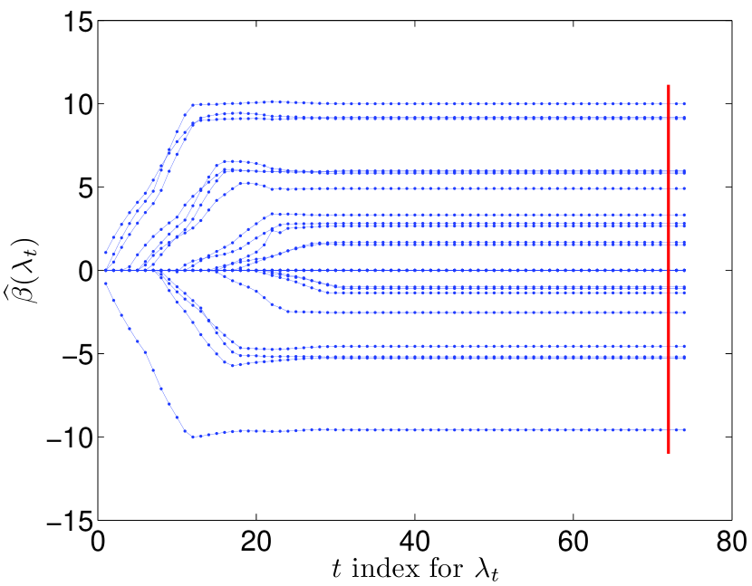
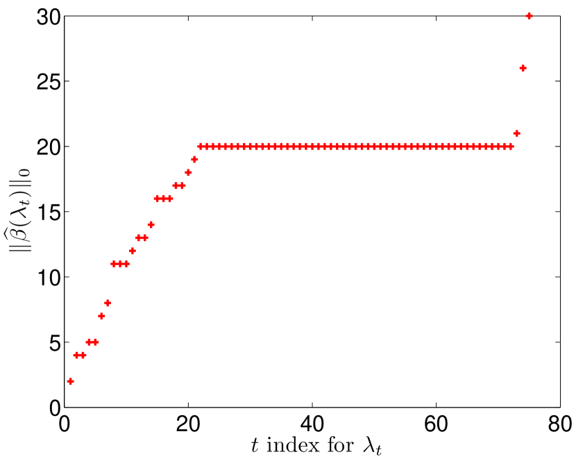
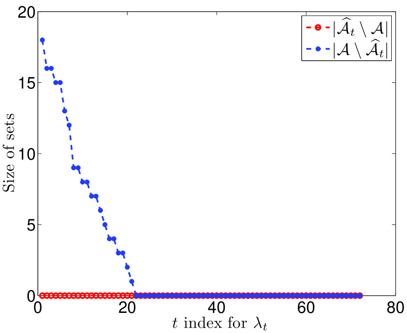
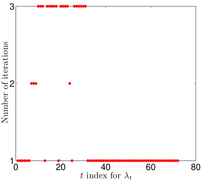
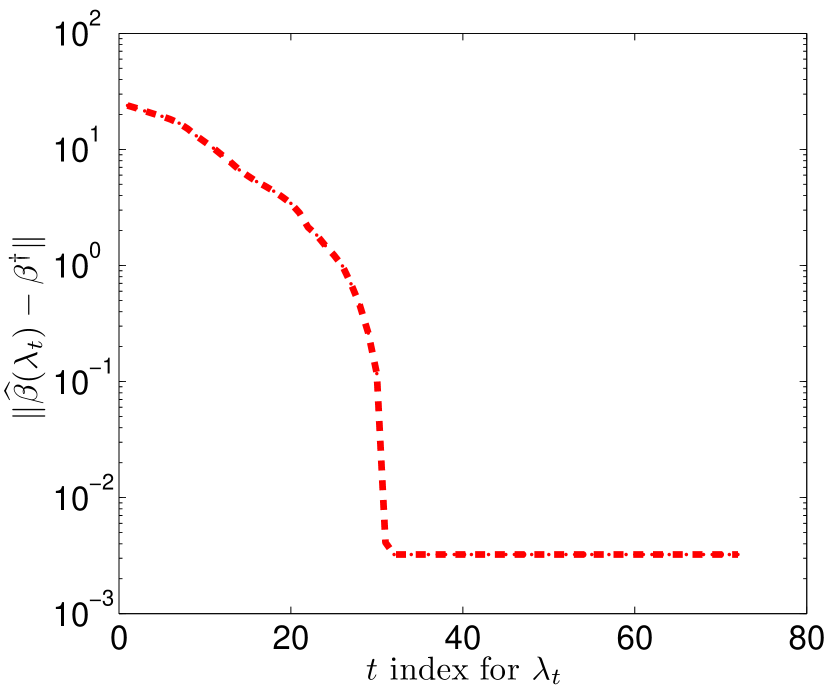
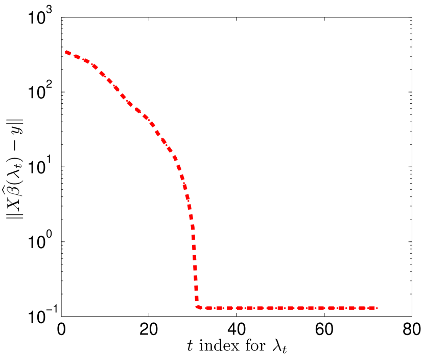
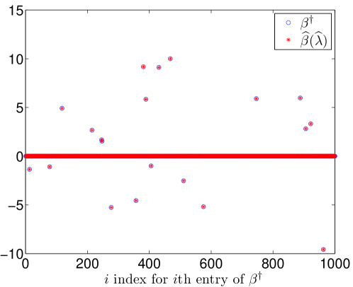
Fig. 1 shows the solution path of SSN and the size of the corresponding active set along the path. It also displays $\widehat{\lambda}$ and $\widehat{\beta}(\widehat{\lambda})$ (the red vertical line in the left panel) determined by the VC selector (46). To examine the local convergence property of the proposed algorithm, we present in Fig. 2 the change of the active sets and the number of iterations for each fixed $\lambda_{t}$ along the path $\lambda_{0}>\lambda_{1}>\cdots>\widehat{\lambda}$. We see that $\widehat{\mathcal{A}}_{t}\subset\mathcal{A}$, and the size $|\widehat{\mathcal{A}}_{t}|$ increases monotonically as the path proceeds and eventually equals the true model size $|\mathcal{A}|$. In particular, at each $\lambda_{t+1}$ with $\widehat{\beta}(\lambda_{t})$ as the initial value, SSN reaches convergence within one iteration in the latter part of the path. Fig. 3 displays the estimation error $\|\widehat{\beta}(\lambda_{t})-\beta^{\dagger}\|$ and the prediction error (i.e., the residual) $\|X\widehat{\beta}(\lambda_{t})-y\|$ along the path, as well as the underlying true $\beta^{\dagger}$ and the solution $\widehat{\beta}(\widehat{\lambda})$ selected by (46).

These numerical results strongly support the local superlinear convergence of the algorithm. They also demonstrate that the SSN algorithm yields estimates with good accuracy.

Figure 2: The change of the active sets (left panel) and the number of iterations (left panel) for each $\lambda_{t}$-problem along the warm-start path, where $\mathcal{A}$ is the true model and $\widehat{\mathcal{A}}_{t}\backslash\mathcal{A}$ ( $\mathcal{A}\backslash\widehat{\mathcal{A}}_{t}$) denotes the set difference of sets $\widehat{\mathcal{A}}_{t}$ and $\mathcal{A}$ ($\mathcal{A}$ and $\widehat{\mathcal{A}}_{t}$).

Figure 3: The estimation error $\|\widehat{\beta}(\lambda_{t})-\beta^{\dagger}\|$ (top left panel) and the prediction error $\|X\widehat{\beta}(\lambda_{t})-y\|$ (top right panel) along the path, and the underlying true $\beta^{\dagger}$ and the solution $\widehat{\beta}(\widehat{\lambda})$ selected by (46) (bottom panel).

IV-C Comparison with A CD-type Algorithm

We compare our SSN algorithm with a CD algorithm in [17] for solving (5), which is summarized in Algorithm 4. The stopping criterion at step 8 of Algorithm 4 is chosen to be either $k\geq J$ or $\|\beta^{k+1}-\beta^{k}\|\leq\delta$ with $\delta=1e-3$. We run CD on the same path as used in SSN with the same tuning parameter selection rule.

Algorithm 4 CD for MCP or SCAD

1:  Input: $X,y,\lambda,\gamma$, initial guess $\beta^{0}$ and $r^{0}=y-X\beta^{0}$. Set $k=0$.

2:  for $k=0,1,2,3,\ldots$ do

3:     for $i=1,2,\ldots,p$ do

4:        Calculate $z_{i}^{k}=X_{i}^{T}r^{k}+\beta_{i}^{k}$, where $X_{i}$ is the $i$th column of $X$ and $r^{k}=y-X\beta^{k}$ is the current residual value.

5:        Update $\beta^{k+1}_{i}\leftarrow T_{mcp}(z_{i}^{k};\lambda,\gamma)$ or $\beta^{k+1}_{i}\leftarrow T_{scad}(z_{i}^{k};\lambda,\gamma)$.

6:        Update $r^{k+1}\leftarrow r^{k}-(\beta^{k+1}_{i}-\beta^{k}_{i})X_{i}$.

7:     end for

8:     Check Stop conditionIf stopDenote the last iteration by $\widehat{\beta}$.Else$k:=k+1.$

9:  end for

10:  Output: $\widehat{\beta}$.

IV-C1 Efficiency and Accuracy

We set $p=1000$ and $2000$ with $n=\left\lfloor{p/5}\right\rfloor$ and $T=\left\lfloor{n/[2\log(p)]}\right\rfloor$, where $\left\lfloor{x}\right\rfloor$ denotes the integer part of $x$ for $x\geq 0$. We choose three levels of correlation $r=0.3,0.5$ and $0.7$, which correspond to weak, moderate and strong correlation. We consider two levels of noise: $\sigma=1$ (higher level) and $\sigma=0.1$ (lower level). The number of replications is $N=100$.

To further illustrate the efficiency and accuracy of SSN, we compare it with CD in terms of the average CPU time (Time, in seconds), the average estimated model size (MS) $N^{-1}\sum_{m=1}^{N}|\widehat{\mathcal{A}}^{(m)}|$, the proportion of correct models (CM, in percentage terms) $N^{-1}\sum_{m=1}^{N}I\{\widehat{\mathcal{A}}^{(m)}=\mathcal{A}\}$, the average $\ell_{\infty}$ absolute error (AE) $N^{-1}\sum_{m=1}^{N}\|\widehat{\beta}^{(m)}-\beta^{\dagger}\|_{\infty}$ and the average $\ell_{2}$ relative error (RE) $N^{-1}\sum_{m=1}^{N}(\|\widehat{\beta}^{(m)}-\beta^{\dagger}\|_{2}/\|\beta^{\dagger}\|_{2})$. The measures MS, CM, AE and RE evaluate the quality (accuracy) of the solutions. Clearly, the closer MS approaches to $T$, the closer CM approaches to $100\%$, and the smaller AE and RE, the higher the solution quality. The results are summarized in Table I.

TABLE I: Simulation results for CD and SSN with $n=\left\lfloor{p/5}\right\rfloor$ and $T=\left\lfloor{n/[2\log(p)]}\right\rfloor$ based on 100 independent runs. $(M,J)=(200,1)$.

p	r	$\sigma$	Penalty	Method	Time	MS	CM	AE	RE
1000	0.3	0.1	MCP	CD	1.3458	14.00	100%	0.0142	0.0014
				SSN	0.1920	14.00	100%	0.0183	0.0018
			SCAD	CD	1.7671	14.00	100%	0.0150	0.0015
				SSN	0.2068	14.00	100%	0.0188	0.0018
		1	MCP	CD	0.8790	14.00	100%	0.1493	0.0147
				SSN	0.1228	14.00	100%	0.1504	0.0148
			SCAD	CD	1.1659	13.90	99%	0.1778	0.0174
				SSN	0.1418	13.97	99%	0.1580	0.0152
	0.5	0.1	MCP	CD	1.3387	14.00	100%	0.0153	0.0015
				SSN	0.1849	13.78	98%	0.1489	0.0132
			SCAD	CD	1.7413	14.00	100%	0.0148	0.0015
				SSN	0.2238	14.00	100%	0.0187	0.0018
		1	MCP	CD	0.8668	13.92	98%	0.1730	0.0171
				SSN	0.1309	13.92	98%	0.1735	0.0171
			SCAD	CD	1.1434	13.82	97%	0.1809	0.0191
				SSN	0.1509	13.97	99%	0.1492	0.0147
	0.7	0.1	MCP	CD	1.3677	14.00	100%	0.0149	0.0015
				SSN	0.1773	13.20	90%	0.3823	0.0434
			SCAD	CD	1.7679	14.00	100%	0.0146	0.0015
				SSN	0.2168	14.00	100%	0.0190	0.0019
		1	MCP	CD	0.8786	13.95	98%	0.1787	0.0169
				SSN	0.1175	12.35	76%	0.9406	0.0983
			SCAD	CD	1.1441	13.47	91%	0.4013	0.0424
				SSN	0.1484	14.01	97%	0.1761	0.0166
2000	0.3	0.1	MCP	CD	3.0636	26.00	100%	0.0113	0.0011
				SSN	0.7697	26.00	100%	0.0164	0.0015
			SCAD	CD	3.8884	26.00	100%	0.0119	0.0011
				SSN	0.8128	26.00	100%	0.0169	0.0016
		1	MCP	CD	2.0280	26.00	100%	0.1165	0.0108
				SSN	0.5568	26.00	100%	0.1169	0.0108
			SCAD	CD	2.5903	26.00	100%	0.1176	0.0109
				SSN	0.5928	26.00	100%	0.1178	0.0109
	0.5	0.1	MCP	CD	3.0998	26.00	100%	0.0122	0.0010
				SSN	0.6672	26.00	100%	0.0177	0.0015
			SCAD	CD	3.9453	26.00	100%	0.0117	0.0011
				SSN	0.7062	26.00	100%	0.0168	0.0015
		1	MCP	CD	2.0312	26.00	100%	0.1204	0.0104
				SSN	0.4682	26.00	100%	0.1206	0.0105
			SCAD	CD	2.6170	26.00	100%	0.1181	0.0105
				SSN	0.5067	26.00	100%	0.1187	0.0105
	0.7	0.1	MCP	CD	3.1308	26.00	100%	0.0121	0.0011
				SSN	0.6379	24.09	84%	0.6352	0.0607
			SCAD	CD	3.9982	26.00	100%	0.0117	0.0011
				SSN	0.7078	26.00	100%	0.0178	0.0016
		1	MCP	CD	2.0787	26.00	100%	0.1189	0.0107
				SSN	0.5186	24.59	82%	0.5718	0.0561
			SCAD	CD	2.6466	25.93	97%	0.1547	0.0134
				SSN	0.5884	26.00	98%	0.1302	0.0115

For each $(p,r,\sigma)$ combination, we see from Table I that SSN is faster than CD for both MCP and SCAD. Specifically, SSN is about $3\sim 9$ times faster than CD. For a given penalty and algorithm, the CPU time decreases as $\sigma$ increases, increases linearly with $p$, and is fairly robust to the choice of $r$, with the other two parameters in the 3-tuple $(p,r,\sigma)$ fixed. For SCAD, SSN and CD are comparable in terms of solution quality. Unsurprisingly, larger $\sigma$ will degrade the accuracy for both CD and SSN. When the correlation level is low or moderate (i.e., $r=0.3$ or $0.5$), similar phenomena hold for MCP. For MCP with high correlation data (i.e., $r=0.7$), CD provides a more accurate solution than SSN does, which is due to the choice of $\gamma=2.7$ for MCP. In fact, simulations not reported in Table I show that if we increase the value of $\gamma$ for MCP, say $\gamma=4$, SSN can also produce similar solution quality comparing with CD. Please also refer to Remark 1 for relevant discussions. Overall, the simulation results in Table I show that SSN outperforms CD in terms of CPU time while producing solutions of comparable quality.

IV-C2 Influence of Model Parameters

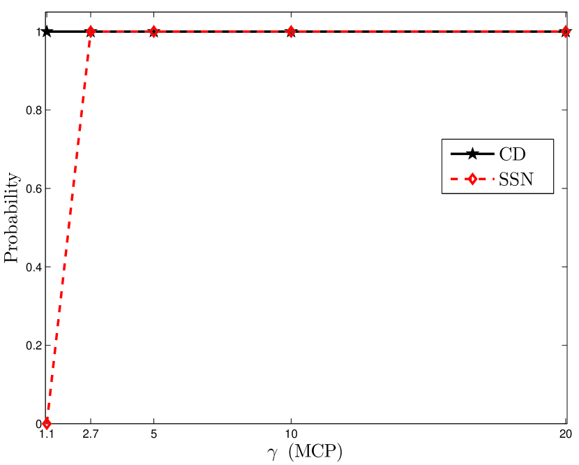
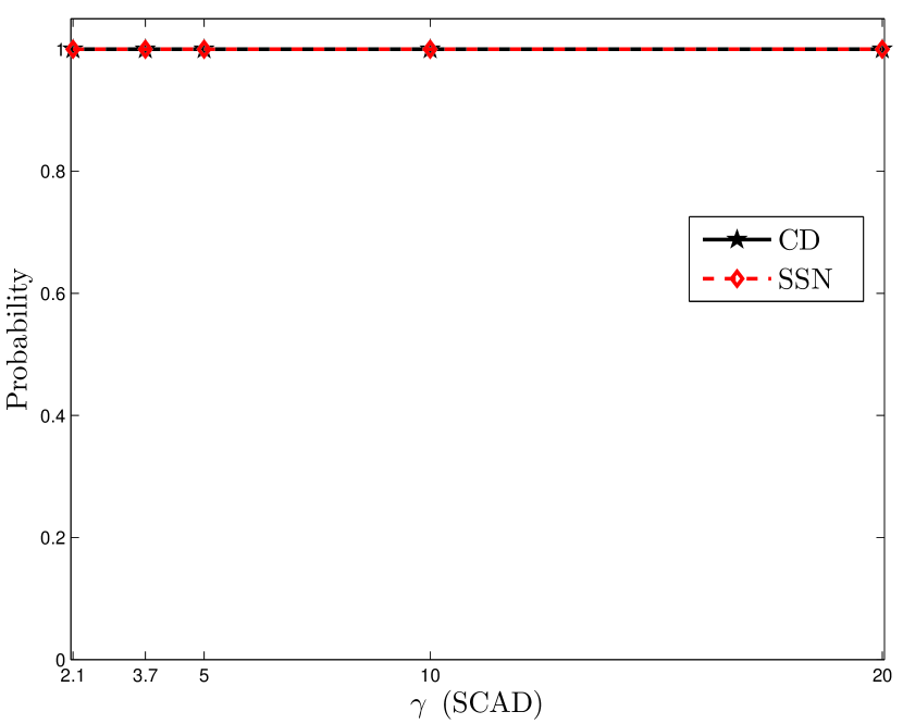
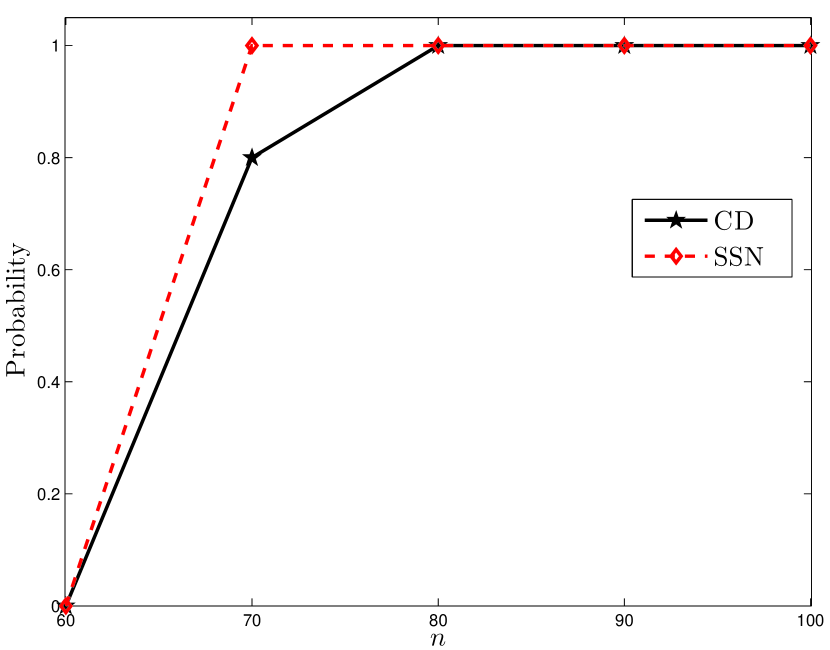
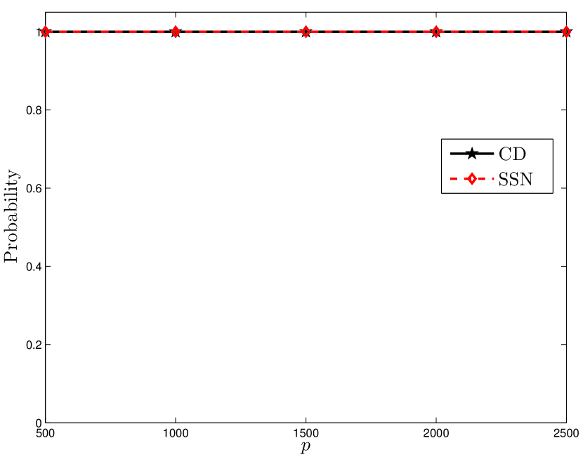
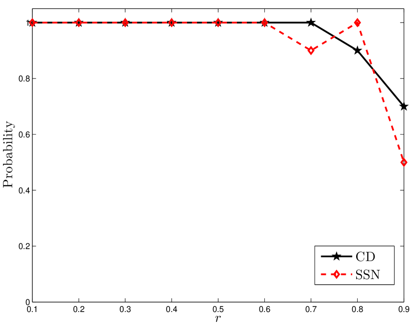
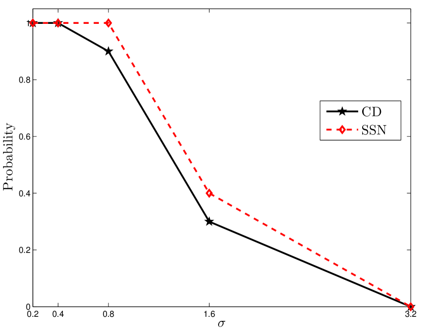
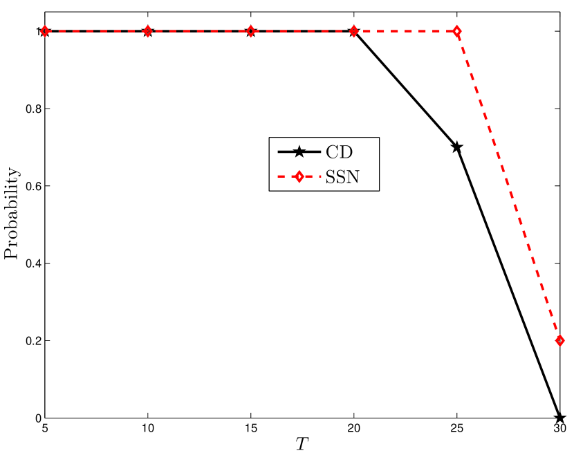
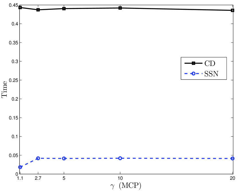
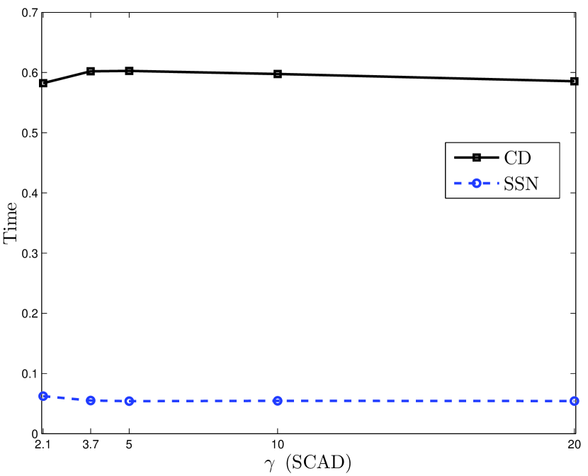
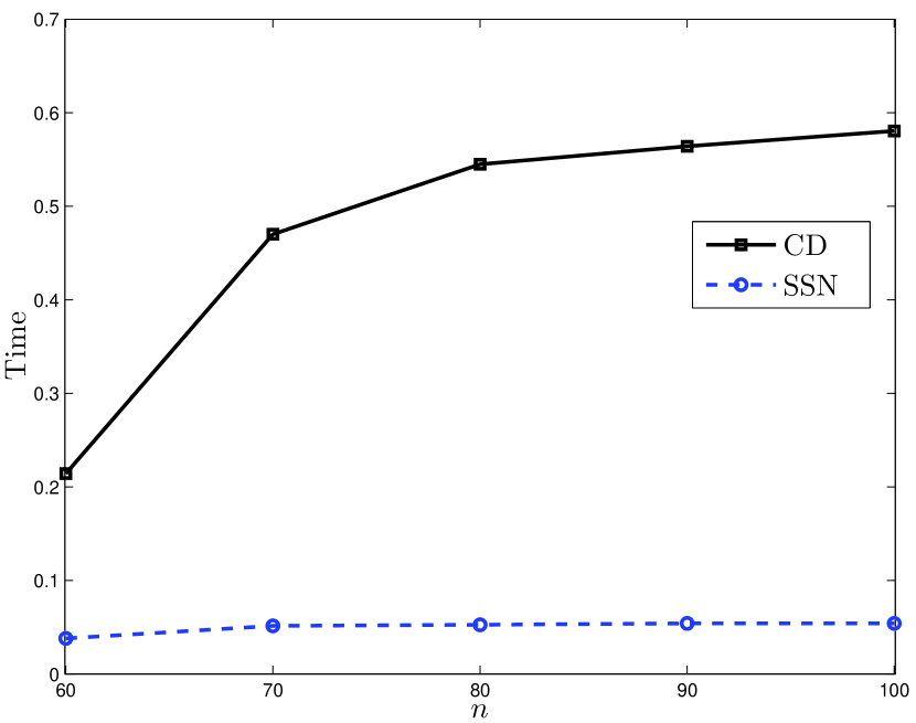
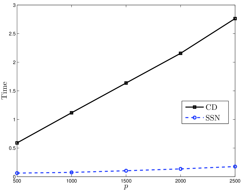
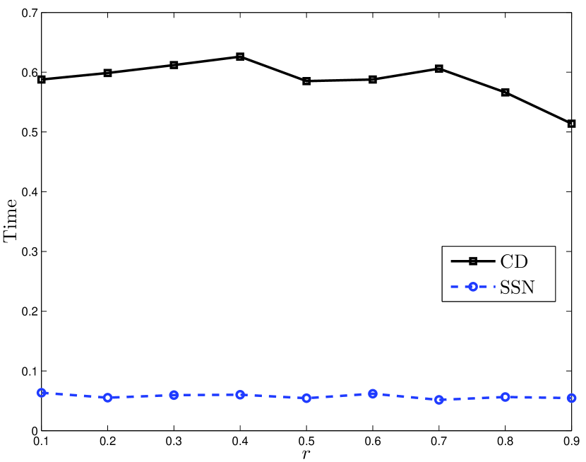
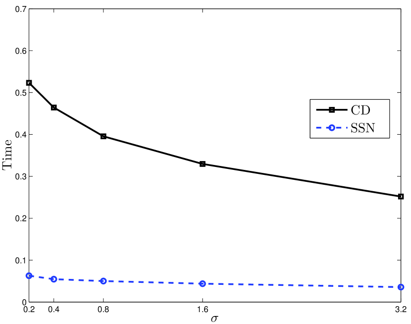
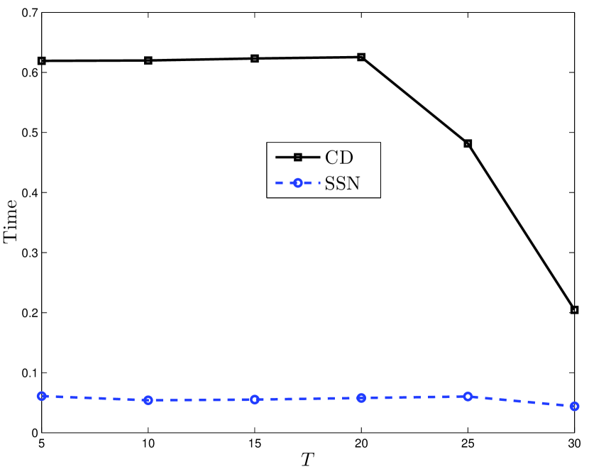
We now consider the effects of each of the model parameters $(\gamma,n,p,r,\sigma,T)$ on the performance of SSN and CD more closely in terms of the exact support recovery probability (Probability), i.e., the percentage of $\widehat{\mathcal{A}}$ agrees with $\mathcal{A}$, and the CPU time (Time, in seconds). For the sake of simplicity, we consider $\gamma$ for both MCP and SCAD, and only consider $(n,p,r,\sigma,T)$ for SCAD, since MCP has similar patterns with respect to the change in $(n,p,r,\sigma,T)$. Results of Probability and Time averaged over $10$ independent runs are given in Fig. 4 and Fig. 5, respectively. The parameters for the solvers are set as follows.

Influence of the concavity parameter $\gamma$

Data are generated from the model with $(\gamma\in\{1.1,2.7,5,10,20\},n=100,p=500,r=0.1,\sigma=0.1,T=10)$ for MCP and $(\gamma\in\{2.1,3.7,5,10,20\},n=100,p=500,r=0.1,\sigma=0.1,T=10)$ for SCAD.

Influence of the sample size $n$

Data are generated from the model with $(\gamma=3.7,n=60:10:100,p=500,r=0.1,\sigma=0.1,T=10)$.

Influence of the dimension $p$

Data are generated from the model with $(\gamma=3.7,n=100,p=500:500:2500,r=0.1,\sigma=0.1,T=10)$.

Influence of the correlation level $r$

Data are generated from the model with $(\gamma=3.7,n=100,p=500,r=0.1:0.1:0.9,\sigma=0.1,T=10)$.

Influence of the noise level $\sigma$

Data are generated from the model with $(\gamma=3.7,n=100,p=500,r=0.1,\sigma\in\{0.2,0.4,0.8,1.6,3.2\},T=10)$.

Influence of the sparsity level $T$

Data are generated from the model with $(\gamma=3.7,n=100,p=500,r=0.1,\sigma=0.1,T=5:5:30)$.

The results shown in Fig. 4 and Fig. 5 demonstrate that two solvers tend to give similar curve changing trends overall. However, SSN is considerably faster than CD with better (or comparable) accuracy, which is consistent with the simulation results in Table I. In particular, it’s good to see, as shown in Fig. 5, that the CPU time of SSN is insensitive to each of the model parameters $(\gamma,n,p,r,\sigma,T)$, which means SSN could be efficiently scaled up to other larger datasets.

Figure 4: Numerical results of the influence of the model parameters on the exact support recovery probability.

Figure 5: Numerical results of the influence of the model parameters on the CPU time.

IV-C3 Breast Cancer Data Example

Mining biological data are hot issues in machine learning fields [40, 41, 42, 43, 44]. SCAD and MCP are two popular supervised learning methods used to find sparse structures in high-dimensional data such as gene expression data [17, 45]. Here we analyze the breast cancer gene expression data from The Cancer Genome Atlas (TCGA) project to illustrate the application of SSN in high-dimensional settings. This data set, which is named bcTCGA, is available at http://myweb.uiowa.edu/pbreheny/data/bcTCGA.RData. It contains expression measurements of 17814 genes from 536 patients. There are $491$ genes with missing data, which we have excluded. We restrict our attention to the $17323$ genes without any missing values. The response variable $y$ represents the expression levels of gene BRCA1, which is the first gene identified that increases the risk of early onset breast cancer. The design matrix $X$ is a $536\times 17322$ matrix, which contains the remaining expression measurements of 17322 genes. Because BRCA1 is likely to interact with many other genes, it is of interest to find genes with expression levels related to that of BRCA1.

We fit a penalized linear regression model to find genes that are related to BRCA1. We analyze this data set using the proposed SSN algorithm. We also compare the results with those from the CD algorithm and the adaptive LASSO (ALASSO) [46]. The results from the ALASSO are computed using the ncvreg [17] and glmnet [47], which are R wrappers for C/Fortran. The following commands complete the main part of the ALASSO computation:

ptm <- proc.time()
library(ncvreg)
fit <- ncvreg(X, y, penalty=’lasso’)
beta0 <- coef(fit,which=which.min(BIC(fit)))[-1]
weight <- abs(beta0)^(-1)
weight <- pmin(weight,1e10)
library(glmnet); set.seed(0)
cvfit <- cv.glmnet(X,y,nfolds=10,penalty.factor=weight)
betahat <- coef(cvfit, s=’lambda.1se’)
ptm <- (proc.time()-ptm)[3]

We set $\gamma=4$ and $3.7$ for MCP and SCAD, respectively. Table II contains the selected genes the corresponding estimated coefficients, the CPU time (Time) and the prediction error (PE). As shown in this table, ALASSO, MCP-CD, MCP-SSN, SCAD-CD and SCAD-SSN identify 8, 5, 10, 13 and 8 genes, respectively. We observe that some genes, such as C17orf53, DTL, NBR2, SPAG5 and VPS25, are selected by at least three solvers, and in particular, all methods capture the gene NBR2 with relatively large absolute estimated coefficients. NBR2 is adjacent to BRCA1 on chromosome 17, and recent experimental evidence indicates that the two genes share a promoter [48]. It is also observed from Table II that SSN is faster than ALASSO and CD while producing smaller (or comparable) PE.

TABLE II: Analysis of the bcTCGA dataset. Estimated coefficients of different methods are provided. The zero entries correspond to variables omitted.

				MCP			SCAD
No.	Term	Gene	ALASSO	CD	SSN		CD	SSN
	Intercept		-0.6786	-0.7361	-0.4888		-0.9269	-0.4552
1	$\beta_{1743}$	C17orf53	0.1208	0	0.0240		0.0979	0.3883
2	$\beta_{2739}$	CCDC56	0	0	0		0.0484	0
3	$\beta_{2964}$	CDC25C	0	0	0		0.0360	0.0444
4	$\beta_{2987}$	CDC6	0	0	0		0.0089	0
5	$\beta_{3105}$	CENPK	0	0	0		0.0125	0
6	$\beta_{4543}$	DTL	0.2544	0.2883	0.2223		0.0886	0.0746
7	$\beta_{6224}$	GNL1	0	0	-0.1452		0	-0.1025
8	$\beta_{7709}$	KHDRBS1	0.1819	0	0		0	0
9	$\beta_{7719}$	KIAA0101	0	0	0		0	0.0675
10	$\beta_{8782}$	LSM12	0	0.0432	0		0	0
11	$\beta_{9230}$	MFGE8	0	0	-0.0273		0	-0.0972
12	$\beta_{9941}$	NBR2	0.4496	0.3984	0.5351		0.2408	0.5319
13	$\beta_{11091}$	PCGF1	0	0	-0.0968		0	0
14	$\beta_{12146}$	PSME3	0.1439	0	0		0.0746	0
15	$\beta_{13518}$	SETMAR	0	0	-0.0807		0	0
16	$\beta_{14296}$	SPAG5	0.0035	0.0598	0.2370		0.0117	0.0688
17	$\beta_{14397}$	SPRY2	0	0	0		-0.0058	0
18	$\beta_{15122}$	TIMELESS	0	0	0		0.0322	0
19	$\beta_{15535}$	TOP2A	0	0	0		0.0299	0
20	$\beta_{15882}$	TUBA1B	0.0857	0	0		0	0
21	$\beta_{16315}$	VPS25	0.2560	0.2372	0.3581		0.0998	0
22	$\beta_{16640}$	ZBTB26	0	0	-0.1015		0	0
	Time		14.7600	28.7712	3.3998		30.8354	3.1835
	PE		0.2116	0.2344	0.1837		0.2639	0.2117

To further evaluate the performance of SSN relative to CD on the quality of variable selection, we conduct the cross-validation procedure similar to [49, 50]. We conduct $50$ random partitions of the data. For each partition, we randomly choose $3/4$ observations and $1/4$ observations as the training and test data, respectively. We compute the CPU time (Time, in seconds) and the model size (MS, i.e., the number of selected genes) using the training data, and calculate the PE based on the test data. Table III presents the average values over $50$ random partitions, along with corresponding standard deviations in the parentheses. As shown in Table III, SSN performs better than CD in terms of the CPU time while producing comparable PE. Based on $50$ random partitions, we also report the selected genes and their corresponding frequency (Freq) of being selected in Table IV. We only list genes with frequency greater than or equal to 5 counts. For each scenario, the gene NBR2 is the top 1 gene ranked according to the frequency and has a significantly higher frequency than other genes, which is consistent with the findings of Table II and [48], and largely implies this gene is most closely related to BRCA1.

TABLE III: The CPU time (Time), model size (MS) and prediction error (PE) averaged across $50$ random partitions of the real data (numbers in parentheses are standard deviations)

Penalty	Method	Time	MS	PE
MCP	CD	25.3317(1.4440)	7.02(2.8820)	0.2761(0.0451)
	SSN	2.5452(0.4913)	9.46(3.7591)	0.2914(0.0568)
SCAD	CD	26.0625(1.4431)	9.46(3.3025)	0.3190(0.0624)
	SSN	2.5736(0.4382)	9.00(4.4584)	0.2647(0.0471)

TABLE IV: Frequency table for $50$ random partitions of the real data. To save space, only the genes with Freq $\geq 5$ are listed.

MCP						SCAD
CD			SSN			CD			SSN
Gene	Freq		Gene	Freq		Gene	Freq		Gene	Freq
NBR2	50		NBR2	46		NBR2	49		NBR2	50
DTL	36		C17orf53	40		DTL	47		C17orf53	34
VPS25	31		MFGE8	11		VPS25	47		DTL	17
C17orf53	25		VPS25	10		C17orf53	47		VPS25	13
CCDC56	12		GNL1	10		PSME3	38		MFGE8	11
CDC25C	12		PSME3	8		TOP2A	34		KLHL13	10
SPAG5	12		C3orf10	8		CCDC56	26		C10orf76	8
PSME3	12		DTL	7		TIMELESS	26		GNL1	8
LSM12	11		CMTM5	7		CDC25C	20		ZBTB26	8
TOP2A	8		FAM103A1	7		CENPK	15		TIMELESS	7
KLHL13	8		KIAA0101	7		SPAG5	14		DYNLL1	6
SPRY2	8		ZYX	6		CCDC43	12		FAM103A1	6
NPR2	7		MCM6	6		CDC6	12		KHDRBS1	6
TUBA1B	7		SETMAR	6		SPRY2	9		SETMAR	6
TIMELESS	6		FBXO18	6		RDM1	8		TOP2A	6
KIAA0101	6		SPAG5	6		CENPQ	6		CMTM5	6
CENPK	5		LMNB1	6		TUBG1	6		FGFRL1	6
CRBN	5		KHDRBS1	6					PSME3	5
VDAC1	5		ATAD1	6					LMNB1	5
CMTM5	5		KLHL13	6					ZNF189	5
CDC6	5		AASDH	5					CENPQ	5
			YTHDC2	5					HMGN2	5
			DYNLL1	5					CRBN	5
			TUBG1	5
			HMGN2	5
			CENPQ	5
			C10orf30	5

IV-D Comparison with the DCPN

We conduct numerical experiments to compare DCPN and SSN. The implementation setting and comparison metrics are given in Sections IV-A and IV-C, respectively. The noise level $\sigma=1$ is fixed. The DCPN is implemented using the picasso package [37, 51]. For both solvers, we use the HBIC selector to choose the tuning parameters. We set $\gamma=4$ and $3.7$ for MCP and SCAD, respectively. Simulation results are summarized in Table V.

TABLE V: Simulation results for DCPN and SSN with $n=\left\lfloor{p/5}\right\rfloor$ and $T=\left\lfloor{n/[2\log(p)]}\right\rfloor$ based on 10 independent runs. $(M,J)=(100,1)$ and $\sigma=1$.

$p$	$r$	Penalty	Method	Time	MS	CM	AE	RE
1000	0.3	MCP	DCPN	0.147	14.0	100%	0.9821	0.0620
			SSN	0.057	14.0	100%	0.1456	0.0142
		SCAD	DCPN	0.145	14.0	100%	0.9870	0.0654
			SSN	0.059	14.0	100%	0.1456	0.0142
	0.7	MCP	DCPN	0.144	15.0	0%	0.4258	0.0355
			SSN	0.045	11.9	80%	1.3921	0.1255
		SCAD	DCPN	0.154	15.0	0%	0.5866	0.0467
			SSN	0.059	14.0	100%	0.1693	0.0149
2000	0.3	MCP	DCPN	0.286	26.0	100%	1.0080	0.0623
			SSN	0.209	26.0	100%	0.1210	0.0104
		SCAD	DCPN	0.248	26.0	100%	1.0436	0.0715
			SSN	0.222	26.0	100%	0.1210	0.0104
	0.7	MCP	DCPN	0.282	26.9	10%	0.4845	0.0424
			SSN	0.200	23.5	90%	0.9125	0.0998
		SCAD	DCPN	0.262	26.9	10%	0.6178	0.0546
			SSN	0.222	26.0	100%	0.1172	0.0108

For each combination, we observed from Table V that SSN is faster than DCPN, see the column that includes the values of Time. Here we should note that SSN is implemented in Matlab, while DCPN uses the picasso package which is a R wrapped C solver. So strictly speaking, this is not a fair comparison, but is actually in favor of DCPN. In addition, the CPU time generally increases linearly with $p$, and is relatively robust to the choice of $r$. When the correlation is low (i.e., $r=0.3$), both solvers can select the true model 100 percent correctly, while SSN can produce solutions with smaller AE and RE comparing with DCPN. At high correlation level (i.e., $r=0.7$), the SSN still behaves well in terms of CM, while the DCPN almost fails on this metric, and both solvers share comparable AE and RE. In summary, the comparison results in Table V show good performance of SSN in terms of both efficiency and accuracy.

V Conclusion

Starting from the KKT conditions we developed a SSN algorithm for the MCP and SCAD regularized learning problems in high-dimensional settings. We established the local superlinear convergence of SSN and analyzed its computational complexity. Combining with the VC or HBIC tuning parameter selector with warm start, we obtain the solution path and select the tuning parameters in a fast and stable way. Numerical comparisons with CD and DCPN demonstrate the efficiency and accuracy of SSN. A Matlab package ssn-nonconvex that implements the proposed algorithms is available at http://faculty.zuel.edu.cn/tjyjxxy/jyl/list.htm.

There are several avenues for further research. First, SSN can be extended to structured sparsity learning problems such as group MCP/SCAD [52, 30], or to other learning problems with general nonlinear loss functions [53, 54], especially for those related to deep neural networks (DNNs) [55, 56, 57]. Second, the authors in [36] prove nice statistical convergence results of their Newton type algorithm in high dimensions. Inspired by [36], bounding the statistical errors of our SSN algorithm along the solution path may be one possible direction to further understanding of the SSN. Third, semi-smooth Newton methods converges to KKT points supperlinearly but locally, we adopt simple continuation strategy to globalize it. Globalization via smoothing Newton methods [58, 59, 60] is also of immense interest in future work.

Unless otherwise stated, we only give the proofs for MCP since the counterparts for SCAD are similar.

-A Proof of Lemma 1

Proof:

See [17] and [18]. ∎

-B Proof of Theorem 1

Proof:

Let $\widehat{\beta}\in\mathbb{R}^{p}$ be a global minimizer of

$$E_{mcp}(\beta):=\frac{1}{2}\|X\beta-y\|^{2}_{2}+\sum_{i=1}^{p}P_{mcp}(\beta_{i};\lambda,\gamma).$$

Define

$$f_{i}(t)=E_{mcp}(\widehat{\beta}_{1},...,\widehat{\beta}_{i-1},t,\widehat{\beta}_{i+1,},...,\widehat{\beta}_{p}),i=1,2,...,p.$$

Then, by definition $\widehat{\beta}_{i}$ is a global minimizer of the scalar function $f_{i}(t)$. Some algebra shows that the minimizer of $f_{i}(t)$ is also the minimizer of $\frac{1}{2}(t-(\widehat{\beta}_{i}+X_{i}^{T}(y-X\widehat{\beta})))^{2}+P_{mcp}(t;\lambda,\gamma)$. Then $\widehat{\beta}_{i}=T_{mcp}(\widehat{\beta}_{i}+X_{i}^{T}(y-X\widehat{\beta});\lambda,\gamma)$ by Lemma 1. (15) - (16) follow from the definitions of $G=X^{T}X,$ $\widetilde{y}=X^{T}y$ and $\mathbb{T}(\cdot;\lambda,\gamma)$.

Conversely, assume that $(\widehat{\beta},\widehat{d})$ satisfies (15) - (16). Then $\forall i,\widehat{\beta}_{i}=T_{mcp}(\widehat{\beta}_{i}+X_{i}^{T}(y-X\widehat{\beta});\lambda,\gamma)$, which implies that $\widehat{\beta}_{i}$ is a minimizer of the $f_{i}(t)$ defined above. This shows $\widehat{\beta}$ is a coordinate-wise minimizer of $E_{mcp}$. By Lemma 3.1 in [61], $\widehat{\beta}$ is also a stationary point. ∎

-C Proof of Lemma 2

Proof:

Observing that both $T_{scad}(\cdot;\lambda,\gamma)$ and $T_{mcp}(\cdot;\lambda,\gamma)$ are piecewise linear functions on $\mathbb{R}^{1}$, it suffices to prove that the piecewise linear scalar function

$$f(t)=\left\{\begin{aligned} &k_{1}t+b_{1},\quad if\quad t\leq t_{0},\\ &k_{2}t+b_{2},\quad if\quad t>t_{0}.\end{aligned}\right.$$

is Newton differentiable with

$$\nabla_{N}f(t)=\left\{\begin{array}[]{ll}$\text{$k_{1}$}$,&\text{$t<t_{0},$}\\ $\text{$r$ }$\in\mathbb{R}^{1},&\text{$t=t_{0},$}\\ $\text{$k_{2}$}$,&\text{$t_{0}<t.$}\\ \end{array}\right.$$ (49)

where $k_{1},k_{2},b_{1},b_{2},t_{0}$ are any constants satisfying $k_{1}t_{0}+b_{1}=k_{2}t_{0}+b_{2}$. Indeed, let

$$D(t+h)h=\left\{\begin{array}[]{ll}$\text{$k_{1}h$}$,&\text{$t<t_{0},$}\\ $\text{$k_{2}h$}$,&\text{$t_{0}<t,$}\\ \end{array}\right.$$

and $G(t_{0})h=rh$ with an arbitrary $r\in\mathbb{R}$, then $|f(t+h)-f(t)-D(t+h)h|/|h|\longrightarrow 0$ as $|h|\longrightarrow 0.$ ∎

-D Proof of Theorem 2

Proof:

Let

$$b(t;\lambda,\gamma)=\left\{\begin{array}[]{ll}$ 0$,&\text{$|t|\leq\lambda,$}\\ $ 1/(1-1/$\gamma$)$,&\text{$\lambda<|t|<\gamma\lambda,$}\\ $ 1$,&\text{$\gamma\lambda\geq|t|,$}\\ \end{array}\right.$$

$\textbf{b}(x;\lambda,\gamma)=\textrm{diag}(b(x_{1};\lambda,\gamma),...,b(x_{p};\lambda,\gamma))$, $g_{i}(x)=T_{mcp}(e_{i}^{T}x;\lambda,\gamma):x\in\mathbb{R}^{p}\rightarrow\mathbb{R}^{1},i=1,\ldots,p$, and $\mathbb{T}(x;\lambda,\gamma)=(g_{1}(x),...,g_{p}(x))^{T}$, where the column vector $e_{i}$ is the $i_{th}$ orthonormal basis in $\mathbb{R}^{p}$.

It follows from Lemma 2 and (9)-(11) that $b(t;\lambda,\gamma)\in\nabla_{N}{T}_{mcp}(t)$ and

$$\textbf{b}(x;\lambda,\gamma)\in\nabla_{N}\mathbb{T}(x;\lambda,\gamma).$$ (50)

Then, by (50) and (9)-(11) the vector value function $F_{1}(\beta;d)$ is Newton differentiable and

$$\begin{bmatrix}H_{11}^{k}&H_{12}^{k}\\ \end{bmatrix}\in\nabla_{N}F_{1}(z^{k}_{mcp}),$$ (51)

where $H_{11}^{k}$ and $H_{12}^{k}$ are given in (25). By (9)-(11), $F_{2}(\beta;d)$ is Newton differentiable and

$$\begin{bmatrix}H_{21}^{k}&H_{22}^{k}\\ \end{bmatrix}\in\nabla_{N}F_{2}(z^{k}_{mcp}),$$ (52)

where $H_{21}^{k}$ and $H_{22}^{k}$ are also given in (25). It follows from (51)-(52) and (9)-(11) that $H_{mcp}^{k}\in\nabla_{N}F_{mcp}(z^{k}_{mcp})$.

The uniform boundedness of $(H_{mcp}^{k})^{-1}$ is derived similarly as the proof of Theorem 2.6 in [50]. ∎

-E Proof of Theorem 3

Proof:

Let $z^{k}_{mcp}$ be sufficiently close to $z^{*}_{mcp}$, which is a root of $F_{mcp}$. By the definition of the Newton derivative, we have

$$\|H^{k}_{mcp}(z^{k}_{mcp}-z^{*}_{mcp})-F_{mcp}(z^{k}_{mcp})+F_{mcp}(z^{*}_{mcp})\|_{2}$$ (53)

$$\leq\epsilon\|z^{k}_{mcp}-z^{*}_{mcp}\|_{2},$$

where $\epsilon\rightarrow 0$ as $z^{k}_{mcp}\rightarrow z^{*}_{mcp}$. Then, by the definition of SSN and the fact that $F_{mcp}(z^{*}_{mcp})=0$, we get

$$\|z^{k+1}_{mcp}-z^{*}_{mcp}\|_{2}$$

$$=\|z^{k}_{mcp}-(H^{k}_{mcp})^{-1}F_{mcp}(z^{k}_{mcp})-z^{*}_{mcp}\|_{2}$$

$$=\|z^{k}_{mcp}-(H^{k}_{mcp})^{-1}F_{mcp}(z^{k}_{mcp})-z^{*}_{mcp}+(H^{k}_{mcp})^{-1}F_{mcp}(z^{*}_{mcp})\|_{2}$$

$$\leq\|(H^{k}_{mcp})^{-1}\|\|H^{k}_{mcp}(z^{k}_{mcp}-z^{*}_{mcp})-F_{mcp}(z^{k}_{mcp})+F_{mcp}(z^{*}_{mcp})\|_{2}.$$

$$\leq M_{\gamma}\epsilon\|z^{k}_{mcp}-z^{*}_{mcp}\|_{2}.$$

The last inequality follows from (53) and the uniform boundedness of $(H^{k}_{mcp})^{-1}$ proved in Theorem 2. Therefore, the sequence $z_{mcp}^{k}$ generated by Algorithm 2 converges to $z_{mcp}^{*}$ locally and superlinearly. ∎

References

- [1] B. K. Natarajan, “Sparse approximate solutions to linear systems,” SIAM Journal on Computing, vol. 24, no. 2, pp. 227–234, 1995.
- [2] R. Tibshirani, “Regression shrinkage and selection via the lasso,” Journal of the Royal Statistical Society. Series B (Methodological), vol. 58, no. 1, pp. 267–288, 1996.
- [3] S. S. Chen, D. L. Donoho, and M. A. Saunders, “Atomic decomposition by basis pursuit,” SIAM Review, vol. 43, no. 1, pp. 129–159, 2001.
- [4] M. R. Osborne, B. Presnell, and B. A. Turlach, “A new approach to variable selection in least squares problems,” IMA Journal of Numerical Analysis, vol. 20, no. 3, pp. 389–403, 2000.
- [5] B. Efron, T. Hastie, I. Johnstone, and R. Tibshirani, “Least angle regression,” The Annals of Statistics, vol. 32, no. 2, pp. 407–499, 2004.
- [6] W. J. Fu, “Penalized regressions: the bridge versus the lasso,” Journal of Computational and Graphical Statistics, vol. 7, no. 3, pp. 397–416, 1998.
- [7] J. Friedman, T. Hastie, H. Höfling, and R. Tibshirani, “Pathwise coordinate optimization,” The Annals of Applied Statistics, vol. 1, no. 2, pp. 302–332, 2007.
- [8] T. T. Wu and K. Lange, “Coordinate descent algorithms for lasso penalized regression,” The Annals of Applied Statistics, vol. 2, no. 1, pp. 224–244, 2008.
- [9] E. J. Candes and T. Tao, “Decoding by linear programming,” IEEE Transactions on Information Theory, vol. 51, no. 12, pp. 4203–4215, 2005.
- [10] N. Meinshausen and P. Bühlmann, “High-dimensional graphs and variable selection with the lasso,” The Annals of Statistics, vol. 34, no. 3, pp. 1436–1462, 2006.
- [11] P. Zhao and B. Yu, “On model selection consistency of lasso,” Journal of Machine Learning Research, vol. 7, no. Nov, pp. 2541–2563, 2006.
- [12] J. Fan and R. Li, “Variable selection via nonconcave penalized likelihood and its oracle properties,” Journal of the American Statistical Association, vol. 96, no. 456, pp. 1348–1360, 2001.
- [13] C.-H. Zhang, “Nearly unbiased variable selection under minimax concave penalty,” The Annals of Statistics, vol. 38, no. 2, pp. 894–942, 2010.
- [14] K. Lange, D. R. Hunter, and I. Yang, “Optimization transfer using surrogate objective functions (with discussion),” Journal of Computational and Graphical Statistics, vol. 9, no. 1, pp. 1–59, 2000.
- [15] T. Zhang, “Analysis of multi-stage convex relaxation for sparse regularization,” Journal of Machine Learning Research, vol. 11, no. Mar, pp. 1081–1107, 2010.
- [16] H. Zou and R. Li, “One-step sparse estimates in nonconcave penalized likelihood models,” The Annals of Statistics, vol. 36, no. 4, pp. 1509–1533, 2008.
- [17] P. Breheny and J. Huang, “Coordinate descent algorithms for nonconvex penalized regression, with applications to biological feature selection,” The Annals of Applied Statistics, vol. 5, no. 1, p. 232, 2011.
- [18] R. Mazumder, J. H. Friedman, and T. Hastie, “Sparsenet: Coordinate descent with nonconvex penalties,” Journal of the American Statistical Association, vol. 106, no. 495, pp. 1125–1138, 2011.
- [19] G. Li and T. K. Pong, “Calculus of the exponent of Kurdyka–Łojasiewicz inequality and its applications to linear convergence of first-order methods,” Foundations of Computational Mathematics, vol. 18, no. 5, pp. 1199–1232, 2018.
- [20] B. Kummer, “Newton’s method for non-differentiable functions,” Advances in mathematical optimization, vol. 45, pp. 114–125, 1988.
- [21] L. Qi and J. Sun, “A nonsmooth version of newton’s method,” Mathematical programming, vol. 58, no. 1-3, pp. 353–367, 1993.
- [22] K. Ito and K. Kunisch, Lagrange multiplier approach to variational problems and applications. SIAM, 2008.
- [23] X. Chen, Z. Nashed, and L. Qi, “Smoothing methods and semismooth methods for nondifferentiable operator equations,” SIAM Journal on Numerical Analysis, vol. 38, no. 4, pp. 1200–1216, 2000.
- [24] D. L. Donoho and I. M. Johnstone, “Adapting to unknown smoothness via wavelet shrinkage,” Journal of the American Statistical Association, vol. 90, no. 432, pp. 1200–1224, 1995.
- [25] C.-H. Zhang and J. Huang, “The sparsity and bias of the lasso selection in high-dimensional linear regression,” The Annals of Statistics, vol. 36, no. 4, pp. 1567–1594, 2008.
- [26] Y. She, “Thresholding-based iterative selection procedures for model selection and shrinkage,” Electronic Journal of Statistics, vol. 3, pp. 384–415, 2009.
- [27] A. Beck and M. Teboulle, “A fast iterative shrinkage-thresholding algorithm for linear inverse problems,” SIAM Journal on Imaging Sciences, vol. 2, no. 1, pp. 183–202, 2009.
- [28] Y. Jiao, B. Jin, and X. Lu, “A primal dual active set with continuation algorithm for the -regularized optimization problem,” Applied and Computational Harmonic Analysis, vol. 39, no. 3, pp. 400–426, 2015.
- [29] Q. Fan, Y. Jiao, and X. Lu, “A primal dual active set algorithm with continuation for compressed sensing,” IEEE Transactions Signal Processing, vol. 62, no. 23, pp. 6276–6285, 2014.
- [30] Y. Jiao, B. Jin, and X. Lu, “Group sparse recovery via the penalty: theory and algorithm,” IEEE Transactions on Signal Processing, vol. 65, no. 4, pp. 998–1012, 2017.
- [31] Y. Shi, Y. Wu, D. Xu, and Y. Jiao, “An ADMM with continuation algorithm for non-convex SICA-penalized regression in high dimensions,” Journal of Statistical Computation and Simulation, vol. 88, no. 9, pp. 1826–1846, 2018.
- [32] J. Huang, Y. Jiao, X. Lu, and L. Zhu, “Robust decoding from 1-bit compressive sampling with ordinary and regularized least squares,” SIAM Journal on Scientific Computing, vol. 40, no. 4, pp. A2062–A2086, 2018.
- [33] L. Wang, Y. Kim, and R. Li, “Calibrating nonconvex penalized regression in ultra-high dimension,” The Annals of Statistics, vol. 41, no. 5, pp. 2505–2536, 2013.
- [34] Y. Shi, Y. Jiao, Y. Cao, and Y. Liu, “An alternating direction method of multipliers for mcp-penalized regression with high-dimensional data,” Acta Mathematica Sinica, English Series, vol. 34(12), pp. 1892–1906, 2018.
- [35] J. Huang, Y. Jiao, B. Jin, J. Liu, X. Lu, and C. Yang, “A unified primal dual active set algorithm for nonconvex sparse recovery,” arXiv preprint arXiv:1310.1147v4, 2018.
- [36] X. Li, L. Yang, J. Ge, J. Haupt, T. Zhang, and T. Zhao, “On quadratic convergence of DC proximal Newton algorithm in nonconvex sparse learning,” in Advances in Neural Information Processing Systems, 2017, pp. 2742–2752.
- [37] T. Zhao, H. Liu, T. Zhang et al., “Pathwise coordinate optimization for sparse learning: Algorithm and theory,” The Annals of Statistics, vol. 46, no. 1, pp. 180–218, 2018.
- [38] A. F. Izmailov and M. V. Solodov, Newton-type methods for optimization and variational problems. Springer, 2014.
- [39] S. Becker, J. Bobin, and E. J. Candès, “Nesta: A fast and accurate first-order method for sparse recovery,” SIAM Journal on Imaging Sciences, vol. 4, no. 1, pp. 1–39, 2011.
- [40] T. Hastie, R. Tibshirani, and J. Friedman, The elements of statistical learning: data mining, inference and prediction, 2nd ed. New York: Springer, 2009.
- [41] B. Gu and V. S. Sheng, “A solution path algorithm for general parametric quadratic programming problem,” IEEE Transactions on Neural Networks and Learning Systems, vol. 29, no. 9, pp. 4462–4472, 2017.
- [42] M. Mahmud, M. S. Kaiser, A. Hussain, and S. Vassanelli, “Applications of deep learning and reinforcement learning to biological data,” IEEE Transactions on Neural Networks and Learning Systems, vol. 29, no. 6, pp. 2063–2079, 2018.
- [43] J. Cai and X. Huang, “Modified sparse linear-discriminant analysis via nonconvex penalties,” IEEE Transactions on Neural Networks and Learning Systems, vol. 29, no. 10, pp. 4957–4966, 2018.
- [44] X. Li, H. Zhang, R. Zhang, Y. Liu, and F. Nie, “Generalized uncorrelated regression with adaptive graph for unsupervised feature selection,” IEEE Transactions on Neural Networks and Learning Systems, vol. 30, no. 5, pp. 1587–1595, 2019.
- [45] P. Breheny and J. Huang, “Group descent algorithms for nonconvex penalized linear and logistic regression models with grouped predictors,” Statistics and Computing, vol. 25, no. 2, pp. 173–187, 2015.
- [46] H. Zou, “The adaptive lasso and its oracle properties,” Journal of the American Statistical Association, vol. 101, no. 476, pp. 1418–1429, 2006.
- [47] J. Friedman, T. Hastie, and R. Tibshirani, “Regularization paths for generalized linear models via coordinate descent,” Journal of Statistical Software, vol. 33, no. 1, pp. 1–22, 2010.
- [48] P. J. Breheny, “Marginal false discovery rates for penalized regression models,” Biostatistics, vol. 20, no. 2, pp. 299–314, 2019.
- [49] J. Huang, S. Ma, and C.-H. Zhang, “Adaptive lasso for sparse high-dimensional regression models,” Statistica Sinica, vol. 18, pp. 1603–1618, 2008.
- [50] C. Yi and J. Huang, “Semismooth newton coordinate descent algorithm for elastic-net penalized huber loss regression and quantile regression,” Journal of Computational and Graphical Statistics, vol. 26, no. 3, pp. 547–557, 2017.
- [51] J. Ge, X. Li, H. Jiang, H. Liu, T. Zhang, M. Wang, and T. Zhao, Picasso: A sparse learning library for high dimensional data analysis in R and Python, 2017, version 1.2.0. [Online]. Available: https://CRAN.R-project.org/package=picasso
- [52] P. Breheny and J. Huang, “Group descent algorithms for nonconvex penalized linear and logistic regression models with grouped predictors,” Statistics and Computing, vol. 25, no. 2, pp. 173–187, 2015.
- [53] L. Liu, J. Liu, and D. Tao, “Dualityfree methods for stochastic composition optimization,” IEEE Transactions on Neural Networks and Learning Systems, vol. 30, no. 4, pp. 1205–1217, 2019.
- [54] D. Chang, S. Sun, and C. Zhang, “An accelerated linearly convergent stochastic L-BFGS algorithm,” IEEE Transactions on Neural Networks and Learning Systems, 2019. [Online]. Available: https://doi.org/10.1109/TNNLS.2019.2891088
- [55] S. Scardapane, D. Comminiello, A. Hussain, and A. Uncini, “Group sparse regularization for deep neural networks,” Neurocomputing, vol. 241, pp. 81–89, 2017.
- [56] C. Louizos, M. Welling, and D. P. Kingma, “Learning sparse neural networks through regularization,” in International Conference on Learning Representations, 2018. [Online]. Available: https://openreview.net/forum?id=H1Y8hhg0b
- [57] R. Ma, J. Miao, L. Niu, and P. Zhang, “Transformed regularization for learning sparse deep neural networks,” 2019. [Online]. Available: https://arxiv.org/abs/1901.01021
- [58] X. Chen, L. Qi, and D. Sun, “Global and superlinear convergence of the smoothing newton method and its application to general box constrained variational inequalities,” Mathematics of Computation of the American Mathematical Society, vol. 67, no. 222, pp. 519–540, 1998.
- [59] L. Qi and D. Sun, “A survey of some nonsmooth equations and smoothing newton methods,” in Progress in optimization. Springer, 1999, pp. 121–146.
- [60] L. Qi, D. Sun, and G. Zhou, “A new look at smoothing newton methods for nonlinear complementarity problems and box constrained variational inequalities,” Mathematical programming, vol. 87, no. 1, pp. 1–35, 2000.
- [61] P. Tseng, “Convergence of a block coordinate descent method for nondifferentiable minimization,” Journal of Optimization Theory and Applications, vol. 109, no. 3, pp. 475–494, 2001.