Integrating a Computational Perspective in Physics Courses

Abstract

In this contribution we discuss how to develop a physics curriculum for undergraduate students that includes computing as a central element. Our contribution starts with a definition of computing and pertinent learning outcomes and assessment studies and programs. We end with a discussion on how to implement computing in various physics courses by presenting our experiences from Michigan State University in the USA and the University of Oslo in Norway.

0.1 Introduction

Many important recent advances in our understanding of the physical world have been driven by large-scale computational modeling and data analysis, for example, the 2012 discovery of the Higgs boson, the 2013 Nobel Prize in chemistry for computational modeling of molecules, and the 2016 discovery of gravitational waves. Given the ubiquitous use in science and its critical importance to the future of science and engineering, scientific computing plays a central role in scientific investigations and is critical to innovation in most domains of our lives. It underpins the majority of today’s technological, economic and societal feats. We have entered an era in which huge amounts of data offer enormous opportunities. By 2020, it is also expected that one out of every two jobs in the STEM (Science, Technology, Engineering and Mathematics) fields will be in computing (Association for Computing Machinery, 2013, ACM2013 ).

These developments, needs and future challenges, as well as the developments that are now taking place within quantum computing, quantum information theory and data driven discoveries (data analysis and machine learning) will play an essential role in shaping future technological developments. Most of these developments require true cross-disciplinary approaches and bridge a vast range of temporal and spatial scales and include a wide variety of physical processes. To develop computational tools for such complex systems that give physically meaningful insights requires a deep understanding of approximation theory, high performance computing, and domain specific knowledge of the area one is modeling.

Computing competence represents a central element in scientific problem solving, from basic education and research to essentially almost all advanced problems in modern societies. These competencies are not limited to STEM fields only. The statistical analysis of big data sets and how to use machine learning algorithms belong to the set of tools needed by almost all disciplines, spanning from the Social Sciences, Law, Education to the traditional STEM fields and Life Science. Unfortunately, many of our students at both the undergraduate and the graduate levels are unprepared to use computational modeling, data science, and high performance computing, skills that are much valued by a broad range of employers. This lack of preparation is most certainly no fault of our students, but rather a broader issue associated with how departments, colleges, and universities are keeping up with the demands of these high-tech employers. It is through this integrated computational perspective that we aim to address this. Furthermore, although many universities do offer compulsory programming courses in scientific computing, and physics departments offer one or more elective courses in computational physics, there is often not a uniform and coherent approach to the development of computing competencies and computational thinking. This has consequences for a systematic introduction and realization of computing skills and competencies and pertaining learning outcomes.

The aim of this contribution is to present examples on how to introduce a computational perspective in basic undergraduate physics courses, basing ourselves on experiences made at the University of Oslo in Norway and now also at Michigan State University in the USA. In particular, we will present the Computing in Science Education project from the University of Oslo CSEUiO , a project which has evolved into a Center of Excellence in Education, the Center for Computing in Science Education CCSEUiO . Similar initiatives and ideas are also being pursued at Michigan State University. The overarching aim is to strengthen the computing competencies of students, with key activities such as the establishment of learning outcomes, how to develop assessment programs and course transformations by including computational projects and exercises in a coherent way. The hope is that these initiatives can also lead to a better understanding of the scientific method and scientific reasoning as well as providing new and deeper insights about the underlying physics that governs a system.

This contribution is organized as follows. After these introductory remarks, we present briefly in the next section what we mean by computing and present possible learning outcomes that could be applied to a bachelor’s degree program in physics (Sec. 0.2), which are distinguished as more general competencies and course-specific ones. In Sec. 0.3, we discuss possible paths on how to include and implement computational elements in central undergraduate physics courses. We discuss briefly how to assess various learning outcomes and how to develop a research program around this. Several examples that illustrate the links between the learning outcomes and specific mathematics and physics courses are discussed in Sec. 0.4. Finally, in the last section we present our conclusions and perspectives.

0.2 Computing competencies

The focus of this article is on computing competencies and how these help in enlarging the body of tools available to students and scientists alike, going well beyond classical tools taught in standard undergraduate courses in physics and mathematics. We will claim through various examples that computing allows for a more generic handling of problems, where focusing on algorithmic aspects results in deeper insights about scientific problems.

With Computing we will mean solving scientific problems using all possible tools, including symbolic computing, computers and numerical algorithms, experiments (often of a numerical character) and analytical paper and pencil solutions. We will thus, deliberately, avoid a discussion of computing and computational physics in particular as something separate from theoretical physics and experimental physics. It is common in the scientific literature to encounter statements like Computational physics now represents the third leg of research alongside analytical theory and experiments. In selected contexts where say high-performance topics or specific computational methodologies play a central role, it may be meaningful to separate analytical work from computational studies. We will however argue strongly, in particular within an educational context, for a view where computing means solving scientific problems with all possible tools. Through various examples in this article we will show that a tight connection between standard analytical work, combined with various algorithms and a computational approach, can help in enhancing the students’ understanding of the scientific method, hopefully providing deeper insights about the physics (or other disciplines). Whether and how we achieve these outcomes is the purpose of research in computational physics education.

The power of the scientific method lies in identifying a given problem as a special case of an abstract class of problems, identifying general solution methods for this class of problems, and applying a general method to the specific problem (applying means, in the case of computing, calculations by pen and paper, symbolic computing, or numerical computing by ready-made and/or self-written software).

This generic view on problems and methods is particularly important for understanding how to apply available generic software to solve a particular problem. Algorithms involving pen and paper are traditionally aimed at what we often refer to as continuous models, of which only few can be solved analytically. The number of important differential equations in physics that can be solved analytically are rather few, limiting thereby the set of problems that can be addressed in order to deepen a student’s insights about a particular physics case. On the other hand, the application of computers calls for approximate discrete models. Much of the development of methods for continuous models are now being replaced by methods for discrete models in science and industry, simply because we can address much larger classes of problems with discrete models, often also by simpler and more generic methodologies. In Sec. 0.4 we will present several examples thereof. A typical case is that where an eigenvalue problem can allow students to study the analytical solution as well as moving to an interacting quantum mechanical case where no analytical solution exists. By merely changing the diagonal matrix elements, one can solve problems that span from classical mechanics and fluid dynamics to quantum mechanics and statistical physics. Using essentially the same algorithm one can study physics cases that are covered by several courses, allowing teachers to focus more on the physical systems of interest.

There are several advantages in introducing computing in basic physics courses. It allows physics teachers to bring important elements of scientific methods at a much earlier stage in our students’ education. Many advanced simulations used in physics research can easily be introduced, via various simplifications, in introductory physics courses, enhancing thereby the set of problems studied by the students (see Sec. 0.4). Computing gives university teachers a unique opportunity to enhance students’ insights about physics and how to solve scientific problems. It gives the students the skills and abilities that are asked for by society. Computing allows for solving more realistic problems earlier and can provide an excellent training of creativity as well as enhancing the understanding of abstractions and generalizations. Furthermore, computing can decrease the need for special tricks and tedious algebra, and shifts the focus to problem definition, visualization, and "what if" discussions. Finally, if the setup of undergraduate courses is properly designed, with a synchronization with mathematics and computational science courses, computing can trigger further insights in mathematics and other disciplines.

0.3 Learning Outcomes and Assessment Programs

An essential element in designing a synchronization of computing in various physics (and other disciplines as well) courses is a proper definition of learning outcomes, as well as the development of assessment programs and possibly a pertinent research program on physics education. Having a strong physics education group that can define a proper research program is an essential part of such an endeavor. Michigan State University has a strong physics education group involved in such research programs. Similarly, the University of Oslo, with its recently established center of excellence in Education CCSEUiO , has started to define a research program that aims at assessing the relevance and importance of computing in science education.

Physics, together with basic mathematics and computational science courses, is at the undergraduate level presented in a very homogeneous way worldwide. Most universities offer more or the less the same topics and courses, starting with Mechanics and Classical Mechanics, Waves, Electromagnetism, Quantum physics and Quantum Mechanics and ending with Statistical physics. Similarly, during the last year of the Bachelor’s degree one finds elective courses on computational physics and mathematical methods in physics, in addition to a selection of compulsory introductory laboratory courses. Additionally, most physics undergraduate programs have now a compulsory introductory course in scientific programming offered by the computer science department. Here, one encounters frequently Python as the default programming language. Moreover, one finds almost the same topics covered by the basic mathematics courses required for a physics degree, from basic calculus to linear algebra, differential equations and real analysis. Many mathematics departments and/or computational science departments offer courses on numerical mathematics that are based on the first course in programming.

These developments have taken place during the last decade and several universities are attempting to include a more coherent computational perspective to our basic education. In order to achieve this, it is important to develop a strategy where the introduction of computational elements are properly synchronized between physics, mathematics, and computational science courses. This would allow physics teachers to focus more on the relevant physics. The development of learning outcomes plays a central role in this work. An additional benefit of properly-developed learning outcomes is the stimulation of cross-department collaborations as well as an increased awareness about what is being taught in different courses. Here we list several possibilities, starting with some basic algorithms and topics that can be taught in mathematics and computational science courses. We end with a discussion of possible learning outcomes for central undergraduate physics courses

0.3.1 General Learning Outcomes for Computing Competence.

Here we present some high-level learning outcomes that we expect students to achieve through comprehensive and coordinated instruction in numerical methods over the course of their undergraduate program. These learning outcomes are different from specific learning goals in that the former reference the end state that we aim for students to achieve. The latter references the specific knowledge, tools, and practices with which students should engage and discusses how we expect them to participate in that work.

Numerical algorithms form the basis for solving science and engineering problems with computers. An understanding of algorithms does not itself serve as an understanding of computing, but it is a necessary step along the path. Through comprehensive and coordinated instruction, we aim for students to have developed a deep understanding of:

• the most fundamental algorithms for linear algebra, ordinary and partial differential equations, and optimization methods;

• numerical integration including Trapezoidal and Simpson’s rule, as well as multidimensional integrals;

• random numbers, random walks, probability distributions, Monte Carlo integration and Monte Carlo methods;

• root finding and interpolation methods;

• machine learning algorithms; and

• statistical data analysis and handling of data sets.

Furthermore, we aim for students to develop:

• a working knowledge of advanced algorithms and how they can be accessed in available software;

• an understanding of approximation errors and how they can present themselves in different problems; and

• the ability to apply fundamental and advanced algorithms to classical model problems as well as real-world problems as well to assess the uncertainty of their results.

Later courses should build on this foundation as much as possible. In designing learning outcomes and course contents, one should make sure that there is a progression in the use of mathematics, numerical methods and programming, as well as the contents of various physics courses. This means also that teachers in other courses do not need to use much time on numerical tools since these are naturally included in other courses.

Learning Outcomes for Symbolic Computing

Symbolic computing is a helpful tool for addressing certain classes of problems where a functional representation of the solution (or part of the solution) is needed. Through engaging with symbolic computing platforms, we aim for students to have developed:

• a working knowledge of at least one computer algebra system (CAS);

• the ability to apply a CAS to perform classical mathematics including calculus, linear algebra and differential equations; and

• the ability to verify the results produced by the CAS using some other means.

Learning Outcomes for Programming

Programming is a necessary aspect of learning computing for science and engineering. The specific languages and/or environments that students learn are less important than the nature of that learning (i.e., learning programming for the purposes of solving science problems). By numerically solving science problems, we expect students to have developed (these are possible examples):

• an understanding of programming in a high-level language (e.g., MATLAB, Python, R);

• an understanding of programming in a compiled language (e.g., Fortran, C, C++);

• the ability to to implement and apply numerical algorithms in reusable software that acknowledges the generic nature of the mathematical algorithms;

• a working knowledge of basic software engineering elements including functions, classes, modules/libraries, testing procedures and frameworks, scripting for automated and reproducible experiments, documentation tools, and version control systems (e.g., Git); and

• an understanding of debugging software, e.g., as part of implementing comprehensive tests.

Learning Outcomes for Mathematical Modeling

Preparing a problem to be solved numerically is a critical step in making progress towards an eventual solution. By providing opportunities for students to engage in modeling, we aim for them to develop the ability to solve real problems from applied sciences by:

• deriving computational models from basic principles in physics and articulating the underlying assumptions in those models;

• constructing models with dimensionless and/or scaled forms to reduce and simplify input data; and

• interpreting the model’s dimensionless and/or scaled parameters to increase their understanding of the model and its predictions.

Learning Outcomes for Verification

Verifying a model and the resulting outcomes it produces are essential elements to generating confidence in the model itself. Moreover, such verifications provide evidence that the work is reproducible. By engaging in verification practices, we aim for students to develop:

• an understanding of how to program testing procedures; and

• the knowledge of testing/verification methods including the use of:

  • exact solutions of numerical models,

  • classical analytical solutions including asymptotic solutions,

  • computed asymptotic approximation errors (i.e., convergence rates), and

  • unit tests and step-wise construction of tests to aid debugging.

Learning Outcomes for Presentation of Results

The results of a computation need to be communicated in some format (i.e., through figures, posters, talks, and other forms of written and oral communication). Computation affords the experience of presenting original results quite readily. Through their engagement with presentations of their findings, we aim for students to develop:

• the ability to make use of different visualization techniques for different types of computed data;

• the ability to present computed results in scientific reports and oral presentations effectively; and

• a working knowledge of the norms and practices for scientific presentations in various formats (i.e., figures, posters, talks, and written reports).

The above learning goals and outcomes are of a more generic character. What follows here are specific algorithms that occur frequently in scientific problems. The implementation of these algorithms in various physics courses, together with problem and project solving, is a way to implement large fractions of the above learning goals.

0.3.2 Central Tools and Programming Languages

We will strongly recommend that Python is used as the high-level programming language. Other high-level environments like Mathematica and Matlab can also be presented and offered as special courses. This means that students can apply their knowledge from the basic programming course offered by most universities. Many university courses in programming make use of Python, and extend their computational knowledge in various physics classes. We recommend that the following tools are used:

1. jupyter and ipython notebooks;

2. version control software like git and repositories like GitHub and GitLab;

3. other typsetting tools like LaTeX; and

4. unit tests and using existing tools for unit tests. Python has extensive tools for this.

The notebooks can be used to hand in exercises and projects. They can provide the students with experience in presenting their work in the form of scientific/technical reports.

Version control software allows teachers to bring in reproducibility of science as well as enhancing collaborative efforts among students. Using version control can also be used to help students present benchmark results, allowing others to verify their results. Unit testing is a central element in the development of numerical projects, from microtests of code fragments, to intermediate merging of functions to final tests of the correctness of a code.

0.3.3 Specific Algorithms for Basic Physics Courses

For a bachelor’s degree in physics, it is now more and more common to require a compulsory programming course, typically taught during the first two years of undergraduate studies. The programming course, together with mathematics courses, lay the foundation for the use of computational exercises and projects in various physics courses. Based on this course, and the various mathematics courses included in a physics degree, there is a unique possibility to incorporate computational exercises and projects in various physics courses, without taking away the attention from the basic physics topics to be covered.

What follows below is a suggested list of possible algorithms which could be included in central physics courses. The list is by no means exhaustive and is mainly meant as a guideline of what can be included. The examples we discuss in Sec. 0.4, illustrate how these algorithms can be included in courses like mechanics, quantum physics/mechanics, statistical and thermal physics and electromagnetism. These are all core courses in a typical bachelor’s degree in physics.

0.3.4 Central Algorithms

• Ordinary differential equations

  1. Euler, modified Euler, Verlet and Runge-Kutta methods with applications to problems in courses on electromagnetism, methods for theoretical physics, quantum mechanics and mechanics.

• Partial differential equations

  1. Diffusion in one and two dimensions (statistical physics), wave equation in one and two dimensions. These are examples of physics cases which could apper in courses on mechanics, electromagnetism, quantum mechanics, methods for theoretical physics and Laplace’s and Poisson’s equations in a course on electromagnetism.

• Numerical integration

  1. Trapezoidal and Simpson’s rule and Monte Carlo integration. Here one can envision applications in statistical physics, methods of theoretical physics, electromagnetism and quantum mechanics.

• Statistical analysis, random numbers, random walks, probability distributions, Monte Carlo integration and Metropolis algorithm. These are algorithms with important applications to statistical physics and laboratory courses.

• Linear Algebra and eigenvalue problems.

  1. Gaussian elimination, LU-decomposition, eigenvalue solvers, and iterative methods like Jacobi or Gauss-Seidel for systems of linear equations. These algorithms are important for several courses, classical mechanics, methods of theoretical physics, electromagnetism and quantum mechanics.

• Signal processing

  1. Discrete (fast) Fourier transforms, Lagrange/spline/Fourier interpolation, numeric convolutions & circulant matrices, filtering. Here we can think of applications in electromagnetism, quantum mechanics, and experimental physics (data acquisition)

• Root finding techniques, used in methods for theoretical physics, quantum mechanics, electromagnetism and mechanics.

• Machine Learning algorithms and Statistical Data Analysis, relevant for laboratory courses

In order to achieve a proper pedagogical introduction of these algorithms, it is important that students and teachers see how these algorithms are used to solve a variety of physics problems. The same algorithm, for example the solution of a second-order differential equation, can be used to solve the equations for the classical pendulum in a mechanics course or the (with a suitable change of variables) equations for a coupled RLC circuit in the electromagnetism course. Similarly, if students develop a program for studies of celestial bodies in the mechanics course, many of the elements of such a program can be reused in a molecular dynamics calculation in a course on statistical physics and thermal physics. The two-point boundary value problem for a buckling beam (discretized as an eigenvalue problem) can be reused in quantum mechanical studies of interacting electrons in oscillator traps, or just to study a particle in a box potential with varying depth and extension. We discuss some selected examples in section 0.4. Our coming texbook DannyMortenBook will contain a more exhaustive discussion of these, combined with a more detailed list of examples and a proper discussion of learning outcomes and possible assessment programs.

In order to aid the introduction of computational exercises and projects, there is a strong need to develop educational resources. Physics is an old discipline with a large wealth of established analytical exercises and projects. In fields like mechanics, we have centuries of pedagogical developments with a strong emphasis on developing analytical skills. The majority of physics teachers are well familiar with this approach. In order to see how computing can enlarge this body of exercises and projects, and hopefully add additional insights to the physics behind various phenomena, we find it important to develop a large body of computational examples. The PICUP project, Partnership for Integration of Computation into Undergraduate physics, develops such resources for teachers and students on the integration of computational material PICUP . We strongly recommend these resources.

Advanced Computational Physics Courses

Towards the end of undergraduate studies it is useful to offer a course which focuses on more advanced algorithms and presents compiled languages like C++ and Fortran, languages our students will meet in actual research. Furthermore, such a course should offer more advanced projects which train the students in actual research, developing more complicated programs and working on larger projects.

0.3.5 Physics Education Research and Computing in Science Education

The introduction of computational elements in the various courses should be, if possible, strongly integrated with ongoing research on physics education. The Physics and Astronomy department at MSU is in a unique position due to its strong research group in physics education, the PERL group PERLMSU . Together with the Center for Computing in Science Education at the University of Oslo CCSEUiO , we are now in the process of establishing new assessments and assessment methods that address several issues associated with integrating computing into science courses. The issues include but are not limited to how well students learn computing, what new insights students gain about the specific science through computing, and how students’ affective states (e.g., motivation to learn, computational self-efficacy) are affected by computing . Broadly speaking, these assessments should provide deeper insights into the integration of computing in science education in general as well as provide a structured framework for assessment of our efforts and a basis for systematic studies of student learning.

The central questions that our research must address are

1. how can we assess the effect of integrating computing into science curricula on a variety of learned-centered constructs including computational thinking, motivation, self-efficacy and science identity formation,

2. how should we structure assessments to ensure valid, reliable and impactful assessment, which provides useful information to our program and central partners, and finally

3. how can the use of these structured assessments improve student outcomes in teacher-, peer-, and self-assessment.

Addressing these questions requires a combination of qualitative techniques to construct the focus of these assessments, to build assessment items and to develop appropriate assessment methods, and quantitative techniques, including advanced statistical analysis to ensure validity and reliability of the proposed methods as well as to analyze the resulting data.

The learning objectives and learning outcomes for computational methods developed as part of the first objective form parts of the basis for the assessment program, and we will also investigate the assessment of non-content learning goals such as self-efficacy and identity formation. Identifying and investigating the role of such non-content factors will be critical to support all students in achieving our computational learning goals.

The effect of integration of computational methods into basic science courses have been sparsely studied, primarily because the practice is sparse. Further progress depends now on the development of assessments that can be used for investigative, comparative and/or longitudinal studies and to establish best practices in this emerging field. Some assessments will be developed for specific courses, but we will aim for broad applicability across institutions.

0.4 Examples on how to Include computing in Physics Undergraduate Programs

Having defined possible learning outcomes, we would like now to present some examples which reflect the discussions above. These examples are mainly taken from various courses at the University of Oslo, although some of them have been used at Michigan State University. Since 2003, first via the Computing in Science Education project CSEUiO and now through the recently established center of excellence in education Center for computing in Science Education CCSEUiO , computing has been introduced across disciplines in a synchronized way.

Central elements here are a compulsory programming course with a strong mathematical flavour. This course gives a solid foundation in programming as a problem solving technique in mathematics. The line of thought is that when solving mathematical problems numerically, this should enhance algorithmic thinking, and thereby the students’ understanding of the scientific process. Secondly, mathematics is at least as important as before, but should be supplemented with development, analysis, implementation, verification and validation of numerical methods. Finally, these methods are used in modeling and problem solving with numerical methods and visualisation, as well as traditional methods in various science courses, from the physical sciences to life science.

Crucial ingredients for the success of the computing in Science Education project has been the support from governing bodies as well as extensive cooperations across departmental boundaries. And finally, the willingness of several university teachers and researchers to give priority to teaching reforms and course transformations.

In addition to the above, over the years we have coordinated the use of computational exercises and numerical tools in most undergraduate courses. Furthermore, via the computing in Science Education project and now the Center for computing in Science Education, we help in updating the scientific staff’s competence on computational aspects and give support (scientific, pedagogical and financial) to those who wish to revise their courses in a computational direction. This may include the organization of courses for university teachers. Summer students aid in developing and introducing computational exercises and several new textbooks have been developed, from the basic mechanics course to a course in statistical physics AMS2015 ; AIV2018 ; AMSDS2019 .

0.4.1 The Physics Undergraduate Program at the University of Oslo.

The layout of the physics bachelor’s degree program at the University of Oslo is shown in table 1.

Table 1: The bachelor’s degree program in physics at the University of Oslo, Norway

6th Semester	Elective	Elective	Elective
5th Semester	FYS2160 Statistical physics	FYS3110 Quantum Mechanics	Elective
4th Semeters	FYS2130 Waves and Motion	FYS2140 Quantum physics	FYS2150 physics Laboratory
3rd Semester	FYS1120 Electromagnetism	MAT1120 Linear Algebra	AST2000 Intro to Astrophysics
2nd Semester	FYS-MEK1100 Mechanics	MEK1100 Vector Calculus	MAT1110 Calculus and Linear Algebra
1st Semester	MAT 1100 Calculus	MAT-INF1100 Modeling and Computations	IN1900 Intro to Programming
Credits	10 ECTS	10 ECTS	10 ECTS

In the first semester the students encounter the first level of syncronization between computing courses and mathematics courses. As an example, consider the numerical evaluation of an integral by the trapezoidal rule. Integral calculus is typically discussed first in the calculus course MAT1100. Thereafter, the algorithm for computing the integral using the trapezoidal rule for an interval $x\in[a,b]$

$$\int_{a}^{b}(f(x)dx\approx\frac{1}{2}\left[f(a)+2f(a+h)+\dots+2f(b-h)+f(b)\right],$$

is discussed and developed in MAT-INF1100, the modeling and computations course that serves as an intermediate step between the standard calculus course and the programming course. Finally, the algorithm is implemented in IN1900, introduction to programming with scientific applications. We show here a typical Python code which exemplifies this.

⬇

from math import exp, log, sin

def Trapez(a,b,f,n):

h = (b-a)/float(n)

s = 0

x = a

for i in range(1,n,1):

x = x+h

s = s+ f(x)

s = 0.5*(f(a)+f(b)) +s

return h*s

def f1(x):

return exp(-x*x)*log(1+x*sin(x))

a = 1; b = 3; n = 1000

result = Trapez(a,b,f1,n)

print(result)

Here we have defined an integral given by

$$I=\int_{1}^{3}dx\exp{(-x^{2})}\log{(1+x\sin{(x)})}.$$

Coming back to the above learning outcomes, we would like to emphasize that Python offers an extremely versatile programming environment, allowing for the inclusion of analytical studies in a numerical program. Here we show an example code with the trapezoidal rule using Python’s symbolic package SymPy SymPy to evaluate an integral and compute the absolute error with respect to the numerically evaluated one of the integral $\int_{0}^{1}dxx^{2}=1/3$. This is in shown in the following code part

⬇

# define x as a symbol to be used by sympy

x = Symbol('x')

exact = integrate(function(x), (x, 0.0, 1.0))

print("Sympy integration=", exact)

where we have defined the function to integrate in the complete Python program that follows here.

⬇

from math import *

from sympy import *

def Trapez(a,b,f,n):

h = (b-a)/float(n)

s = 0

x = a

for i in range(1,n,1):

x = x+h

s = s+ f(x)

s = 0.5*(f(a)+f(b)) +s

return h*s

# function to compute pi

def function(x):

return x*x

a = 0.0; b = 1.0; n = 100

result = Trapez(a,b,function,n)

print("Trapezoidal rule=", result)

# define x as a symbol to be used by sympy

x = Symbol('x')

exact = integrate(function(x), (x, 0.0, 1.0))

print("Sympy integration=", exact)

# Find relative error

print("Relative error", abs((exact-result)/exact))

The following extended version of the trapezoidal rule allows us to plot the relative error by comparing with the exact result. By increasing to $10^{8}$ points we arrive at a region where numerical errors start to accumulate, as seen in the figure 1.

⬇

from math import log10

import numpy as np

from sympy import Symbol, integrate

import matplotlib.pyplot as plt

# function for the trapezoidal rule

def Trapez(a,b,f,n):

h = (b-a)/float(n)

s = 0

x = a

for i in range(1,n,1):

x = x+h

s = s+ f(x)

s = 0.5*(f(a)+f(b)) +s

return h*s

# function to compute pi

def function(x):

return x*x

# define integration limits

a = 0.0; b = 1.0;

# find result from sympy

# define x as a symbol to be used by sympy

x = Symbol('x')

exact = integrate(function(x), (x, a, b))

# set up the arrays for plotting the relative error

n = np.zeros(9); y = np.zeros(9);

# find the relative error as function of integration points

for i in range(1, 8, 1):

npts = 10**i

result = Trapez(a,b,function,npts)

RelativeError = abs((exact-result)/exact)

n[i] = log10(npts); y[i] = log10(RelativeError);

plt.plot(n,y, 'ro')

plt.xlabel('n')

plt.ylabel('Relative error')

plt.show()

The last example shows the potential of combining numerical algorithms with symbolic calculations, allowing thereby students to validate their algorithms. With concepts like unit testing, one has the possibility to test and verify several or all parts of the code. Validation and verification are then included naturally.

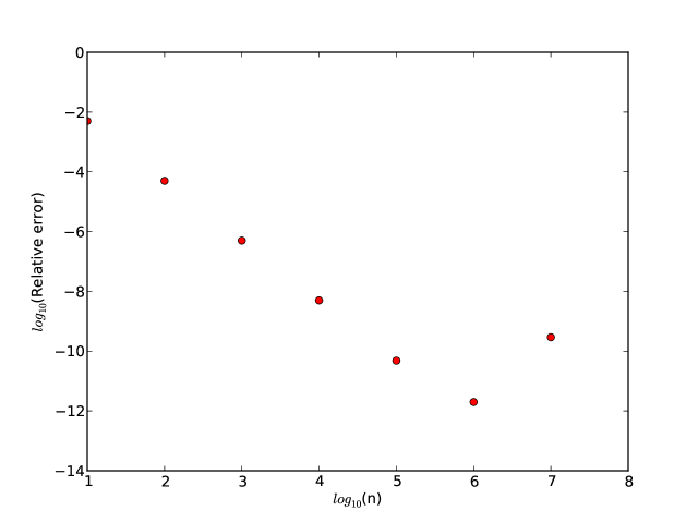
Figure 1: Log-log plot of the relative error as function of the number of integration points. Till approximately $n=10^{6}$, the relative error follows the predicted mathematical error of the trapezoidal rule. For higher numbers of integration points, numerical round off errors and loss of numerical precision give an increasing relative error.

The above example allows the student to also test the mathematical error of the algorithm for the trapezoidal rule by changing the number of integration points. The students get trained from day one to think error analysis. Figure 1 shows clearly the region where the relative error starts increasing. The mathematical error which follows the trapezoidal rule goes as $O(h^{2})$ where $h$ is the chosen numerical step size. It is proportional to the inverse of the number of integration points $n$, that is $h\propto 1/n$.

Before numerical round-off errors and loss of numerical precision kick in (near $h\sim 10^{-6}$) we see that the relative error in the log-log plot has a slope which follows the mathematical error.

There are several additional benefits here. The general learning outcomes on computing can be included as in for example the following ways. We can easily bake in how to structure a code in terms of functions and modules, or how to read input data flexibly from the command line or how to write unit tests etc. The conventions and techniques outlined here will save students a lot of time when one extends incrementally software over time, from simpler to more complicated problems. In the next subsection we show how algorithms for solving sets of ordinary differential equations and finding eigenvalues can be reused in different courses with minor modifications only.

0.4.2 From Mathematics to Physics

We assume that our students know how to solve and study systems of ordinary differential with initial conditions only. Later in this section we will venture into two-point boundary value problems that can be studied and solved with eigenvalue solvers.

Let us start with initial value problems and ordinary differential equations. Such equations appear in a wealth of physics applications. Typical examples students will encounter are the classical pendulum in a mechanics course, an RLC circuit in the course on electromagnetism, the modeling of the Solar system in an Astrophysics course and many other cases. The essential message is that, with properly scaled equations, students can use essentially the same algorithms to solve these problems, either starting with a simple modified Euler algorithm or a Runge-Kutta class of algorithms or the so-called Verlet class of algorithms, to mention a few.

The idea is that algorithms students develop and use in one course can be reused in other courses. This allows students to make the relevant abstractions discussed above, opening up for a much wider range of applicabilities.

Here we look at two familiar cases from mechanics and electromagnetism, the equations for the classical pendulum and those for an RLC circuit. When properly scaled, these equations are essentially the same. To scale equations, either in terms of dimensionless variables or appropriate variables, is an important aspect which allows the students to see the potential for abstractions and hopefully see how the problems studied in say a mechanics course can be transferred to other fields.

The classical pendulum with damping and external force as it could appear in a mechanics course is given by the following equation of motion for the angle $\theta$ as function of time $t$

$$ml\frac{d^{2}\theta}{dt^{2}}+\nu\frac{d\theta}{dt}+mgsin(\theta)=Acos(\omega t),$$

where $m$ is its mass, $l$ the length, $\nu$ a damping factor and $A$ the amplitude of an applied external source with frequency $\omega$. The solution of this type of equations (second-order differential equations with given initial conditions) is something the students encounter the first semester thorugh the courses IN1900 and MAT-INF1100 at the University of Oslo. At Michigan State University there is now a compulsory course for physics majors that includes many of these elements. With this background, students are already familiar with the numerical solution and visualization of such equations. If we now move to a course on electromagnetism, we encounter almost the same equation for an RLC circuit, namely

$$L\frac{d^{2}Q}{dt^{2}}+\frac{Q}{C}+R\frac{dQ}{dt}=Acos(\omega t),$$

where $L$ is the inductance, $R$ the applied resistance, $Q$ the time-dependent charge and $C$ the capacitance.

Let us consider first the classical pendulum equations with damping and an external force and define the scaled velocity $\hat{v}$ as

$$\frac{d\theta}{d\hat{t}}=\hat{v},$$

where we have defined a dimensionless time variable $\hat{t}$. With the equation for the velocity we can rewrite the second-order differential in terms of two coupled first-order differential equations where the second equation represents the acceleration

$$\frac{d\hat{v}}{d\hat{t}}=Acos(\hat{\omega}\hat{t})-\hat{v}\xi-\sin(\theta).$$

We have scaled the equations with $\omega_{0}=\sqrt{g/l}$, $\hat{t}=\omega_{0}t$ and $\xi=mg/\omega_{0}\nu$. The frequency $\omega_{0}$ defines a so-called natural frequency defined by the gravitational acceleration $g$ and the length of the pendulum $l$. The frequency $\hat{\omega}=\omega/\omega_{0}$. In a similar way, our RLC circuit can now be rewritten in terms of two coupled first-order differential equations,

$$\frac{dQ}{d\hat{t}}=\hat{I},$$

and

$$\frac{d\hat{I}}{d\hat{t}}=Acos(\hat{\omega}\hat{t})-\hat{I}\xi-Q,$$

with $\omega_{0}=1/\sqrt{LC}$, $\hat{t}=\omega_{0}t$ and $\xi=CR\omega_{0}$. Here we see that the natural frequency is defined in terms of the physical parameters $L$ and $C$.

The equations are essentially the same, the main differences reside in the different scaling constants and the introduction of a non-linear term for the angle $\theta$ in the pendulum equation. The differential solver the students end up writing in the mechanics course (which comes normally before the course on electromagnetism) can then be reused in the electromagnetism course, with a great potential for further abstraction.

Let us now move to another frequently encountered problem in several physics courses, namely that of a two-point boundary value problem. In the examples below we will see again that if the equations are properly scaled, we can reuse the same algorithm for solving different physics problems. Here we will start with the equations for a buckling beam (a case which can be found in a mechanics course or a course on mathematical methods in physics). Thereafter, with a simple change of variables and constants, the same problem can be used to study a quantum mechanical particle confined to move in an infinite potential well. By simply changing the diagonal matrix elements of the discretized differential equation problem, we can study particles that move in a harmonic oscillator potential or other types of quantum-mechanical one-body or selected two-body problems. With slight modifications to the matrix that results from the discretization of a second derivative, we can study Poisson’s equation in one dimension, a problem of relevance in electromagnetism.

Let us start with the buckling beam. This is a two-point boundary value problem

$$R\frac{d^{2}u(x)}{dx^{2}}=-Fu(x),$$

where $u(x)$ is the vertical displacement, $R$ is a material specific constant, $F$ is the applied force and $x\in[0,L]$ with $u(0)=u(L)=0$. We scale the equation with $x=\rho L$ and $\rho\in[0,1]$ and get (note that we change from $u(x)$ to $v(\rho)$)

$$\frac{d^{2}v(\rho)}{dx^{2}}+Kv(\rho)=0,$$

which is, when discretized (see below), nothing but a standard eigenvalue problem with $K=FL^{2}/R$. Here we can assume that either the force $F$ or the material specific rigidity $R$ are unknown. If we replace $R=-\hbar^{2}/2m$ and $-F=\lambda$, we have the quantum mechanical variant for a particle moving in a well with infinite walls at the endpoints. The way to solve these equations numerically is to discretize the second derivative and the right hand side as

$$-\frac{v_{i+1}-2v_{i}+v_{i-i}}{h^{2}}=\lambda v_{i},$$

with $i=1,2,\dots,n$. Here $h$ is the step size which is defined by the number of integration (or mesh) points. We need to add to this system the two boundary conditions $v(0)=v_{0}$ and $v(1)=v_{n+1}$, although they are not needed in the solution of the equations since their values are known. For all integration points $i=1,2,\dots,n$ the set of equations to solve result in a so-called tridiagonal Toeplitz matrix ( a special case from the discretized second derivative)

$$\mathbf{A}=\frac{1}{h^{2}}\begin{bmatrix}2&-1&&&&\\ -1&2&-1&&&\\ &-1&2&-1&&\\ &\dots&\dots&\dots&\dots&\dots\\ &&&-1&2&-1\\ &&&&-1&2\\ \end{bmatrix}$$

and with the corresponding vectors $\mathbf{v}=(v_{1},v_{2},\dots,v_{n})^{T}$ allows us to rewrite the differential equation as a standard eigenvalue problem

$$\mathbf{A}\mathbf{v}=\lambda\mathbf{v}.$$

The tridiagonal Toeplitz matrix has analytical eigenpairs, providing us thereby with an invaluable check on the equations to be solved.

If we stay with quantum mechanical one-body problems (or special interacting two-body problems) adding a potential along the diagonal elements allows us to reuse this problem for many types of physics cases. To see this, let us assume we are interested in the solution of the radial part of Schrödinger’s equation for one electron. This equation reads

$$-\frac{\hbar^{2}}{2m}\left(\frac{1}{r^{2}}\frac{d}{dr}r^{2}\frac{d}{dr}-\frac{l(l+1)}{r^{2}}\right)R(r)+V(r)R(r)=ER(r).$$

Suppose in our case $V(r)$ is the harmonic oscillator potential $(1/2)kr^{2}$ with $k=m\omega^{2}$ and $E$ is the energy of the harmonic oscillator in three dimensions. The oscillator frequency is $\omega$ and the energies are

$$E_{nl}=\hbar\omega\left(2n+l+\frac{3}{2}\right),$$

with $n=0,1,2,\dots$ and $l=0,1,2,\dots$.

Since we have made a transformation to spherical coordinates it means that $r\in[0,\infty)$. The quantum number $l$ is the orbital momentum of the electron. In order to find analytical solutions for this problem, we would substitute $R(r)=(1/r)u(r)$ (which gives $u(0)=u(\infty)=0$ and thereby easier boundary conditions) and obtain

$$-\frac{\hbar^{2}}{2m}\frac{d^{2}}{dr^{2}}u(r)+\left(V(r)+\frac{l(l+1)}{r^{2}}\frac{\hbar^{2}}{2m}\right)u(r)=Eu(r).$$

The boundary conditions are $u(0)=0$ and $u(\infty)=0$.

In order to scale the equations, we introduce a dimensionless variable $\rho=(1/\alpha)r$ where $\alpha$ is a constant with dimension length and get

$$-\frac{\hbar^{2}}{2m\alpha^{2}}\frac{d^{2}}{d\rho^{2}}v(\rho)+\left(V(\rho)+\frac{l(l+1)}{\rho^{2}}\frac{\hbar^{2}}{2m\alpha^{2}}\right)v(\rho)=Ev(\rho).$$

Let us choose $l=0$ for the mere sake of simplicity. Inserting $V(\rho)=(1/2)k\alpha^{2}\rho^{2}$ we end up with

$$-\frac{\hbar^{2}}{2m\alpha^{2}}\frac{d^{2}}{d\rho^{2}}v(\rho)+\frac{k}{2}\alpha^{2}\rho^{2}v(\rho)=Ev(\rho).$$

We multiply thereafter with $2m\alpha^{2}/\hbar^{2}$ on both sides and obtain

$$-\frac{d^{2}}{d\rho^{2}}v(\rho)+\frac{mk}{\hbar^{2}}\alpha^{4}\rho^{2}v(\rho)=\frac{2m\alpha^{2}}{\hbar^{2}}Ev(\rho).$$

A natural length scale comes out automatically when scaling. To see this, since $\alpha$ is constant we are left to determine, we determine $\alpha$ by requiring that

$$\frac{mk}{\hbar^{2}}\alpha^{4}=1.$$

This defines a natural length scale in terms of the various physical constants that determine the equation. The final expression, inserting $k=m\omega^{2}$ is

$$\alpha=\left(\frac{\hbar}{m\omega}\right)^{1/2}.$$

If we were to replace the harmonic oscillator potential with the attractive Coulomb interaction from the hydrogen atom, the parameter $\alpha$ would equal the Bohr radius $a_{0}$. This way students see the general properties of a two-point boundary value problem and can reuse the code they developed for a mechanics course to the subsequent quantum mechanical course.

Defining

$$\lambda=\frac{2m\alpha^{2}}{\hbar^{2}}E,$$

we can rewrite Schroedinger’s equation as

$$-\frac{d^{2}}{d\rho^{2}}v(\rho)+\rho^{2}v(\rho)=\lambda v(\rho).$$

This is similar to the equation for a buckling beam, except for the potential term. In three dimensions with our scaling, the eigenvalues for $l=0$ are $\lambda_{0}=3,\lambda_{1}=7,\lambda_{2}=11,\dots.$

If we define first the diagonal matrix element

$$d_{i}=\frac{2}{h^{2}}+V_{i},$$

and the non-diagonal matrix element

$$e_{i}=-\frac{1}{h^{2}},$$

we can rewrite the Schröedinger equation as

$$d_{i}u_{i}+e_{i-1}v_{i-1}+e_{i+1}v_{i+1}=\lambda v_{i},$$

where $v_{i}$ is unknown and $i=1,2,\dots,n$. We can reformulate the latter equation as a matrix eigenvalue problem

$$\begin{bmatrix}d_{1}&e_{1}&0&0&\dots&0&0\\ e_{1}&d_{2}&e_{2}&0&\dots&0&0\\ 0&e_{2}&d_{3}&e_{3}&0&\dots&0\\ \dots&\dots&\dots&\dots&\dots&\dots&\dots\\ 0&\dots&\dots&\dots&\dots&d_{n-1}&e_{n-1}\\ 0&\dots&\dots&\dots&\dots&e_{n-1}&d_{n}\end{bmatrix}\begin{bmatrix}v_{1}\\ v_{2}\\ \dots\\ \dots\\ \dots\\ v_{n}\end{bmatrix}=\lambda\begin{bmatrix}{c}v_{1}\\ v_{2}\\ \dots\\ \dots\\ \dots\\ v_{n}\end{bmatrix}$$

or if we wish to be more detailed, we can write the tridiagonal matrix as

$$\begin{bmatrix}\frac{2}{h^{2}}+V_{1}&-\frac{1}{h^{2}}&0&0&\dots&0&0\\ -\frac{1}{h^{2}}&\frac{2}{h^{2}}+V_{2}&-\frac{1}{h^{2}}&0&\dots&0&0\\ 0&-\frac{1}{h^{2}}&\frac{2}{h^{2}}+V_{3}&-\frac{1}{h^{2}}&0&\dots&0\\ \dots&\dots&\dots&\dots&\dots&\dots&\dots\\ 0&\dots&\dots&\dots&\dots&\frac{2}{h^{2}}+V_{n-1}&-\frac{1}{h^{2}}\\ 0&\dots&\dots&\dots&\dots&-\frac{1}{h^{2}}&\frac{2}{h^{2}}+V_{n}\end{bmatrix}.$$

The following Python code sets up the matrix to diagonalize by defining the minimun and maximum values of $r$ with a maximum value of integration points. It plots the eigenfunctions of the three lowest eigenstates.

⬇

#Program which solves the one-particle Schrodinger equation

#for a potential specified in function

#potential().

from matplotlib import pyplot as plt

import numpy as np

#Function for initialization of parameters

def initialize():

RMin = 0.0

RMax = 10.0

lOrbital = 0

Dim = 400

return RMin, RMax, lOrbital, Dim

# Harmonic oscillator potential

def potential(r):

return 0.5*r*r

#Get the boundary, orbital momentum and number of integration points

RMin, RMax, lOrbital, Dim = initialize()

#Initialize constants

Step = RMax/(Dim)

DiagConst = 2.0/ (Step*Step)

NondiagConst = -1.0 / (Step*Step)

OrbitalFactor = lOrbital * (lOrbital + 1.0)

#Calculate array of potential values

v = np.zeros(Dim)

r = np.linspace(RMin,RMax,Dim)

for i in range(Dim):

r[i] = RMin + (i+1) * Step;

v[i] = potential(r[i]) + OrbitalFactor/(r[i]*r[i]);

#Setting up a tridiagonal matrix and finding eigenvectors and eigenvalues

Matrix = np.zeros((Dim,Dim))

Matrix[0,0] = DiagConst + v[0];

Matrix[0,1] = NondiagConst;

for i in xrange(1,Dim-1):

Matrix[i,i-1] = NondiagConst;

Matrix[i,i] = DiagConst + v[i];

Matrix[i,i+1] = NondiagConst;

Matrix[Dim-1,Dim-2] = NondiagConst;

Matrix[Dim-1,Dim-1] = DiagConst + v[Dim-1];

# diagonalize and obtain eigenvalues, not necessarily sorted

EigValues, EigVectors = np.linalg.eig(Matrix)

# sort eigenvectors and eigenvalues

permute = EigValues.argsort()

EigValues = EigValues[permute]

EigVectors = EigVectors[:,permute]

# now plot the results for the three lowest lying eigenstates

for i in range(3):

print(EigValues[i])

FirstEigvector = EigVectors[:,0]

SecondEigvector = EigVectors[:,1]

ThirdEigvector = EigVectors[:,2]

plt.plot(r, FirstEigvector**2 ,'b-',r, SecondEigvector**2 ,'g-',r, ThirdEigvector**2 ,'r-')

plt.axis([0,4.6,0.0, 0.025])

plt.xlabel(r'$r$')

plt.ylabel(r'Radial probability $r^2|R(r)|^2$')

plt.title(r'Radial probability distributions for three lowest-lying states')

plt.savefig('eigenvector.pdf')

plt.show()

The last example shows the potential of combining numerical algorithms with analytical results (or eventually symbolic calculations), allowing thereby students to test their physics understanding. One can easily switch to other potentials by simply redefining the potential function. For example, a finite box potential can easily be defined as

⬇

# Finite depth and range box potential, with strength V and range a

def potential(r):

if r >= 0.0 and r <= 10.0:

V = -0.05

else:

V =0.0

return V

Thereafter, the students can explore the role of the potential depth and the range of the potential. Analyzing the eigenvectors gives additional information about the spatial degrees of freedom in terms of different potentials. The possibility to visualize the results immediately, as shown in figure 2, aids in providing students with a deeper understanding of the relevant physics.

This example contains also many of the computing learning outcomes we discussed above, in addition to those related to the physics of a particular system. We see that, by proper scaling, the students can make further abstractions and explore other physics cases easily where no analytical solutions are known. With unit testing and analytical results they can validate and verify their algorithms.

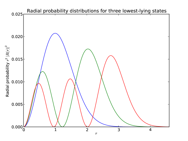
Figure 2: Plot of the eigenfunctions of the three lowest-lying eigenvalues for a harmonic oscillator problem in three dimensions. The students can easily change the type of potential and explore the physics that arises from these potentials.

The above example allows the student to test the mathematical error of the algorithm for the eigenvalue solver by simply changing the number of integration points. Again, as discussed above in connection with the trapezoidal rule, the students get trained to develop an understanding of the error analysis and where things can go wrong. The algorithm can be tailored to any kind of one-particle problem used in quantum mechanics.

A simple rewrite allows for the reuse in linear algebra problems for solution of say Poisson’s equation in electromagnetism, or the diffusion equation in one dimension. To see this and how the same matrix can be used in a course in electromagnetism, let us consider Poisson’s equation. We assume that the electrostatic potential $\Phi$ is generated by a localized charge distribution $\rho(\mathbf{r})$. In three dimensions the pertinent equation reads

$$\nabla^{2}\Phi=-4\pi\rho(\mathbf{r}).$$

With a spherically symmetric potential $\Phi$ and charge distribution $\rho(\mathbf{r})$ and using spherical coordinates, the relevant equation to solve simplifies to a one-dimensional equation in $r$, namely

$$\frac{1}{r^{2}}\frac{d}{dr}\left(r^{2}\frac{d\Phi}{dr}\right)=-4\pi\rho(r),$$

which can be rewritten via a substitution $\Phi(r)=\phi(r)/r$ as

$$\frac{d^{2}\phi}{dr^{2}}=-4\pi r\rho(r).$$

The inhomogeneous term $f$ or source term is given by the charge distribution $\rho$ multiplied by $r$ and the constant $-4\pi$.

We can rewrite this equation by letting $\phi\rightarrow u$ and $r\rightarrow x$. Scaling again the equations and replacing the right hand side with a function $f(x)$, we can rewrite the equation as

$$-u^{\prime\prime}(x)=f(x).$$

Our scaling gives us again $x\in[0,1]$ and the two-point boundary value problem with $u(0)=u(1)=0$. With $n+1$ integration points and the step length defined as $h=1/(n)$ and replacing the continuous function $u$ with its discretized version $v$, we get the following equation

$$-\frac{v_{i+1}+v_{i-1}-2v_{i}}{h^{2}}=f_{i}\hskip 14.22636pt\mathrm{for}\hskip 2.84544pti=1,\dots,n,$$

where $f_{i}=f(x_{i})$. Bringing up again the tridiagonal Toeplitz matrix,

$$\mathbf{A}=\frac{1}{h^{2}}\begin{bmatrix}2&-1&0&\dots&\dots&0\\ -1&2&-1&0&\dots&\dots\\ 0&-1&2&-1&0&\dots\\ &\dots&\dots&\dots&\dots&\dots\\ 0&\dots&&-1&2&-1\\ 0&\dots&&0&-1&2\\ \end{bmatrix},$$

our problem becomes now a classical linear algebra problem

$$\mathbf{A}\mathbf{v}=\mathbf{f},$$

with the unknown function $\mathbf{v}$. Using standard LU decomposition algorithms GolubVanLoan (here one can use the so-called Thomas algorithm which reduces the number of floating point operations to $O(n)$) one can easily find the solution to this problem.

These examples demonstrate how one can, with a discretized second derivative, solve physics problems that arise in different undergraduate courses using standard linear algebra and eigenvalue algorithms and ordinary differential equations, allowing thereby teachers to focus on the interesting physics. Many of these problems can easily be linked up with ongoing research. This opens up for many interesting perspectives in physics education. We can bring in at a much earlier stage in our education basic research elements and perhaps even link with ongoing research during the first year of undergraduate studies.

Instead of focusing on tricks and mathematical manipulations to solve the continuous problems for those few case where an analytical solution can be found, the discretization of the continuous problem opens up for studies of many more interesting and realistic problems. However, we have seen that in order to verify and validate our codes, the existence of analytical solutions offer us an invaluable test of our algorithms and programs. The analytical results can either be included explicitely or via symbolic software like Python’s Sympy package. Thus, computing stands indeed for solving scientific problems using all possible tools, including symbolic computing, computers and numerical algorithms, numerical experiments (as well as real experiments if possible) and analytical paper and pencil solutions.

The cases we have presented here represent only a limited set of examples. A longer version of this article, with more examples and details on assessments programs, is under preparation as a textbook DannyMortenBook . The possible learning outcomes we defined for various physics courses are often based on the above simple discretization. With basic knowledge on how to solve linear algebra problems, eigenvalue porblems and differential equations, topics normally taught in mathematics and computational science courses, we can offer our students a much more challenging and interesting education. Furthermore, we give our students the competencies which are required by future employers, either in the private or the public sector.

0.5 Conclusions and Perspectives

In this contribution, we have outlined some of the basic elements that we feel are necessary to address in order to introduce computing in various undergraduate physics courses. Some of the conclusions we would like to emphasize include a proper definition of computing, the development of learning outcomes that apply to both computational science, mathematics, and physics courses as well as proper assessment programs.

Collaboration across departments is necessary in order to achieve a synchronization between various topics and learning outcomes, as well as an early introduction to programming. Many universities require such courses as part of a physics degree. Coordinating such a programming course with mathematics courses and other science courses results in a better coordination of both learning outcomes and computing skills and abilities. The experiences we have drawn from the University of Oslo and Michigan State University show that an early and compulsory programming course, which includes central scientific elements, is important in order to integrate properly a computational perspective in our physics education.

The benefits are many, in particular it allows us to make our research more visible in early undergraduate physics courses, enhancing research-based teaching with the possibility to focus more on understanding and increased insight. It gives also our candidates the skills and abilities that are requested by society at large, both from the private and the public sectors. With computing, we emphasize a broader and more up-to-date education with a problem-based orientation, often requested by potential employers. Furthermore, our experiences from the both universities indicate that a discussion of computing across disciplines results in an increased impetus for broad cooperation in teaching and a broader focus on university pedagogical topics.

We are now in the process of developing computing learning outcomes with examples for central physics courses. Together with a research based assessment program, we will be able to answer central questions like whether the introduction of computing increases a student’s insights and understanding of the underlying physics.

- (1) Association for Computing Machinery, 2013, {http://pathways.acm.org/executive-summary.html}.
- (2) Computing in Science Education project, University of Oslo, Norway, https://www.mn.uio.no/english/about/collaboration/cse/.
- (3) Center for Computing in Science Education, University of Oslo, Norway, {http://www.mn.uio.no/ccse/english/}.
- (4) Marcos Daniel Caballero and Morten Hjorth-Jensen, Integrating a Computational Perspective in Physics Courses, in preparation.
- (5) Partnership for Integration of Computation into Undergraduate Physics, {http://www.compadre.org/picup/}PICUP project.
- (6) Physics Education Research Group at Michigan State University, https://perl.natsci.msu.edu/.
- (7) Anders Malthe-Sørenssen, Elementary Mechanics Using Python, Undergraduate Lecture Notes in Physics (Springer, Berlin, 2015).
- (8) Arnt Inge Vistnes, Waves and Motion, in press, Undergraduate Texts in Physics (Springer, Berlin, 2018).
- (9) Anders Malthe-Sørenssen and Dag Kristian Dysthe, Statistical and Thermal Physics, in press, Undergraduate Texts in Physics (Springer, Berlin, 2018/2019).
- (10) Symbolic Python, .
- (11) Gene H. Golub and Charles F. Van Loan, Matrix Computations (The Johns Hopkins University Press, 1996, Baltimore and London).