Results from The Latin American Giant Observatory Space Weather Simulation Chain
Abstract
The Space Weather program of the Latin American Giant Observatory (LAGO) Collaboration was designed to study the variation of the flux of atmospheric secondary particles at ground level produced during the interaction of cosmic rays with the air. This work complements and expands the inference capabilities of the LAGO detection network to identify the influence of solar activity on the particle flux, at places having different geomagnetic rigidity cut-offs and atmospheric depths. This program is developed through a series of Monte Carlo sequential simulations to compute the intensity spectrum of the various components of the radiation field on the ground. A key feature of these calculations is that we performed detailed radiation transport computations as a function of incident direction, time, altitude, as well as latitude and longitude. Magnetic rigidity calculations and corrections for geomagnetic field activity are established by using the MAGNETOCOSMICS code, and the estimation of the flux of secondaries at ground level is implemented by using the CORSIKA code; thus we can examine the local peculiarities in the penumbral regions with a more realistic description of the atmospheric and geomagnetic response in these complex regions of the rigidity space. As an example of our calculation scheme, we report some result on the flux at ground level for two LAGO locations: Bucaramanga-Colombia and San Carlos de Bariloche-Argentina, for the geomagnetically active period of May 2005.
Laboratorio Detección de Partículas y Radiación (CNEA,CONICET,UNCUYO), San Carlos de Bariloche, Argentina.
Instituto de Tecnologías en Detección y Astropartículas (CNEA,CONICET,UNSAM), Buenos Aires, Argentina.
Escuela de Física, Universidad Industrial de Santander, 680002 Bucaramanga, Colombia.
Departamento de Física, Universidad de Los Andes 5101 Mérida, Venezuela.
M. Suárez-Durán mauricio.suarez@correo.uis.edu.co
An extended rigidity cutoff is calculated under quiet (secular) & transient conditions for the geomagnetic field.
Penumbra region is reinterpreted as a probability function of the arrival direction.
The effect of the geomagnetic field in the flux of Galactic Cosmic Rays can be estimated from changes on the flux of secondary particles at ground level.
1 Introduction
Solar activity has a strong influence on the modulation of the flux of galactic cosmic rays (GCRs) arriving at Earth, whose transport through the heliosphere is one of the topics of major interest in space physics, presenting several unresolved questions. Space weather physics is experiencing a fast growing interest nowadays because of evidence that environmental conditions in the near-Earth space have direct and indirect impacts on technology and the global economy (Schrijver et al., 2015).
One of most puzzling modulation of the cosmic rays flux at ground level is called Forbush Decrease (FD): a rapid reduction in the observed galactic cosmic ray intensity followed by a slow exponential-like recovery (Usoskin et al., 2008). This phenomenon initially was reported by S.E. Forbush –and almost simultaneously by V.F. Hess & A. Demmelmair– in 1937 (see e.g. Forbush, 1937; Hess and Demmelmair, 1937). Later, in the 1950’s, the works of Simpson, Fonger & Treiman (Simpson et al., 1953), and Singer (Singer, 1954), showed that FDs are related to the solar activity interacting with the interplanetary medium. More recently, Lockwood showed a dependence of the magnitude of the FD upon the vertical cutoff rigidity (Lockwood, 1971).
FDs can be classified in two groups: recurrent and non-recurrent FD. While the first group (Lockwood, 1971) have a symmetric profile and are well associated with co-rotating high speed solar wind streams (Cane, 2000), non-recurrents FD have sudden onsets with a maximum depression within a day, and a more gradual recovery (Cane, 2000; Belov et al., 2014) , and are related to the interaction of GCRs, Interplanetary Coronal Mass Ejections (ICME) and a perturbed geomagnetic field (it is perturbed by its interaction with the same ICME).
Understanding these very complex phenomena depends upon: in situ measurements of the interaction of GCRs-ICME; tracking the propagation of GCRs through the Geomagnetic Field (GF hereafter); taking into account their interaction with the atmosphere, and also the variation of the particles produced by the latter interaction (hereafter secondaries) at ground level.
As the secondaries are produced by the interaction of GCRs with the atmosphere (hereafter denoted as primaries), the modulation of secondary particles needs to be monitored and carefully corrected by taking into account several atmospheric factors that could modify the flux of secondaries at Earth’s surface (the Atmospheric density profile is one of those factors because this is proportional to the absorption of secondaries particles) (The Pierre Auger Collaboration, 2011; Dasso et al., 2012; H. Asorey for the LAGO Collaboration, 2013; The Pierre Auger Collaboration, 2015; H. Asorey and S. Dasso and L. A. Núñez and Y. Pérez and C. Sarmiento-Cano and M. Suárez-Durán for the LAGO Collaboration, 2015). Furthermore, a series of completed and detailed simulations are needed to characterize the expected flux at the detector altitude. This kind of simulation must take into account several important factors such as GF conditions, i.e., estimations of the magnetic rigidity of the GCRs, the interaction of GCRs with atmosphere, the variations in atmospheric depth and the detector response.
Direct solar wind observations using spacecraft can provide insight of the interplanetary magnetic field; but its global structure can not be completely monitored by on-board measurements, because they can only detect local variations along the trajectory of the probe within the solar wind. On the other hand, ground observatories with detectors spread on very large areas, registering indirectly low energy GCRs, can provide important, alternative and complementary information about the broader structure of the interplanetary magnetic fields and its influence on the GCRs flux. In this context, a global network of both type of observatories combines different techniques to monitor the development of FDs at different geomagnetic latitudes and rigidity cutoffs, will enrich future studies on the detection of solar modulation of GCRs (see e.g. Abbasi et al., 2008; The Pierre Auger Collaboration, 2015).
The Latin American Giant Observatory (LAGO) (Allard et al., 2008; Asorey et al., 2015) has developed a program to understand the influence of the space weather phenomena on the flux of GCRs. This program, called LAGO Space Weather (LAGO-SW) (H. Asorey for the LAGO Collaboration, 2013), includes a precise simulation that takes into account the geomagnetic corrections and a detailed measurement of the modulation on the flux of secondaries, and evaluates if this modulation have possible causal correlations with space weather phenomena, like FDs (H. Asorey and S. Dasso and L. A. Núñez and Y. Pérez and C. Sarmiento-Cano and M. Suárez-Durán for the LAGO Collaboration, 2015).
Nowadays, computational capabilities allow the extension of the usual approach, which is to consider only the components of the GCR flux locally and include geomagnetic effects by an effective rigidity cutoff for vertical primaries (Masías-Meza and Dasso, 2014). The detailed simulations described in this work, include these effects over different arrival directions during dynamic events affecting the geomagnetic field and atmospheric conditions. We have generalized previous attempts by including not only secular, but also transient variations of the directional geomagnetic rigidity cutoff.
This paper is organized as follows: in section 2, the Latin American Giant Observatory and its space weather program are briefly described; then, in Section 3, we present our space weather simulation chain, focusing on geomagnetic corrections of the primary flux; in Section 4 we discuss our main results in secular conditions and later under geomagnetic disturbances for two LAGO sites: Bucaramanga-Colombia and San Carlos de Bariloche-Argentina. Finally, in section 5 some finals remarks and future projects are considered.
2 The LAGO Space Weather Program
The Latin American Giant Observatory (LAGO) is an extended astroparticle observatory on a continental scale, promoting training and research in astroparticle physics in Latin America covering three main areas: search for the high energy component of gamma rays bursts (GRBs) at high altitude sites, space weather phenomena, and background radiation at ground level (Asorey et al., 2015).
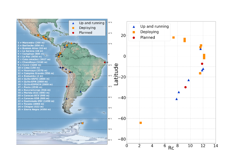
The LAGO detection network consists of ground-level water-Cherenkov particle detectors (WCDs), spanning over several sites, located at significantly different latitudes and various altitudes –from Mexico to the Patagonia and from mean sea level up to more than 5000 meters of altitude. After the installation of new detectors at the Antarctica Peninsula (Dasso et al., 2015), LAGO will cover a large range of geomagnetic rigidity cutoffs and atmospheric absorption/depths (I. Sidelnik for the LAGO Collaboration, 2015). The current/planned distribution and status of the LAGO detection network is shown in Figure 1. This network of detectors is operated by the LAGO Collaboration: a non-centralized and distributed collaborative network of more than 80 scientists from institutions of te Latin American countries (Argentina, Bolivia, Brazil, Chile, Colombia, Ecuador, Guatemala, Mexico, Peru and Venezuela) and Spain. The LAGO Collaboration is using WCDs in all sites, due to their proved reliability, high detection, low cost and efficiency of the detection of all components present in atmospheric extensive showers (Asorey et al., 2015; I. Sidelnik for the LAGO Collaboration, 2015; A. Galindo for the LAGO Collaboration, 2015; Dasso et al., 2015).
As explained in Asorey et al. (2015), the LAGO scientific and academic objectives are organized in different programs. The Space Weather LAGO Program is devised to study variations in the flux of secondary particles at ground level and its relation to the heliospheric modulation of GCRs. The LAGO detector network determines the flux of secondary particles in different bands of deposited energy in the detector, by using pulse shape discrimination techniques. This is what we have called the multi-spectral analysis technique (H. Asorey and S. Dasso and L. A. Núñez and Y. Pérez and C. Sarmiento-Cano and M. Suárez-Durán for the LAGO Collaboration, 2015). The total energy threshold for the detection of secondary particles are MeV for gammas, MeV for electrons and MeV for muons.
By combining all the data measured at different locations, LAGO provides simultaneous and detailed information of the temporal evolution of the secondary flux at different geomagnetic locations. This can help to get a better understanding of the small and large spacetime scales of the disturbances produced by different space weather phenomena (H. Asorey and S. Dasso and L. A. Núñez and Y. Pérez and C. Sarmiento-Cano and M. Suárez-Durán for the LAGO Collaboration, 2015).
Any attempt to estimate the expected flux of secondaries at any detector of the LAGO network should be based on a detailed simulation that takes into account all possible sources of flux variation. This complex approach comprises processes occurring at different spatial and time scales, following this conceptual scheme:
| GCR Flux | Modulated Flux | Primaries | ||
|---|---|---|---|---|
| Primaries | Secondaries | Signals. |
As it can be easily appreciated, the above simulation pipeline considers three important factors with different spatial and time scales: the geomagnetic effects, the development of the extensive air showers in the atmosphere, and the detector response at ground level. According to the above scheme, in this work we focused in stages covering from the modulated flux to the flux of secondary particles at ground level.
Our Simulation Chain can be depicted in three main consecutive blocks:
-
1.
The effects of GF on the propagation of charged particles, contributing to the background radiation at ground level, are characterized by the directional rigidity cutoff, , at each LAGO site and calculated using the MAGNETOCOSMICS code (Desorgher, 2004) applying the backtracking technique (see e.g. Masías-Meza and Dasso, 2014). The Geomagnetic Field at any point on Earth is determined by using the International Geomagnetic Field Reference, version 11 (International Association of Geomagnetism and Aeronomy, Working Group V-MOD, 2010) at the near-Earth GF () – distance from Earth center and is the Earth radius ( km)– and through the Tsyganenko Magnetic Field model version 2001 (TSY01 hereafter) (Tsyganenko, 2002) to describe the outer GF ().
-
2.
The second step of the chain is based on the CORSIKA code (Heck et al., 1998). Extensive air showers produced during the interaction of cosmic rays with the atmosphere are simulated with extreme detail to obtain a very comprehensive set of secondaries at ground level.
- 3.
3 The space weather simulation chain
The propagation of charged particle through the GF has been studied since the 60s and was focused on understanding how the penumbra region changes with the geographical position (see e.g. Shea et al., 1965; Carmichael et al., 1969; Smart and Shea, 2012). In this section we shall discuss our novel approach to understand the penumbra region and our proposal for a new method to calculate the magnetic rigidity as a function of time. We shall also describe in detail how geomagnetic effects on the low energy flux of primaries can be infered from observations of secondary particles at ground level by means of the following procedure:
-
1.
To find a magnetic rigidity function, , at a particular geographical position –i.e. latitude (Lat), longitude (Lon) and altitude above sea level (Alt)–, time () and arrival direction of the particle –i.e. zenithal () and azimuthal () angle;
-
2.
To calculate the flux of primaries at the top of the atmosphere ( km a.s.l. (Above Sea Level)), filtered by the magnetic rigidity function ;
-
3.
To estimate the flux of secondaries at ground level produced by the interactions of the impinging GCRs with the atmosphere.
The following subsections will develop all details for the above-mentioned actions.
3.1 Magnetic rigidity as function of time
The direction of the velocity of a GCR () changes along the particle trajectory inside the dynamic GF, , according to the equation
| (1) |
where is the path length along the particle trajectory and the magnetic rigidity; with as the particle momentum, the light speed, the atomic number and the electric charge of the electron. The variation of is weighted by and therefore a GCR is able to arrive at some specific geographical point –under some configuration of associated with the trajectory of the particle arriving to a particular position, i.e Latitude (), Longitude (), Altitude ()– if its has the right value. Thus, we can write as
| (2) |
Following standard definitions (see e.g. Cooke et al., 1991), particles with allowed will reach at certain geographical position, while those with forbidden will not. With these considerations, three different ranges of can be defined:
-
•
Forbidden range: a continuous range which goes from zero to the first allowed value of , say ;
-
•
Allowed range: cotaining all the rigidities above a certain value, say , for which all the rigidities containted in this range are allowed.
-
•
Penumbra range: the range () connecting the allowed and forbidden ranges.
The penumbra is characterized by a single, effective, rigidity value (Shea et al., 1965; Smart and Shea, 2009), which is used to establish whether a GCR arrives, or not, at the particular geographical point. This value is called the rigidity cutoff () and can be defined as
| (3) |
where is the resolution of the calculation. Strictly speaking, and depend on time, the arrival direction, the geographical position and the altitude; thus, we should consider that, at a geographical point,
| (4) |
It is important to note that definition (3) has the implicit assumption that all the particle trajectories have the same contribution in the penumbra region, i.e., the flat GCR spectrum approximation, according to (Dorman et al., 2008). In this approximation, the very complex problem of allowed trajectories in the penumbra region is simply replaced by an effective cutoff, only calculated for vertical primaries. We have refined this approximation by considering the penumbra not as a sharp cutoff, but as a relatively smooth transition between the forbidden and the allowed regions. In our approach, we extend the concept of the effective rigidity cutoff assuming that it can be approximated by a cumulative probability function (CDF).
The next subsection outlines the method we have implemented to calculate and to characterize the penumbra region as a cumulative probability function (CPF).
3.1.1 Magnetic Rigidity Calculation
We performed the calculation by the backtracking
technique (see e.g. Masías-Meza and Dasso, 2014), via the
MAGNETCOSMICS (MAGCOS) code, with a resolution of GV,
considering two conditions: secular and dynamic geomagnetic field
effects. For secular conditions we used the configuration of
the geomagnetic field on UTC April 26th 2005, because at
this time the registered Disturbance Storm Time Index (Dst index
hereafter,
https://www.ngdc.noaa.gov/stp/geomag/dst.html)
was zero with a variability of nT from 0 UTC of April
26th to 12 UTC of the same day
(http://wdc.kugi.kyoto-u.ac.jp/dst_final/200504/index.html).
For the dynamic GF contribution, we calculated the
according to the GF configuration for each hour of May 2005,
setting the parameters: Dynamic pressure, Dst index,
interplanetary magnetic fields components and , and
Tsyganenko’s parameters for model TSY01: G1 and G2(Tsyganenko, 2002).
These parameters were taken from the Virtual Radiation Belt Observatory (Weigel et al., 2009); values were calculated for zenith angles from to , with and azimuth angles (for each ) from to with , for both site.
3.1.2 Interpreting the Penumbra Region
Instead of the standard simplifying assumption for the penumbra region we build a cumulative probability function (CPF), valid from to , which replaces the usual concept of , (defined in equation (3)). We denote this CPF as , which represents the probabilty of the cosmic ray arriving at some geographical position with zenith angle , at time , with ; we take into account the following considerations:
-
•
the backtracking technique performed by MAGCOS is a deterministic method, which implies that it is not possible to calculate a statistical set of values for a specific arrival direction, i.e., pair of (,);
-
•
for each zenith angle we consider uniform ranges in azimuth with an angular amplitude of each one, i.e. for each zenith angle we have different penumbra regions; and
-
•
for each , the associated set of in the penumbra regions has a global minimal value ( hereafter) and a global maximum value ( hereafter).
Accordingly, it is possible to come up with a frequentist approach, assuming a probability function defined as:
| (5) |
where, for each , we have averaged over the azimuth angle, , within each penumbral range; the fraction of the number () of allowed values () over the total number of values calculated for the ’s set ().
Equation (5) implies that the domain interval for is
| (6) |
Thus, from (5) and (6) we define the cumulative distribution function for a GCR, arriving at the observation point with rigidity as
| (7) |
Notice that equation (7) implies that a GCR with has a probability of to arrive at the observation point through the zenith angle ; meanwhile a GCR with has probability to arrive at the same point with the same angle.
Currently, the usual is interpreted as a unique value in the penumbra region, which separates only two possibilities for an incoming particle with a zenith angle : arriving or not arriving. If a charged particle has a then it is considered to arrive at the geographical point, in the opposite case, if , it does not arrive. With our approach, it is clear that a GCR, with and zenith angle , can reach at the geographical point if , whereas with will not. But, if the belongs to the penumbra region, it does not meet any of the above criteria because is between 0 and 1. To set this value of in terms of arriving or not arriving, i.e., 0 or 1, we implement a Metropolis Monte Carlo algorithm as follows: for a value, different from and , we calculate a random number: . Then,
-
•
if , then ; otherwise
-
•
if , then .
Therefore, we interpret the rigidity cutoff as function of the cumulative distribution function, i.e.,
| (8) |
Now, from the dynamic magnetic rigidity definition we perform the same type of calculations but including the time () dependence, by evaluating equation (4) for different conditions at particular moments.
After applying the same procedure, we obtained the dynamic rigidity cut-off of a site, as
| (9) |
where represents the cumulative distribution function calculated under GF conditions at the moment , i.e.
| (10) |
At this point, we shall introduce three types of rigidity cut off labeled by three different indexes i.e, :
-
•
: for the standard definition of rigidity cutoff, i.e. equation (3).
- •
- •
With these two new types of rigidity cut-off, we shall redefine, in the next sections, several physical parameters associated with .
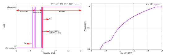
In the Figure 2, we show an example of the refinement for the estimation of the magnetic rigidity at Bucaramanga-Colombia, on May 13th 2005. In the left plot, we display the results of the standard method to calculate the rigidity cutoff (equation (3)). It is clear that even in those “not allowed zones” (between GeV and GeV) there are several trajectories that could contribute to the flux at the observation point. This could be particularly important when it is needed to determine the background flux at high altitude sites, such as the LAGO site of Mount Chacaltaya at m a.s.l., or even for the determination of the expected flux of secondaries impacting aircrafts (Pinilla et al., 2015; Asorey et al., 2017). In the same Figure 2 (right plot), we illustrate our new method, displaying for different magnetic rigidities, considering a primary with .
With our method in determining the local directional rigidity cutoff, it is possible to refine the calculation of the flux of particles at any observation point while taking into account GF disturbances, either in long time scales (secular conditions) on during short term transient phenomena.
3.2 Estimation of the Primary Flux filtered by
The second step in our simulation chain is to estimate GCR flux arriving at some geographical point ( km a.s.l., ) in the area , during time , in the solid angle – is the zenith angle– , within the energy interval and with minimum allowed primary momentum of
| (11) |
with the atomic number. Equation (11) allows us to filter primaries with insufficient to arrive at the point ().
We estimated the GCR flux, , at an altitude of km a.s.l., in accordance with the Linsley atmospheric model (NOAA, 1976); e.g. at this altitude the mass overburden vanishes (Heck et al., 1998), and we approximate by a simple power law of the form:
| (12) |
where the spectral index () can be considered constant with respect the energy, i.e. , from eV to eV (Letessier-Selvon and Stanev, 2011) and has a value of eV. For each type of GCR considered, , is individualized by its mass number (A) and atomic number (Z). Finally, is the normalization parameter. Both, the spectral indices and , have been obtained from the compilation produced by (Wiebel-Sooth et al., 1998).
We calculated using the fact that multiple observations have confirmed that at low energies ( eV) the GCR flux can be considered isotropic (see e.g. Abraham et al., 2007) and, in this case, equation (12) is integrated to obtain the expected number of primaries for every nuclei as:
| (13) |
with as the energy gap, which, in our case, varies from a few GeV () up to GeV () (Asorey, H. for The Pierre Auger Collaboration, 2011). It is clear that the first factor depends only on the zenith angle , and so, . Thus, equation (13) can be expressed as
| (14) |
where . For the calculation of we have used: m2, s, i.e., at least one day of the primary flux per square meter for each primary in the range , for from to . The will then be filtered via according to equation (11).
This means that we can identify three different kinds of primary fluxes, one per each different GF conditions :
-
•
for , i.e. .
-
•
for , i.e. .
-
•
for , i.e. .
Thus, the number of particles given by (14) will be susceptible to corrections by the modification of the local rigidity cutoff, and it can be re-written as
| (15) |
Here, the subindex of any quantity denotes the type of effect included.
As value of we have used GeV, because at these energies the flux is so low that it can not affect the distribution of the secondary background at ground level. It is important to stress that, for a given point, depends on the primary , theta arrival direction and time, i.e., .
3.3 Estimation of flux of secondary particles at ground level corrected by the Geomagnetic Field
The following step of the simulation chain is the correction for the effect of the Geomagnetic Field on the flux of secondary particles at ground level. As was mentioned in section 2, one of the main objectives of this simulation chain is to calculate the expected flux of secondaries at the detector level at any site of the LAGO network. Once the primary flux is calculated, the second step is to determine the interactions of those primaries with the atmosphere. This simulation step is performed with the CORSIKA code (Heck et al., 1998) (Currently, CORSIKA v7.3500, compiled using the following options: QGSJET-II-04 (Ostapchenko, 2011); GHEISHA-2002; EGS4; curved and external atmosphere, and volumetric detector). The local geomagnetic field values and needed by CORSIKA to account for GF effects during particles propagation in the atmosphere are obtained from the IGRF-11 model. Secondary particles are tracked to the lowest energy threshold allowed by CORSIKA for each type (currently, GeV for and hadrons (excluding ), and GeV for and ) to get the most comprehensive distribution of secondaries at each site. In this work, the atmosphere at each site was simulated by using profiles of the applicable MODTRAN atmospheric model (Kneizys et al., 1996) provided with CORSIKA. For the Bucaramanga site we use a tropical profile and for San Carlos de Bariloche a midlatitude summer profile. Currently, the LAGO collaboration is developing and validating a method to obtain the local atmospheric profiles for each LAGO site during different weather conditions based on the Global Data Assimilation System (GDAS) (NOAA, 2009), as differences have been observed between generic MODTRAN models and balloon measurements at the planed LAGO site in Antarctica (Dasso et al., 2015).
A large number of primary showers need to be simulated (typical values are of several billions of showers for 24 h of flux at each site). A set of local clusters have been deployed and tuned for this particular calculation. These are maintained at some institutions of the LAGO Collaboration. This simulation chain has been also integrated into a dedicated Virtual Organization, lagoproject, as part of the European Grid Infrastructure (EGI, http://www.egi.eu) activities. The Grid implementation of CORSIKA was deployed with two “flavors”, which run by using GridWay Metascheduler (http://www.gridway.org/doku.php) (Huedo et al., 2001) or with a second approach through a Catania Science Gateway interface (Barbera et al., 2011). Massive calculations can be executed with the former, via the Montera (Rodriguez-Pascual et al., 2013), the GWpilot (Rubio-Montero et al., 2015a) or the GWcloud (Rubio-Montero et al., 2015b) frameworks.
In the Science Gateway approach a user can seamlessly run a code on different infrastructures by accessing a unique web-based entry point with an identity provision. Users only have to upload the input data or invoke a PID (persistent identifier or reference to a digital set of files) and click on the run icon. The final result will be retrieved whenever the job has ended. The underlying infrastructure is absolutely transparent to the user and the system decides on which sites and computing platform the code will be compiled and run (Rodriguez-Pascual et al., 2015; Asorey et al., 2016).
To deal with the computational complexity introduced by the refinement described in the previous subsection, we built a library for each site containing the simulated particles starting from a very low momentum primary threshold of MeV (i.e. GeV of total energy for protons). Each secondary impinging the detector is tagged with information from its parent primary particle, which allows the calculation of its magnetic rigidity . Then, because each secondary at the ground comes from some primary impinging at the atmosphere, from the obtained for each condition according to equations (11) and (15), we are able to determine if each secondary would reach the detector under that particular GF condition.
4 Results for the LAGO sites of Bucaramanga, Colombia and San Carlos de Bariloche, Argentina
4.1 Magnetic Rigidity
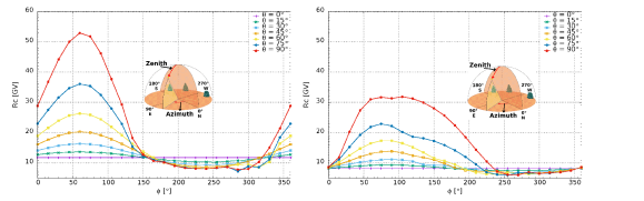
As we mentioned before, we applied our simulation chain to the location of two LAGO sites: Bucaramanga, Colombia (BGA) and San Carlos de Bariloche, Argentina (BRC). Results for the standard rigidity cutoff calculation, , are displayed in Figure 3 for each site. As expected, there is a strong dependence between and the arrival directions at both cities, which induces a noticeable decrease in the number of GCRs producing secondary particles at ground level. For Bucaramanga, it is interesting to mention the oddity of the behavior of the rigidity cutoff for large azimuthal () and zenithal () angles. We have backtracked several incoming trajectories and discovered that this anomaly in the rigidity cutoff seems to be associated with the deflection of particles with low , whose trajectories cross zones with high gradients of the GF (Suárez-Durán, 2015).
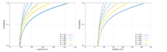
The cumulative probability distributions (7), as functions of the magnetic rigidity for various zenith angles, are displayed in Figure 4. There, lower magnetic rigidities are associated with particle trajectories having small zenith angles. Notice that both plots are qualitatively different and this probably is evidence of the complexity of the GF present at the two very distinct latitudes.
4.2 Primary Flux Corrected by GF
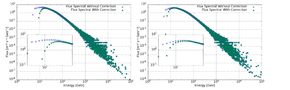
As was explained in section 3.1.2, once the penumbral CDFs is obtained, it is possible to refine the calculation of the expected primary flux and the corresponding flux of background secondaries at ground level. In Figure 5 the GCR flux and are displayed for both LAGO sites: BGA and BRC. Only those primaries producing secondaries at ground level are shown. In both cases, the influence of the GF corrections is only significant at lower energies, GeV. As expected, instead of a sharp cutoff as in the standard case, a smooth cutoff is observed, corresponding to the different rigidities cutoff in the different regimes, and the flux of primaries is affected according with figure 4, i.e., a bigger effect for BGA (rigidity up to GV) than BRC (rigidity up to GV).
The primary flux interacts with the atmosphere and produces the secondary flux at the ground level. These interactions were simulated by CORSIKA obtaining a very comprehensive distribution of particles at the detector level. To estimate the response of the WCD to each type of secondary particle, this flux is analyzed using a detailed Geant4 simulation of the LAGO detector will be described and the first preliminary results were showed by Otiniano et al. (2015).
4.3 Secondary Flux Corrected by GF
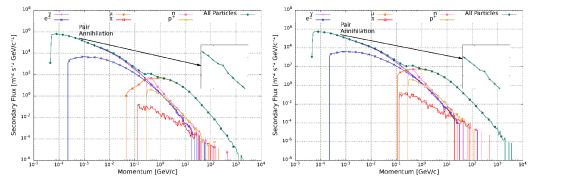
Figure 6 displays the simulated spectra of secondaries (under secular conditions) at both cities. A noticeable peak for the distribution of secondary neutrons and protons are evident at both sites. At these low altitudes, a muon hump is also visible in the distribution spectra, and this is typically used as a calibration point for WCD (see e.g. Etchegoyen et al., 2005; H. Asorey for the LAGO Collaboration, 2013).
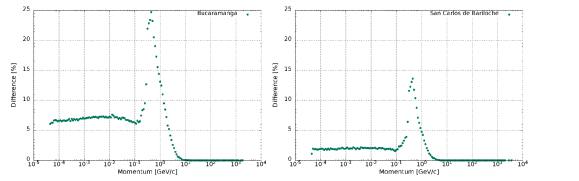
By defining the flux percentage difference, , it is possible to get a better understanding of the energy range where the geomagnetic corrections are more important, specially when dynamic variations are considered. Thus
| (16) |
where are the indices corresponding to the configuration of the GF introduced in the section 3.1.2. To evaluate the impact of this new method, the differences between cases (standard calculation) and (new method), as a function of the secondary particles momentum, are illustrated in Figure 7. The presence of a peak at MeV/c is evident for both sites in the distribution, located between MeV/c and GeV/c. For lower energies, the difference is a bit larger at BGA than at BRC, as we expected after figure 3. When we explored in more detail the particle component of the secondaries at these momenta, we found that these differences are dominated by secondary neutrons (Suárez-Durán, 2015), where the diminution is of the order of . This result, in our simulation, agree with the fact that variations in the flux registered by Neutron Monitors are a proxy of the changing conditions in the near-earth space environment. For energies higher than GeV, corrections are not important.
Finally, this tool allows the study of the impact of dynamic conditions of the GF in the distribution of secondary particles by comparing secular conditions of the GF with the evolution of the GF states as a function of time, . This is because the calculations performed by this method are focusing on the background of the GCR flux, e.g., we did not consider the solar particle event during the geomagnetic storm of May 13-17, 2005, but just the influence of the state of the GF, for this UTC-time, over the background of GCR flux. This is shown in Figure 8, where the time evolution of is displayed at both sites for May of 2005. We have selected this particular month because the strong geomagnetic storm on May 13-17, 2005, generated intense disturbances in the GF (see e.g. Adekoya et al., 2012; Bisi et al., 2010; Galav et al., ). Three particular cases are shown: the total flux secondary particles, , the muon flux and the neutron flux . It is clear that, beside the time coincidence of the flux variations, it is more significant at Bucaramanga than at Bariloche, and that the neutron flux at ground level is the most affected component by the GF activity, which reinforces the known sensitivity of this particular constituent for the observation of geomagnetic disturbances (see e.g. Belov et al., 2005).
As reference, on the background of each sub-plot in figure 8 (gray line) the flux of neutrons at ground level is shown, registered by two Neutron Monitors (NM) with similar rigidities to both sites; i.e. of GV for NM of ESOI and GV for NM of Mexico. As reference, the for BGA is GV and for BRC is GV. Both NM show a decrease between and in elapsed UTC time, that is in coincidence with our simulation results. Because we have simulated the effect of the GF under GCR flux, i.e., we do not simulate solar particle events, it is possible, with our approach, to estimate the contribution of the GF topology to a Forbush decrease event.

5 Final remarks
In this paper, we have presented the LAGO space weather chain of simulations devised to obtain precise calculations of secondary particle flux at ground level that can be used at every geographical position. It takes into account geomagnetic corrections for both secular (long term phenomena with typical time scale larger than a year) and transient events (with typical time scales of hours to days). We shall consider all calculations performed without this new method as a first approximation to the more precise determination of the real flux of secondaries particles, calculated when the effects of the geomagnetic field are fully considered.
Variations of the flux of secondaries at two LAGO sites with different latitude/longitude (Bucaramanga, N, W and San Carlos de Bariloche N, W) were calculated for both secular geomagnetic conditions and under transient events, during the geomagnetic active month of May 2005. Our simulations show that the secondary flux is sensitive to the latitude and that the secondary neutrons at the ground level are the most affected flux component due to variations of the geomagnetic field during space weather phenomena. While our calculation relies on the isotropy of the GCR flux, it is important to note that during certain FDs, small anisotropies in the flux of primaries could be induced by the configuration of the incoming magnetic cloud and the disturbances of the geomagnetic field during these particular events. Actually a anisotropy in the flux of secondary muons was observed at ground level during the Forubush decrease of December 13, 2006 (Kane, 2006; Fushishita et al., 2010). However, since our WCD are not sensitive to the arrival direction of secondary particles, we will not be able to detect such small effect while the total flux of secondaries remains constant.
Several dedicated clusters and a Grid-based implementation have been deployed for these calculations. A dedicated Virtual Organization, lagoproject, part of the European Grid Infrastructure (EGI, http://www.egi.eu) activities has been created, and available tools for Grid have been adapted and implemented to run CORSIKA in a absolutely transparent way to the user.
The standard definition of the penumbra region for magnetic rigidities generates a complex structure of particle trajectories: permitted, prohibited and quasi-trapped orbits, which does not allow to derive all values for the (Smart et al., 2006). Currently, calculations of rigidity cutoff tend not to consider the effects involved in the penumbra, and always use a single effective value (equation (3)) to account and characterize all the complexity of involved effects (Smart and Shea, 2009). In this paper the concept of rigidity cutoff has been generalized as a time dependent function of the cumulative probability distribution (see equation (10)). With this refinement, at the penumbra region, we can obtain a non-vanishing probability to have an incoming particle (with a zenithal angle ) contributing to the flux of primaries at the observation point.
Combining the data measured at different locations of the LAGO detection network, with those obtained from the detailed simulation performed by this space weather chain, we are now capable of providing a better understanding of the temporal evolution and of the small and large scales disturbances of the space weather phenomena.
Acknowledgements.
The authors thanks the enlightening suggestions and criticism from the anonymous referees and also from the AGU Space Weather Editorial Office which have helped to make this work clearer and more focused. We appreciate the support of Vicerrectoría Investigación y Extensión Universidad Industrial de Santander for its permanent sponsorship, and acknowledge the financial support of Departamento Administrativo de Ciencia, Tecnología e Innovación of Colombia (COLCIENCIAS) under contracts FP44842-051-2015 and FP44842-661-2015. The authors acknowledge the support of COLCIENCIAS, CONICET and MINCyT for funding bilateral cooperation Argentina-Colombia, grant AR:CO-15/02 CO:729-2015. HA and MSD acknowledge the support from Innóvate Perú, grant 398-PNICP-PIBA-2014. Significant parts of the calculations needed for this work was performed with the computational support of the Centros de Supercomputación y Cálculo Científico de la Universidad Industrial de Santander. We also acknowledge the NMDB database (www.nmdb.eu), founded under the European Union’s FP7 programme (contract no. 213007) for providing the data. Neutron monitor of the Emilio Segre Observatory is supported by collaboration ICRC-ESO (Tel Aviv University and Israel Space Agency, Israel) and University “Roma Tre” with IFSI-CNR (Italy). Neutron monitor data of Mexico City is provided by the Cosmic Ray Group of the Geophysical Institute at the Universidad Autónoma de México (UNAM). The authors are grateful to the LAGO and Pierre Auger Observatory Collaboration members (http://lagoproject.org/collab.html) for their continuous engagement and support.References
- A. Galindo for the LAGO Collaboration (2015) A. Galindo for the LAGO Collaboration (2015), Sensitivity of LAGO and Calibration of a Water-Cherenkov Detector in Sierra Negra, México. , in ICRC 2015 Id. ICRC2015_673, vol. ICRC2015.
- Abbasi et al. (2008) Abbasi, R., M. Ackermann, J. Adams, M. Ahlers, J. Ahrens, K. Andeen, J. Auffenberg, X. Bai, M. Baker, B. Baret, S. W. Barwick, R. Bay, J. L. Bazo Alba, K. Beattie, T. Becka, J. K. Becker, K. H. Becker, P. Berghaus, D. Berley, E. Bernardini, D. Bertrand, D. Z. Besson, J. W. Bieber, E. Blaufuss, D. J. Boersma, C. Bohm, J. Bolmont, S. Böser, O. Botner, J. Braun, D. Breder, T. Burgess, T. Castermans, D. Chirkin, B. Christy, J. Clem, D. F. Cowen, M. V. D’Agostino, M. Danninger, A. Davour, C. T. Day, C. De Clercq, L. Demirörs, O. Depaepe, F. Descamps, P. Desiati, G. de Vries-Uiterweerd, T. DeYoung, J. C. Diaz-Velez, J. Dreyer, J. P. Dumm, M. R. Duvoort, W. R. Edwards, R. Ehrlich, J. Eisch, R. W. Ellsworth, O. Engdegaard, S. Euler, P. A. Evenson, O. Fadiran, A. R. Fazely, K. Filimonov, C. Finley, M. M. Foerster, B. D. Fox, A. Franckowiak, R. Franke, T. K. Gaisser, J. Gallagher, R. Ganugapati, L. Gerhardt, L. Gladstone, A. Goldschmidt, J. A. Goodman, R. Gozzini, D. Grant, T. Griesel, A. Gross, S. Grullon, R. M. Gunasingha, M. Gurtner, C. Ha, A. Hallgren, F. Halzen, K. Han, K. Hanson, D. Hardtke, R. Hardtke, Y. Hasegawa, J. Heise, K. Helbing, M. Hellwig, P. Herquet, S. Hickford, G. C. Hill, K. D. Hoffman, K. Hoshina, D. Hubert, J. P. Hülss, P. O. Hulth, K. Hultqvist, S. Hundertmark, R. L. Imlay, M. Inaba, A. Ishihara, J. Jacobsen, G. S. Japaridze, H. Johansson, J. M. Joseph, K. H. Kampert, A. Kappes, T. Karg, A. Karle, H. Kawai, J. L. Kelley, J. Kiryluk, F. Kislat, S. R. Klein, S. Klepser, G. Kohnen, H. Kolanoski, L. Köpke, M. Kowalski, T. Kowarik, M. Krasberg, K. Kuehn, T. Kuwabara, M. Labare, K. Laihem, H. Landsman, R. Lauer, H. Leich, D. Leier, A. Lucke, J. Lundberg, J. Lünemann, J. Madsen, R. Maruyama, K. Mase, H. S. Matis, C. P. McParland, K. Meagher, A. Meli, M. Merck, T. Messarius, P. Mészáros, H. Miyamoto, A. Mohr, T. Montaruli, R. Morse, S. M. Movit, K. Münich, R. Nahnhauer, J. W. Nam, P. Niessen, D. R. Nygren, S. Odrowski, A. Olivas, M. Olivo, M. Ono, S. Panknin, S. Patton, C. Pérez de los Heros, J. Petrovic, A. Piegsa, D. Pieloth, A. C. Pohl, R. Porrata, N. Potthoff, J. Pretz, P. B. Price, G. T. Przybylski, R. Pyle, K. Rawlins, S. Razzaque, P. Redl, E. Resconi, W. Rhode, M. Ribordy, A. Rizzo, W. J. Robbins, J. Rodrigues, P. Roth, F. Rothmaier, C. Rott, C. Roucelle, D. Rutledge, D. Ryckbosch, H. G. Sander, S. Sarkar, K. Satalecka, S. Schlenstedt, T. Schmidt, D. Schneider, O. Schultz, D. Seckel, B. Semburg, S. H. Seo, Y. Sestayo, S. Seunarine, A. Silvestri, A. J. Smith, C. Song, G. M. Spiczak, C. Spiering, T. Stanev, T. Stezelberger, R. G. Stokstad, M. C. Stoufer, S. Stoyanov, E. A. Strahler, T. Straszheim, K. H. Sulanke, G. W. Sullivan, Q. Swillens, I. Taboada, O. Tarasova, A. Tepe, S. Ter-Antonyan, S. Tilav, M. Tluczykont, P. A. Toale, D. Tosi, D. Turcan, N. van Eijndhoven, J. Vandenbroucke, A. Van Overloop, V. Viscomi, C. Vogt, B. Voigt, C. Walck, T. Waldenmaier, H. Waldmann, M. Walter, C. Wendt, S. Westerhoff, N. Whitehorn, C. H. Wiebusch, C. Wiedemann, G. Wikström, D. R. Williams, R. Wischnewski, H. Wissing, K. Woschnagg, X. W. Xu, G. Yodh, and S. Yoshida (2008), Solar Energetic Particle Spectrum on 2006 December 13 Determined by IceTop, The Astrophysical Journal, 689(1), L65–L68, 10. 1086/595679.
- Abraham et al. (2007) Abraham, J., P. Abreu, M. Aglietta, C. Aguirre, D. Allard, I. Allekotte, J. Allen, P. Allison, C. Alvarez, J. Alvarez-Muniz, M. Ambrosio, L. Anchordoqui, S. Andringa, A. Anzalone, C. Aramo, S. Argiro, K. Arisaka, E. Armengaud, F. Arneodo, F. Arqueros, T. Asch, H. Asorey, P. Assis, B. S. Atulugama, J. Aublin, M. Ave, G. Avila, T. Backer, D. Badagnani, A. F. Barbosa, D. Barnhill, S. L. C. Barroso, P. Bauleo, J. Beatty, T. Beau, B. R. Becker, K. H. Becker, J. A. Bellido, S. BenZvi, C. Berat, T. Bergmann, P. Bernardini, X. Bertou, P. L. Biermann, P. Billoir, O. Blanch-Bigas, F. Blanco, P. Blasi, C. Bleve, H. Blumer, M. Bohacova, C. Bonifazi, R. Bonino, M. Boratav, J. Brack, P. Brogueira, W. C. Brown, P. Buchholz, A. Bueno, N. G. Busca, K. S. Caballero-Mora, B. Cai, D. V. Camin, R. Caruso, W. Carvalho, A. Castellina, O. Catalano, G. Cataldi, L. Cazon-Boado, R. Cester, J. Chauvin, A. Chiavassa, J. A. Chinellato, A. Chou, J. Chye, P. D. J. Clark, R. W. Clay, E. Colombo, R. Conceicao, B. Connolly, F. Contreras, J. Coppens, A. Cordier, U. Cotti, S. Coutu, C. E. Covault, A. Creusot, J. Cronin, S. Dagoret-Campagne, K. Daumiller, B. R. Dawson, R. M. de Almeida, C. De Donato, S. J. de Jong, G. De La Vega, W. J. M. de Mello Junior, J. R. T. de Mello Neto, I. De Mitri, V. de Souza, L. del Peral, O. Deligny, A. D. Selva, C. D. Fratte, H. Dembinski, C. Di Giulio, J. C. Diaz, C. Dobrigkeit, J. C. D’Olivo, D. Dornic, A. Dorofeev, J. C. dos Anjos, M. T. Dova, D. D’Urso, M. A. DuVernois, R. Engel, L. Epele, M. Erdmann, C. O. Escobar, A. Etchegoyen, P. F. S. Luis, H. Falcke, G. Farrar, A. C. Fauth, N. Fazzini, A. Fernandez, F. Ferrer, S. Ferry, B. Fick, A. Filevich, A. Filipcic, I. Fleck, R. Fonte, C. E. Fracchiolla, W. Fulgione, B. Garcia, D. Garcia Gamez, D. Garcia-Pinto, X. Garrido, H. Geenen, G. Gelmini, H. Gemmeke, P. L. Ghia, M. Giller, H. Glass, M. S. Gold, G. Golup, F. G. Albarracin, M. G. Berisso, R. G. Herrero, P. Goncalves, M. G. do Amaral, D. Gonzalez, J. G. Gonzalez, M. Gonzalez, D. Gora, A. Gorgi, P. Gouffon, V. Grassi, A. Grillo, C. Grunfeld, Y. Guardincerri, F. Guarino, G. P. Guedes, J. Gutierrez, J. D. Hague, J. C. Hamilton, P. Hansen, D. Harari, S. Harmsma, J. L. Harton, A. Haungs, T. Hauschildt, M. D. Healy, T. Hebbeker, D. Heck, C. Hojvat, V. C. Holmes, P. Homola, J. Horandel, A. Horneffer, M. Horvat, M. Hrabovsky, T. Huege, M. Iarlori, A. Insolia, F. Ionita, A. Italiano, M. Kaducak, K. H. Kampert, B. Keilhauer, E. Kemp, R. M. Kieckhafer, H. O. Klages, M. Kleifges, J. Kleinfeller, R. Knapik, J. Knapp, D. H. Koang, A. Kopmann, A. Krieger, O. Kromer, D. Kumpel, N. Kunka, A. Kusenko, G. La Rosa, C. Lachaud, B. L. Lago, D. Lebrun, P. LeBrun, J. Lee, M. A. L. de Oliveira, A. Letessier-Selvon, M. Leuthold, I. Lhenry-Yvon, R. Lopez, A. Lopez Aguera, J. L. Bahilo, M. C. Maccarone, C. Macolino, S. Maldera, M. Malek, G. Mancarella, M. E. Mancenido, D. Mandat, P. Mantsch, A. G. Mariazzi, I. C. Maris, D. Martello, J. Martínez, O. M. Bravo, H. J. Mathes, J. Matthews, J. a. J. Matthews, G. Matthiae, D. Maurizio, P. O. Mazur, T. McCauley, M. McEwen, R. R. McNeil, M. C. Medina, G. Medina-Tanco, A. Meli, D. Melo, E. Menichetti, A. Menschikov, C. Meurer, R. Meyhandan, M. I. Micheletti, G. Miele, W. Miller, S. Mollerach, M. Monasor, D. M. Ragaigne, F. Montanet, B. Morales, C. Morello, E. Moreno, J. C. Moreno, C. Morris, M. Mostafa, M. A. Muller, R. Mussa, G. Navarra, J. L. Navarro, S. Navas, L. Nellen, C. Newman-Holmes, D. Newton, T. N. Thi, N. Nierstenhofer, D. Nitz, D. Nosek, L. Nozka, J. Oehlschlager, T. Ohnuki, A. Olinto, V. M. Olmos-Gilbaja, M. Ortiz, S. Ostapchenko, L. Otero, D. P. Selmi-Dei, M. Palatka, J. Pallotta, G. Parente, E. Parizot, S. Parlati, S. Pastor, M. Patel, T. Paul, V. Pavlidou, K. Payet, M. Pech, J. Pekala, R. Pelayo, I. M. Pepe, L. Perrone, S. Petrera, P. Petrinca, Y. Petrov, D. Ngoc, D. Ngoc, T. N. P. Thi, A. Pichel, R. Piegaia, T. Pierog, M. Pimenta, T. Pinto, V. Pirronello, O. Pisanti, M. Platino, J. Pochon, T. A. Porter, P. Privitera, M. Prouza, E. J. Quel, J. Rautenberg, S. Reucroft, B. Revenu, F. a. S. Rezende, J. Ridky, S. Riggi, M. Risse, C. Riviere, V. Rizi, M. Roberts, C. Robledo, G. Rodriguez, D. R. Frias, J. R. Martino, J. R. Rojo, I. Rodriguez-Cabo, G. Ros, J. Rosado, M. Roth, B. Rouille-d’Orfeuil, E. Roulet, A. C. Rovero, F. Salamida, H. Salazar, G. Salina, F. Sanchez, M. Santander, C. E. Santo, E. M. Santos, F. Sarazin, S. Sarkar, R. Sato, V. Scherini, H. Schieler, F. Schmidt, T. Schmidt, O. Scholten, P. Schovanek, F. Schussler, S. J. Sciutto, M. Scuderi, A. Segreto, D. Semikoz, M. Settimo, R. C. Shellard, I. Sidelnik, B. B. Siffert, G. Sigl, N. S. De Grande, A. Smialkowski, R. Smida, A. G. K. Smith, B. E. Smith, G. R. Snow, P. Sokolsky, P. Sommers, J. Sorokin, H. Spinka, R. Squartini, E. Strazzeri, A. Stutz, F. Suarez, T. Suomijarvi, A. D. Supanitsky, M. S. Sutherland, J. Swain, Z. Szadkowski, J. Takahashi, A. Tamashiro, A. Tamburro, O. Tascau, R. Tcaciuc, D. Thomas, R. Ticona, J. Tiffenberg, C. Timmermans, W. Tkaczyk, C. J. T. Peixoto, B. Tome, A. Tonachini, D. Torresi, P. Travnicek, A. Tripathi, G. Tristram, D. Tscherniakhovski, M. Tueros, V. Tunnicliffe, R. Ulrich, M. Unger, M. Urban, J. F. V. Galicia, I. Valino, L. Valore, A. M. van den Berg, V. van Elewyck, R. A. Vazquez, D. Veberic, A. Veiga, A. Velarde, T. Venters, V. Verzi, M. Videla, L. Villasenor, S. Vorobiov, L. Voyvodic, H. Wahlberg, O. Wainberg, T. Waldenmaier, P. Walker, D. Warner, A. A. Watson, S. Westerhoff, G. Wieczorek, L. Wiencke, B. Wilczynska, H. Wilczynski, C. Wileman, M. G. Winnick, H. Wu, B. Wundheiler, J. Xu, T. Yamamoto, P. Younk, E. Zas, D. Zavrtanik, M. Zavrtanik, A. Zech, A. Zepeda, and M. Ziolkowski (2007), Correlation of the Highest-Energy Cosmic Rays with Nearby Extragalactic Objects, Science, 318(5852), 938–943, 10. 1126/science. 1151124.
- Adekoya et al. (2012) Adekoya, B. J., V. U. Chukwuma, N. O. Bakare, and T. W. David (2012), On the effects of geomagnetic storms and pre storm phenomena on low and middle latitude ionospheric F2, Astrophysics and Space Science, 340(2), 217–235, 10. 1007/s10509-012-1082-x.
- Agostinelli et al. (2003) Agostinelli, S., J. Allison, K. Amako, J. Apostolakis, H. Araujo, P. Arce, M. Asai, D. Axen, S. Banerjee, G. Barrand, F. Behner, L. Bellagamba, J. Boudreau, L. Broglia, A. Brunengo, H. Burkhardt, S. Chauvie, J. Chuma, R. Chytracek, G. Cooperman, G. Cosmo, P. Degtyarenko, A. Dell’Acqua, G. Depaola, D. Dietrich, R. Enami, A. Feliciello, C. Ferguson, H. Fesefeldt, G. Folger, F. Foppiano, A. Forti, S. Garelli, S. Giani, R. Giannitrapani, D. Gibin, J. J. Gómez-Cádenas, I. González, G. G. Abril, G. Greeniaus, W. Greiner, V. Grichine, A. Grossheim, S. Guatelli, P. Gumplinger, R. Hamatsu, K. Hashimoto, H. Hasui, A. Heikkinen, A. Howard, V. Ivanchenko, A. Johnson, F. W. Jones, J. Kallenbach, N. Kanaya, M. Kawabata, Y. Kawabata, M. Kawaguti, S. Kelner, P. Kent, A. Kimura, T. Kodama, R. Kokoulin, M. Kossov, H. Kurashige, E. Lamanna, T. Lampén, V. Lara, V. Lefebure, F. Lei, M. Liendl, W. Lockman, F. Longo, S. Magni, M. Maire, E. Medernach, K. Minamimoto, P. M. de Freitas, Y. Morita, K. Murakami, M. Nagamatu, R. Nartallo, P. Nieminen, T. Nishimura, K. Ohtsubo, M. Okamura, S. O’Neale, Y. Oohata, K. Paech, J. Perl, A. Pfeiffer, M. G. Pia, F. Ranjard, A. Rybin, S. Sadilov, E. D. Salvo, G. Santin, T. Sasaki, N. Savvas, Y. Sawada, S. Scherer, S. Sei, V. Sirotenko, D. Smith, N. Starkov, H. Stoecker, J. Sulkimo, M. Takahata, S. Tanaka, E. Tcherniaev, E. S. Tehrani, M. Tropeano, P. Truscott, H. Uno, L. Urban, P. Urban, M. Verderi, A. Walkden, W. Wander, H. Weber, J. P. Wellisch, T. Wenaus, D. C. Williams, D. Wright, T. Yamada, H. Yoshida, and D. Zschiesche (2003), Geant4 - a simulation toolkit, Nuclear Instruments and Methods in Physics Research Section A: Accelerators, Spectrometers, Detectors and Associated Equipment, 506(3), 250–303, 10. 1016/S0168-9002(03)01368-8.
- Allard et al. (2008) Allard, D., I. Allekotte, C. Alvarez, H. Asorey, H. Barros, X. Bertou, O. Burgoa, M. G. Berisso, O. Martínez, P. M. Loza, T. Murrieta, G. Perez, H. Rivera, A. Rovero, O. Saavedra, H. Salazar, J. C. Tello, R. T. Peralda, A. Velarde, and L. Villaseñor (2008), Use of water-cherenkov detectors to detect gamma ray bursts at the large aperture GRB observatory (lago), Nuclear Instruments and Methods in Physics Research Section A: Accelerators, Spectrometers, Detectors and Associated Equipment, 595(1), 70 – 72, http://dx. doi. org/10. 1016/j. nima. 2008. 07. 041, RICH 2007Proceedings of the Sixth International Workshop on Ring Imaging Cherenkov Detectors.
- Asorey et al. (2015) Asorey, H., S. Dasso, and the LAGO Collaboration (2015), LAGO: the latin american giant observatory, in The 34th International Cosmic Ray Conference, vol. PoS(ICRC2015), p. 247.
- Asorey et al. (2016) Asorey, H., R. Mayo-García, L. A. Núñez, M. Rodríguez-Pascual, A. J. Rubio-Montero, M. Suarez-Durán, L. A. Torres-Niño, and LAGO Collaboration (2016), The latin american giant observatory: a successful collaboration in latin america based on cosmic rays and computer science domains, in Proceedings of the 16th IEEE/ACM International Symposium on Cluster, Cloud, and Grid Computing, pp. 707–711, IEEE.
- Asorey et al. (2017) Asorey, H., L. A. Núñez, C. Y. Pérez Arias, S. Pinilla, F. Quinonez, and M. Suárez-Durán (2017), Astroparticle Techniques: Simulating cosmic rays induced background radiation on aircrafts, in Revista Mexicana de Astronomia y Astrofisica Conference Series, Revista Mexicana de Astronomia y Astrofisica, vol. 27, vol. 49, pp. 57–57.
- Asorey, H. for The Pierre Auger Collaboration (2011) Asorey, H. for The Pierre Auger Collaboration (2011), Measurement of Low Energy Cosmic Radiation with the Water Cherenkov Detector Array of the Pierre Auger Observatory, in Proceedings of the 33th ICRC, pp. 41–44, Beijing, China.
- Barbera et al. (2011) Barbera, R., M. Fargetta, and R. Rotondo (2011), A simplified access to grid resources by science gateways, in Proceedings of The International Symposium on Grids and Clouds, vol. PoS(ISGC 2011 & OGF 31), p. 23, Taipei, Taiwan.
- Belov et al. (2005) Belov, A., L. Baisultanova, E. Eroshenko, H. Mavromichalaki, V. Yanke, V. Pchelkin, C. Plainaki, and G. Mariatos (2005), Magnetospheric effects in cosmic rays during the unique magnetic storm on November 2003, Journal of Geophysical Research: Space Physics, 110(A9), 1–9, 10. 1029/2005JA011067.
- Belov et al. (2014) Belov, A., A. Abunin, M. Abunina, E. Eroshenko, V. Oleneva, V. Yanke, A. Papaioannou, H. Mavromichalaki, N. Gopalswamy, and S. Yashiro (2014), Coronal mass ejections and non-recurrent forbush decreases, Solar Physics, 289(10), 3949–3960, 10. 1007/s11207-014-0534-6.
- Bisi et al. (2010) Bisi, M. M., A. R. Breen, B. V. Jackson, R. A. Fallows, A. P. Walsh, Z. Mikić, P. Riley, C. J. Owen, A. Gonzalez-Esparza, E. Aguilar-Rodriguez, H. Morgan, E. A. Jensen, A. G. Wood, M. J. Owens, M. Tokumaru, P. K. Manoharan, I. V. Chashei, A. S. Giunta, J. A. Linker, V. I. Shishov, S. A. Tyul’bashev, G. Agalya, S. K. Glubokova, M. S. Hamilton, K. Fujiki, P. P. Hick, J. M. Clover, and B. Pintér (2010), From the sun to the earth: The 13 may 2005 coronal mass ejection, Solar Physics, 265(1), 49–127, 10.1007/s11207-010-9602-8.
- Calderón et al. (2015) Calderón, R., H. Asorey, and L. A. Núñez (2015), Geant4 based simulation of the water cherenkov detectors of the lago project, Nuclear and Particle Physics Proceedings, pp. 424–426.
- Cane (2000) Cane, H. (2000), Coronal Mass Ejections and Forbush Decreases, Space Science Reviews, 93(1-2), 55–77, 10. 1023/A:1026532125747.
- Carmichael et al. (1969) Carmichael, H., M. A. Shea, D. F. Smart, and J. R. McCall (1969), Iv. geographically smoothed geomagnetic cutoffs, Canadian Journal of Physics, 47(19), 2067–2072, 10. 1139/p69-260.
- Cooke et al. (1991) Cooke, D. J., J. E. Humble, M. A. Shea, D. F. Smart, N. Lund, I. L. Rasmussen, B. Byrnak, P. Goret, and N. Petrou (1991), On cosmic-ray cut-off terminology, Il Nuovo Cimento C, 14(3), 213–234, 10. 1007/BF02509357.
- Dasso et al. (2012) Dasso, S., H. Asorey, and Pierre Auger Collaboration (2012), The scaler mode in the pierre auger observatory to study heliospheric modulation of cosmic rays, Advances in Space Research, 49, 1563–1569, 10. 1016/j. asr. 2011. 12. 028.
- Dasso et al. (2015) Dasso, S., A. M. Gulisano, J. J. Masías-Meza, H. Asorey, and the LAGO Collaboration (2015), A project to install water-cherenkov detectors in the antarctic peninsula as part of the LAGO detection network, in The 34th International Cosmic Ray Conference, vol. PoS(ICRC2015), p. 105.
- Desorgher (2004) Desorgher, L. (2004), The magnetocosmics code, Tech. rep., Technical report, http://cosray. unibe. ch/~ laurent/magnetoscosmics.
- Dorman et al. (2008) Dorman, L. I., O. A. Danilova, N. Iucci, M. Parisi, N. G. Ptitsyna, M. I. Tyasto, and G. Villoresi (2008), Effective non-vertical and apparent cutoff rigidities for a cosmic ray latitude survey from antarctica to italy in minimum of solar activity, Advances in Space Research, 42(3), 510 – 516, http://dx. doi. org/10. 1016/j. asr. 2007. 04. 032.
- Etchegoyen et al. (2005) Etchegoyen, A., P. Bauleo, X. Bertou, C. B. Bonifazi, A. Filevich, M. C. Medina, D. G. Melo, A. C. Rovero, A. D. Supanitsky, and A. Tamashiro (2005), Muon-track studies in a water cherenkov detector, Nuclear Instruments and Methods in Physics Research Section A: Accelerators, Spectrometers, Detectors and Associated Equipment, 545(3), 602 – 612, http://dx. doi. org/10. 1016/j. nima. 2005. 02. 016.
- Forbush (1937) Forbush, S. E. (1937), On the effects in the cosmic-ray intensity observed during recent magnetic storm, Physical Review, 51, 1108–1109.
- Fushishita et al. (2010) Fushishita, A., T. Kuwabara, C. Kato, S. Yasue, J. W. Bieber, P. Evenson, M. R. D. Silva, A. D. Lago, N. J. Schuch, M. Tokumaru, M. L. Duldig, J. E. Humble, I. Sabbah, H. K. A. Jassar, M. M. Sharma, and K. Munakata (2010), Precursors of the forbush decrease on 2006 decembre 14 observed with the global muon detector network (gmdn), The Astrophysical Journal, 715(2), 1239–1247, 10.1088/0004-637X/715/2/1239.
- (26) Galav, P., S. S. Rao, S. Sharma, G. Gordiyenko, and R. Pandey (), Ionospheric response to the geomagnetic storm of 15 may 2005 over midlatitudes in the day and night sectors simultaneously, Journal of Geophysical Research: Space Physics, 119(6), 5020–5031, 10.1002/2013JA019679.
- H. Asorey and S. Dasso and L. A. Núñez and Y. Pérez and C. Sarmiento-Cano and M. Suárez-Durán for the LAGO Collaboration (2015) H. Asorey and S. Dasso and L. A. Núñez and Y. Pérez and C. Sarmiento-Cano and M. Suárez-Durán for the LAGO Collaboration (2015), The LAGO space weather program: Directional geomagnetic effects, background fluence calculations and multi-spectral data analysis, in The 34th International Cosmic Ray Conference, vol. PoS(ICRC2015), p. 142.
- H. Asorey for the LAGO Collaboration (2013) H. Asorey for the LAGO Collaboration (2013), The LAGO Solar Project, in Proceedings of the 33th International Cosmic Ray Conference ICRC 2013, pp. 1–4, Rio de Janeiro, Brasil.
- Heck et al. (1998) Heck, D., J. Knapp, J. N. Capdevielle, G. Schatz, and T. Thouw (1998), CORSIKA: a Monte Carlo code to simulate extensive air showers. .
- Hess and Demmelmair (1937) Hess, V. F., and A. Demmelmair (1937), World-wide effect in cosmic ray intensity, as observed during a recent magnetic storm, Nature, 140, doi:10. 1038/140316a0.
- Huedo et al. (2001) Huedo, E., R. S. Montero, and I. M. Llorente (2001), The gridway framework for adaptive scheduling and execution on grids, Scalable Computing: Practice and Experience, 6(3).
- I. Sidelnik for the LAGO Collaboration (2015) I. Sidelnik for the LAGO Collaboration (2015), The sites of the latin american giant observatory, in The 34th International Cosmic Ray Conference, vol. PoS(ICRC2015), p. 665.
- International Association of Geomagnetism and Aeronomy, Working Group V-MOD (2010) International Association of Geomagnetism and Aeronomy, Working Group V-MOD (2010), International Geomagnetic Reference Field: the eleventh generation, Geophysical Journal International, 183(3), 1216–1230, 10. 1111/j. 1365-246X. 2010. 04804. x.
- Kane (2006) Kane, R. P. (2006), Cosmic ray anisotropies around the forbush decrease of april 11, 2001, Solar Physics, 234(2), 353–362, 10.1007/s11207-006-0083-8.
- Kneizys et al. (1996) Kneizys, F. X., L. W. Abreu, G. P. Anderson, J. H. Chetwynd, et al. (1996), The MODTRAN 2/3 report and LOWTRAN 7 model, Tech. rep.
- Letessier-Selvon and Stanev (2011) Letessier-Selvon, A., and T. Stanev (2011), Ultrahigh energy cosmic rays, Rev. Mod. Phys., 83, 907–942, 10. 1103/RevModPhys. 83. 907.
- Lockwood (1971) Lockwood, J. A. (1971), Forbush decreases in the cosmic radiation, Space Science Reviews, 12(5), 658–715, 10. 1007/BF00173346.
- Masías-Meza and Dasso (2014) Masías-Meza, J. J., and S. Dasso (2014), Geomagnetic effects on cosmic ray propagation under different conditions for buenos aires and marambio, argentina, Sun and Geosphere, 9, 41–47.
- NOAA (1976) NOAA (1976), U. S. STANDARD ATMOSPHERE (1976), Tech. rep., NASA.
- NOAA (2009) NOAA (2009), The Global Data Assimilation System (GDAS).
- Ostapchenko (2011) Ostapchenko, S. (2011), Monte Carlo treatment of hadronic interactions in enhanced Pomeron scheme: QGSJET-II model, Physical Review D, 83(1), 014,018, 10. 1103/PhysRevD. 83. 014018.
- Otiniano et al. (2015) Otiniano, L., F. Quispe, and the LAGO Collaboration (2015), Development of a High Altitude LAGO Site in Peru, in ICRC 2015 Id. ICRC2015_688, vol. ICRC2015.
- Pinilla et al. (2015) Pinilla, S. A., H. Asorey, and L. A. Nuñez (2015), Cosmic Rays Induced Background Radiation on Board of Commercial Flights, in Nuclear and Particle Physics Proceedings, vol. 267-269, pp. 418–420, 10. 1016/j. nuclphysbps. 2015. 10. 139.
- Rodriguez-Pascual et al. (2013) Rodriguez-Pascual, M., R. Mayo-García, and I. M. Llorente (2013), Montera: a framework for efficient execution of monte carlo codes on grid infrastructures, Computing and Informatics, 32(1), 113–144.
- Rodriguez-Pascual et al. (2015) Rodriguez-Pascual, M., G. LaRocca, C. . Kanellopoulo, C. Carrubba, G. . Inserra, R. Ricceri, H. Asorey, A. J. Rubio-Montero, E. Núñez-González, L. A. Núñez, O. Prnjat, R. Barbera, and R. Mayo-García (2015), A resilient methodology for accessing and exploiting data and scientific codes on distributed environments, in Computational Science and Engineering (CSE), 2015 IEEE 18th International Conference on, pp. 319–323, IEEE.
- Rubio-Montero et al. (2015a) Rubio-Montero, A. J., E. Huedo, F. Castejón, and R. Mayo-García (2015a), Gwpilot: Enabling multi-level scheduling in distributed infrastructures with gridway and pilot jobs, Future Generation Computer Systems, 45, 25–52.
- Rubio-Montero et al. (2015b) Rubio-Montero, A. J., E. Huedo, and R. Mayo-García (2015b), User-guided provisioning in federated clouds for distributed calculations, in International Workshop on Adaptive Resource Management and Scheduling for Cloud Computing, pp. 60–77, Springer.
- Schrijver et al. (2015) Schrijver, C. J., K. Kauristie, A. D. Aylward, C. M. Denardini, S. E. Gibson, A. Glover, N. Gopalswamy, M. Grande, M. Hapgood, D. Heynderickx, N. Jakowski, V. V. Kalegaev, G. Lapenta, J. a. Linker, S. Liu, C. H. Mandrini, I. R. Mann, T. Nagatsuma, D. Nandi, T. Obara, T. P. O’Brien, T. Onsager, H. J. Opgenoorth, M. Terkildsen, C. E. Valladares, and N. Vilmer (2015), Understanding space weather to shield society: A global road map for 2015-2025 commissioned by COSPAR and ILWS, Advances in Space Research, (4), 63.
- Shea et al. (1965) Shea, M. A., D. F. Smart, and K. G. McCracken (1965), A study of vertical cutoff rigidities using sixth degree simulations of the geomagnetic field, Journal of Geophysical Research, 70(17), 4117–4130, 10. 1029/JZ070i017p04117.
- Simpson et al. (1953) Simpson, J. A., W. Fonger, and S. B. Treiman (1953), Cosmic radiation intensity-time variations and their origin. i. neutron intensity variation method and meteorological factors, Physical Review, 90(5), 934.
- Singer (1954) Singer, S. F. (1954), Lectures on the primary cosmic radiation, Il Nuovo Cimento (1943-1954), 11, 369–376.
- Smart and Shea (2009) Smart, D. F., and M. A. Shea (2009), Fifty years of progress in geomagnetic cutoff rigidity determinations, Advances in Space Research, 44(10), 1107–1123.
- Smart and Shea (2012) Smart, D. F., and M. A. Shea (2012), VERTICAL GEOMAGNETIC CUTOFF RIGIDITIES FOR EPOCH 2000 — DEVIATIONS FROM EXPECTED LATITUDE CURVES, pp. 277–285, World Scientific Publishing Company, 10. 1142/9789812707185_0022.
- Smart et al. (2006) Smart, D. F., M. A. Shea, A. J. Tylka, and P. R. Boberg (2006), A geomagnetic cutoff rigidity interpolation tool: Accuracy verification and application to space weather, Advances in Space Research, 37(6), 1206–1217.
- Suárez-Durán (2015) Suárez-Durán, M. (2015), Modulación de rayos cósmicos a nivel del suelo por cambios en el campo geomagnético, para la colaboración lago, Master thesis, Escuela de Física, Universidad Industrial de Santander, Bucaramanga, Colombia.
- The Pierre Auger Collaboration (2011) The Pierre Auger Collaboration (2011), The Pierre Auger Observatory scaler mode for the study of solar activity modulation of galactic cosmic rays, Journal of Instrumentation, 6(01), P01,003–P01,003, 10. 1088/1748-0221/6/01/P01003.
- The Pierre Auger Collaboration (2015) The Pierre Auger Collaboration (2015), The pierre auger cosmic ray observatory, Nuclear Instruments and Methods in Physics Research Section A: Accelerators, Spectrometers, Detectors and Associated Equipment, 798, 172 – 213, http://dx. doi. org/10. 1016/j. nima. 2015. 06. 058.
- Tsyganenko (2002) Tsyganenko, N. A. (2002), A model of the near magnetosphere with a dawn-dusk asymmetry 1. Mathematical structure, Journal of Geophysical Research: Space Physics, 107(A8), SMP 12–1–SMP 12–15, 10. 1029/2001JA000219.
- Usoskin et al. (2008) Usoskin, I. G., I. Braun, O. G. Gladysheva, J. R. Hörandel, T. Jämsén, G. A. Kovaltsov, and S. A. Starodubtsev (2008), Forbush Decreases of Cosmic Rays: Energy Dependence of The Recovery Phase, Journal of Geophysical Research: Space Physics, 113(A7), 10. 1029/2007JA012955.
- Vargas et al. (2015) Vargas, S., C. Mantilla, O. Martínez, N. Vázquez, D. Cazar-Ramírez, and the LAGO Collaboration (2015), Lago ecuador, implementing a set of wcd detectors for space weather research: first results and further developments, in The 34th International Cosmic Ray Conference, vol. PoS(ICRC2015), p. 135.
- Weigel et al. (2009) Weigel, R. S., D. N. Baker, D. A. Roberts, and T. King (2009), Using virtual observatories for heliophysics research, Eos, Transactions American Geophysical Union, 90(47), 441–442, 10. 1029/2009EO470001.
- Wiebel-Sooth et al. (1998) Wiebel-Sooth, B., P. L. Biermann, and H. Meyer (1998), Vii. individual element spectra: prediction and data, Astronomy and Astrophysics, 330, 389–398.