Magnetic properties of Type I and II Weyl Semi-metals in Superconducting state.

Abstract

Superconductivity was observed in certain range of pressure and chemical composition in Weyl semi-metals of both the type I and type II (when the Dirac cone tilt parameter $\kappa>1$). Magnetic properties of these superconductors are studied on the basis of microscopic phonon mediated pairing model. The Ginzburg - Landau effective theory for the order parameter is derived using Gorkov approach and used to determine anisotropic coherence length, the penetration depth determining the Abrikosov parameter for a layered material and applied to recent extensive experiments on $MoTe_{2}$. It is found that superconductivity is of second kind near the topological transition at $\kappa=1$. For a larger tilt parameter superconductivity becomes first kind. For $\kappa<1$ the Abrikosov parameter also tends to be reduced, often crossing over to the first kind. For the superconductors of the second kind the dependence of critical fields $H_{c2}$ and $H_{c1}$ on the tilt parameter $\kappa$ (governed by pressure) is compared with the experiments. Strength of thermal fluctuations is estimated and its is found that they are strong enough to cause Abrikosov vortex lattice melting near $H_{c2}$. The melting line is calculated and is consistent with experiments provided the fluctuations are three dimensional in the type I phase (large pressure) and two dimensional in the type II phase (small pressure).

I Introduction

Dispersion relation near Fermi surface in recently synthesized two and three dimensional Weyl (Dirac) semi-metalsWeng ; MoTeearly ; ZrTe is qualitatively distinct from conventional metals, semi - metals or semiconductors, in which all the bands are parabolic. In type I Weyl semi-metals (WSM), the band inversion results in Weyl points in low-energy excitations being anisotropic massless ”relativistic” fermions. They exhibit several remarkable properties like the chiral magnetic effectchiral related to the chiral anomaly in particle physics. More recently, type-II WSMs, layered transition-metal dichalcogenides, were discoveredSoluyanov . Here, the Weyl cone exhibits such a strong tilt, so that they can be characterized by a nearly flat band at Fermi surface. The type-II WSM also exhibit exotic properties different from the type-I ones, such anti-chiral effect of the chiral Landau level,Yu and novel quantum oscillations Brien .

Graphene is a prime example of the type I WSM, while materials, like layered organic compound $\alpha-(BEDT-TTF)_{2}I_{3}$, were long suspectedGoerbig1 to be a 2D type-II Dirac fermion. Several materials were observed to undergo the I to II transition while doping or pressure is changedtoptransition . Theoretically physics of the topological (Lifshitz) phase transitions between the type I to type II Weyl semi-metals were considered in the context of superfluid phaseVolovik A of $He_{3}$, layered organic materials in 2DGoerbig2 and 3D Weyl semi-metalsYe . The pressure modifies the spin orbit coupling that in turn determines the topology of the Fermi surface of these novel materials Sun .

Many Weyl materials are known to be superconducting. A detailed study of superconductivity in WSM under hydrostatic pressure revealed a curious dependence of critical temperature of the superconducting transition on pressure. The critical temperature $T_{c\text{ }}$ in some of these systems like $HfTe_{5}$ showHfTe a sharp maximum as a function of pressure. This contrasts with generally smooth dependence on pressure in other superconductors (not suspected to be Weyl materials) like a high $T_{c}$ cuprateYBCO $YBCO$. Since superconductivity is especially affected by the type I to II topological transition, it might serve as such an indicatorZyuzin ; Rosenstein17 .

Various mechanisms of superconductivity in WSM turned superconductors have been considered theoretically DasSarma ; FuBerg ; frontiers , however evidence point towards the conventional phonon mediated one. If the Fermi level is not situated too close to the Dirac point, the BCS type pairing occurs, otherwise a more delicate formalism should be employedShapiro14 . A theory predicted possibility of superconductivity in the type II Weyl semimetals was developed recently in the framework of Eliashberg model Zyuzin ; Rosenstein17 .

In the present paper we extend the study of superconductivity in Weyl semimetals of both types to magnetic properties and thermal fluctuations. The phenomenological Ginzburg-Landau theory for superconducting WSM of the arbitrary type is microscopically derived and used to establish magnetic phase diagram. In particular the Abrikosov parameter used to distinguish between the superconductivity of the first from the second kind is determined. It turns out that superconductivity is of second kind near the critical value of the tilt parameter $\kappa=1$, marking the topological transition, but becomes first kind away from it on both the type I and type II sides. The critical fields, coherence lengths magnetic penetration depths and the Ginzburg number characterizing the strength of fluctuations are found. In the strongly layered material likeTamai $MoTe_{2}$ the fluctuations are strong enough to qualitatively affect the Abrikosov vortex phase diagram: the lattice ”melts” into the vortex liquid MoTe2melting . This is reminiscent of a well known (possibly non - Weyl semi-metal) layered dichalcogenides superconductor $NbSe_{2}$ that is perhaps the only low $T_{c}$ material with fluctuations strong enough to exhibit vortex lattice meltingNbSe2 . The Ginzburg number for these single crystals is of order of $Gi=10^{-4}$ with similar $T_{c}$ and upper critical field $H_{c2}\left(0\right)$ of several $Tesla$.

The focus generally is on the dependence of the properties in the cone tilt parameter $\kappa$ and consequently on the transition from Type-I to type-II WSM variations. This is experimentally measured in experiments on the pressure (determining $\kappa$) dependence of WSM superconductors. These days there are already quite a variety of WSM turned superconductors and it is impossible to model all of them in a single paper. Therefore one of the best studied material, $MoTe_{2}$ is chosen as a representative example. A major reason is that magnetic properties of this superconductor were investigated in a wide range pressuresMoTe2melting from ambient to $30GPa$ (controlling the tilt parameter $\kappa$ of the WSM, see below). An additional advantage of this choice is that the strongly layered material $MoTe_{2}$ in many aspects behaves as a simpler two dimensional WSM (weak van der Waals coupling between the layers is easily accounted for).

The paper is organized as follows. The next section contains the formulation of a sufficiently general the phonon mediated BCS - like model of anisotropic type I and II WSM. Gor’kov equations are written with details relegated to appendices. The section III is devoted to derivation from the Gor’kov equations in the inhomogeneous case of the coefficients of the Ginzburg - Landau equations including the gradient term. Magnetic properties are derived from the GL model in section IV, while thermal fluctuations are subject of section V. In particular vortex lattice melting line is considered. Section VI contains conclusions and discussion of the experimental data on $MoTe_{2}$.

II Pairing in Weyl semimetal.

II.1 The model

Considering layered WSM as alternating superconducting 2D layers separated by dielectric streaks. We assume that a 3D electrons with strongly anisotropic dispersion relation are paired inside the 2D layers only. We start to study the effect of the topological transition on superconductivity using the simplest possible model of a single 2D WSM layer with just two sublattices denoted by $\alpha=1,2$ and expand this model to real 3D layered system. The band structure near the Fermi level of a 2D Weyl semi-metal is well captured by the non-interacting massless Weyl Hamiltonian with the Fermi velocity $v$ (assumed to be isotropic in the $x-y$ plane) and conventional parabolic term on $z-$direction Rosenstein17 :

$$K = \int_{\mathbf{r}}\psi_{\alpha}^{s+}\left(\mathbf{r}\right)\widehat{K}_{\alpha\beta}\psi_{\beta}^{s}\left(\mathbf{r}\right)\text{\ \ \ \ }$$ (1)

$$\text{\ \ }\widehat{K}_{\gamma\delta} = -i\hbar v\nabla^{i}\sigma_{\gamma\delta}^{i}+\left(-i\hbar w_{i}\nabla^{i}-\mu+\frac{p_{z}^{2}}{2m_{z}}\right)\delta_{\gamma\delta}\text{.}$$

Here $\mu$ is the chemical potential, $p_{z}=-i\hbar\nabla_{z}$ , $\sigma$ are Pauli matrices in the sublattice space and $s$ is spin projection. The velocity vector $\mathbf{w}$ defines the tilt of the (otherwise isotropic) cone. (We use below the dimensionless ratio $\kappa=w/v$ as tilt parameter describing cone axis projection in $x$ direction). The graphene - like dispersion relation for $\mathbf{w}=0$ represents the type I Weyl semi-metal, while for the velocity $\left|\mathbf{w}\right|=w$ exceeding $v$, the material becomes a type II Weyl semi - metal.

Generally there are a number of pairs of points (Weyl cones) constituting the Fermi ”surface” of such a material at chemical potential $\mu=0$. We restrict ourself to the case of just one left handed and one right handed Dirac points, typically but not always separated in the Brillouin zone. Generalization to include the opposite chirality and several ”cones” is straightforward. We assume that different valleys are paired independently and drop the valley indices (multiplying the density of states by $2N_{f}$).

The effective electron-electron attraction due to the electron - phonon attraction opposed by Coulomb repulsion (pseudopotential) mechanism creates pairing below $T_{c}$. Further we assume the singlet $s$-channel interaction with essentially local interaction,

$$V=\frac{g^{2}}{2}\ \int d\mathbf{r}\text{ }\psi_{\alpha}^{+\uparrow}\left(\mathbf{r}\right)\psi_{\beta}^{\downarrow+}\left(\mathbf{r}\right)\psi_{\beta}^{\uparrow}\left(\mathbf{r}\right)\psi_{\alpha}^{\downarrow}\left(\mathbf{r}\right)\text{,}$$ (2)

where the coupling $g^{2}$ is zero between the layers. As usual the retarded interaction has a cutoff frequency $\Omega$, so that it is active in an energy shell of width $2\hbar\Omega$ around the Fermi level Abrikosov . For the phonon mechanism it is the Debye frequency. We first remindRosenstein17 , the Gorkov equations and then derive from them the phenomenological GL equations that allow to obtain the basic magnetic response of the superconductors.

II.2 Green Functions and Gor’kov equations

Finite temperature properties of the condensate are described at temperature $T$ by the normal and the anomalous Matsubara Greens functionsAbrikosov (GF),

$$G_{\alpha\beta}^{ts}\left(\mathbf{r}\tau,\mathbf{r}^{\prime}\tau^{\prime}\right) = -\left\langle T_{\tau}\psi_{\alpha}^{t}\left(\mathbf{r}\tau\right)\psi_{\beta}^{s+}\left(\mathbf{r}^{\prime}\tau^{\prime}\right)\right\rangle=\delta^{ts}g_{\alpha\beta}\left(\mathbf{r-r}^{\prime},\tau-\tau^{\prime}\right);$$ (3)

$$F_{\alpha\beta}^{ts}\left(\mathbf{r}\tau,\mathbf{r}^{\prime}\tau^{\prime}\right) = \left\langle T_{\tau}\psi_{\alpha}^{t}\left(\mathbf{r}\tau\right)\psi_{\beta}^{s}\left(\mathbf{r}^{\prime}\tau^{\prime}\right)\right\rangle=-\varepsilon^{ts}f_{\alpha\beta}\left(\mathbf{r-r}^{\prime},\tau-\tau^{\prime}\right);$$

$$F_{\alpha\beta}^{+ts}\left(\mathbf{r}\tau,\mathbf{r}^{\prime}\tau^{\prime}\right) = \left\langle T_{\tau}\psi_{\alpha}^{t+}\left(\mathbf{r}\tau\right)\psi_{\beta}^{s+}\left(\mathbf{r}^{\prime}\tau^{\prime}\right)\right\rangle=\varepsilon^{ts}f_{\alpha\beta}^{+}\left(\mathbf{r-r}^{\prime},\tau-\tau^{\prime}\right).$$

where $t,s$ are the spin indexes. The set of Gor’kov equations in the time translation invariant, yet inhomogeneous case isRosenstein17 ; Rosenstein18 ,

$$L_{\gamma\beta}^{1}g_{\beta\kappa}\left(\mathbf{r,r}^{\prime}\ \omega\right) = \delta^{\gamma\kappa}\delta\left(\mathbf{r-r}^{\prime}\right)-\Delta_{\alpha\gamma}\left(\mathbf{r,}\tau=0\right)f_{\alpha\kappa}^{+}\left(\mathbf{r,r}^{\prime},\omega\right);$$ (4)

$$L_{\gamma\beta}^{2}f_{\beta\kappa}^{+}\left(\mathbf{r,r}^{\prime},\omega\right) = \Delta_{\beta\gamma}^{\ast}\left(\mathbf{r,}\tau=0\right)g_{\beta\kappa}\left(\mathbf{r,r}^{\prime},\omega\right)\text{.}$$

Here the two Weyl operators are, (tilt vector $\mathbf{w}$ is assumed to be directed along $x$- axes)

$$L_{\gamma\beta}^{1} = \left[\left(i\omega+\mu^{\prime}+iw\nabla_{x}\right)\delta_{\gamma\beta}-iv\sigma_{\gamma\beta}^{i}\ \nabla_{r}^{i}\right];$$ (5)

$$L_{\gamma\beta}^{2} = \left[\left(-i\omega+\mu^{\prime}+iw\nabla_{x}\right)\delta_{\gamma\beta}-iv\sigma_{\gamma\beta}^{it}\nabla_{r}^{i}\right]\text{,}$$

Here $\mu^{\prime}=\mu-\frac{p_{z}^{2}}{2m_{z}}.$

The gap function defined as

$$\Delta_{\beta\kappa}^{\ast}\left(\mathbf{r}\right)=g^{2}T\sum\limits_{\omega}f_{\beta\kappa}^{+}\left(\mathbf{r,}\omega\right).$$ (6)

The gap function in the s-wave channel is $\Delta_{\alpha\gamma}\left(\mathbf{r}\right)=\sigma_{\alpha\gamma}^{x}\Delta\left(\mathbf{r}\right).$ This is the starting point for derivation of the GL free energy functional of $\Delta\left(\mathbf{r}\right)$.

III Derivation of GL equations (without magnetic field)

In this section the Ginzburg - Landau equations in a homogeneous material (including the gradient terms) is derived. Magnetic field and fluctuations effects will be discussed in the next two section by generalizing the basic formalism.

III.1 The integral form the Gorkov equations

To derive the GL equations including the derivative term one needs the integral form of the Gor’kov equations (see Appendix A), Eq.(4):

$$g_{\epsilon\kappa}\left(\mathbf{r,r}^{\prime},\omega\right) = \mathrm{g}_{\epsilon\kappa}^{1}\left(\mathbf{r}-\mathbf{r}^{\prime},\omega\right)-\int_{\mathbf{r}^{\prime\prime}}\mathrm{g}_{\epsilon\theta}^{1}\left(\mathbf{r}-\mathbf{r}^{\prime\prime},\omega\right)\Delta_{\theta\phi}^{\ast}\left(\mathbf{r}^{\prime\prime}\right)f_{\phi\kappa}^{+}\left(\mathbf{r}^{\prime\prime}\mathbf{,r}^{\prime},\omega\right);$$ (7)

$$f_{\beta\kappa}^{+}\left(\mathbf{r,r}^{\prime},\omega\right) = \int_{\mathbf{r}^{\prime\prime\prime}}\mathrm{g}_{\beta\alpha}^{2}\left(\mathbf{r-r}^{\prime\prime\prime},-\omega\right)\Delta_{\alpha\epsilon}^{\ast}\left(\mathbf{r}^{\prime\prime\prime}\right)\times$$

$$\left\{\mathrm{g}_{\epsilon\kappa}^{1}\left(\mathbf{r}^{\prime\prime\prime}-\mathbf{r}^{\prime},\omega\right)-\int_{\mathbf{r}^{\prime\prime}}\mathrm{g}_{\epsilon\theta}^{1}\left(\mathbf{r}^{\prime\prime}-\mathbf{r}^{\prime\prime\prime},\omega\right)\Delta_{\theta\phi}^{\ast}\left(\mathbf{r}^{\prime\prime}\right)f_{\phi\kappa}^{+}\left(\mathbf{r}^{\prime\prime}\mathbf{,r}^{\prime},\omega\right)\right\}\text{.}$$

Here $\mathrm{g}_{\beta\kappa}^{1}\left(\mathbf{r,r}^{\prime}\right)$ and $\mathrm{g}_{\beta\kappa}^{2}\left(\mathbf{r,r}^{\prime}\right)$ are GF of operators $L_{\gamma\beta}^{1}$ and $L_{\gamma\beta}^{2}$ :

$$L_{\gamma\beta}^{1}\mathrm{g}_{\beta\kappa}^{1}\left(\mathbf{r,r}^{\prime}\right)=\delta^{\gamma\kappa}\delta\left(\mathbf{r-r}^{\prime}\right);L_{\gamma\beta}^{2}\mathrm{g}_{\beta\kappa}^{2}\left(\mathbf{r,r}^{\prime}\right)=\delta^{\gamma\kappa}\delta\left(\mathbf{r-r}^{\prime}\right).$$ (8)

This will be enough do derive the GL expansion to the third order in the gap function $\Delta\left(\mathbf{r}\right)$ that will be used as an order parameterAbrikosov .

III.2 The GL expansion

Using the first and the second iteration of equations Eq.(7) and specializing on the case $\mathbf{r}=\mathbf{r}^{\prime}$, one rewrites the Gorkov’s equation Eq.(4) as (see details in Appendix A):

$$\Delta\left(\mathbf{r}\right)=\frac{g^{2}T}{2}\sum\limits_{\omega}\left\{K\left(\mathbf{r-r}_{1}\right)\Delta\left(\mathbf{r}_{1}\right)-Q\left(\mathbf{r,r}_{1},\mathbf{r}_{2},\mathbf{r}_{3}\right)\Delta\left(\mathbf{r}_{2}\right)\Delta\left(\mathbf{r}_{3}\right)\Delta\left(\mathbf{r}_{1}\right)\right\}\text{.}$$ (9)

Here integrations over variables $\mathbf{r}_{1}$, $\mathbf{r}_{2}$, $\mathbf{r}_{3}$ are implied. Kernel of the linear in $\Delta$ term is

$$K\left(\mathbf{r}\right)=\mathrm{g}_{21}^{2}\left(\mathbf{r}\right)\mathrm{g}_{21}^{1}\left(-\mathbf{r}\right)+\mathrm{g}_{11}^{2}\left(\mathbf{r}\right)\mathrm{g}_{22}^{1}\left(-\mathbf{r}\right)+\mathrm{g}_{12}^{2}\left(\mathbf{r}\right)\mathrm{g}_{12}^{1}\left(-\mathbf{r}\right)+\mathrm{g}_{22}^{2}\left(\mathbf{r}\right)\mathrm{g}_{11}^{1}\left(-\mathbf{r}\right)\text{,}$$ (10)

while the coefficient of the cubic term is,

$$Q=\begin{array}[]{c}\mathrm{g}_{21}^{2}\left(\mathbf{r-r}_{3}\right)\mathrm{g}_{21}^{1}\left(\mathbf{r}_{2}\mathbf{-r}_{3}\right)\mathrm{g}_{21}^{2}\left(\mathbf{r}_{2}\mathbf{-r}_{1}\right)\mathrm{g}_{21}^{1}\left(\mathbf{r}_{1}\mathbf{-r}\right)+\\ \ \mathrm{g}_{21}^{2}\left(\mathbf{r-r}_{3}\right)\mathrm{g}_{22}^{1}\left(\mathbf{r}_{2}\mathbf{-r}_{3}\right)\mathrm{g}_{11}^{2}\left(\mathbf{r}_{2}\mathbf{-r}_{1}\right)\mathrm{g}_{21}^{1}\left(\mathbf{r}_{1}\mathbf{-r}\right)+\\ \ \mathrm{g}_{22}^{2}\left(\mathbf{r-r}_{3}\right)\mathrm{g}_{11}^{1}\left(\mathbf{r}_{2}\mathbf{-r}_{3}\right)\mathrm{g}_{22}^{2}\left(\mathbf{r}_{2}\mathbf{-r}_{1}\right)\mathrm{g}_{11}^{1}\left(\mathbf{r}_{1}\mathbf{-r}\right)+\\ \mathrm{g}_{22}^{2}\left(\mathbf{r-r}_{3}\right)\mathrm{g}_{12}^{1}\left(\mathbf{r}_{2}\mathbf{-r}_{3}\right)\mathrm{g}_{12}^{2}\left(\mathbf{r}_{2}\mathbf{-r}_{1}\right)\mathrm{g}_{11}^{1}\left(\mathbf{r}_{1}\mathbf{-r}\right)+\\ \mathrm{g}_{11}^{2}\left(\mathbf{r-r}_{3}\right)\mathrm{g}_{21}^{1}\left(\mathbf{r}_{2}\mathbf{-r}_{3}\right)\mathrm{g}_{21}^{2}\left(\mathbf{r}_{2}\mathbf{-r}_{1}\right)\mathrm{g}_{22}^{1}\left(\mathbf{r}_{1}\mathbf{-r}\right)+\\ \mathrm{g}_{11}^{2}\left(\mathbf{r-r}_{3}\right)\mathrm{g}_{22}^{1}\left(\mathbf{r}_{2}\mathbf{-r}_{3}\right)\mathrm{g}_{11}^{2}\left(\mathbf{r}_{2}\mathbf{-r}_{1}\right)\mathrm{g}_{22}^{1}\left(\mathbf{r}_{1}\mathbf{-r}\right)+\\ \mathrm{g}_{12}^{2}\left(\mathbf{r-r}_{3}\right)\mathrm{g}_{11}^{1}\left(\mathbf{r}_{2}\mathbf{-r}_{3}\right)\mathrm{g}_{22}^{2}\left(\mathbf{r}_{2}\mathbf{-r}_{1}\right)\mathrm{g}_{12}^{1}\left(\mathbf{r}_{1}\mathbf{-r}\right)+\\ \mathrm{g}_{12}^{2}\left(\mathbf{r-r}_{3}\right)\mathrm{g}_{12}^{1}\left(\mathbf{r}_{2}\mathbf{-r}_{3}\right)\mathrm{g}_{12}^{2}\left(\mathbf{r}_{2}\mathbf{-r}_{1}\right)\mathrm{g}_{12}^{1}\left(\mathbf{r}_{1}\mathbf{-r}\right)\text{.}\end{array}$$ (11)

Using the Fourier transformation for the GF,

$$\mathrm{g}_{\alpha\beta}^{2,1}\left(\mathbf{r}\right)=\sum\nolimits_{\mathbf{p}}g_{\alpha\beta}^{2,1}\left(\mathbf{p}\right)e^{i\mathbf{p\cdot r}},\Delta\left(\mathbf{r}\right)=\sum\nolimits_{\mathbf{q}}\Delta\left(\mathbf{q}\right)e^{i\mathbf{q\cdot r}}$$ (12)

,

and substituting them into Eqs. (10) and (11), one obtains, after expansion in momenta, the first GL equation,

$$\Delta\left(\mathbf{r}\right)=\frac{g^{2}T}{2}\sum\limits_{\omega,\mathbf{p}}\ \left\{a\left(\mathbf{p}\right)\Delta\left(\mathbf{r}\right)\mathbf{+}C_{ki}\left(\mathbf{p}\right)\frac{\partial^{2}\Delta\left(\mathbf{r}\right)}{\partial\mathbf{r}_{i}\partial\mathbf{r}_{k}}-b\left(\mathbf{p}\right)\Delta^{3}\left(\mathbf{r}\right)\right\}\text{.}$$ (13)

The function appearing in an expression for the coefficient $a$ is:

$$a\left(\mathbf{p}\right)=g_{21}^{2}\left(\mathbf{p}\right)g_{21}^{1}\left(\mathbf{p}\right)+g_{11}^{2}\left(\mathbf{p}\right)g_{22}^{1}\left(\mathbf{p}\right)+g_{12}^{2}\left(\mathbf{p}\right)g_{12}^{1}\left(\mathbf{p}\right)+g_{22}^{2}\left(\mathbf{p}\right)g_{11}^{1}\left(\mathbf{p}\right)\text{,}$$ (14)

while the gradient term coefficients take a form:

$$C_{ki}\left(\mathbf{p}\right)=\frac{1}{2}\left\{\begin{array}[]{c}\frac{\partial g_{21}^{2}\left(\mathbf{p}\right)}{\partial p_{k}}\frac{\partial g_{21}^{1}\left(\mathbf{p}\right)}{\partial p_{i}}+\frac{\partial g_{11}^{2}\left(\mathbf{p}\right)}{\partial p_{k}}\frac{\partial g_{22}^{1}\left(\mathbf{p}\right)}{\partial p_{i}}+\\ \frac{\partial g_{12}^{2}\left(\mathbf{p}\right)}{\partial p_{k}}\frac{\partial g_{12}^{1}\left(\mathbf{p}\right)}{\partial p_{i}}+\frac{\partial g_{22}^{2}\left(\mathbf{p}\right)}{\partial p_{k}}\frac{\partial g_{11}^{1}\left(\mathbf{p}\right)}{\partial p_{i}}\end{array}\right\}\text{.}$$ (15)

The cubic term’s coefficient is given by

$$b\left(\mathbf{p}\right)=\left\{\begin{array}[]{c}g_{21}^{2}\left(\mathbf{p}\right)g_{22}^{1}\left(-\mathbf{p}\right)g_{11}^{2}\left(-\mathbf{p}\right)g_{21}^{1}\left(\mathbf{p}\right)+g_{21}^{2}\left(\mathbf{p}\right)g_{21}^{1}\left(-\mathbf{p}\right)g_{21}^{2}\left(-\mathbf{p}\right)g_{21}^{1}\left(\mathbf{p}\right)+\\ g_{22}^{2}\left(\mathbf{p}\right)g_{11}^{1}\left(-\mathbf{p}\right)g_{22}^{2}\left(-\mathbf{p}\right)g_{11}^{1}\left(\mathbf{p}\right)+g_{22}^{2}\left(\mathbf{p}\right)g_{12}^{1}\left(-\mathbf{p}\right)g_{12}^{2}\left(-\mathbf{p}\right)g_{11}^{1}\left(\mathbf{p}\right)+\\ g_{11}^{2}\left(\mathbf{p}\right)g_{21}^{1}\left(-\mathbf{p}\right)g_{21}^{2}\left(-\mathbf{p}\right)g_{22}^{1}\left(\mathbf{p}\right)+g_{11}^{2}\left(\mathbf{p}\right)g_{22}^{1}\left(-\mathbf{p}\right)g_{11}^{2}\left(-\mathbf{p}\right)g_{22}^{1}\left(\mathbf{p}\right)\ +\\ g_{12}^{2}\left(\mathbf{p}\right)g_{11}^{1}\left(-\mathbf{p}\right)g_{22}^{2}\left(-\mathbf{p}\right)g_{12}^{1}\left(\mathbf{p}\right)+g_{12}^{2}\left(\mathbf{p}\right)g_{12}^{1}\left(-\mathbf{p}\right)g_{12}^{2}\left(-\mathbf{p}\right)g_{12}^{1}\left(\mathbf{p}\right)\end{array}\right\}\text{.}$$ (16)

The integrations are carried out in the following subsection.

III.3 Calculation of the coefficients of the GL expansion in a WSM layer.

III.3.1 Linear homogeneous term

There are two linear in $\Delta$ terms in Eq.(13). In momentum space the sum is:

$$a\left(T\right)=\frac{T}{2}\sum\limits_{\omega,\mathbf{p}}\ a\left(\mathbf{p}\right)-\frac{1}{g^{2}}.$$ (17)

Substituting the normal GF, calculated in Appendix B for 2D (meaning $p_{z}$ terms in propagators are ignored) is, into Eqs.(8,5)

, one obtains coefficient of the linear term,

$$a\left(\mathbf{p}\right)=2Z^{-1/2}\left\{\left(vp\right)^{2}+\omega^{2}+\left(\mu-w_{x}p_{x}\right)^{2}\right\}\text{,}$$ (18)

where

$$\sqrt{Z}=\left(\omega^{2}+\left(\mu-w_{x}p_{x}-vp\right)^{2}\right)\left(\omega^{2}+\left(\mu-w_{x}p_{x}+vp\right)^{2}\right)\text{.}$$ (19)

Here and later in the section $\mathbf{p=}\left\{p_{x},p_{y}\right\}$.

Performing summation on Matsubara frequencies and integration over the 2D momentum (within the adiabatic approximation, $\mu>>\Omega$, see details in Appendix C and in Rosenstein17 ) in Eq.(17), one obtains:

$$a\left(T\right)=f\ln\frac{T_{c}}{T}\approx\ f\left(1-\frac{T}{T_{c}}\right).$$ (20)

The critical temperature has the expression (see details in Rosenstein17 ) (see Fig.1)

$$T_{c}=1.14\Omega\exp\left[-1/\lambda\right],$$ (21)

with the effective electron-electron strength in the WSM given by

$$\lambda=\lambda_{0}f,\lambda_{0}=\mu g^{2}/2\pi v^{2}\hbar^{2}\text{.}$$

The quantity $f$ as a function of the cone tilt parameter $\kappa=w/v$ is different on the two sides of the topological phase transition of the WSMRosenstein17 . For the type I WSM, $\kappa<1$, in which the Fermi surface is a closed ellipsoid, it is given by:

$$f=\frac{1}{\left(1-\kappa^{2}\right)^{3/2}}\text{.}$$ (22)

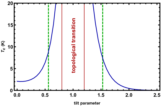
Figure 1: Critical temperature as a function of the tilt parameter $\kappa$ indicates Type-I and Type II phases of WSM (Green dashed lines marks $T_{c}$ for two topological phases of $MoTe_{2}$). Red lines mark the range where the BCS approximation is not valid.

In the type II phase, $\kappa>1$, the Fermi surface becomes open, extending over the Brillouin zone, and the corresponding expression is:

$$f=\frac{\kappa^{2}}{\ \pi\left(\kappa^{2}-1\right)^{3/2}}\left\{2\sqrt{1+\kappa}-1+\log\left[\frac{2\left(\kappa^{2}-1\right)}{\kappa\left(1+\sqrt{1+\kappa}\right)^{2}\delta}\right]\right\}\text{.}$$ (23)

Here $\delta$ is an ultraviolet cut off parameter $\delta=a\Omega/w\pi$, where $a$ is an interatomic spacing. These expression appear in all the physical quantities calculated below expressing the topological phase transition. Let us now turn to the gradient terms.

III.3.2 The gradient terms

Components $C_{xy}$ and $C_{yx}$ of the second derivative tensor $C$ are zero due to the reflection symmetry in $p_{y}$ direction , when the cone tilt vector $\mathbf{w}$ is directed along the $x$ axis (see Appendix D for details). After integration over momenta in the second term in equation Eq.(13), the gradient terms coefficients are,

$$C_{xx}=\frac{v^{2}\hslash^{2}}{T_{c}^{2}}\eta_{x},\text{ \ }C_{yy}=\frac{v^{2}\hslash^{2}}{T_{c}^{2}}\eta_{y}\text{,}$$ (24)

where dimensionless integrals $\eta_{x}$ and $\eta_{y}$ are given in Eqs.(73,85) of Appendix D.

III.3.3 Cubic term

The coefficient of a term cubic in $\Delta$ in the GL equation Eq.(13) reads:

$$b\left(\mathbf{p}\right)=2Z^{-1}\left\{\left(vp\right)^{2}\ +\omega^{2}+\left(\mu-w_{x}p_{x}\right)^{2}\right\}\left\{\left(vp\right)^{2}\ +\omega^{2}+\left(\mu+w_{x}p_{x}\right)^{2}\right\}\text{.}$$ (25)

After integration over momentum, the GL coefficient is obtained

$$\beta=\frac{\eta}{\mu T_{c}},$$ (26)

with $\eta$ given in Appendix D, Eq.(87). Having determined the coefficients of the GL equations, we now turn to discussion of the coherence lengths and the resulting in - plane anisotropy due to the tilt of the Dirac cone.

III.4 In plane coherence lengths and anisotropy

III.4.1 Coherence lengths

The first GL equation in WSM in magnetic field (required in the following section) is standard:

$$-\left(\xi_{x}^{2}\partial_{x}^{2}+\xi_{y}^{2}\partial_{y}^{2}\right)\Delta\left(\mathbf{r}\right)-\tau\Delta\left(\mathbf{r}\right)+\frac{\beta}{f}\left|\Delta\left(\mathbf{r}\right)\right|^{2}\Delta\left(\mathbf{r}\right)=0\text{.}$$ (27)

Here $\tau=1-T/T_{c}$. Comparing coefficients of linear terms in Eq.(27), the coherence lengths are

$$\xi_{x}^{2}=C_{xx}/f,\xi_{y}^{2}=C_{yy}/f\text{,}$$ (28)

and are computed numerically.

To be specific the in plane correlations lengths are calculated for a $MoTe_{2}$ single crystals that were extensively studied experimentally at pressures between ambient to $30GPa$. The coherence lengths $\xi_{x}$ and $\xi_{y}$ as functions of the tilt ration $\kappa=w/v$ for material parameters pertinent to $MoTe_{2}$ are shown in Fig. 1 as solid blue and green lines respectively. We estimate the Debye frequency from the Raman dataMoTe2melting , $\Omega=100K$. Fermi velocity $v=5\cdot 10^{7}cm/s$ and Fermi energy, $\mu=8\Omega$, from ARPESMoTeearly . An ultraviolet cutoff for Eq.(23) is taken to be an interatomic distance $a=0.3nm$ ($T_{c}$ depends logarithmically on it, see Eq.(23). The electron - electron coupling due to phonons $\lambda_{0}=g^{2}\mu/2\pi v^{2}\hbar^{2}$ is assumed to be linearly dependent of $\kappa$ (or pressure that presumably determines $\kappa$): $\lambda_{0}=\lambda_{0}^{I}-\alpha\kappa$ for $\lambda_{0}^{I}=0.25$ and $\alpha=0.05$.

One observes that the both coherence lengths are large and roughly equal at small $\kappa$. Below $\kappa=0.2$ the curve flattens reaching value of $\xi_{x}=\xi_{y}=45nm$ for graphene - like material at $\kappa=0$. In the topological transition region (marked in Fig.2a by red lines) they become very small. In the type II phase the two coherence length are different and become large again.  In the critical region the theory becomes inapplicable.

III.4.2 In plane anisotropy

The anisotropy parameter is defined as $\varepsilon=\xi_{x}/\xi_{y}=\sqrt{C_{xx}/C_{yy}}$. It is plotted as a function of $\kappa$ in Fig.2b. The coherence length in $z-$direction $\xi_{z}$ as a function of tilt parameter $\kappa$ is presented in Fig.2c.

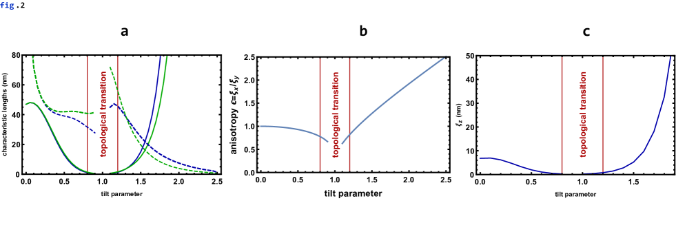
Figure 2: a. Dependence of characteristic lengths of the Weyl superconductor on the tilt parameter $\kappa$. The topological (Lifshitz) transition occurs at $\kappa\rightarrow 1$. Coherence lengths along the $x$ (blue) and $y$ (green) directions are solid lines. Same for the penetration depth times $\sqrt{2}$ as dashed lines. b. In-plane anisotropy of the coherence length $\xi_{x}/\xi_{y}$ (same as the ratio of penetration depths $\lambda_{y}/\lambda_{x}$)  as function of the tilt parameter. c. Characteristic length $\xi_{z}$ in direction perpendicular to the layers on the tilt parameter $\kappa$. Here the thickness of single layer $s=3nm,$ and interlayer distance $d=10nm.$

Graphene - like superconductor is isotropic. At small $\kappa$ the anisotropy is small with $\epsilon<1$. Above the topological phase transition line it increases rapidly with $\kappa>1$ and becomes much larger than $1$ already at $\kappa=1.2$. Unfortunately there is no known purely WSM superconducting 2D material at this time and therefore we consider a 3D material with similar properties.

IV Layered WSM

Till now a single 2D layer was considered. The stack of these layers, see Fig.3, forms the 3D WSM dichalcogenides like $MoTe_{2}$. In these systems the thin superconducting layers (thickness $s$) are separated by distance $d$ and are bound by the Van der Waals interaction. In order to calculate GL expansion coefficients in this case we  use the perturbation on the effective mass $m_{z}$ procedure when the set of the 2D nonbounded layers are considered as the zero approximation in perturbation theory. Parabolic term of the Hamiltonian responsible for interlayers interaction should be taken into account to calculate the GL expansion coefficient in $z$ direction $C_{zz}\frac{d^{2}\Delta}{dz^{2}}$. In this case one has to perform 3D Fourier transformation in Eq. 12 while 2D vectors $\mathbf{r}$ should be replaced by 3D vector $\mathbf{r}=\left(x,y,z\right)$. The 3D momentum in this case is $\left(\mathbf{p},p_{z}\right)$.

The GL expansion in Eq. 13 has the same form as in 2D case with additional gradient term in $z$ direction $C_{zz}\frac{d^{2}\Delta}{dz^{2}}$ while the chemical potential $\mu$ should be replaced by $\mu-\frac{p_{z}^{2}}{2m_{z}}$ in all of the GF. The 3D integration over momentum in this case gives (see details in Appendix D),

$$C_{zz}=\frac{\hbar s}{2\pi^{2}\mu}\sqrt{\frac{T_{c}}{2m_{z}}}\eta_{z}\text{,}$$ (29)

where $\eta_{z}$ is the dimensionless function depending on the chemical potential $\mu$ and the tilt parameter $\kappa$. The coherence length for $MoTe_{2}$ in the $z$-direction $\xi_{z}^{2}=C_{zz}/f$, is presented in Fig.2c. (We have found by direct calculation that the function $f$ does not change when we extend to 3D). Calculations of effects of magnetic field and thermal fluctuations require the GL free energy.

IV.1 Free GL energy for layered WSM superconductor

The corresponding Ginzburg-Landau functional now has a form:

$$F=\int d^{3}r\text{ }D\left(\mu\right)\left(\xi_{i}^{2}\left|\partial_{i}\Delta\left(\mathbf{r}\right)\right|^{2}-\tau\left|\Delta\left(\mathbf{r}\right)\right|^{2}+\frac{\beta}{2f}\left|\Delta\left(\mathbf{r}\right)\right|^{4}\right)\text{.}$$ (30)

where $i=x,y,z.$ Here (see Appendix E) $D\left(\mu\right)$ is the one particle density of states (DOS) for WSM with arbitrary cone slope parameter $\kappa$, Eq.(1),

$$D\left(\mu\right)=D_{0}\left(\mu\right)f\$$ (31)

where $D_{0}\left(\mu\right)=\sqrt{2m_{z}}\mu^{3/2}/3\pi^{2}\hbar^{3}v^{2}$ is DOS for layered ”graphene” ($\kappa=0$). The GL functional for layered system consisting on 2D superconducting layered separated by the dielectric inter-layers incorporates the Josephson coupling. The tunneling of the electrons moving between the superconducting layers via dielectric streak described by the effective mass $m_{z}$ of the electrons moving along the $z$ axis. Within tight binding model the effective mass is estimated as $m_{z}=m_{e}s^{2}/d^{2}\exp\left[d/s\right]$, where $m_{e}$ is the mass of free electron, $d$ is the distance between layers of thickness $s$, see Fig.3.

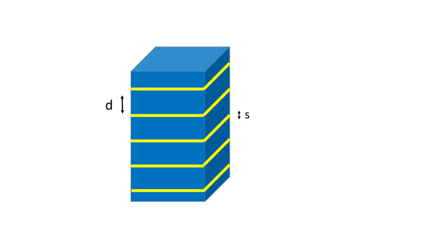
Figure 3: Layered Weyl semi - metal - a schematic picture.

Using the equilibrium value of the order parameter,

$$\Delta^{2}=\frac{f}{\beta}\tau,$$ (32)

the condensation energy density of an uniform superconductor (required in section V to describe thermal fluctuations’ importance) is

$$F_{s}=\int d^{3}r\text{ }D\left(\mu\right)\left[-\tau\left|\Delta\right|^{2}+\frac{\beta}{2f}\left|\Delta\right|^{4}\right]=-\frac{D_{0}\left(\mu\right)f\Delta^{2}\tau}{2}V=-\frac{D_{0}\left(\mu\right)f^{2}}{2\beta}\tau^{2}V.$$ (33)

Now we are ready to describe the magnetic properties of the superconductors.      

V GL in magnetic field. Comparison with experiment.

Effects of the external magnetic field are accounted for by the minimal substitution, $\mathbf{\nabla}\rightarrow\mathbf{D}=\mathbf{\nabla}-\frac{2ei}{c}\mathbf{A}$ in the GL equation Eq.(27) due to gauge invariance.  The GL equation in the presence of magnetic field allows the description of the magnetic response to homogeneous external field. We start from the strong field that destroys superconductivity.

V.1 Upper critical field.

The upper critical magnetic field $H_{c2}$ is as usual calculated from the liner part of the GL equation Eq.(27), as the lowest eigenvalue of the linear operator (including the magnetic field). Representing the homogeneous magnetic field in the Landau gauge, $A=H\left(-y,0,0\right)$,

one expands near $T_{c}$ as

$$H_{c2}\left(T\right)=H_{c2}\left(0\right)\tau,\$$ (34)

where the zero temperature intercept magnetic field is $H_{c2}\left(0\right)=\Phi_{0}/2\pi\xi_{x}\xi_{y}$. This is represented by  the dashed straight lines in Fig. 4. It is a product of the experimentally measured slope $\frac{dH_{c2}}{dT}|_{{}_{T=T_{c}}}$ and $T_{c}$:

$$H_{c2}\left(0\right)=\frac{\hbar cf}{2e\sqrt{C_{yy}C_{xx}}}.$$ (35)

In practice at very low temperature the mean field $H_{c2}\left(T\right)$ ”curved down”, so that actual upper field at zero temperature is about $60\%$ of that value. The GL model is not applicable that far from $T_{c}$.

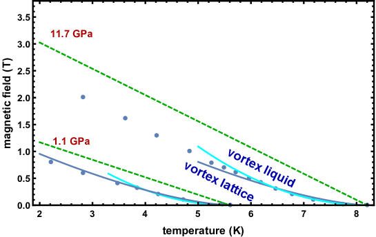
Figure 4: Magnetic phase diagram of layered WSM second kind superconductor. The experimental points are for $MoTe_{2}$ at pressures  $1.1GPa$ and $11.7GPa$ (blue). Upper critical field $H_{c2}\left(T\right)$ (”mean field”,dashed line) becomes a crossover due to thermal fluctuations.  At pressures $1.1$ and $11.7GPa$ the fitted curves are marked by the cyan lines for 3D and the blues line for 2D.

Measured upper critical field as function for parameter of $MoTe_{2}$ for two values of pressure, $1.1$ $GPa$ and $11.7$ $GPa$, is given as a red and blue points respectively line in Fig. 4. As will be discussed below, it will be interpreted as a melting line for the vortex lattice due to fluctuations. Vortex liquid phase in which the phase of the order parameter $\Delta$ is random appears between the melting line and the mean field line where order parameter disappears altogether.

Pressure determines the tilt parameter $\kappa$, which in turn influences $H_{c2}\left(0\right)$, as shown in Fig. 5 (blue lines). In the superconductor of the first kind it becomes the cooling field and is depicted as dashed lines at both small and large $\kappa$.

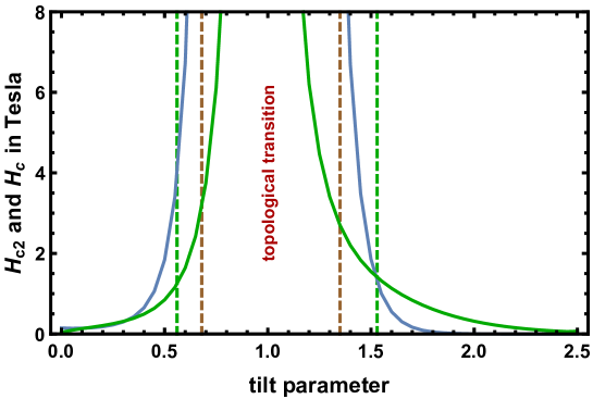
Figure 5: Upper critical field ($H_{c2}$, blue lines for type I and type II phases) and thermodynamic critical magnetic field ($H_{c}$, green) as a function on the tilt parameter. Brown dashed lines mark $T_{c}$ for two topological phases of $MoTe_{2}$.

V.2 Supercurrents and penetration depths in London limit.

V.2.1 Penetration depth.

Density of superconducting currents can be obtained by the variation of the free energy functional including the magnetic energy,

$$F=\int d^{3}r\left\{D_{0}\left(\mu\right)\left(C_{ii}\left|D_{i}\Delta\right|^{2}-f\tau\left|\Delta\right|^{2}+\frac{\beta}{2}\left|\Delta\right|^{4}\right)+\frac{\left(\nabla\times\mathbf{A}\right)^{2}}{8\pi}\right\}\text{,}$$ (36)

where $i=x,y,z$, with respect to components of the vector potential:

$$\mathbf{J}_{i}=D_{0}\left(\mu\right)\frac{2ei}{\hbar}C_{ii}\Delta\left(\mathbf{r}\right)D_{i}\Delta^{\ast}\left(\mathbf{r}\right)+c.c.\text{.}$$ (37)

Within the London approximation, in which the order parameter is approximated by $\Delta\left(\mathbf{r}\right)=\Delta e^{i\varphi}$, one obtains,

$$\mathbf{J}_{i}=\frac{4e}{\hbar}D_{0}\left(\mu\right)C_{ii}\Delta^{2}\left(\partial_{i}\varphi-\frac{2e}{c\hbar}A_{i}\right)\text{.}$$ (38)

Using the (in plane) Maxwell equations, one obtains the equation for a single Abrikosov vortex Keterson :

$$\lambda_{x}^{2}\left(T\right)\frac{\partial^{2}H}{\partial y^{2}}+\lambda_{y}^{2}\left(T\right)\frac{\partial^{2}H}{\partial x^{2}}-H=\frac{\Phi_{0}}{2\pi}\delta\left(x\right)\delta\left(y\right)\text{.}$$ (39)

The London penetration lengths in our case of layered WSM with parabolic dispersion relation along $z$ axis are:

$$\lambda_{x}^{2}\left(T\right)=\frac{c^{2}\hbar^{2}}{32\pi e^{2}D_{0}\left(\mu\right)C_{yy}\Delta^{2}}\text{.}$$ (40)

From the calculated coefficient of the cubic term of the GL equation and the Maxwell equation one obtains, after substitution of $D\left(\mu\right)$ from Eq.(31) and $\Delta$ from Eq.(32),

$$\lambda_{x}^{2}\left(0\right)=\frac{3\pi\hbar^{5}v^{2}c^{2}\beta}{32\sqrt{2}e^{2}m_{z}^{1/2}\mu^{3/2}C_{yy}f}\text{, }\lambda_{y}=\lambda_{x}/\varepsilon\text{.}$$ (41)

The quantities $\sqrt{2}\lambda_{x}\left(0\right)$ and $\sqrt{2}\lambda_{y}\left(0\right)$ are depicted in Fig.2a as dashed blue and green lines respectively. The factor $\sqrt{2}$ was introduced in order to mark the transitions from the first to second kind of superconductivity. For material parameters used in the present paper ($MoTe_{2}$) the transitions are reentrant in $\kappa$: $\kappa_{I}=0.53$ and $\kappa_{II}=1.5$ (intersection points with $\xi_{x}$ or consistently with $\xi_{y}$). The parameters that determine $m_{z}$ (see formula below Eq.(31)), are the interlayer distance $d=1.3nm$, the layer effective width $s=0.3nm$. The dependence is quite non-monotonic. At small $\kappa$ both penetration depths are large level off and increase slightly approaching $\kappa=1$. In the type II phase penetration depth largely decreases.

V.2.2 The Abrikosov parameter and transition between first and second kinds of superconductivity

The Abrikosov parameter is isotropic despite large anisotropies:

$$\kappa_{x}^{A}=\frac{\lambda_{x}}{\xi_{x}}=\frac{vc}{8e}\sqrt{\frac{3\sqrt{2}\pi\hbar^{5}\beta}{m_{z}^{1/2}\mu^{3/2}C_{xx}C_{yy}}}=\kappa_{y}^{A}\ \text{.}$$ (42)

This is plotted against the tilt parameter in Fig. 6. The green line is the universal critical value $\kappa_{x}^{A}=1/\sqrt{2}$ for the above mentioned transitions between the first and the second kind superconductivity.

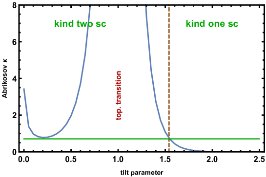
Figure 6: Abrikosov parameter of the WSM superconductor as function of $\kappa$. The green line is the universal critical value $\kappa_{x}^{A}=1/\sqrt{2}$for the transitions between the first and the second kind superconductivity.

Thermodynamic critical field for kind I superconductors is given by

$$H_{c}^{2}\left(0\right)=8\pi F_{s}=4\pi D_{0}\left(\mu\right)f\Delta^{2}=\frac{4\sqrt{2m_{z}}\mu^{3/2}f^{2}}{3\pi\hbar^{3}v^{2}\beta}\text{,}$$ (43)

where the condensation energy was given in Eq.(33). It is plotted as dashed lines in Fig.5 as dashed lines.

V.3 The Abrikosov vortex solution and the lower critical field.

In a hard type-II superconductor magnetic field screened the Abrikosov vortex obeyed the equation Eq.(39). This equation has a well known anisotropic Abrikosov vortex solutionKeterson :

$$H\left(x,y\right)=\frac{\Phi_{0}}{2\pi\lambda_{x}\lambda_{y}}K_{0}\left[\left(\frac{y^{2}}{\lambda_{x}^{2}}\ +\frac{x^{2}}{\lambda_{y}^{2}}\right)^{1/2}\right]\text{.}$$ (44)

here $K_{0}$ is the modified Bessel function.

Abrikosov vortex in WSM appears at lower critical field

$$H_{c1}\left(0\right)=\frac{\Phi_{0}}{2\pi\lambda_{x}\lambda_{y}}\ln\left[\kappa^{A}\right]\text{.}$$ (45)

The material parameters calculated above allow determination of the strength of thermal fluctuations that might be significant in thin films as seen from the nonlinear concave shape of measuredMoTe2melting transition field dependence on temperature near $T_{c}$ in $MoTe_{2}$ superconductor, see Fig. 4. However the experimental points of the magnetic $H_{c2}$ (blue dots in Fig.4) indicate that the mean field description breaks down near $T_{c}$. This will be explained next as a thermal fluctuations effect.

VI Ginzburg criterion for strong thermal fluctuations region.

The thermal fluctuations were neglected so far. In this section they are taken into account in the framework of the GL energy. Here one cannot ignore the fluctuations of the order parameter in direction perpendicular to the layer, since magnetic field couples the layers via the ”pancake vortices” interactionRMP .

VI.1 Ginzburg number in layered superconductor

The fluctuation contribution to the heat capacity (per volume) that is most singular in $\tau=1-T/T_{c}$ isPatashinsky ; Landau :

$$C_{fluct}=\frac{\pi^{2}}{\xi_{x}\xi_{y}\xi_{z}}\frac{1}{\sqrt{\tau}}\text{.}$$ (46)

It should be compared with the mean field heat capacity $C_{mf}$ in the superconducting phase (see Eqs.(32) and (31):

$$C_{mf}=\frac{D_{0}\left(\mu\right)f^{2}}{\beta T_{c}}=\frac{\sqrt{2m_{z}}\mu^{3/2}}{3\pi^{2}\hbar^{3}v^{2}}\frac{f^{2}}{\beta T_{c}}\text{.}$$ (47)

The ratio,

$$\frac{C_{fl}}{C_{mf}}=\frac{3\pi^{4}\hbar^{3}v^{2}}{\sqrt{2m_{z}\mu^{3}f}}\frac{\beta T_{c}}{\sqrt{C_{xx}C_{yy}C_{zz}}}\frac{1}{\sqrt{\tau}}\text{,}$$ (48)

characterizes the fluctuation strength. Strong fluctuations effects appear in the temperature region where $C_{fl}>C_{mf}$. The temperature independent Levanyuk - Ginzburg number is defined by:

$$Gi^{th}=\frac{9\pi^{8}\hbar^{6}v^{4}}{2m_{z}\mu^{3}}\frac{\beta^{2}T_{c}^{2}}{C_{xx}C_{yy}C_{zz}f}\text{.}$$ (49)

The Ginzburg number is plotted as function of $\kappa$ in Fig.7. for parameters pertinent to an experimentMoTe2melting in $MoTe_{2}$. In this case $Gi$ ranges between relatively large values in Type I WSM phase $\kappa$ close to the topological transition line and small $Gi$ value in Type II WSM phase. In type I phase there exists a minimum. Significant thermal fluctuations lead to melting of the Abrikosov flux lattice to the vortex liquid. Values of $Gi$ for $MoTe_{2}$ at pressures $1.1GPa$ and $11.7GPa$ clearly exhibiting the melting lineMoTe2melting are given in Table 1.

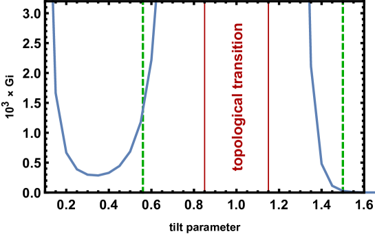
Figure 7: Gi number characterizing the strength of thermal fluctuations as function of the tilt parameter $\kappa.$

VI.2 Abrikosov lattice melting line

It was shownRosenstein02 that the melting line is determined for 3D and 2D thermal fluctuationsshapiro88 by

$$-a_{T}^{3D} = 2^{1/3}\left(th\right)^{-2/3}Gi^{-1/3}\left(1-t-h\right)=9.5;$$ (50)

$$-a_{T}^{2D} = 2^{-1/4}\left(th\right)^{-1/2}Gi^{-1/4}\left(1-t-h\right)=13.2,$$

respectively. Here the scaled melting field, see Fig. 4, is $h=H/H_{c2}\left(0\right)\$ and $t=T/T_{c}$. The values of Thouless parameter RMP at the first order melting transition were determined by comparing energies of the vortex solid and liquid found nonperturbatively.

In the vicinity of $T_{c}$, namely for $h,1-t<<1$, the expression for the melting field simplifies $H_{m}^{D}\left(T\right)=H_{m}^{D}\left(1-t\right)^{3-D/2}$ with values of $H_{m}^{D}$ given by

$$H_{m}^{2} = \frac{1}{\left(13.2\right)^{2}\sqrt{2Gi_{2}}}H_{c2}\left(0\right)$$ (51)

$$H_{m}^{3} = \frac{\sqrt{2}}{\left(9.5\right)^{3/2}\sqrt{Gi_{3}}}H_{c2}\left(0\right)$$

In our case of $MoTe_{2}$ at pressures $1.1$ and $11.7GPa$ the fitted constants (see the cyan lines for 3D and the blue lines for 2D in Fig.4), one obtains the best fits for $H_{m}^{D}$ given in Table 1.

Table 1: Fitting parameters for $H_{m}^{D}$

pressure	$T_{c}$	$\kappa$	$H_{c2}\left(0\right)$	$\xi_{x}$	$\lambda_{x}$	$H_{m}^{2}$	$H_{m}^{3}$	$Gi^{2Dfit}$	$Gi^{3Dfit}$	$Gi^{th}$
1.1GPa	5.6	1.5	1.5T	18nm	20nm	3.5T	1.85T	3$\cdot 10^{-6}$	$1.5\cdot 10^{-3}$	$2.7\cdot 10^{-5}$
11.7GPa	8.2K	0.53	4T	10nm	40nm	7.2T	3.3T	$5\cdot 10^{-6}$	$3.4\cdot 10^{-3}$	$1.3\cdot 10^{-3}$

The $Gi$ in both cases was determined from the several experimental points close to $T_{c}$ using

$$Gi^{D} = c_{D}\left(H_{c2}\left(0\right)/H_{m}\right)^{2};$$ (52)

$$c_{2} = 1.64\cdot 10^{-5};c_{3}=2.33\cdot 10^{-3}\text{.}$$

while $Gi^{th}$ is calculated in Eq.(49).

The actual melting line significantly below $T_{c}$ typically bends down and cannot be obtained within the GL expansion. The theoretical value in the table is taken from Fig.7.

VII Conclusion and discussion.

Magnetic properties of Weyl semi - metals turned superconductors at low temperatures were derived from a microscopic phonon mediated multi - band pairing model via the Ginzburg - Landau effective theory for the (singlet) order parameter. The Gorkov approach was used to determine microscopically anisotropic coherence length, the penetration depth, Fig.2a, determining the Abrikosov parameter for a layered material. It is shown that very strong in plane anisotropy is caused by the tilt of Dirac cones, see Fig. 2b. It is found that generally that superconductivity is strongly second kind (penetration depth much larger than coherence length) near the WSM topological transition (tilt parameter $\kappa=1$, see Fig. 6), but becomes first kind away from it especially in type II WSM. This possibility has been observed recently in similar materialPdTe2TypeI $PaTe_{2}$.

For WSM superconductors of the second kind the dependence of the upper and lower critical fields $H_{c2}\left(T\right)$ and $H_{c1}\left(T\right)$ on the tilt parameter $\kappa$ (governed by pressure, see Fig. 5) was obtained from the GL energy not very far from $T_{c}$ (where the GL approach is valid). In WSM superconductors of first kind the relevant fields are the thermodynamic field $H_{c}\left(T\right)$ and $H_{c2}\left(T\right)$ that takes a role of the supercooling field. In strongly layered WSM superconductors the mean field GL approach is not sufficient due to thermal fluctuations despite relatively low critical temperatures.

Strength of thermal fluctuations is estimated generally and its is found that they are strong enough in strongly layered materials to cause Abrikosov vortex melting. Moreover we predict that, while for type I WSM the fluctuations of the layered material in magnetic field are three dimensional, they become two dimensional in the type II phase. Results are well fitted (see Fig. 4) by general melting line formulas derived within the lowest Landau level GL approach.

Main results of the paper are applied to the layered WSM superconductor $MoTe_{2}$. Magnetic properties of this material were extensively studiedMoTe2melting under pressures from ambient to $30GPa$. In this system the superconducting critical temperature has maximum at the pressure about $12GPa$. While the theory naively predicts Zyuzin ; Rosenstein17 sharp rise of $T_{c}$ at the topological transition between Type I and Type II phases of WSM, the region of maximum is beyond the range of its validity (see Fig.1, with dashed red lines indicating the range). We believe however that two values of pressure at which magnetic properties were comprehensively measured belong to different phases of WSM. Non-linear shape of the transition line to the normal state at temperatures below $T_{c}$ , see Fig.4, might be explained either by strong fluctuations in the vortex matter of the second kind superconductor or by spatial inhomogeneity on the mesoscopic scale. We argue that the first option is more likely, since the line clearly has a power dependence on temperature near $T_{c}$.

Our results support a view expressed in ref. MoTe2melting that magnetic properties of this dichalcogenides are reminiscent of those of  the well studied ”conventional” layered superconductor $NbSe_{2}$ (perhaps this is related to the fact that the later also possesses a pronounced multi - band electronic structure). It is expected that similar materials exhibit phenomena described theoretically here. In particular it was observed very recently PdTe2TypeI that in a dichalcogenides $PdTe_{2}$ $T_{c}$decreases slowly with pressure. In this material the pair of type-II Dirac points disappears at $6.1$ $GPa$, while a new pair of type-I Dirac points emerges at $4.7$ $GPa$. Therefore the theoretical analysis of this material is complicated by the fact that for $4.7-6.1$ $GPa$, the type-II and type-I Dirac cones coexist PdTe2 . The superconductor $PdTe_{2}$ was recently classified as a Type II Dirac semimetal with magnetic measurements confirmed that $PdTe_{2}$ was a first kind superconductor with $T_{c}=1.64$ $K$ and the thermodynamic critical field of $H_{c}(0)$ $=13.6$ $mT$ (intermediate state under magnetic field is typical to a first kind superconductor, as demonstrated by the differential paramagnetic effect PdTe2TypeI ).

This feature is consistent with the magnetic phase diagram of the present paper, where the first kind superconductivity is predicted in the Type-II phase of the WSM (see Fig. 4).

The calculation was limited to strongly layered case. The usage of continuum 3D model instead of fully layered Lawrence - DoniachLD model is justified in the present case while. The calculation can be extended to arbitrary tunneling strength and is in progress.

Acknowledgements.

We are grateful to T. Maniv, W. B. Jian, N.L. Wang for valuable discussions. B.R. was supported by NSC of R.O.C. Grants No. 103-2112-M-009-014-MY3 and is grateful to School of Physics of Peking University and Bar Ilan Center for Superconductivity for hospitality. The work of D.L. also is supported by National Natural Science Foundation of China (No. 11274018 and No. 11674007).

Appendix A Gorkov equations in integral form

Gorkov equations Eq.(4) can be presented in an integral form:

$$g_{\epsilon\kappa}\left(\mathbf{r,r}^{\prime}\ \omega\right)=\mathrm{g}_{\epsilon\kappa}^{1}\left(\mathbf{r}-\mathbf{r}^{\prime},\omega\right)-\int\mathrm{g}_{\epsilon\theta}^{1}\left(\mathbf{r}-\mathbf{r}^{\prime\prime},\omega\right)\Delta_{\theta\phi}^{\ast}\left(\mathbf{r}^{\prime\prime}\right)f_{\phi\kappa}^{+}\left(\mathbf{r}^{\prime\prime}\mathbf{,r}^{\prime},\omega\right);$$ (53)

$$f_{\beta\kappa}^{+}\left(\mathbf{r,r}^{\prime},\omega\right)=\int\mathrm{g}_{\beta\alpha}^{2}\left(\mathbf{r-r}^{\prime\prime\prime},-\omega\right)\Delta_{\alpha\epsilon}^{\ast}\left(\mathbf{r}^{\prime\prime\prime}\right)\left[\mathrm{g}_{\epsilon\kappa}^{1}\left(\mathbf{r}^{\prime\prime\prime}-\mathbf{r}^{\prime},\omega\right)-\int\mathrm{g}_{\epsilon\theta}^{1}\left(\mathbf{r}^{\prime\prime}-\mathbf{r}^{\prime\prime\prime},\omega\right)\Delta_{\theta\phi}^{\ast}\left(\mathbf{r}^{\prime\prime}\right)f_{\phi\kappa}^{+}\left(\mathbf{r}^{\prime\prime}\mathbf{,r}^{\prime},\omega\right)\right]$$ (54)

Expanding in small order parameter $\Delta,$ one obtains Eq.9 :

$$\Delta\left(\mathbf{r}\right) = \frac{g^{2}T}{2}\sum\limits_{\omega}\int\left[\begin{array}[]{c}\left[\mathrm{g}_{21}^{2}\left(\mathbf{r-r}^{\prime\prime\prime}\right)\mathrm{g}_{21}^{1}\left(\mathbf{r}^{\prime\prime\prime}-\mathbf{r}\right)\right]\sigma_{12}^{x}\sigma_{12}^{x}+\left[\mathrm{g}_{11}^{2}\left(\mathbf{r-r}^{\prime\prime\prime}\right)\mathrm{g}_{22}^{1}\left(\mathbf{r}^{\prime\prime\prime}-\mathbf{r}\right)\right]\sigma_{21}^{x}\sigma_{12}^{x}+\\ \left[\mathrm{g}_{12}^{2}\left(\mathbf{r-r}^{\prime\prime\prime}\right)\mathrm{g}_{12}^{1}\left(\mathbf{r}^{\prime\prime\prime}-\mathbf{r}\right)\right]\sigma_{21}^{x}\sigma_{21}^{x}+\left[\mathrm{g}_{22}^{2}\left(\mathbf{r-r}^{\prime\prime\prime}\right)\mathrm{g}_{11}^{1}\left(\mathbf{r}^{\prime\prime\prime}-\mathbf{r}\right)\right]\sigma_{12}^{x}\sigma_{21}^{x}\end{array}\right]\Delta\left(\mathbf{r}^{\prime\prime\prime}\right)$$

$$-\int\mathrm{g}_{\beta\alpha}^{2}\left(\mathbf{r-r}^{\prime\prime\prime}\right)\mathrm{g}_{\epsilon\theta}^{1}\left(\mathbf{r}^{\prime\prime}-\mathbf{r}^{\prime\prime\prime}\right)\mathrm{g}_{\phi\zeta}^{2}\left(\mathbf{r}^{\prime\prime}\mathbf{-r}_{3}\right)\mathrm{g}_{\epsilon\kappa}^{1}\left(\mathbf{r}_{3}-\mathbf{r}\right)\Delta_{\theta\phi}^{\ast}\left(\mathbf{r}^{\prime\prime}\right)\Delta_{\alpha\epsilon}^{\ast}\left(\mathbf{r}^{\prime\prime\prime}\right)\Delta_{\zeta\epsilon}^{\ast}\left(\mathbf{r}_{3}\right)$$

Appendix B Calculation of the normal GF

Normal Green function obeyed the equations 5,8. First four GF are calculated from the equation

$$L_{\gamma\beta}^{1}\mathrm{g}_{\beta\kappa}^{1}\left(\mathbf{r-r}^{\prime}\right)=\delta^{\gamma\kappa}\delta\left(\mathbf{r-r}^{\prime}\right),$$ (58)

where $L_{\gamma\beta}^{1}=\left[\left(i\omega+\mu+i\mathbf{w\nabla}_{r}\right)\delta_{\gamma\beta}+\left(-iv\sigma_{\gamma\beta}^{i}\ \nabla_{r}^{i}\right)\right]$ by performing Fourier transform for different pseudo-spin indexes. In particular for $\gamma=1,\kappa=1\$it reads in momentum representation

$$\ \left(i\omega+\mu-\mathbf{wp}\right)g_{11}^{1}\left(\mathbf{p}\right)+v\left(\ \mathbf{p}^{x}-i\ \mathbf{p}^{y}\right)g_{21}^{1}\left(\mathbf{p}\right) = 1;$$ (59)

$$\left(i\omega+\mu-\mathbf{wp}\right)g_{11}^{1}\left(\mathbf{p}\right)+vp\left(\ \cos\varphi-i\sin\varphi\right)g_{21}^{1}\left(\mathbf{p}\right) = 1.$$

The rest of the normal GF may be obtained by the same method. The second group of the normal Green functions obey the equations $L_{\gamma\beta}^{2}g_{0\beta\kappa}^{2}\left(\mathbf{r-r}^{\prime}\right)=\delta^{\gamma\kappa}\delta\left(\mathbf{r-r}^{\prime}\right)\$with $L_{\gamma\beta}^{2}$ defined in Eq.(5) are obtained by the same method.

The GF obtained after solution of these equations are:

$$g_{22}^{1}\left(\mathbf{p}\right) = z^{\ast-1}\left(i\omega+\mu-\mathbf{wp}\right);\text{ \ }g_{12}^{1}\left(\mathbf{p}\right)=-z^{\ast-1}vpe^{-i\varphi}$$ (60)

$$g_{11}^{1}\left(\mathbf{p}\right) = z^{\ast-1}\left(i\omega+\mu-\ \mathbf{wp}\right);\text{ }g_{21}^{1}\left(\mathbf{p}\right)=-z^{\ast-1}vpe^{i\varphi}$$

$$g_{11}^{2}\left(\mathbf{p}\right)\ = z^{-1}\ \left(-i\omega+\mu-\mathbf{wp}\right);\text{ }g_{12}^{2}\left(\mathbf{p}\right)=-z^{-1}vpe^{i\varphi}$$

$$g_{22}^{2}\left(\mathbf{p}\right) = z^{-1}\left(-i\omega+\mu-\ \mathbf{wp}\right);\text{ \ }g_{21}^{2}\left(\mathbf{p}\right)=-z^{-1}vpe^{-i\varphi}\ ;$$

$$z = \left(-i\omega+\mu-\mathbf{wp}\right)^{2}-\left(vp\right)^{2},$$

where $\mathbf{p}$ is the 2D momentum and $\varphi$ is the azimuthal angle in the $p_{x},p_{y}$ plane.

Appendix C The critical temperature and the linear term in GL expansion.

C.1 The critical temperature for 2D case.

The linear terms in the GL expansion read:

$$a\left(T\right)=T\sum\nolimits_{\omega,\mathbf{p}}a\left(\mathbf{p}\right)-\frac{1}{g^{2}},$$ (61)

with

$$a\left(\mathbf{p}\right)=2\ Z^{-1/2}\left(\left(vp\right)^{2}\ +\ \ \omega^{2}+\left(\mu-w_{x}p_{x}\right)^{2}\right)\ \text{.}$$ (62)

Here $Z$ is defined in Eq.(19). Performing the summation over $\omega_{n}$, one obtains,

$$a\left(T\right)\ \ =\frac{1}{4\left(2\pi\right)^{2}\ }\int_{\theta=0}^{2\pi}\int_{p}\Theta\left(-\varepsilon+\mu+\Omega\right)\Theta\left(\varepsilon-\mu+\Omega\right)\left\{\frac{p\tanh\left[\frac{\left|p\left(1+w\cos\theta\right)-\mu\right|}{2T}\right]}{\left|p\left(1+w\cos\theta\right)-\mu\right|}+\frac{p\tanh\left[\frac{\left|p\left(1+w\cos\theta\right)+\mu\right|}{2T}\right]}{\left|p\left(1+w\cos\theta\right)+\mu\right|}\right\}-\frac{1}{g^{2}}\text{.}$$ (63)

Introducing new variables:

$$\varepsilon\left(p,\theta\right)=vp+wp_{x}=p\left(1+w\cos\theta\right);E=vp\left(1+w\cos\theta\right)-\mu,$$ (64)

one obtains

$$a\left(T\right)=\frac{\mu}{8\pi v^{2}}f\left(\kappa\right)\left\{2\left(\log\frac{\Omega}{2T}\text{ }\tanh\left[\frac{\Omega}{2T\ }\right]-\int_{\varepsilon=0}^{\Omega}d\varepsilon\frac{\log\varepsilon}{\cosh^{2}\left[\frac{\varepsilon}{2T}\right]}\right)+\frac{\Omega}{\mu}\right\}-\frac{1}{g^{2}}\text{.}$$ (65)

In the adiabatic approximation, $\mu>>\Omega$ it gives for coefficients $a\left(T\right)$ and the critical temperature $T_{c}$, Eqs.(20,21).

Appendix D Gradient terms C_ik and cubic term

In this Appendix the gradient terms in the GL expansion are calculated.

D.1 Diagonal gradient terms for 2D case.

Gradient terms in the GL expansion has the form of (15). Substituting the normal GF from Eq. (60), one obtains after a simple calculations the diagonal gradient terms. In Cartesian coordinate (with cone vector $w$ is directed along the $x$ axes) the tensor $C_{ki}$ is diagonal while $C_{xy}$ and $C_{yx}$ are zero due to the reflection symmetry in the $y$ direction). The diagonal components are

$$C_{xx}\left(w,\mathbf{p}\right)=\frac{1}{2Z}\left\{\begin{array}[]{c}v^{2}\left(2p_{x}w_{x}\mu-2p_{x}^{2}w_{x}^{2}-2w_{x}\omega p_{y}+v^{2}p_{x}^{2}-\omega^{2}+\left(\mu-w_{x}p_{x}\right)^{2}-v^{2}p_{y}^{2}\right)^{2}\\ +v^{2}\left(2p_{x}w_{x}\mu-2p_{x}^{2}w_{x}^{2}+2p_{y}w_{x}\omega+2v^{2}p_{x}^{2}-\omega^{2}+\left(\mu-w_{x}p_{x}\right)^{2}-\left(vp\right)^{2}\right)^{2}\\ +4v^{2}\left(w_{x}^{2}p_{x}p_{y}-\mu w_{x}p_{y}-p_{y}p_{x}v^{2}-\omega\mu\right)^{2}+4v^{2}\left(-w_{x}p_{x}p_{y}w_{x}+p_{y}\mu w_{x}+p_{y}p_{x}v^{2}-\omega\mu\right)^{2}\\ +2\left(-\omega^{2}w_{x}+w_{x}\left(\mu-w_{x}p_{x}\right)^{2}+2v^{2}p_{x}\left(\mu-w_{x}p_{x}\right)+w_{x}\left(vp\right)^{2}\right)^{2}+8\left(\omega w_{x}\left(\mu-w_{x}p_{x}\right)+v^{2}p_{x}\omega\right)^{2}\end{array}\right\};$$ (66)

$$C_{yy}\left(w,\mathbf{p}\right)=\frac{1}{Z}\left\{\begin{array}[]{c}v^{2}\left(\omega^{2}-2v^{2}p_{y}^{2}-\left(\mu-w_{x}p_{x}\right)^{2}+\left(vp\right)^{2}\right)^{2}\\ +v^{2}\left[4\left(\left(v^{2}p_{y}p_{x}\right)^{2}+\omega^{2}\left(\mu-w_{x}p_{x}\right)^{2}\right)\right]+4\left(v^{2}p_{y}\right)^{2}\left(\omega^{2}+\left(\mu-w_{x}p_{x}\right)^{2}\right)\end{array}\right\}\text{.}$$ (67)

D.2 Gradient terms and effective coherent lengths for 2D layer

After integration over momenta $p$ and the azimuthal angle $\varphi$ in the second term in equation Eq.(13) can be performed numerically using the dimensionless variables

$$E=\kappa\epsilon\cos\varphi+\epsilon;\epsilon=\frac{E}{\kappa\cos\varphi+1}=\left(E\psi\right);\psi\left(\kappa,\varphi\right)\ =\frac{1}{\left(\kappa\cos\varphi+1\right)};,$$ (68)

where

$$x=-\overline{\mu}+E\epsilon=\frac{vp}{T_{c}},\overline{\mu}=\frac{\mu}{T_{c}},\overline{\omega}=\frac{\omega}{T_{c}}$$ (69)

As a result one obtains the gradient terms coefficients which are proportional to the square of the anisotropic coherence lengths depending on ratio $\kappa=w/v.$

$$\eta_{y} = \frac{1}{2\pi\overline{\mu}\ }\sum\limits_{\omega}\int\left(x+\overline{\mu}\right)dxd\varphi\cdot sign\left[\kappa\cos\varphi+1\right]\left\{\left(\kappa\cos\varphi+1\right)\left(\overline{\omega}^{2}+x^{2}\right)\left(\overline{\omega}^{2}+\left(-x+2\left(x+\overline{\mu}\right)\psi\left(\kappa,\varphi\right)\right)\right)\right\}^{-2}$$ (73)

$$\times\left\{\begin{array}[]{c}\left[\overline{\omega}^{2}+\left(\overline{\mu}-\kappa\left(x+\overline{\mu}\right)\psi\left(\kappa,\varphi\right)\cos\varphi\right)^{2}\right]^{2}-4\left(x+\overline{\mu}\right)^{2}\psi^{2}\left(\kappa,\varphi\right)\cos 2\varphi\left(\overline{\mu}-\left(x+\overline{\mu}\right)\kappa\psi\left(\kappa,\varphi\right)\cos\varphi\right)^{2}\\ +\left(x+\overline{\mu}\right)^{4}\psi^{4}\left(\kappa,\varphi\right)+2\left(x+\overline{\mu}\right)^{2}\psi^{2}\left(\kappa,\varphi\right)\overline{\omega}^{2}+2\left(x+\overline{\mu}\right)^{2}\psi^{2}\left(\kappa,\varphi\right)\left(\overline{\mu}-\left(x+\overline{\mu}\right)\kappa\psi\left(\kappa,\varphi\right)\cos\varphi\right)^{2}\end{array}\right\}$$

and

$$\eta_{x} = \frac{1}{4\pi\overline{\mu}}\sum\limits_{\omega}\int\left(x+\overline{\mu}\right)dxd\varphi\frac{sign\left(\left(\kappa\cos\varphi+1\right)\right)\left(\overline{\omega}^{2}+\left(-x+2\left(x+\overline{\mu}\right)\psi\left(\kappa,\varphi\right)\right)^{2}\right)^{-2}}{\left(\kappa\cos\varphi+1\right)^{2}\left(\overline{\omega}^{2}+x^{2}\right)^{2}}\times$$ (85)

$$\times\left[\begin{array}[]{c}\left(\begin{array}[]{c}2\kappa\ \overline{\mu}\left(x+\overline{\mu}\right)\psi\cos\varphi-2\left(x+\overline{\mu}\right)^{2}\psi^{2}\kappa_{\ }^{2}\cos^{2}\varphi-2\kappa\ \overline{\omega}\left(x+\overline{\mu}\right)\psi\sin\varphi\\ +\left(x+\overline{\mu}\right)^{2}\psi^{2}\cos 2\varphi-\overline{\omega}^{2}+\left(\overline{\mu}-\kappa\left(\left(x+\overline{\mu}\right)\psi\right)\cos\varphi\right)^{2}\end{array}\right)^{2}+\\ \ \left(\begin{array}[]{c}2\kappa\ \overline{\mu}\left(x+\overline{\mu}\right)\psi\cos\varphi-2\kappa_{\ }^{2}\left(\left(x+\overline{\mu}\right)\psi\right)^{2}\cos^{2}\varphi+2\kappa\left(x+\overline{\mu}\right)\psi\overline{\omega}\sin\varphi\\ +\left(\left(x+\overline{\mu}\right)\psi\right)^{2}\cos^{2}\varphi-\overline{\omega}^{2}+\left(\overline{\mu}-\kappa\left(x+\overline{\mu}\right)\psi\cos\varphi\right)^{2}-\left(\left(x+\overline{\mu}\right)\psi\right)^{2}\sin^{2}\varphi\end{array}\right)^{2}\\ +4\ \left(\kappa_{\ }^{2}\left(\left(x+\overline{\mu}\right)\psi\right)^{2}\sin\varphi\cos\varphi-\kappa\overline{\mu}\left(\left(x+\overline{\mu}\right)\psi\right)\sin\varphi-\left(\left(x+\overline{\mu}\right)\psi\right)^{2}\sin\varphi\cos\varphi-\overline{\omega}\overline{\mu}\right)^{2}\\ +4\ \left(-\kappa^{2}\left(\left(x+\overline{\mu}\right)\psi\right)^{2}\sin\varphi\cos\varphi\ +\kappa\overline{\mu}\left(\left(x+\overline{\mu}\right)\psi\right)\sin\varphi\ +\left(\left(x+\overline{\mu}\right)\psi\right)^{2}\sin\varphi\cos\varphi-\overline{\omega}\overline{\mu}\right)^{2}\\ +2\ \left(-\overline{\omega}^{2}\kappa\ +\ \kappa\ \left(\overline{\mu}-\kappa\left(x+\overline{\mu}\right)\psi\cos\varphi\right)^{2}+2\left(x+\overline{\mu}\right)\psi\cos\varphi\left(\overline{\mu}-\kappa\left(x+\overline{\mu}\right)\psi\cos\varphi\right)+\kappa\left(\left(x+\overline{\mu}\right)\psi\right)^{2}\right)^{2}\\ +8\ \left(\kappa\overline{\omega}\ \left(\overline{\mu}-\kappa\left(\left(x+\overline{\mu}\right)\psi\right)\cos\varphi\right)+\overline{\omega}\left(x+\overline{\mu}\right)\psi\cos\varphi\right)^{2}\end{array}\right]$$

The results are presented in Eq.(24) in the text.

D.3 Cubic Term in GL Expansion

Substituting GF into Eq.(25) in text one obtains:

$$b\left(\mathbf{p}\right)=\frac{2\ \left[\left(vp\right)^{2}\ +\omega^{2}+\left(\mu-wp_{x}\right)^{2}\right]\left[\left(vp\right)^{2}\ +\omega^{2}+\left(\mu+wp_{x}\right)^{2}\right]}{\left[\ \omega^{2}+\left(\mu-wp_{x}-vp\right)^{2}\right]\left[\ \omega^{2}+\left(\mu-wp_{x}+vp\right)^{2}\right]\left[\omega^{2}+\left(\mu+wp_{x}-vp\right)^{2}\right]\left[\ \omega^{2}+\left(\mu+wp_{x}+vp\right)^{2}\right]}$$ (86)

and after integration over momentum the result is Eq.(25) with

$$\ \eta=\sum\limits_{\omega}\int_{\varphi}^{2\pi}\int_{x=0}^{\infty}\left(x+\overline{\mu}\right)\frac{sign\left[\kappa\cos\varphi+1\right]}{\left(\kappa\cos\varphi+1\right)^{2}}\times$$ (87)

$$\times\frac{\left\{\left[\left(x+\overline{\mu}\right)\psi\right]^{2}\ +\overline{\omega}^{2}+\left(\overline{\mu}-\kappa\left(x+\overline{\mu}\right)\psi\cos\varphi\right)^{2}\right\}\left\{\left[\left(x+\overline{\mu}\right)\psi\right]^{2}\ +\overline{\omega}^{2}+\left(\overline{\mu}+\kappa\left(x+\overline{\mu}\right)\psi\cos\varphi\right)^{2}\right\}}{\ \left\{\overline{\omega}^{2}+\left(\overline{\mu}-\kappa\left(x+\overline{\mu}\right)\psi\cos\varphi-\left(x+\overline{\mu}\right)\psi\right)^{2}\right\}\ \left\{\overline{\omega}^{2}+\left(\overline{\mu}-\kappa\left(x+\overline{\mu}\right)\psi\cos\varphi+\left(x+\overline{\mu}\right)\psi\right)^{2}\right\}}.$$

This was evaluated numerically.

D.4
Gradient term in direction perpendicular to layers

In this case the set of the 3D GF is transformed has the presented in the form 60 where $\mu$ is replaced by $\mu-\frac{p_{z}^{2}}{2m_{z}}.$ Substituting the modified 3D GF into Eq.(15) one obtains

$$C_{zz} = \frac{g^{2}Ts}{2\left(2\pi\hbar\right)^{3}}\sum\limits_{\omega}\int_{\mathbf{p}}\frac{p_{z}^{2}}{m_{z}^{2}}\Theta\left(vp+\frac{p_{z}^{2}}{2m_{z}}-\Omega-\mu+wp_{x}\right)\Theta\left(vp+\frac{p_{z}^{2}}{2m_{z}}+\Omega-\mu+wp_{x}\right)$$

$$\frac{4v^{2}p^{2}\ \left[\omega^{2}+\left(\mu-\frac{p_{z}^{2}}{2m_{z}}-wp_{x}\right)^{2}\right]+\left[\omega^{2}+\left(\mu-\frac{p_{z}^{2}}{2m_{z}}-wp_{x}\right)^{2}\right]^{2}+2\left(\mu-\frac{p_{z}^{2}}{2m_{z}}-wp_{x}\right)^{2}\left(vp\right)^{2}+\left(vp\right)^{4}}{\left[\ \omega^{2}+\left(\mu-\frac{p_{z}^{2}}{2m_{z}}-wp_{x}-vp\right)^{2}\right]^{2}\left[\ \omega^{2}+\left(\mu-\frac{p_{z}^{2}}{2m_{z}}-wp_{x}+vp\right)^{2}\right]^{2}}\text{,}$$

where $\Theta\left(x\right)$ is the theta function restricting the integration area in the Debye shell at the Fermi energy.

Introducing dimensionless variable by

$$\varepsilon=vp/T;\varepsilon_{z}=\frac{p_{z}^{2}}{2m_{z}T};p_{z}=\sqrt[\ ]{2m_{z}T\varepsilon_{z}}\text{,}$$ (89)

the coefficient in Eq.(29) takes a form:

$$\eta_{z} = \sum\limits_{\omega}\int\sqrt{\varepsilon_{z}}d\varepsilon_{z}\varepsilon d\varepsilon d\varphi\Theta\left(\varepsilon+\varepsilon_{z}+\overline{\Omega}-\overline{\mu}\right)\Theta\left(\varepsilon+\varepsilon_{z}-\overline{\Omega}-\overline{\mu}\right)$$

$$\frac{4\varepsilon^{2}\ \left[\overline{\omega}^{2}+\left(\overline{\mu}-\varepsilon_{z}-\kappa\varepsilon\cos\varphi\right)^{2}\right]+\left[\overline{\omega}^{2}+\left(\overline{\mu}-\varepsilon_{z}-\kappa\varepsilon\cos\varphi\right)^{2}\right]^{2}+2\left(\overline{\mu}-\varepsilon_{z}-\kappa\varepsilon\cos\varphi\right)^{2}\varepsilon^{2}+\varepsilon^{4}}{\left\{\left[\ \overline{\omega}^{2}+\left(\overline{\mu}-\varepsilon_{z}-\kappa\varepsilon\cos\varphi-\varepsilon\right)^{2}\right]\left[\ \overline{\omega}^{2}+\left(\overline{\mu}-\varepsilon_{z}-\kappa\varepsilon\cos\varphi+\varepsilon\right)^{2}\right]\right\}^{2}}\text{.}$$

This equation was evaluated numerically and results presented in Fig. 2c.

Appendix E Density of states in WSM.

In this Appendix we calculate the DOS for the normal electrons described by the Hamiltonian (1). Using the dispersion relation for a single electron,

$$E=\varepsilon+\varepsilon_{z}+\varepsilon\kappa\cos\varphi,$$ (91)

one obtains for electron density (for two sublattices and two spins)

$$n=\frac{4}{\left(2\pi\right)^{3}\hbar^{3}}\int_{p}\varepsilon d\varepsilon d\varphi dp_{z}\Theta\left(E\left[\varepsilon,p\right]-\mu\right)\text{,.}$$ (92)

The DOS is

$$\frac{dn}{d\mu}=\frac{4}{\left(2\pi\right)^{3}\hbar^{3}v^{2}}\sqrt{\frac{m_{z}}{2}}\int_{p}\varepsilon d\varepsilon d\varphi\frac{d\varepsilon_{z}}{\sqrt{\varepsilon_{z}}}\delta\left(\mu-\varepsilon-\varepsilon_{z}-\varepsilon\kappa\cos\varphi\right),$$ (93)

where new variables were defined as

$\varepsilon_{z}=\frac{p_{z}^{2}}{2m_{z}}$.

Performing integration over $\varepsilon_{z}$, one obtains

$$\frac{dn}{d\mu}=-\frac{4}{\left(2\pi\right)^{3}\hbar^{3}v^{2}}\sqrt{\frac{m_{z}}{2}}\int_{p}\frac{\varepsilon d\varepsilon d\varphi}{\sqrt{\mu-\varepsilon-\varepsilon\kappa\cos\varphi}}=\frac{\mu^{3/2}\sqrt{2m_{z}}}{3\pi^{2}\hbar^{3}v^{2}}f$$ (94)

where the angle integral was calculated in Ref. Rosenstein17 resulting in $f$.

References

(1) H. Weng, X. Dai, and Z. Fang, J. Phys. Cond. Matter. 28, 303001 (2016). A. Bansil, H. Lin, and T. Das, Rev. Mod. Phys. 88, 021004 (2016); H. Weng, C. Fang, Z. Fang, B. A. Bernevig, and X. Dai,
Phys. Rev. X 5, 011029 (2015); B.Q. Lv, H.M. Weng, B.B. Fu, X.P.
Wang, H. Miao, J. Ma, P. Richard, X.C. Huang, L.X. Zhao, G.F. Chen, Z. Fang,
X. Dai, T. Qian, and H. Ding, Phys. Rev. X 5, 031013 (2015); S.-Y.
Xu et al., Science 349, 613 (2015).
(2) L. Huang, T. M. McCormick, M. Ochi, Z. Zhao, M.-T.
Suzuki, R. Arita, Y. Wu, D. Mou, H. Cao, J. Yan, N. Trivedi & A. Kaminski ,
Nature Materials 15, 1155 (2016); Y. Wang et al, Nature Com.
7, 13142 (2016); K. Deng, et al., Nature Physics 12, 1105
(2016).
(3) J. Cao, S. Liang, C. Zhang, Y. Liu, J. Huang, Z. Jin, Z.-G.
Che, Z. Wang, Q. Wang, J. Zhao, S. Li, X. Dai, J. Zou, Z. Xia, L. Li and F.
Xiu, Nat. Comm. 6, 7779 (2015); W. Yu, Y. Jiang, J. Yang, Z.L. Dun,
H.D. Zhou, Z. Jiang, P. Lu, and W. Pan, Scientific Rep. 6, 35357
(2016).
(4) Y.-Y. Lv, X. Li, Bin-Bin Zhang, W.Y. Deng, Shu-Hua Yao,
Y.B. Chen, Jian Zhou, Shan-Tao Zhang, Ming-Hui Lu, Lei Zhang, M. Tian, L.
Sheng, and Yan-Feng Chen, Phys. Rev. Lett. 118, 096603 (2017); M.
Udagawa and E. J. Bergholtz, Phys. Rev. Lett. 117, 086401 (2016).
(5) A. A. Soluyanov, D. Gresch, Z. Wang, Q. Wu, M. Troyer,
X. Dai & B. A. Bernevig, Nature 527, 495 (2015).
(6) Z.-M. Yu, Y. Yao, and S. A. Yang, Phys. Rev. Lett. 117, 077202 (2016).
(7) T. E. O’Brien, M. Diez, and C. W. J. Beenakker, Phys.Rev.
Lett. 116, 236401 (2016).
(8) S. Katayama, A. Kobayashi, Y. Suzumura, J. Phys. Soc.
Japan 75, 054705 (2006); M. O. Goerbig, J. -N. Fuchs, G.
Montambaux, F. Piéchon, Phys. Rev. B 78, 045415 (2008); M.
Hirata et al,Nature Commun. 7, 12666 (2016).
(9) Y. Zhou, P. Lu, Y. Du, X. Zhu, G. Zhang, R. Zhang,
D. Shao, X. Chen, X. Wang, M. Tian, J. Sun, X. Wan, Z. Yang, W. Yang, Y.
Zhang, and D. Xing Phys. Rev. Lett., 117, 146402 (2016).
(10) G.E. Volovik, JETP Lett. 105, 519 (2017); Y. Xu,
F. Zhang, and C. Zhang, Phys. Rev. Lett., 115, 265304 (2015).
(11) M. Monteverde, M. O. Goerbig, P. Auban-Senzier, F.
Navarin, H. Henck, C. R. Pasquier, C. Mèziére, and P. Batail, Phys.
Rev B 87, 245110 (2013).
(12) F. Sun and J. Ye , Phys. Rev. B 96, 035113 (2017).
(13) Y. Sun, S.-C. Wu, M. N. Ali, C. Felser, and B. Yan, Phys. Rev.
B 92, 161107(R) (2015); J. Ruan, S.-K. Jian, H. Yao, H. Zhang,
S.-C. Zhang & D. Xing, Nature Com. 7 11136 (2016).
(14) Y. Qi, W. Shi, P. G. Naumov, N. Kumar, W. Schnelle, O.
Barkalov, C. Shekhar, H. Borrmann, C. Felser, B. Yan, and S. A. Medvedev,
Phys. Rev. B 94, 054517 (2016).
(15) P. L. Alireza, G. H. Zhang, W. Guo, J. Porras, T. Loew, Y.-T.
Hsu, G. G. Lonzarich, M. Le Tacon, B. Keimer, and Suchitra E. Sebastian,
Phys. Rev. B 95, 100505 (2017).
(16) M. Alidoust, K. Halterman, and A. A. Zyuzin, Phys. Rev. B
95, 155124 (2017).
(17) D. Li, B. Rosenstein, B. Ya. Shapiro, and I. Shapiro,
Phys. Rev. B 95, 094513 (2017).
(18) S. Das Sarma and Q. Li, Phys. Rev. B 88,
081404(R) (2013); P.M.R. Brydon, S. Das Sarma , H.-Y. Hui, and J. D. Sau,
Phys. Rev. B 90, 184512 (2014); D. Li, B. Rosenstein, B. Ya.
Shapiro, and I. Shapiro, Phys. Rev. B 90, 054517 (2014).
(19) L. Fu and E. Berg, Phys. Rev. Lett. 105, 097001
(2010).
(20) J.-L. Zhang et al. Front. Phys., 7, 193 (2012).
(21) D. Li, B. Rosenstein, B. Ya. Shapiro, and I. Shapiro,
Phys. Rev. B 90, 054517 (2014).
(22) A. Tamai, Q. S. Wu, I. Cucchi, F. Y.
Bruno, S. Riccò, T. K. Kim, M. Hoesch, C. Barreteau, E.
Giannini, C. Besnard, A. A. Soluyanov, and F. Baumberger, Phys.
Rev. X 6, 031021 (2016).
(23) Y. Qi et al., Nat. Comm. 7, 11038 (2016).
(24) K. Ghosh, S. Ramakrishnan, A. K. Grover, G. I. Menon, G.
Chandra, T. V. ChandrasekharRao, G. Ravikumar, P. K. Mishra, V. C. Sahni, C. V. Tomy,
G. Balakrishnan, D. Mck Paul, and S. Bhattacharya, Phys. Rev. Lett. 76, 4600 (1996).
(25) A. A. Abrikosov, L. P. Gor’kov, I. E. Dzyaloshinskii,
”Quantum field theoretical methods in statistical physics”, Pergamon Press,
New York (1965)
(26) B. Rosenstein, B. Ya. Shapiro, D. Li, and I. Shapiro,
Phys. Rev. B 96 224517 (2017).
(27) J.B. Ketterson and S.N. Song, Superconductivity,
Cambridge University Press, 1999.
(28) B. Rosenstein and D. Li, Rev. Mod. Phys. 82, 109
(2010).
(29) A.Z. Patashinsky, V.L. Pokrovsky. Fluctuation theory
of phase transitions, Pergamon Press, 1979.
(30) L.D. Landau and E.M. Lifshitz, Statistical Physics, Course
of Theoretical Physics, V 5, p. 478.
(32) D. P.Li, B. Rosenstein, Phys. Rev B, 65
220504 (2002)
(33) H. Leng, C. Paulsen, Y. K. Huang, and A. de Visser,
Phys. Rev. B 96, 220506(R) (2017)
(34) R. C. Xiao, P. L. Gong, Q. S. Wu, W. J. Lu, M. J. Wei, J. Y.
Li, H. Y. Lv, X. Luo, P. Tong, X. B. Zhu, and Y. P. Sun,
Phys. Rev. B 96, 075101 (2017).
(35) W. E. Lawrence and S. Doniach, in Proceedings of the Twelfth
Conference on Low Temperature Physics, Kyoto, 1970, edited by E. Kanda
(Keigaku, Tokyo, 1970), p. 361.