reception date \Acceptedacception date \Publishedpublication date
cosmology: observations — galaxies: clusters: intergalactic medium — X-rays: galaxies: clusters
X-ray properties of high-richness CAMIRA clusters in the Hyper Suprime-Cam Subaru Strategic Program field
Abstract
We present the first results of a pilot X-ray study of 37 rich galaxy clusters at in the Hyper Suprime-Cam Subaru Strategic Program (HSC-SSP) field. Diffuse X-ray emissions from these clusters were serendipitously detected in the XMM-Newton fields of view. We systematically analyze X-ray images of 37 clusters and emission spectra of a subsample of 17 clusters with high photon statistics by using the XMM-Newton archive data. The frequency distribution of the offset between the X-ray centroid or peak and the position of the brightest cluster galaxy was derived for the optical cluster sample. The fraction of relaxed clusters estimated from the X-ray peak offsets in 17 clusters is %, which is smaller than that of the X-ray cluster samples such as HIFLUGCS. Since the optical cluster search is immune to the physical state of X-ray-emitting gas, it is likely to cover a larger range of the cluster morphology. We also derived the luminosity-temperature relation and found that the slope is marginally shallower than those of X-ray-selected samples and consistent with the self-similar model prediction of 2. Accordingly, our results show that the X-ray properties of the optical clusters are marginally different from those observed in the X-ray samples. The implication of the results and future prospects are briefly discussed.
1 Introduction
The Hyper Suprime-Cam Subaru Strategic Program (HSC-SSP; Aihara et al., 2018a, b; Tanaka et al., 2018; Bosch et al., 2018) is an ongoing wide-field imaging survey that uses the HSC (Miyazaki et al., 2012, 2015, 2018; Komiyama et al., 2018; Kawanomoto et al., 2018; Furusawa et al., 2018) mounted on the prime focus of the Subaru Telescope. The HSC-SSP survey has three different layers, Wide, Deep, and Ultra-deep. The wide layer takes five-band () and deep ( AB mag) imaging over deg2. To date, the survey covers deg2 with non-full-depth and deg2 with the full-depth and full-color (Aihara et al., 2018a).
The deep and multi-band HSC-SSP imaging gives us a unique opportunity to conduct a systematic search of optical galaxy clusters. In fact, Oguri et al. (2018) discovered 2000 galaxy clusters with richness in deg2, by applying the CAMIRA algorithm developed by Oguri (2014). The galaxy clusters are discovered as concentrations of red-sequence galaxies by applying a compensated spatial filter to the three-dimensional richness map. The accuracy of photometric redshifts of the CAMIRA clusters is .
The CAMIRA catalog features a wide redshift coverage and a low mass limit, which therefore provides us with an unprecedented cluster sample including high-redshift objects. Because the limiting magnitudes of the HSC-SSP survey is much deeper than those of the Sloan Digital Sky Survey (SDSS) and Dark Energy Survey (DES), the galaxy clusters can be securely identified up to , in contrast with the SDSS (; Oguri, 2014; Rykoff et al., 2014) and the DES (; Rykoff et al., 2016). The redshift range is comparable to those covered by Sunyaev-Zel’dovich effect (SZE) surveys, which used the South Pole Telescope (Bleem et al., 2015) and the Atacama Cosmology Telescope (Hilton et al., 2017). The richness roughly corresponds to (Oguri et al., 2018) and is equivalent to if we assume a median halo concentration of (Diemer & Kravtsov, 2015). The detection limit of the cluster mass for the CAMIRA clusters is then much lower than those of the SZE clusters (; Bleem et al., 2015).
To understand the gas physics and establish scaling relations between cluster mass and X-ray observables in preparation for future cosmological research, it is important to systematically study the X-ray properties of the optically-selected clusters and compare them with other multi-wavelength surveys. To date, a number of systematic cluster observations (see, e.g., Vikhlinin et al., 2006; Zhang et al., 2008; Sun et al., 2009; Martino et al., 2014; Mahdavi et al., 2013; Donahue et al., 2014; von der Linden et al., 2014; Okabe et al., 2014; Hoekstra et al., 2015; Smith et al., 2016; Mantz et al., 2016) have been conducted by referring to cluster catalogs constructed from the ROSAT All Sky Survey (RASS; e.g., Böhringer et al., 2001). More recently, statistical studies use the cutting-edge X-ray surveys (e.g., Pierre et al., 2016a), SZE (e.g., Sanders et al., 2018; Bulbul et al., 2019), or optical techniques (e.g., Hicks et al., 2008, 2013; Takey et al., 2013). Since different survey techniques have their own selection functions, some systematic differences may appear in their observed cluster properties and scaling relations. If this happens, a selection bias issue arises, which eventually leads to a difficulty in constraining the cosmological models using the cluster mass function (see, e.g., Allen et al., 2011; Giodini et al., 2013). This will have an impact on interpretation of the upcoming eROSITA (Merloni et al., 2012) and other ongoing/future large-scale cluster surveys.
A useful measure of the cluster dynamical state is given by the offset between the location of the brightest cluster galaxy (BCG) and the X-ray centroid or X-ray peak (e.g., Katayama et al., 2003). The X-ray centroid (or peak) offset is sometimes used to classify the clusters into relaxed and disturbed clusters (Mann & Ebeling, 2012; Mahdavi et al., 2013; Rossetti et al., 2016). Rossetti et al. (2016) showed that the fraction of relaxed clusters is smaller in the Planck sample than that in the X-ray samples, indicating that SZE and X-rays surveys of galaxy clusters are affected by the different selection effects. In this way, the X-ray centroid offset is useful not only to characterize the cluster dynamical state but also to study the selection effect. While the offsets between optical and X-ray centers have been used to study the misidentification of central galaxies in optical cluster finding algorithms (e.g., Rozo & Rykoff, 2014; Rykoff et al., 2016; Oguri et al., 2018), dynamical states of optically selected clusters based on offset distributions have not yet been fully explored. To address this situation, this paper presents a systematic measurement of the centroid offset in the optical sample.
We thus carried out a systematic X-ray analysis of the CAMIRA clusters with high optical richness using the XMM-Newton archival data. Section 2 presents the sample selection and section 3 describes the data analyses regarding centroid determination and spectral analysis. Section 4 derives the centroid offset and the luminosity-temperature relation, and section 5 discusses the implication of the results. Finally section 6 summarizes the results and briefly discusses the future prospects of this X-ray follow-up project.
The cosmological parameters are , and throughout this paper, and we use the proto-solar abundance table from Lodders & Palme (2009). Unless otherwise noted, the quoted errors represent the statistical uncertainties.
2 Sample
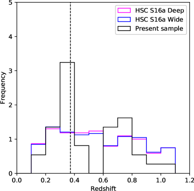
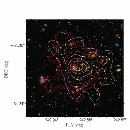
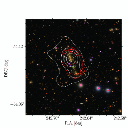
The CAMIRA catalog comprises 2086 clusters at in the S16A Wide and Deep fields (Oguri et al., 2018). We cross-correlated the CAMIRA catalog with the 3XMM-DR7 catalog (Rosen et al., 2016) to find that there are X-ray sources within from the optical centers. We then excluded a XXL survey region overlapped with that of the HSC-SSP survey from the above search result; an X-ray study in the XXL field is to be done through the HSC-XXL external collaboration. To do the systematic X-ray analysis of high-richness clusters, we construct the sample by selecting objects with richness . This richness range corresponds to the cluster mass (Okabe et al., 2018). Therefore, as listed in Table 2, the present sample consists of 37 clusters at , whose distribution is overlaid on that of the CAMIRA clusters with (Figure 1). Except for HSC J141508-002936 at (alternative name is Abell 1882) for which X-ray data were taken by pointed XMM-Newton observations (Miyaoka et al., 2018), X-ray emissions from these clusters are serendipitously detected inside the XMM-Newton fields of view. The average (median) redshift is 0.50 (0.37). Examples of HSC images of the CAMIRA clusters are shown in Figure 2.
Because we require typically more than 1000 cluster-photon counts so as to enable X-ray spectroscopic measurements of the gas temperature and luminosity, the sample is subdivided into two: 17 clusters with cluster-photon counts and 20 clusters with counts111The sum of X-ray counts observed by XMM-Newton EPIC sensors., which are listed in the 1–17th and 18–37th rows of Table 2, respectively. The former (latter) subsample has the average redshift of 0.33 (0.67). The total sample covers the equivalent redshift range of the CAMIRA catalog, but has a lower average redshift. The Kolmogorov-Smirnov (K-S) test gave the probability that the two samples are from the same redshift distribution as (the K-S parameter ), while the K-S test yielded () for the richness distribution. At the 5% significance level, the null hypothesis is not rejected (rejected) in the former (latter) case. We found that the K-S statistics has been improved by including the twenty clusters with low counts, however, the above test suggests that the present measurement is subject to a selection bias. Ideally, a sample of purely optically-selected clusters will be constructed by cross-matching the CAMIRA catalog with the XXL (Pierre et al., 2016b) or future eROSITA cluster catalog, which enables unbiased study of X-ray properties of the optically-selected sample including objects with upper limits where no X-ray emission is detected. This is not possible for the present study, and the selection bias will be examined in section 4.2.
Table 2 lists the location of BCGs identified by the CAMIRA algorithm (Oguri et al., 2018). Note that for 4 out of 37 clusters, the BCGs are clearly misidentified by the CAMIRA algorithm for either one of the following reasons; i) there is another elliptical galaxy near the cluster center brighter than that listed in the CAMIRA catalog, ii) the BCG in the CAMIRA catalog lies outside the X-ray core and there is equivalently bright one inside the core. Since we are interested in physical offsets between BCGs and X-ray peaks rather than miscentering of optical cluster finding algorithms, we correct the BCG coordinates for these four (HSC J140309-001833, HSC J021427-062720, HSC J100049+013820, HSC J222210-004421) by visual inspection of their HSC images.
Sample list. Cluster a BCG position X-ray centroid b c OBSIDd Exposuree (Mpc/\arcsec) RA, Dec (deg) RA, Dec (deg) (kpc) (kpc) M1, M2, PN HSC J142624-012657 0.460 69.7 0.835 / 142 216.6011 , -1.4492 216.5989 , -1.4502 52 23 (23,60) 0674480701 12.3 , 0.6 , 9.1 HSC J021115-034319 0.745 52.3 0.653 / 88 32.8135 , -3.7219 32.8132 , -3.7225 18 60 (60,77) 0655343861 7.7 , 13.0 , 3.4 HSC J095939+023044 0.730 51.7 0.657 / 90 149.9132 , 2.5122 149.9188 , 2.5193 239 196 (190,287) 0203361701 30.1 , 30.2 , 24.3 HSC J161136+541635 0.332 48.3 0.807 / 168 242.8998 , 54.2763 242.8981 , 54.2771 22 38 (38,43) 0059752301 4.9 , 4.7 , 2.9 HSC J090914-001220 0.303 46.5 0.811 / 180 137.3075 , -0.2056 137.3086 , -0.2052 20 23 (22,40) 0725310142 2.5 , 2.7 , 2.4 HSC J141508-002936 0.144 43.0 0.860 / 340 213.7850 , -0.4932 213.7835 , -0.4891 40 50 (39,62) 0145480101 11.0 , 11.8 , 6.9 HSC J140309-001833 0.449 39.7 0.715 / 124 210.7876 , -0.3091 210.7939 , -0.3069 76 36 (15,36) 0606430501 20.4 , 21.1 , 13.3 HSC J095737+023426 0.372 37.4 0.734 / 142 149.4043 , 2.5738 149.4050 , 2.5748 23 14 (14,44) 0203362201 28.9 , 29.0 , 12.3 HSC J022135-062618 0.300 35.7 0.754 / 169 35.3947 , -6.4384 35.4069 , -6.4457 228 10 (10,13) 0655343837 2.6 , 2.6 , 2.2 HSC J232924-004855 0.310 35.2 0.746 / 163 352.3487 , -0.8154 352.3495 , -0.8147 17 44 (44,44) 0673002346 3.5 , 3.8 , 1.8 HSC J022512-062259 0.202 33.0 0.775 / 232 36.3012 , -6.3831 36.2985 , -6.3811 40 246 (246,262) 0655343836 2.6 , 2.5 , 2.2 HSC J021427-062720 0.246 31.3 0.746 / 192 33.6071 , -6.4607 33.6186 , -6.4562 171 15 (13,34) 0655343859 2.5 , 2.7 , 2.0 HSC J161039+540554 0.330 29.5 0.702 / 147 242.6626 , 54.0983 242.6697 , 54.1031 109 144 (144,162) 0059752301 4.9 , 4.8 , 2.9 HSC J095903+025545 0.332 26.4 0.679 / 142 149.7614 , 2.9291 149.7620 , 2.9214 133 8 (8,32) 0203361601 19.1 , 0.0 , 8.6 HSC J100049+013820 0.228 23.2 0.692 / 189 150.1898 , 1.6573 150.1923 , 1.6592 41 94 (87,102) 0302351001 37.6 , 38.9 , 28.0 HSC J090743+013330 0.172 23.1 0.711 / 242 136.9295 , 1.5583 136.9540 , 1.5564 260 14 (14,14) 0725310156 2.6 , 2.7 , 2.4 HSC J095824+024916 0.341 20.1 0.625 / 128 149.6001 , 2.8212 149.6001 , 2.8214 5 9 (9,13) 0203362101 59.4 , 59.5 , 51.1 HSC J090754+005732 0.692 43.5 0.639 / 89 136.9765 , 0.9590 136.9769 , 0.9632 111 131 (131,167) 0725310159 2.7 , 2.7 , 2.2 HSC J090541+013226 0.666 39.1 0.629 / 89 136.4217 , 1.5406 136.4213 , 1.5378 74 52 (52,86) 0725310131 8.5 , 8.3 , 7.6 HSC J232924-004855 0.310 35.2 0.746 / 163 352.3487 , -0.8154 352.3487 , -0.8086 113 31 (10,31) 0673002345 2.1 , 3.4 , 0.6 HSC J222210-004421 0.956 32.6 0.505 / 63 335.5444 , -0.7623 335.5386 , -0.7592 188 289 (211,493) 0670020201 4.2 , 4.0 , 2.3 HSC J100221+032807 1.088 31.8 0.466 / 56 150.5864 , 3.4687 150.5873 , 3.4654 102 363 (311,363) 0743110701 0.0 , 29.7 , 24.3 HSC J221211-000821 0.350 30.5 0.701 / 141 333.0477 , -0.1391 333.0477 , -0.1381 17 75 (51,75) 0655346840 0.0 , 2.8 , 2.6 HSC J160424+430438 0.856 30.4 0.525 / 68 241.1001 , 43.0771 241.0993 , 43.0778 26 42 (42,42) 0025740401 12.2 , 12.4 , 6.1 HSC J100300+013152 0.676 30.3 0.582 / 82 150.7505 , 1.5310 150.7484 , 1.5340 93 80 (47,80) 0203360501 26.8 , 0.0 , 18.8 HSC J142203-000402 0.630 30.1 0.597 / 87 215.5124 , -0.0672 215.5195 , -0.0647 187 352 (339,352) 0651740801 0.0 , 7.2 , 4.0 HSC J090419+020641 0.783 29.9 0.545 / 72 136.0793 , 2.1114 136.0797 , 2.1125 30 29 (17,293) 0725310152 2.7 , 0.0 , 2.3 HSC J220625+013905 0.281 27.4 0.706 / 165 331.6036 , 1.6514 331.6068 , 1.6591 129 15 (15,17) 0655346835 2.8 , 3.0 , 0.9 HSC J221422+004706 0.308 26.5 0.689 / 151 333.5930 , 0.7850 333.5857 , 0.7879 129 37 (37,47) 0655346839 3.0 , 3.1 , 2.6 HSC J090806+011956 0.672 26.0 0.558 / 79 137.0261 , 1.3321 137.0190 , 1.3238 279 243 (205,243) 0725310157 0.8 , 0.0 , 3.9 HSC J090509+012428 0.704 26.0 0.548 / 76 136.2884 , 1.4079 136.2908 , 1.4083 64 129 (99,165) 0725310131 8.5 , 8.3 , 7.6 HSC J022246-061703 0.772 24.3 0.517 / 69 35.6923 , -6.2842 35.6894 , -6.2779 189 211 (211,211) 0655343837 2.6 , 2.6 , 2.2 HSC J222121-004630 0.337 23.3 0.654 / 135 335.3380 , -0.7751 335.3446 , -0.7715 131 167 (148,167) 0670020201 4.2 , 4.0 , 2.3 HSC J221726-001020 0.325 21.8 0.645 / 136 334.3594 , -0.1724 334.3585 , -0.1726 15 171 (171,193) 0673000144 4.2 , 3.9 , 3.6 HSC J090602+011443 0.790 21.3 0.493 / 65 136.5097 , 1.2452 136.5127 , 1.2518 196 183 (183,220) 0725310149 0.0 , 2.4 , 1.9 HSC J221538+004227 0.441 20.7 0.597 / 104 333.9099 , 0.7074 333.9049 , 0.7137 166 77 (77,91) 0673000135 4.1 , 4.1 , 3.7 HSC J141648+521039 0.809 20.3 0.480 / 63 214.2018 , 52.1776 214.2007 , 52.1805 82 263 (191,263) 0127921001 49.0 , 48.9 , 0.0 {tabnote} The sample is subdivided to 17 clusters with cluster-photon counts (1–17 rows) and 20 clusters with counts (18–37 rows). a Richness. bCentroid offset (see section 3.2 for definition). cPeak offset (see section 4.1 for definition). The error range estimated by changing the smoothing scale of X-ray image is indicated in the parenthesis (see text). dThe XMM-Newton observation id. e The XMM-Newton EPIC-MOS1(M1), MOS2(M2), and PN exposure time after data filtering (ksec).
3 Analysis
3.1 Data reduction
Observation data files were retrieved from the XMM-Newton Science Archive222http://nxsa.esac.esa.int and reprocessed with the XMM-Newton Science Analysis System v15.0.0 and the Current Calibration Files. The data reduction, including flare screening, point source detection, and estimation of the quiescent particle background, was done in the standard manner by using the XMM Extended Source Analysis Software [ESAS; Snowden et al. (2008); see also Miyaoka et al. (2018)]. In the following analysis, the detected point sources were excluded from the EPIC data.
3.2 Centroid determination
The X-ray centroid of each cluster was determined from the mean of the photon distribution in an aperture circle of radius . This analysis used the 0.4–2.3 keV EPIC composite image (one image pixel is 5\arcsec). Here, was calculated by substituting in Table 2 in the relation, which was deduced from the relation (Arnaud et al., 2005) and the relation (Oguri et al., 2018). Starting with the optical center, we iterated the centroid search until its position converged within 5\arcsec. If contaminating point sources remained in the circle, we excluded the region centered at the sources and their symmetric positions with respect to the centroid determined by the previous iteration so as not to affect the centroid determination (Ota & Mitsuda, 2004). The result is listed in Table 2. The offset between X-ray centroid and BCG position is presented in section 4.1.
3.3 Spectral analysis
To evaluate the gas temperature and bolometric luminosity, we derive the X-ray spectra by extracting the EPIC data from a circular region within a radius of centered on the X-ray centroid. For 17 clusters with sufficient photon statistics, the spectra were rebinned so that each spectral bin contains over 25 counts. After subtracting the quiescent particle background, the observed spectra of the EPIC MOS/PN cameras in the 0.3–10/0.4–10 keV band were simultaneously fit by using XSPEC 12.9.1 (Arnaud, 1996).
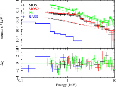
The spectral model consists of (i) cluster thermal emission and (ii) background components. For (i), we used the APEC thin-thermal plasma model version 3.0.8 (Smith et al., 2001; Foster et al., 2012) with the Galactic photoelectric absorption model phabs (Balucinska-Church & McCammon, 1992). The cluster redshift and metal abundance were fixed at the optical value [Table 2; Oguri et al. (2018)] and at 0.3 solar, respectively. The Galactic hydrogen column density was fixed at a value taken from the Leiden/Argentine/Bonn survey (Kalberla et al., 2005). For (ii), the Galactic emission and the cosmic X-ray background were evaluated by jointly fitting the RASS spectra (Snowden et al., 1997) taken from the ring region around the cluster. The other components due to possible solar wind charge exchange, soft proton events, and instrumental fluorescent lines were determined by adding a power-law model and narrow Gaussian lines to the model. An example of the spectral fitting is shown in Figure 3. The resultant APEC model parameters are summarized in Table 3.3. The bolometric luminosity was estimated from the best-fit model flux in the source-frame energy range of 0.01 – 30 keV. The missing flux due to the point-source removal was corrected by interpolating the ICM emission assuming that the observed cluster brightness profile is approximated by the -model (Cavaliere & Fusco-Femiano, 1976).
The XMM + RASS joint fitting gives a reasonable result for most of clusters; however, the background subtraction is not perfect at high energies, particularly for the three clusters, HSC J021115-034319, HSC J021427-062720, and HSC J161039+540554. This is likely to be due to the residual soft proton flares, as indicated by the count-rate ratio between in-FOV and out-FOV (De Luca & Molendi, 2004). The EPIC-MOS1 (MOS2) count-rate ratio (in-FOV)/(out-FOV) is 2.7 (2.2), 1.1 (1.2), 1.4 (1.4) for HSC J021115-034319, HSC J021427-062720, and HSC J161039+540554, respectively. Thus, to check the background uncertainty, we subtract the local background extracted from an annulus centered on the X-ray centroid and fit the APEC model to the observed spectra. Since the resultant parameters are consistent with those obtained from the XMM + RASS joint analysis within that statistics for 14 clusters, we quote the values obtained from the analysis by using the local background for the three clusters mentioned above (see Table 3.3).
For 20 clusters with low counts, we convert the observed cluster counts to bolometric luminosity assuming the APEC model with temperature inferred by the relation (Oguri et al., 2018). The background was estimated from an annulus centered on the X-ray centroid. We checked the robustness of this method by applying the same procedure to 17 clusters with higher counts. In most of them, the luminosity agrees with the result of spectral analysis within the statistical errors, while several clusters have a larger uncertainty up to a factor of . Therefore, for 20 clusters, we take into account the upper limit on the luminosity when we fit the relation (section 4.2).
Results of spectral analysis under APEC thermal plasma model. Cluster /d.o.f. () (keV) () HSCJ142624-012657 3.21 71.3 / 63 HSCJ021115-034319 1.95 95.3 / 81 HSCJ095939+023044 1.71 105.5 / 108 HSCJ161136+541635 0.95 73.8 / 69 HSCJ090914-001220 2.73 48.4 / 33 HSCJ141508-002936 3.27 471.1 / 404 HSCJ140309-001833 3.66 114.4 / 122 HSCJ095737+023426 1.85 153.6 / 154 HSCJ022135-062618 2.73 23.9 / 13 HSCJ232924-004855 4.33 60.7 / 38 HSCJ022512-062259 2.95 78.8 / 71 HSCJ021427-062720 2.13 62.7 / 62 HSCJ161039+540554 0.94 45.6 / 43 HSCJ095903+025545 1.79 126.7 / 160 HSCJ100049+013820 1.80 114.9 / 119 HSCJ090743+013330 3.20 31.0 / 22 HSCJ095824+024916 1.84 314.9 / 280 HSCJ090754+005732 3.04 3.6 HSCJ090541+013226 3.51 3.4 HSCJ232924-004855 4.33 3.3 HSCJ222210-004421 4.72 3.3 HSCJ100221+032807 1.66 3.1 HSCJ221211-000821 4.40 3.1 HSCJ160424+430438 1.09 3.0 HSCJ100300+013152 2.07 3.0 HSCJ142203-000402 2.86 3.0 HSCJ090419+020641 3.66 3.0 HSCJ220625+013905 4.17 3.0 HSCJ221422+004706 3.50 2.9 HSCJ090806+011956 3.12 2.8 HSCJ090509+012428 3.59 2.8 HSCJ022246-061703 2.78 2.8 HSCJ222121-004630 4.73 2.7 HSCJ221726-001020 4.78 2.7 HSCJ090602+011443 3.44 2.6 HSCJ221538+004227 3.71 2.5 HSCJ141648+521039 1.07 2.5 {tabnote} a The gas temperature in keV. For 17 high-count clusters, was derived from spectral fitting. For 20 low-counts cluters, was estimated from richness and the relation. b The bolometric luminosity within the scale radius
4 Results
4.1 Centroid offset and peak offset
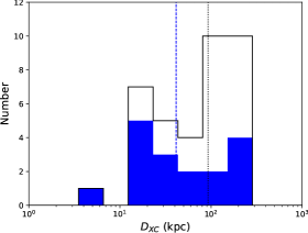
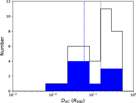
We define the centroid offset as a projected distance between the BCG coordinates and the X-ray centroid measured within . The measured centroid offset is given in Table 2. The histograms of the centroid offset in kpc and fractions of are shown in the upper panels of Figure 4. The median values of centroid offset are given in Table 4.1, which is kpc or for 17 clusters and kpc or for the entire sample.
Median values of centroid offset and peak offset. Fractiona (kpc) () (kpc) () 17 clusters 41 0.06 36 0.05 % 20 clusters 112 0.18 130 0.22 % All 92 0.16 56 0.29 % {tabnote} a Fraction of relaxed clusters and the statistical (systematic) errors (see text).
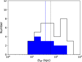
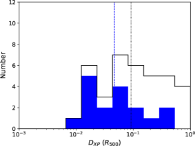
Next, we measured the X-ray peak position within by using the XMM composite image smoothed with a (pixels) Gaussian function. We define the peak offset as a projected distance relative to the BCG coordinates. The resultant peak offset is shown in Table 2 and the median values are given in Table 4.1. The lower panels of Figure 4 show the histograms of the measured peak offset in units of kpc and . For 17 clusters, the median is kpc or . For the entire sample, kpc or .
The twenty clusters with low statistics tend to show larger centroid and peak offsets. As discussed in Mann & Ebeling (2012), the accuracy of the X-ray peak position depends on the statistical quality of the X-ray observations as well as the surface brightness distribution, which varies significantly between clusters. We assessed the standard error of the peak offset by comparing X-ray images of each cluster with different smoothing scale ( pixels). For 17 clusters, ranges from 3% to 68% (the mean is 24%). On the other hand, the entire sample contains objects with larger uncertainties, resulting (the mean is 22%).
We divide the sample into two classes, “relaxed” clusters with a small peak offset () and “disturbed” clusters with a large offset () following the criteria used in Sanderson et al. (2009). As a result, there are only 5 relaxed clusters and the fraction of relaxed objects is for the entire sample, and % if 20 clusters with low photon statistics are excluded. Here the first error is the statistical uncertainty estimated by the bootstrap resampling method (Efron, 1982) and second error in the parenthesis indicates the systematic uncertainty in the measurement and was estimated by referring to the peak-to-peak amplitude of the relaxed fraction in the case that we varied the smoothing scale of the X-ray images between 2 and 4 pixels. Section 5.1 compares the fraction of relaxed clusters in the optical clusters with nearby X-ray and SZE cluster samples.
4.2 Luminosity-temperature relation
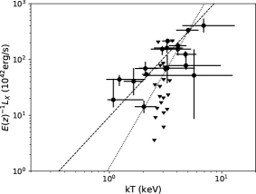
In the self-similar model, the redshift evolution of the cluster scaling relations is described by the factor and the luminosity of the cluster gas in the hydrostatic state follows . Within this framework, the normalization of the luminosity-temperature relation evolves as (Giles et al., 2016). Despite a number of observational studies, however, no clear consensus has been reached on the evolution of the scaling relations (for a review, see Giodini et al., 2013). In the present paper, we correct the redshift evolution by applying the self-similar model and plot against gas temperature in the left panel of Figure 5.
We fit the observed relation to the power-law model (equation 1). To account for measurement errors in both variables, we use the Bayesian regression method (Kelly, 2007) because it has been demonstrated that it outperforms other common estimators that can constrain the parameters even when data have large measurement errors or only upper limits. The quantities , , and the intrinsic scatter are treated as free parameters.
| (1) |
For 17 clusters, the best-fit parameters are , , and . For the entire sample, the uncertainties become larger; , , and , however, they are consistent within the statistical errors.
For comparison, if we apply the BCES code (Akritas & Bershady, 1996) to the present optical sample, the fitting yields the best-fit slope steeper than 2.0 but with a fairly large uncertainty; namely, . Kelly (2007) noted that the BCES estimate of the slope tends to suffer some bias and becomes considerably unstable when the measurement errors are large and/or the sample size is small. Therefore, in section 5.2 we quote the above results based on the Bayesian regression method.
Since the present sample was selected by cross-matching the optical clusters with the X-ray catalog and their exposures available in the XMM-Newton archive is not homogeneous, we study the impact of selection effect on the scaling relation as follows: i) 37 clusters are randomly chosen out of the CAMIRA catalog, ii) the X-ray temperature and luminosity are estimated from the richness assuming the best-fit and relations and the intrinsic scatters, and the errors are assigned. Here only upper limit on luminosity is given to 12 clusters to mimic the actual observations (Table 3.3). iii) the relation was fit to determine the coefficients in equation 1. iv) steps i)–iii) are repeated times. From the resultant parameter distributions, we find that () tends to be underestimated (overestimated) by (). A similar trend was seen if we limit the sample to 17 clusters with better statistics. We thus regard the above quantities as systematic errors of the relation caused by the selection effect and compare our results with previous studies in section 5.2.
5 Discussion
Our analyses of two sub-samples yielded consistent results within measurement uncertainties. Due to the shallow exposures of 20 clusters, however, we will discuss interpretations of the present results primarily based on the observations of 17 clusters with higher counts.
5.1 Centroid offset and the cluster dynamical state
In section 4.1 we quantified the centroid offset and peak offset from the XMM image analysis to find that half of the sample has the centroid (peak) offset larger than () or 41 kpc (36 kpc). Following the criteria used in Sanderson et al. (2009), Rossetti et al. (2016) estimated the fraction of relaxed clusters in the Planck SZE sample to be %. They also calculated the fraction to be % in X-ray selected cluster samples constructed from the HIFLUGCS, MACS, and REXCESS surveys, whereas we obtain only % from our optical sample. This suggests that the optical cluster sample contains a larger fraction of disturbed clusters particularly in comparison with the X-ray selected cluster samples.
X-ray observations preferentially detect relaxed clusters having cool cores at the center as opposed to more disturbed, non-cool-core clusters found in SZE surveys (Eckert et al., 2011; Rossetti et al., 2017; Andrade-Santos et al., 2017; Lovisari et al., 2017). Andreon et al. (2016) found a wider population in the sample selected independently of X-ray properties than seen in the SZE surveys. Furthermore, Chon & Böhringer (2017) claim that the cool-core bias in previous X-ray surveys is due to the survey-selection method such as for a flux-limited survey, and is not due to the inherent nature of X-ray selection. Therefore, considering the nature of the HSC cluster survey, we suggest that the observed small fraction of relaxed clusters in the present optical sample is due to the fact that the CAMIRA algorithm is immune to the dynamical state of X-ray-emitting gas and is likely to detect clusters with a wider range of cluster morphology. This needs to be confirmed with the large uniform sample to be constructed by the eROSITA survey.
Given a higher merger rate in the distant universe, the redshift evolution of X-ray morphology is likely to affect the measurement of the fraction of relaxed clusters with respect to disturbed clusters. Mann & Ebeling (2012) reported based on the Chandra observations that the fraction of morphologically-disturbed clusters increases at for the X-ray luminous clusters. On the other hand, McDonald et al. (2017) found that there is no measurable redshift evolution in the X-ray morphology of massive clusters. In our optical cluster sample, the redshift evolution is not significantly seen; the fractions of relaxed clusters estimated from the X-ray peak offsets are % at and % at .
5.2 Scaling relations
We obtained the slope of of the relation for the present optical clusters. Note that the second error in the parenthesis indicates the systematic uncertainty due to the sample selection (section 4.2). This is consistent with the slope of 2.0 predicted from the self-similar model, whereas a steeper slope of has been reported by many X-ray observations in the past (for review, see Giodini et al., 2013). Even so, the data points lie within the observed large scatter of X-ray clusters on the plane (Takey et al., 2011).
The gas density in the core region is known to have a significant scatter, and the self-similar relation is not satisfied particularly in clusters with a compact, cooling core (e.g., Ota et al., 2006). In the present sample, the fraction of relaxed cluster is % (section 4.1) and our preliminary analysis of the X-ray brightness profile shows that there are only a few objects that have a very small core radius ( kpc), suggesting that the impact of cool core on the relation is likely to be small.
The fitted slope agrees with that of the Red-sequence Cluster Survey at high redshifts [the slope parameter is ; Hicks et al. (2008)] and that of the total RCS sample; namely, 18 clusters at [; Hicks et al. (2013)] within the errors. In comparison with X-ray selected samples that contain a large number of clusters () at a wide redshift range [; Reichert et al. (2011), ; Takey et al. (2011), ; Maughan et al. (2012)], the present sample shows a marginally shallower slope. To further confirm the result, however, we need to increase the number of clusters and improve the accuracy with which the relation is measured.
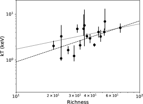
The right panel of Figure 5 shows the relationship between gas temperature and optical richness. Although the scatter is large, the positive correlation is seen and the correlation coefficient is calculated to be 0.58. Assuming the power-law model,
| (2) |
the fit to the data yields and . This is marginally steeper than the best-fit power-law relation derived for 50 bright X-ray clusters in the XXL and XXL-LSS fields [, ; Oguri et al. (2018)]. Because the gas temperature of XXL and XXL-LSS clusters was measured in the central kpc region (Pierre et al., 2004, 2016b), direct comparison is not easy. Conversely, the self-similar model predicts given that the cluster mass is related to richness and temperature through and , respectively. Thus our fitting result is consistent with the self-similar model, although the statistical uncertainty is large. Recently, Okabe et al. (2018) reported based on the weak-lensing analysis of 1750 clusters in the CAMIRA catalog (Oguri et al., 2018) that the relation has a stepper slope of . This modifies the above expectation from to , which is, however, consistent with our result within the error.
6 Summary and future prospects
Using the XMM-Newton archive data, we apply an X-ray analysis to 37 rich, optical clusters of galaxies at in the HSC-SSP field. Most of the clusters were serendipitously detected in the XMM-Newton fields of view. We subdivided the sample to two, i.e., 17 (20) clusters with high (low) photon counts, to find the results of two subsamples agree with each other within errors. Due to large statistical uncertainties in the 20 clusters, however, we discussed the implications mainly based on the results for 17 clusters with sufficient statistics. The major findings are as follows:
-
1.
We systematically analyzed the X-ray centroid or peak offset as compared with the BCG position. The fraction of relaxed clusters in the optical cluster sample, which is defined based on the offset between the BCG and X-ray peak, is %. This is less than that of the X-ray samples. Because the optical sample is immune to the cool-core bias, it is likely to contain more disturbed clusters and thus cover a larger range of the cluster morphology.
-
2.
The slope of the luminosity-temperature relation is marginally less than that of X-ray samples and is consistent with the self-similar model prediction of 2.0. The slope of the temperature-richness relation is also consistent with the prediction of the self-similar model although the former has a large statistical uncertainty.
Our pilot study provides important information about the X-ray properties of the optical clusters, which are marginally different from those observed in the X-ray samples. To obtain more conclusive results, we need to improve the measurement accuracy and the sample uniformity. We thus plan to extend the analysis by (1) incorporating fainter objects in the 3MM-DR7 catalog and (2) conducting X-ray observations of the massive, high-redshift () clusters newly discovered by the HSC-SSP survey. For the latter, the XMM-Newton follow-up project is now ongoing and is to be the subject of an upcoming presentation. Furthermore, by the time of completion of the HSC-SSP survey, the CAMIRA cluster catalog will be about 6-times larger than that at present. These works should allow us to derive the mass-observable scaling by using a larger number of clusters and study the redshift evolution of the X-ray properties of the optical clusters. Detailed comparisons of optical, weak lensing, SZE, and X-ray selected clusters will improve our knowledge of cluster-mass calibration and cluster evolution.
The Hyper Suprime-Cam (HSC) collaboration includes the astronomical communities of Japan and Taiwan, and Princeton University. The HSC instrumentation and software were developed by the National Astronomical Observatory of Japan (NAOJ), the Kavli Institute for the Physics and Mathematics of the Universe (Kavli IPMU), the University of Tokyo, the High Energy Accelerator Research Organization (KEK), the Academia Sinica Institute for Astronomy and Astrophysics in Taiwan (ASIAA), and Princeton University. Funding was contributed by the FIRST program from Japanese Cabinet Office, the Ministry of Education, Culture, Sports, Science and Technology (MEXT), the Japan Society for the Promotion of Science (JSPS), Japan Science and Technology Agency (JST), the Toray Science Foundation, NAOJ, Kavli IPMU, KEK, ASIAA, and Princeton University.
This paper makes use of software developed for the Large Synoptic Survey Telescope. We thank the LSST Project for making their code available as free software at http://dm.lsst.org
The Pan-STARRS1 Surveys (PS1) have been made possible through contributions of the Institute for Astronomy, the University of Hawaii, the Pan-STARRS Project Office, the Max-Planck Society and its participating institutes, the Max Planck Institute for Astronomy, Heidelberg and the Max Planck Institute for Extraterrestrial Physics, Garching, The Johns Hopkins University, Durham University, the University of Edinburgh, Queen’s University Belfast, the Harvard-Smithsonian Center for Astrophysics, the Las Cumbres Observatory Global Telescope Network Incorporated, the National Central University of Taiwan, the Space Telescope Science Institute, the National Aeronautics and Space Administration under Grant No. NNX08AR22G issued through the Planetary Science Division of the NASA Science Mission Directorate, the National Science Foundation under Grant No. AST-1238877, the University of Maryland, and Eotvos Lorand University (ELTE) and the Los Alamos National Laboratory.
We are grateful to Chien-Hsiu Lee for useful comments. This work was supported in part by JSPS KAKENHI grants 16K05295 (NO) and JP15K17610 (SU). YI is supported by Rikkyo University Special Fund for Research (SFR). This work is supported in part by the Ministry of Science and Technology of Taiwan (grant MOST 106-2628-M-001-003-MY3) and by Academia Sinica (grant AS-IA-107-M01). We thank the anonymous referee for useful suggestions.
References
- Aihara et al. (2018a) Aihara, H., Armstrong, R., Bickerton, S., et al. 2018a, PASJ, 70, S8
- Aihara et al. (2018b) Aihara, H., Arimoto, N., Armstrong, R., et al. 2018b, PASJ, 70, S4
- Akritas & Bershady (1996) Akritas, M. G., & Bershady, M. A. 1996, ApJ, 470, 706
- Allen et al. (2011) Allen, S. W., Evrard, A. E., & Mantz, A. B. 2011, ARA&A, 49, 409
- Andrade-Santos et al. (2017) Andrade-Santos, F., Jones, C., Forman, W. R., et al. 2017, ApJ, 843, 76
- Andreon et al. (2016) Andreon, S., Serra, A. L., Moretti, A., & Trinchieri, G. 2016, A&A, 585, A147
- Arnaud (1996) Arnaud, K. A. 1996, in Astronomical Society of the Pacific Conference Series, Vol. 101, Astronomical Data Analysis Software and Systems V, ed. G. H. Jacoby & J. Barnes, 17
- Arnaud et al. (2005) Arnaud, M., Pointecouteau, E., & Pratt, G. W. 2005, A&A, 441, 893
- Balucinska-Church & McCammon (1992) Balucinska-Church, M., & McCammon, D. 1992, ApJ, 400, 699
- Bleem et al. (2015) Bleem, L. E., Stalder, B., de Haan, T., et al. 2015, ApJS, 216, 27
- Böhringer et al. (2001) Böhringer, H., Schuecker, P., Guzzo, L., et al. 2001, A&A, 369, 826
- Bosch et al. (2018) Bosch, J., Armstrong, R., Bickerton, S., et al. 2018, PASJ, 70, S5
- Bulbul et al. (2019) Bulbul, E., Chiu, I.-N., Mohr, J. J., et al. 2019, ApJ, 871, 50
- Cavaliere & Fusco-Femiano (1976) Cavaliere, A., & Fusco-Femiano, R. 1976, A&A, 500, 95
- Chon & Böhringer (2017) Chon, G., & Böhringer, H. 2017, A&A, 606, L4
- De Luca & Molendi (2004) De Luca, A., & Molendi, S. 2004, A&A, 419, 837
- Diemer & Kravtsov (2015) Diemer, B., & Kravtsov, A. V. 2015, ApJ, 799, 108
- Donahue et al. (2014) Donahue, M., Voit, G. M., Mahdavi, A., et al. 2014, ApJ, 794, 136
- Eckert et al. (2011) Eckert, D., Molendi, S., & Paltani, S. 2011, A&A, 526, A79
- Efron (1982) Efron, B. 1982, The Jackknife, the Bootstrap and other resampling plans
- Foster et al. (2012) Foster, A. R., Ji, L., Smith, R. K., & Brickhouse, N. S. 2012, ApJ, 756, 128
- Furusawa et al. (2018) Furusawa, H., Koike, M., Takata, T., et al. 2018, PASJ, 70, S3
- Giles et al. (2016) Giles, P. A., Maughan, B. J., Pacaud, F., et al. 2016, A&A, 592, A3
- Giodini et al. (2013) Giodini, S., Lovisari, L., Pointecouteau, E., et al. 2013, Space Sci. Rev., 177, 247
- Hicks et al. (2008) Hicks, A. K., Ellingson, E., Bautz, M., et al. 2008, ApJ, 680, 1022
- Hicks et al. (2013) Hicks, A. K., Pratt, G. W., Donahue, M., et al. 2013, MNRAS, 431, 2542
- Hilton et al. (2017) Hilton, M., Hasselfield, M., Sifón, C., et al. 2017, ArXiv e-prints
- Hoekstra et al. (2015) Hoekstra, H., Herbonnet, R., Muzzin, A., et al. 2015, MNRAS, 449, 685
- Kalberla et al. (2005) Kalberla, P. M. W., Burton, W. B., Hartmann, D., et al. 2005, A&A, 440, 775
- Katayama et al. (2003) Katayama, H., Hayashida, K., Takahara, F., & Fujita, Y. 2003, ApJ, 585, 687
- Kawanomoto et al. (2018) Kawanomoto, S., Uraguchi, F., Komiyama, Y., et al. 2018, in prep.
- Kelly (2007) Kelly, B. C. 2007, ApJ, 665, 1489
- Komiyama et al. (2018) Komiyama, Y., Obuchi, Y., Nakaya, H., et al. 2018, PASJ, 70, S2
- Lodders & Palme (2009) Lodders, K., & Palme, H. 2009, Meteoritics and Planetary Science Supplement, 72, 5154
- Lovisari et al. (2017) Lovisari, L., Forman, W. R., Jones, C., et al. 2017, ApJ, 846, 51
- Mahdavi et al. (2013) Mahdavi, A., Hoekstra, H., Babul, A., et al. 2013, ApJ, 767, 116
- Mann & Ebeling (2012) Mann, A. W., & Ebeling, H. 2012, MNRAS, 420, 2120
- Mantz et al. (2016) Mantz, A. B., Allen, S. W., Morris, R. G., et al. 2016, MNRAS, 463, 3582
- Martino et al. (2014) Martino, R., Mazzotta, P., Bourdin, H., et al. 2014, MNRAS, 443, 2342
- Maughan et al. (2012) Maughan, B. J., Giles, P. A., Randall, S. W., Jones, C., & Forman, W. R. 2012, MNRAS, 421, 1583
- McDonald et al. (2017) McDonald, M., Allen, S. W., Bayliss, M., et al. 2017, ApJ, 843, 28
- Merloni et al. (2012) Merloni, A., Predehl, P., Becker, W., et al. 2012, ArXiv e-prints
- Miyaoka et al. (2018) Miyaoka, K., Okabe, N., Kitaguchi, T., et al. 2018, PASJ, 70, S22
- Miyazaki et al. (2012) Miyazaki, S., Komiyama, Y., Nakaya, H., et al. 2012, in Proc. SPIE, Vol. 8446, Ground-based and Airborne Instrumentation for Astronomy IV, 84460Z
- Miyazaki et al. (2015) Miyazaki, S., Oguri, M., Hamana, T., et al. 2015, ApJ, 807, 22
- Miyazaki et al. (2018) Miyazaki, S., Komiyama, Y., Kawanomoto, S., et al. 2018, PASJ, 70, S1
- Oguri (2014) Oguri, M. 2014, MNRAS, 444, 147
- Oguri et al. (2018) Oguri, M., Lin, Y.-T., Lin, S.-C., et al. 2018, PASJ, 70, S20
- Okabe et al. (2014) Okabe, N., Umetsu, K., Tamura, T., et al. 2014, PASJ, 66, 99
- Okabe et al. (2018) Okabe, N., Oguri, M., Akamatsu, H., et al. 2018, arXiv e-prints
- Ota et al. (2006) Ota, N., Kitayama, T., Masai, K., & Mitsuda, K. 2006, ApJ, 640, 673
- Ota & Mitsuda (2004) Ota, N., & Mitsuda, K. 2004, A&A, 428, 757
- Pierre et al. (2004) Pierre, M., Valtchanov, I., Altieri, B., et al. 2004, J. Cosmology Astropart. Phys, 9, 011
- Pierre et al. (2016a) Pierre, M., Pacaud, F., Adami, C., et al. 2016a, A&A, 592, A1
- Pierre et al. (2016b) —. 2016b, A&A, 592, A1
- Reichert et al. (2011) Reichert, A., Böhringer, H., Fassbender, R., & Mühlegger, M. 2011, A&A, 535, A4
- Rosen et al. (2016) Rosen, S. R., Webb, N. A., Watson, M. G., et al. 2016, A&A, 590, A1
- Rossetti et al. (2017) Rossetti, M., Gastaldello, F., Eckert, D., et al. 2017, MNRAS, 468, 1917
- Rossetti et al. (2016) Rossetti, M., Gastaldello, F., Ferioli, G., et al. 2016, MNRAS, 457, 4515
- Rozo & Rykoff (2014) Rozo, E., & Rykoff, E. S. 2014, ApJ, 783, 80
- Rykoff et al. (2014) Rykoff, E. S., Rozo, E., Busha, M. T., et al. 2014, ApJ, 785, 104
- Rykoff et al. (2016) Rykoff, E. S., Rozo, E., Hollowood, D., et al. 2016, ApJS, 224, 1
- Sanders et al. (2018) Sanders, J. S., Fabian, A. C., Russell, H. R., & Walker, S. A. 2018, MNRAS, 474, 1065
- Sanderson et al. (2009) Sanderson, A. J. R., Edge, A. C., & Smith, G. P. 2009, MNRAS, 398, 1698
- Smith et al. (2016) Smith, G. P., Mazzotta, P., Okabe, N., et al. 2016, MNRAS, 456, L74
- Smith et al. (2001) Smith, R. K., Brickhouse, N. S., Liedahl, D. A., & Raymond, J. C. 2001, ApJ, 556, L91
- Snowden et al. (2008) Snowden, S. L., Mushotzky, R. F., Kuntz, K. D., & Davis, D. S. 2008, A&A, 478, 615
- Snowden et al. (1997) Snowden, S. L., Egger, R., Freyberg, M. J., et al. 1997, ApJ, 485, 125
- Sun et al. (2009) Sun, M., Voit, G. M., Donahue, M., et al. 2009, ApJ, 693, 1142
- Takey et al. (2011) Takey, A., Schwope, A., & Lamer, G. 2011, A&A, 534, A120
- Takey et al. (2013) —. 2013, A&A, 558, A75
- Tanaka et al. (2018) Tanaka, M., Coupon, J., Hsieh, B.-C., et al. 2018, PASJ, 70, S9
- Vikhlinin et al. (2006) Vikhlinin, A., Kravtsov, A., Forman, W., et al. 2006, ApJ, 640, 691
- von der Linden et al. (2014) von der Linden, A., Mantz, A., Allen, S. W., et al. 2014, MNRAS, 443, 1973
- Zhang et al. (2008) Zhang, Y.-Y., Finoguenov, A., Böhringer, H., et al. 2008, A&A, 482, 451