Critical behavior in 3-d gravitational collapse of massless scalar fields
Abstract
We present results from a study of critical behavior in 3-d gravitational collapse with no symmetry assumptions. The source of the gravitational field is a massless scalar field. This is a well-studied case for spherically symmetric gravitational collapse, allowing us to understand the reliability and accuracy of the simulations. We study both supercritical and subcritical evolutions to see if one provides more accurate results than the other. We find that even for non-spherical initial data with 35 percent of the power in the spherical harmonic, the critical solution is the same as in spherical symmetry.
I Introduction
Critical behavior in the gravitational collapse of a massless scalar field was discovered by Choptuik Choptuik (1993), who sought to answer the question “What happens at the threshold of black hole formation?” Choptuik considered a massless scalar field undergoing gravitational collapse in a spherically symmetric spacetime. He found that for some parameter in the initial data, for example the amplitude of a Gaussian-distributed scalar field, the final mass of the black hole is related to by
| (1) |
Here is the critical value of the parameter that separates initial data that form a black hole (supercritical) from initial data that do not form a black hole (subcritical). Choptuik observed that the critical exponent is independent of the initial data chosen—the critical behavior is universal. The currently accepted value of the critical exponent is Gundlach (1997a). Not much later, Garfinkle and Duncan Garfinkle and Duncan (1998) discovered that in subcritical evolutions the maximum absolute value of the Ricci scalar at the center of the collapse obeys the scaling relation
| (2) |
Interestingly, was found to have the same value as .
Another key aspect of the critical behavior observed by Choptuik is that of a discretely self-similar solution, or “echoing”. In the strong-field regime near the critical solution, Choptuik noticed that any gauge-invariant quantity obeys the relation
| (3) |
where is a dimensionless constant. Here , where is the proper time of a central observer and is the value of when a naked singularity forms in the limit . is referred to as the accumulation time. As one moves closer in time to the critical solution by , the same field profile is observed for but at spatial scales smaller. The echoing period , like the critical exponent, is universal in the sense that it does not depend on the initial data, only on the type of matter undergoing gravitational collapse. The currently accepted value for a massless scalar field is Gundlach (1997a).
Since the seminal work by Choptuik, many studies to better understand critical behavior in gravitational collapse have been performed. Studies of critical collapse of a massless scalar field in spherical symmetry have found that the critical exponent and echoing period are both independent of the initial data profile but depend on the dimensionality of the spacetime Garfinkle et al. (1999); Bland et al. (2005); Sorkin and Oren (2005); Taves and Kunstatter (2011). Similar studies observed that the critical exponent, echoing period, and possibly even the type of phase transition are changed in modified theories of gravity Deppe et al. (2012); Golod and Piran (2012). Interestingly, the presence of critical behavior appears to be independent of the matter source, but the value of the critical exponent, echoing period, and type of phase transition depend on the type of matter Choptuik et al. (1996); Gundlach (1997b); Brady et al. (1997); Garfinkle et al. (2003); Baumgarte and Montero (2015); Gundlach and Baumgarte (2016); Baumgarte and Gundlach (2016); Gundlach and Baumgarte (2018). Vacuum critical collapse was first studied in Abrahams and Evans (1993, 1994), which found that critical behavior is present and that the critical exponent and echoing period have values different from those found in simulations with matter. Unfortunately, studying vacuum gravitational collapse has proven to be quite difficult Sorkin (2010, 2011); Hilditch et al. (2013, 2016).
In critical collapse the phase transition is either Type I or Type II. In Type II phase transitions the black hole mass continuously goes to zero as is approached. This has been the most common case observed so far when studying critical collapse. In Type I transitions the mass of the black hole that forms approaches a constant, non-zero value as is approached. Type I phase transitions have been clearly identified in critical collapse of a massive scalar fieldBrady et al. (1997). The discussion in this paper is only relevant for Type II critical behavior.
In 1997 both Gundlach Gundlach (1997a), and Hod and Piran Hod and Piran (1997) independently discovered fine structure in addition to the power-law behavior of the black hole masses: There is a small-amplitude modulation of (1). Specifically, the scaling relation is altered to
| (4) |
where , , , and are constants. These authors predicted and verified that for massless scalar field collapse in spherical symmetry. Whether or not this relation holds for different matter sources and beyond spherical symmetry is an open question.
Unfortunately, answering the question of how symmetry assumptions affect the critical exponent and echoing period has turned out to be quite challenging. The reason is that spatiotemporal scales varying over four to six orders of magnitude must be resolved in order to properly study the fine structure and echoing, and a large number of high-resolution simulations are necessary. In addition, the well-posedness and stability of the formulation of the Einstein equations solved and the choice of gauge has proven to be as problematic here as in other simulations in numerical relativity. Akbarian and Choptuik Akbarian and Choptuik (2015) have recently studied how formulations of the Einstein equations commonly used for binary black hole mergers behave when studying critical collapse. However, that work was restricted to spherical symmetry.
Critical collapse of a massless scalar field in axial symmetry was studied using perturbation theory by Martin-Garcia and Gundlach Martin-Garcia and Gundlach (1999), who found that all non-spherical modes decay. In 2003 Choptuik et. al Choptuik et al. (2003) performed numerical simulations of massless scalar field collapse in axial symmetry. They found that the critical solution in this case is the same as the solution found in spherical symmetry. However, in contrast to Martin-Garcia and Gundlach (1999), they also found tentative evidence for a non-decaying mode. More recently, Healy and Laguna Healy and Laguna (2014) studied critical collapse of a massless scalar field that is symmetric about the -plane. Healy and Laguna observed results consist with spherically symmetric collapse, but were unable to verify the echoing of gauge-independent fields. The work of Healy and Laguna has been followed by a study of massless scalar field collapse with a quartic potential by Clough and Lim Clough and Lim (2016). Clough and Lim also studied initial data similar to that of Healy and Laguna (2014) and obtained results similar to those of Healy and Laguna.
In this paper we present a study of critical collapse of a massless scalar field with no symmetry assumptions, and the first study beyond spherical symmetry that is able to resolve the fine structure in the black hole mass scaling relation. We are able to resolve small-scale dynamics in both supercritical and subcritical evolutions, allowing us to directly compare the results. In II we review the equations solved, in III we discuss the initial data used, in IV we provide details about the numerical method, in V we present the results, and we conclude in VI.
II Equations
We study the dynamics near the critical solution in gravitational collapse of the Einstein-Klein-Gordon system. We solve the Einstein equations,
| (5) |
where is the Ricci tensor, the spacetime metric, and the stress tensor. Here and throughout the rest of the paper we will use latin indices at the beginning of the alphabet, e.g. to refer to spacetime indices running from 0 to 3, and later indices, to refer to spatial indices running from 1 to 3. We use the ADM form of the metric,
| (6) |
where is the lapse, the shift, and the spatial metric. We denote the timelike unit normal orthogonal to the spacelike hypersurfaces by
| (7) |
We solve Eq. (5) using a first-order generalized harmonic (GH) formulation Lindblom et al. (2006).
The matter source is a massless scalar field with
| (8) |
To bring the resulting equations of motion into first-order form, we define the auxiliary variables and , and the conjugate variables and .
The first-order GH system is Lindblom et al. (2006)
| (9) | ||||
| (10) | ||||
| (11) |
where is the so-called gauge source function and must satisfy the constraint . The parameters and are described in IV.4. The first-order massless-Klein-Gordon system is
| (12) | ||||
| (13) | ||||
| (14) |
The parameters and are described in IV.4, and is the trace of the extrinsic curvature.
III Initial Data
We generate initial data for the evolutions by solving the extended conformal thin-sandwich equations Pfeiffer and York (2003) using the spectral elliptic solver Pfeiffer et al. (2003) in SpEC SpE . The contributions to the equations from the scalar field are given by
| (15) | ||||
| (16) |
and
| (17) |
where projects the spacetime index onto the spatial hypersurface orthogonal to .
Let and
| (18) |
For concreteness we focus on three types of initial data: spherically symmetric data given by
| (19) |
data where the second term has no -coordinate dependence (recall ) similar to that studied in Healy and Laguna (2014); Clough and Lim (2016)
| (20) |
and finally generic initial data of the form
| (21) |
The conjugate momentum to the in the spherically symmetric case is given by
| (22) |
and is multiplied by the same non-spherical terms as . This is ingoing spherical wave initial data. The numerical factor is chosen so that when , the maximum of the second term is approximately unity. We choose and for the results presented here. For the initial data (20) we (arbitrarily) choose and for data given by (III) we choose .
IV Numerical Methods
IV.1 Domain Decomposition
SpEC decomposes the computational domain into possibly overlapping subdomains. Within each subdomain a suitable set of basis functions that depends on the topology of the subdomain is chosen to approximate the solution. The domain decomposition for finding the initial data is a cube at the center with an overlapping spherical shell that is surrounded by concentric spherical shells. For the evolution, a filled sphere surrounded by non-overlapping spherical shells is used until a black hole forms. At this point a ringdown or excision grid nearly identical to that used during the ringdown phase of binary black hole merger evolutions is used Scheel et al. (2009); Szilagyi et al. (2009); Hemberger et al. (2013). The ringdown grid consists of a set of non-overlapping spherical shells with the inner shell’s inner radius approximately of the apparent horizon radius.
IV.2 Dual Frames and Mesh Refinement
To resolve the large range of spatial and temporal scales required, finite-difference codes typically use adaptive mesh refinement (AMR). However, for the spatiotemporal scales required here, AMR is computationally prohibitively expensive in 3+1 dimensions without any symmetries.
SpEC achieves its high accuracy by using spectral methods to solve the PDEs rather than finite differencing. In addition, two further tools are employed to achieve high accuracy: dual frames Scheel et al. (2006); Szilagyi et al. (2009); Hemberger et al. (2013) and spectral AMR Szilágyi (2014).
In the dual frames approach, the PDEs are solved in what is called the grid frame. This frame is related to the “inertial frame”, the frame in which the PDEs are originally written, by time-dependent spatial coordinate maps. The dual frames method “moves” the grid points inward as the scalar field collapses, which gives an additional two orders of magnitude of resolution compared to the initial inertial coordinates without the use of any mesh refinement. We also employ a coordinate map to slowly drift the outer boundary inward so that any constraint-violating modes near the outer boundary are propagated out of the computational domain. While the slow drift of the outer boundary is not essential for stability, it is helpful in long evolutions.
Denote the coordinate map that moves the grid points inward during collapse by and the map that drifts the outer boundary inward by . Then the coordinate map used during collapse before a black hole forms is given by . The mapping relates the initial coordinates, to the grid coordinates by . The specific spatial coordinate map we use for both and is of the form
| (23) |
where , , is a time-dependent function we call an expansion factor, and is a parameter of the map. For we choose
| (24) |
with , , and . The value of for is . For we use and
| (25) |
with and . We find these choices for the coordinate maps lead to accurate and stable long-term evolutions with sufficient resolution to resolve both scaling and echoing.
After an apparent horizon is found we switch over to an excision grid and use the same coordinate maps used in the ringdown portion of the binary black hole evolutions Scheel et al. (2009); Szilagyi et al. (2009); Hemberger et al. (2013). Specifically, we excise the interior of the apparent horizon with the excision surface’s radius being approximately 94 per cent of the apparent horizon’s coordinate radius. Near the apparent horizon, all the characteristics are directed toward the center of the apparent horizon and so no boundary conditions need to be imposed there. Thus, as long as the excision surface remains close to the apparent horizon, the simulation remains stable without the need to impose additional boundary conditions. One difficulty is that during the very early phase of ringdown the apparent horizon’s coordinate radius increases very rapidly. To deal with the rapid expansion, a control system is used to track the apparent horizon and adjust the location of the excision boundary to follow the apparent horizon Scheel et al. (2006, 2009); Hemberger et al. (2013).
While the spatial coordinate maps work extremely well for resolving the small length scales that appear near the critical solution, they do not provide any guarantees about the truncation error of the simulations. The temporal error is controlled by using an adaptive, fifth-order Dormand-Prince time stepper. The spatial error is controlled using the spectral AMR algorithm described in Szilágyi (2014). Using AMR we control the relative error in the metric, the spatial derivative of the metric and the conjugate momentum of the metric. For the results presented in this manuscript we set a relative maximum spatiotemporal error of .
IV.3 Gauge Choice
In binary black hole evolutions with the GH system, large constraint violations occur unless an appropriate gauge condition is chosen. The key ingredient in a successful choice Lindblom and Szilagyi (2009) is to control the growth of , where is the determinant of the spatial metric. As one might expect, evolutions of critical behavior at black hole formation require even more stringent control of the gauge than in binary simulations. We find that without such control, explosive growth in both and prevents the code from finding an apparent horizon before the constraints blow up and the evolution fails. Accordingly, we adopt a modified version of the damped harmonic gauge used in Ref. Lindblom and Szilagyi (2009):
| (26) |
The coefficients , and are described below.
Fortunately, the region of the spatial hypersurfaces where diverges is different from that where diverges and so having the coefficients and depend on and respectively allows us to control both divergences with a single equation. The functional forms of the coefficients are
| (27) | ||||
| (28) |
and
| (29) |
The roll-on function is given by
| (30) |
where we choose and , while the spatial weight function, is given by
| (31) |
where we set . The function is used to transition from the initial maximal slicing to the damped harmonic gauge needed later in the evolution, while makes the gauge be pure harmonic near the outer boundary of the computational domain. The factors in Eq. (27) and (28) make the gauge pure harmonic in the region of the spatial slice where and are near unity, respectively. We found that using the fourth power as opposed to the second power that is typically used for controlling the growth of in binary black hole evolutions is required for stable long-term evolutions.
IV.4 Constraint Damping
Both the Klein-Gordon and the GH system have constraints that must remain satisfied during evolutions. For the Klein-Gordon system the constraint is
| (32) |
The constraints for the GH system are given in reference Lindblom et al. (2006).
Failure to satisfy the constraints indicates that the numerical simulation is no longer solving the physical system of interest and should not be trusted. To control growth of constraint violations from numerical inaccuracies, constraint damping parameters are added to the evolution equations. For the GH system the constraint damping parameters are and , and for the Klein-Gordon system and . See Eqs.(9–II) for how the constraint damping parameters appear in the evolution equations. We find that choosing and works well for the scalar field. For the GH system, finding good constraint damping parameters is more difficult, especially during ringdown. The dimensions of the constraint damping parameters are , which suggests that for smaller black holes where the characteristic time scale is shorter, the constraint damping parameters must be increased. During ringdown we choose
| (33) | ||||
| (34) | ||||
| (35) |
with , , and . Larger values of and are used for smaller black holes. During the collapse phase of the evolutions we find less sensitivity to the choice of the damping parameters. We use the same functional form as during the ringdown but always choose .
V Results
All files used to produce figures in this paper, including the data, are available from the arXiv version of this paper.
V.1 Scaling
In this section we present two sets of scaling relations. The first involves the final mass of the black hole for supercritical evolutions. For each class of initial data we evolve the data with amplitudes large enough that a black hole forms and gradually decrease the amplitude. While decreasing the amplitude we focus on simulations that form a black hole. Rather than performing a binary search to estimate , we fit the relationship to the data for , , and , where we take to be the amplitude of the initial data. We then use the from the fit to determine an amplitude that should form a black hole but is closer to the critical solution. This is repeated until , the target value. Choosing suitable values of to fit for and is tricky. We describe our procedure in the Appendix. Note that the relationship used for determining which amplitude to use next is not used for analyzing the results.
The second scaling relation involves, the maximum Ricci scalar at the center for subcritical evolutions. We run simulations to obtain an approximately even distribution of masses and maximum Ricci scalars for . We estimate the errors in the final mass of the black hole and using convergence tests with values of nearest .
Once we have reached the target number of simulations, with the lowest amplitude that forms a black hole having , we fit the mass of the resulting black hole to
| (36) |
as suggested in Gundlach (1997a); Hod and Piran (1997). Note that the superscript is not an exponent but denotes that parameter was obtained from fitting to the mass of the black hole rather than the maximum Ricci scalar at the center. We find that the probability of and the reduced are better for this function than the one where the sinusoidal term is omitted. We fit for all parameters in (V.1), including . The fitting function used for the maximum Ricci scalar at the origin is
| (37) |
However, for consistency we use the value of obtained from fitting to the masses when fitting to the maximum Ricci scalar as well.
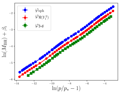
In Fig. 1 we plot as a function of for the three types of initial data studied. For data we arbitrarily choose , which is a large deviation from the spherical solution. For reference, when the scalar field profile is zero at the zeros of . For initial data we choose , an even stronger deviation from spherical symmetry. In Fig. 1 we offset the curves vertically by so that they do not overlap and are easier to compare. The critical exponents we find are , , and , where the number in parentheses is the uncertainty in the last digit. These are all close to the accepted value for spherically symmetric initial data, Gundlach (1997a) strongly suggesting that the spherical mode dominates.
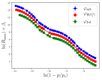
In addition to studying the final mass of the resulting black hole, we follow Garfinkle and Duncan (1998) and calculate the maximum Ricci scalar at the center of the collapse for subcritical evolutions. In Fig. 2 we plot as a function of along with a fit using Eq. (V.1) for the initial data studied. We again offset the plots vertically by amounts to aid readability. In this case we find critical exponents , , and , which are comparable to the values for mass scaling and to the accepted value in spherically symmetric critical collapse, .
V.2 Echoing
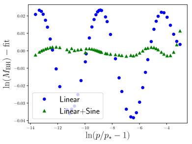
Having studied the scaling we now turn to the fine structure and echoing of the critical behavior. Echoing of any gauge-invariant quantity was described by Eq. (3) above. A small-amplitude sinusoidal modulation about the straight line expected from critical behavior was conjectured and observed in Hod and Piran (1997). Fig. 1 and 2 both show this feature. In Fig. 3 we plot the residuals when fitting only the linear term and when fitting the linear plus sine term for the spherically symmetric mass scaling case.111The residuals of the fits for non-spherical initial data and for Ricci scaling are qualitatively identical. The sinusoidal modulation is much clearer in Fig. 3 than in Fig. 1.
From the fit, Eq. (V.1), we estimate the period, . In Hod and Piran (1997) it was found that the relationship between the echoing period, and the scaling period, is . To test this relationship, we calculate using and also by estimating it directly from the Ricci scalar at the origin as a function of the logarithmic time, . is the proper time at the origin given by
| (38) |
and is the accumulation time of the self-similar solution.
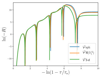
We find that despite being able to resolve the fine structure and knowing to six significant figures, the estimate of from the apparent horizon formation time is only accurate to about two digits. This is because the formation time of an apparent horizon is a gauge-dependent quantity. We estimate by assuming that the logarithmic time between successive echoes becomes constant and adjusting until this is true. The resulting is consistent with what we estimate from apparent horizon formation times. In Fig. 4 we plot , a geometric invariant, which shows the expected echoing that has been studied in previous work Garfinkle and Duncan (1998); Sorkin and Oren (2005). From Fig. 4 we estimate the echoing period to be .
| Initial Data | |||
|---|---|---|---|
In Table 1 we summarize and compare direct estimates of to . Specifically, we find that , near the best known value of Gundlach (1997a). For simulations that do not form a horizon, where we compute from the Ricci scalar scaling plot, Fig. 2, we find that , , and . The discrepancy between from mass scaling and Ricci scalar scaling is currently not understood. When studying the echoing of , we find , where the larger error is explained by the difficulty in estimating .
A power spectrum analysis shows that the spherical mode dominates the evolution. We define the power in a given -mode as
| (39) |
where is the number of radial points, and are the coefficients in spectral expansion. This definition is consistent with Parseval’s theorem given that
| (40) |
Also note that with this definition at a given radius
| (41) |
For the data we find that initially
| (42) |
or that approximately 18 percent of the power is in the mode. For the 3-d initial data we find that initially
| (43) |
or that approximately 35 percent of the power is in the mode.
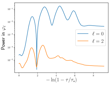
In Fig. 5 we plot the power in for for the initial data. Fig. 5 shows that the mode decays much more rapidly than the mode, suggesting that the spherically symmetric critical solution is approached. However, given the different initial data and that we are further from the critical solution than Choptuik et al. (2003), we are unable to corroborate or dispute their results.
The initial data used in Baumgarte (2018) is given by
| (44) |
The deformation in this case is proportional to the spherical harmonics as opposed to the spherical harmonic. Ref. Baumgarte (2018) found that for the critical behavior differs significantly from that of the spherically symmetric evolutions. For example, the critical exponent is observed to be . The percentage of the power in the mode for is approximately 47 percent. This is 12 percent more than our 3-d initial data that has behavior consistent with the spherically symmetric evolutions. This raises the question as to whether the reason Baumgarte (2018) see different behavior is because of the increased power in the modes or because the initial data is proportional to the spherical harmonics instead of the spherical harmonic. Work is underway to attempt to resolve this question.
VI Conclusions
We present results of a study of critical behavior in the 3-d gravitational collapse of a massless scalar field with no symmetry assumptions. We are able to resolve the dominant critical behavior as well as the fine structure in both supercritical and subcritical evolutions. We use the Spectral Einstein Code, SpEC SpE to perform the evolutions, with several key changes to the gauge condition and constraint damping. We study how the critical exponent and echoing period obtained from the data depend on how close to the critical solution the simulations are, as well as how the simulations are distributed in parameter space. This is especially important in 3-d where simulations are costly to perform. We find the critical exponents to be , , and , consistent with the accepted result in spherical symmetry of Gundlach (1997a). The accepted value of the echoing period in spherical symmetry is Gundlach (1997a), while we find echoing periods for all initial data consider. The discrepancy can be attributed to the difficulty in directly measuring the echoing period. We also test the predicted relationship Gundlach (1997a); Hod and Piran (1997) between the echoing period and the fine structure of the scaling, . We find that for mass scaling , , and , where is the period of the sinusoidal fine structure.
The agreement of the critical exponent, echoing period, and fine structure between the spherically symmetric and highly non-spherical simulations leads us to conclude that even for initial data far from spherical symmetry the critical solution is that of spherical symmetry. However, the reason why our results differ from those of Choptuik et al. (2003) and Baumgarte (2018), where data far from spherical symmetry approaches a different critical solution, is not yet fully understood. One reason for the discrepancy could be that in our data approximately 18 percent of the total power is in the mode for the initial data and 35 percent for the initial data, while in Baumgarte (2018) approximately 47 percent of the power is in the mode. In other words, more power than we used is needed in the mode. Another possible reason is that Baumgarte (2018) studied initial data while we study initial data. Work is underway to understand if either of these scenarios are responsible for the discrepancy and to independently reproduce the simulations of Baumgarte (2018).
VII Acknowledgements
We are grateful to Andy Bohn, François Hébert, and Leo Stein for insightful discussions and feedback on earlier versions of this paper. We are also grateful to the anonymous referee for the feedback. This work was supported in part by a Natural Sciences and Engineering Research Council of Canada PGS-D grant to ND, NSF Grant PHY-1606654 at Cornell University, and by a grant from the Sherman Fairchild Foundation. Computations were performed on the Zwicky cluster at Caltech, supported by the Sherman Fairchild Foundation and by NSF award PHY-0960291.
*
Appendix A Choosing parameter values for simulations
When estimating the error in the critical exponent and , we find it important to not only consider the error obtained from convergence tests, but also to study how and depend on the number of data points, and how close to the data points are. The former should be thought of as whether or not the space is sampled densely enough by the simulations. While reducing this error requires more (potentially costly) simulations, these simulations will be similar in their dynamics to simulations that have already been performed and so no algorithmic changes to the code are generally required. Determining how the closeness to affects and is a closely related, but separate issue. We study both of these sources of errors separately, while error estimates from convergence tests are included as error bounds on in the fits.
We use two methods to estimate the errors from our sampling of the space. First, we use bootstrapping to study how choosing different data points from within the datasets alters the critical exponent and . Second, we build a minimal grid that achieves the desired error tolerances by using a greedy algorithm. If the minimal grid is the same as or quite close to our grid we deduce that our grid may not be sufficiently dense to accurately extract and . We will now outline these methods in more detail.
The goal of bootstrapping is to resample the dataset randomly to obtain knowledge about how well the dataset represents the full population. This is done by randomly selecting as many points as there are in the dataset, while allowing repetition. Eq. (V.1) is then fit to the randomly selected points to obtain the critical exponent and . By repeating this procedure many times (we choose 10,000 times) we are able to plot a histogram of the critical exponents and values of . The variance in both and is then obtained by fitting a Gaussian to the histograms.
Using bootstrapping we find that the critical exponents obtained from mass scaling are left unchanged to within error with values , , and . For Ricci scaling, we find that the critical exponents also do not change within error, but the error estimate from bootstrapping is larger by approximately an order of magnitude than from the fit to the full dataset. The values obtained for from Ricci scaling are , , and . For we find qualitatively similar results to the critical exponent. Using data points from mass scaling we find , , and and from Ricci scaling we find , , and .
A greedy algorithm is designed to find the approximate global minimum of a problem by selecting the path that is a local minimum at each node in the decision tree. In this case we seek the optimal values of to determine and . Assume we have a minimal dataset that allows the fitting procedure to succeed. Then the greedy algorithm randomly selects a new value of and computes the corresponding black hole mass using Eq.(V.1). If adding the computed black hole mass to the dataset decreases the error it is added, otherwise a new value of is selected and added if it decreases the error in and . This is repeated until the error in and is below some specified tolerance.
The greedy algorithm method takes as input a range of in which to sample points, as well as the fit parameters obtained from a numerical study, i.e. , and . Fake black hole masses are computed using (V.1) and adding a random offset of at most to simulate numerical errors that would be present in the numerical simulations. The algorithm initially randomly chooses five (or six if also fitting for ) data points on the specified interval of . Next, points are randomly added until the fitting algorithm successfully identifies fit parameters. Then data points are randomly chosen and added to the dataset only if they reduce . Data points are added until .
Using the greedy algorithm, we find that for roughly 11 evenly spaced data points are necessary to achieve the desired tolerance and for approximately 15 evenly spaced data points are necessary. This is far fewer than the roughly 40 to 50 data points used for the fits to the numerical simulations. One reason for the difference in the number of data points is that, as indicated by the greedy algorithm results, initially when we do not know very accurately a denser grid is necessary to obtain a fit of decent accuracy. Another reason is that after finding to some accuracy we preformed simulations to fill a grid with spacing of approximately 0.1 in , which, in hindsight was unnecessary. Finally, a factor that was not accounted for in the greedy algorithm is that the fitting algorithm may not succeed because a good initial guess for the fit parameters is not known. The greedy algorithm always used the input that we modeled the data from.
To estimate the errors in and arising from how far from criticality the simulations are, we fit to only the lower or upper 25, 50 and 75 percent of data points. This provides insight into how many digits of the critical amplitude need to be resolved for the fits to be reliable. We note that this test only determines whether or not and are locally constant in space. The test cannot make any pdefinitive statements about and far outside this range, though this remains true regardless of how close to machine precision is.
By fitting to only a subset of the dataset, we observe that when fewer than two to three significant figures of are known, the linear + sine fit either fails to converge or else exhibits high sensitivity to the initial guess of the fitting parameters. However, the linear fit is still robust in this regime. Ultimately, we find that knowing to five or more significant figures provides robust fit results and good accuracy of the local critical exponent and , while knowing to fewer digits can lead to convergent fits that are biased by not having sufficiently resolved the sinusoidal oscillation.
References
- Choptuik (1993) M. W. Choptuik, Phys. Rev. Lett. 70, 9 (1993).
- Gundlach (1997a) C. Gundlach, Phys. Rev. D55, 695 (1997a), arXiv:gr-qc/9604019 [gr-qc] .
- Garfinkle and Duncan (1998) D. Garfinkle and G. C. Duncan, Phys. Rev. D58, 064024 (1998), arXiv:gr-qc/9802061 [gr-qc] .
- Garfinkle et al. (1999) D. Garfinkle, C. Cutler, and G. C. Duncan, Phys. Rev. D60, 104007 (1999), arXiv:gr-qc/9908044 [gr-qc] .
- Bland et al. (2005) J. Bland, B. Preston, M. Becker, G. Kunstatter, and V. Husain, Class. Quant. Grav. 22, 5355 (2005), arXiv:gr-qc/0507088 [gr-qc] .
- Sorkin and Oren (2005) E. Sorkin and Y. Oren, Phys. Rev. D71, 124005 (2005), arXiv:hep-th/0502034 [hep-th] .
- Taves and Kunstatter (2011) T. Taves and G. Kunstatter, Phys. Rev. D84, 044034 (2011), arXiv:1105.0878 [gr-qc] .
- Deppe et al. (2012) N. Deppe, C. D. Leonard, T. Taves, G. Kunstatter, and R. B. Mann, Phys. Rev. D86, 104011 (2012), arXiv:1208.5250 [gr-qc] .
- Golod and Piran (2012) S. Golod and T. Piran, Phys. Rev. D85, 104015 (2012), arXiv:1201.6384 [gr-qc] .
- Choptuik et al. (1996) M. W. Choptuik, T. Chmaj, and P. Bizon, Phys. Rev. Lett. 77, 424 (1996), arXiv:gr-qc/9603051 [gr-qc] .
- Gundlach (1997b) C. Gundlach, Phys. Rev. D55, 6002 (1997b), arXiv:gr-qc/9610069 [gr-qc] .
- Brady et al. (1997) P. R. Brady, C. M. Chambers, and S. M. C. V. Goncalves, Phys. Rev. D56, R6057 (1997), arXiv:gr-qc/9709014 [gr-qc] .
- Garfinkle et al. (2003) D. Garfinkle, R. B. Mann, and C. Vuille, Phys. Rev. D68, 064015 (2003), arXiv:gr-qc/0305014 [gr-qc] .
- Baumgarte and Montero (2015) T. W. Baumgarte and P. J. Montero, Phys. Rev. D92, 124065 (2015), arXiv:1509.08730 [gr-qc] .
- Gundlach and Baumgarte (2016) C. Gundlach and T. W. Baumgarte, Phys. Rev. D94, 084012 (2016), arXiv:1608.00491 [gr-qc] .
- Baumgarte and Gundlach (2016) T. W. Baumgarte and C. Gundlach, Phys. Rev. Lett. 116, 221103 (2016), arXiv:1603.04373 [gr-qc] .
- Gundlach and Baumgarte (2018) C. Gundlach and T. W. Baumgarte, Phys. Rev. D97, 064006 (2018), arXiv:1712.05741 [gr-qc] .
- Abrahams and Evans (1993) A. M. Abrahams and C. R. Evans, Phys. Rev. Lett. 70, 2980 (1993).
- Abrahams and Evans (1994) A. M. Abrahams and C. R. Evans, Phys. Rev. D49, 3998 (1994).
- Sorkin (2010) E. Sorkin, Phys. Rev. D81, 084062 (2010), arXiv:0911.2011 [gr-qc] .
- Sorkin (2011) E. Sorkin, Class. Quant. Grav. 28, 025011 (2011), arXiv:1008.3319 [gr-qc] .
- Hilditch et al. (2013) D. Hilditch, T. W. Baumgarte, A. Weyhausen, T. Dietrich, B. Brügmann, P. J. Montero, and E. Müller, Phys. Rev. D88, 103009 (2013), arXiv:1309.5008 [gr-qc] .
- Hilditch et al. (2016) D. Hilditch, A. Weyhausen, and B. Brügmann, Phys. Rev. D93, 063006 (2016), arXiv:1504.04732 [gr-qc] .
- Hod and Piran (1997) S. Hod and T. Piran, Phys. Rev. D55, 440 (1997), arXiv:gr-qc/9606087 [gr-qc] .
- Akbarian and Choptuik (2015) A. Akbarian and M. W. Choptuik, Phys. Rev. D92, 084037 (2015), arXiv:1508.01614 [gr-qc] .
- Martin-Garcia and Gundlach (1999) J. M. Martin-Garcia and C. Gundlach, Phys. Rev. D59, 064031 (1999), arXiv:gr-qc/9809059 [gr-qc] .
- Choptuik et al. (2003) M. W. Choptuik, E. W. Hirschmann, S. L. Liebling, and F. Pretorius, Phys. Rev. D68, 044007 (2003), arXiv:gr-qc/0305003 [gr-qc] .
- Healy and Laguna (2014) J. Healy and P. Laguna, Gen. Rel. Grav. 46, 1722 (2014), arXiv:1310.1955 [gr-qc] .
- Clough and Lim (2016) K. Clough and E. A. Lim, (2016), arXiv:1602.02568 [gr-qc] .
- Baumgarte (2018) T. W. Baumgarte, Phys. Rev. D98, 084012 (2018), arXiv:1807.10342 [gr-qc] .
- Lindblom et al. (2006) L. Lindblom, M. A. Scheel, L. E. Kidder, R. Owen, and O. Rinne, Class. Quant. Grav. 23, S447 (2006), arXiv:gr-qc/0512093 [gr-qc] .
- Pfeiffer and York (2003) H. P. Pfeiffer and J. W. York, Jr., Phys. Rev. D67, 044022 (2003), arXiv:gr-qc/0207095 [gr-qc] .
- Pfeiffer et al. (2003) H. P. Pfeiffer, L. E. Kidder, M. A. Scheel, and S. A. Teukolsky, Computer Physics Communications 152, 253 (2003), gr-qc/0202096 .
- (34) http://www.black-holes.org/SpEC.html.
- Scheel et al. (2009) M. A. Scheel, M. Boyle, T. Chu, L. E. Kidder, K. D. Matthews, and H. P. Pfeiffer, Phys. Rev. D79, 024003 (2009), arXiv:0810.1767 [gr-qc] .
- Szilagyi et al. (2009) B. Szilagyi, L. Lindblom, and M. A. Scheel, Phys. Rev. D80, 124010 (2009), arXiv:0909.3557 [gr-qc] .
- Hemberger et al. (2013) D. A. Hemberger, M. A. Scheel, L. E. Kidder, B. Szilágyi, G. Lovelace, N. W. Taylor, and S. A. Teukolsky, Class. Quant. Grav. 30, 115001 (2013), arXiv:1211.6079 [gr-qc] .
- Scheel et al. (2006) M. A. Scheel, H. P. Pfeiffer, L. Lindblom, L. E. Kidder, O. Rinne, and S. A. Teukolsky, Phys. Rev. D74, 104006 (2006), arXiv:gr-qc/0607056 [gr-qc] .
- Szilágyi (2014) B. Szilágyi, Int. J. Mod. Phys. D23, 1430014 (2014), arXiv:1405.3693 [gr-qc] .
- Lindblom and Szilagyi (2009) L. Lindblom and B. Szilagyi, Phys. Rev. D80, 084019 (2009), arXiv:0904.4873 [gr-qc] .