SPACE-TIME FRACTIONAL DIFFUSION IN CELL MOVEMENT MODELS WITH DELAY

Abstract

The movement of organisms and cells can be governed by occasional long distance runs, according to an approximate Lévy walk. For T cells migrating through chronically-infected brain tissue, runs are further interrupted by long pauses and the aim here is to clarify the form of continuous model equations that describe such movements. Starting from a microscopic velocity-jump model based on experimental observations, we include power-law distributions of run and waiting times and investigate the relevant parabolic limit from a kinetic equation for resting and moving individuals. In biologically relevant regimes we derive nonlocal diffusion equations, including fractional Laplacians in space and fractional time derivatives. Its analysis and numerical experiments shed light on how the searching strategy, and the impact from chemokinesis responses to chemokines, shorten the average time taken to find rare targets in the absence of direct guidance information such as chemotaxis.

(xxxxxxxxxx)

AMS Subject Classification: 92C17 (primary), 35K40, 35Q92, 35R11 (secondary)

1 Introduction

Modelling biological movement has received significant attention, with a large body of work devoted to deriving macroscopic (PDE) equations for the mean behaviour of some underlying microscopic movement model. A common description assumes movement follows a velocity-jump random walk, an alternating sequence of runs (movement with a fixed velocity) and reorientations (choosing a new velocity). When the movement is subject to an external bias, such as a chemical attractant, a series of studies dating to Patlak ³⁴ has generated solid understanding on how microscopic detail translates into a diffusion-advection type equation. ^{3; 32} Many derivations follow a fairly standard set of assumptions on individual behaviour, such as negligible waiting times between jumps and that the distribution of runtimes follows a Poisson distribution, as observed for classic studies on cells such as E. coli. ⁵ Under these assumptions, the macroscopic diffusion is of classic Fickian form.

Yet these assumptions do not apply universally, such as when searching for sparsely distributed targets. Recent years have witnessed reports on the tendency towards long-range diffusion, where a particle’s motion follows the characteristics of a Lévy flight: occasional non-localised flights that interrupt local movements. Intuitively, the probability of remaining stuck in non-productive regions decreases and the mean time taken to find rare targets is reduced. Non-Brownian search strategies have been reported for microorganisms, including E. coli ²⁴ and Dictyostelium, ²⁶ immune cells, ²⁰ and large organisms (e.g. mussels, ⁸ marine predators ^{21; 37} and monkeys ³⁶). The natural strategies have been adopted for robots. ²⁵

Motivated by the movements of immune cells in chronically infected brain tissue, ²⁰ here we derive the macroscopic model for a microscopic velocity-jump random walk (Section 3) in which both the runtime distance and waiting time between re-orientations follow long-tail (approximate Lévy) distributions. The delay is the key new ingredient from a modelling perspective, observed in experiments. ^{20; 31} We derive the appropriate kinetic-transport equation, where the “collision” term describes the nonlocal motion. Solving an equation for the resting population introduces a nonlocal delay in time for the moving population and, via a perturbation argument and appropriate space/time scaling, obtain the following nonlocal equation for the population density ($u_{\textnormal{tot}}$):

$${}_{t}^{C}\mathds{D}^{\kappa}u_{\textnormal{tot}}=\nabla\cdot\left(C_{\alpha,\kappa}\nabla^{\alpha-1}u_{\textnormal{tot}}\right)\ .$$ (1)

In the above, ${}_{t}^{C}\mathds{D}^{\kappa}$ is the fractional time derivative in the sense of Caputo, $\kappa\in(0,1)$, while $\nabla^{\alpha-1}$ denotes a fractional gradient for $\alpha\in(1,2)$, see the Definition in A.1. In the physical regime $\frac{\alpha}{\kappa}\in[1,2]$: this ranges from ballistic motion for $\alpha=\kappa=1$, with a resulting fractional heat equation governed by a Lévy process, to standard diffusion for $\alpha=2$, $\kappa=1$. The population is governed by a diffusion term with coefficient $C_{\alpha,\kappa}$ (defined at the end of Section 5) that represents a random component to motility. As described in greater detail below, experimental data on immune cell movements lead to $\alpha=1.15$ and $\kappa=0.7$. ²⁰ While our approach is often applied in the context of chemotaxis, it is noted that (1) does not contain a chemotactic component; this is in agreement with Ref. harris where the immune cells do not appear to exhibit directional migration on the experimental time/length scales.

The simple structure of Eq. (1) allows analytic insights not directly visible from the microscopic model. In particular, in Section 5.1 we explicitly write down the fundamental solution in $\mathbb{R}^{d}$ and, as direct applications, we discuss hitting and mean first passage times. Numerical experiments are presented in Section 6, allowing efficient quantitative description and a basis for parametric studies into immune cell search strategies.

2 Background and data

Toxoplasma gondii (T. gondii) is a species-crossing parasitic pathogen ⁶ with high seroprevalence in humans. Acute infection is followed by chronic infection, with the parasite taking up lifetime residence in the host’s central nervous system (CNS). While regarded as generally symptomless, infected individuals with compromised immune systems are at greater risk of life-threatening recurrence and chronic infection has also been linked to altered neurological behaviour. ³³ Long term immunity and control of chronic T. gondii infection primarily relies on CD8⁺ T cells, ²² which continuously search for and eliminate infected cells through contact. A recent study of CD8⁺ dynamics in infected brain tissue has revealed a number of insights into their chemical control and movement patterns. ²⁰ At a chemical level, the CXCL10/CXCR3 chemokine signalling system controls both the initial recruitment and subsequent maintenance of a CD8⁺ population ²⁰: anti-CXCL10 treatments lower the resident population of T cells and increase parasite densities. Further, CXCL10 appears to act as a chemokinetic agent during the chronic phase, with anti-CXCL10 treatment reducing average cell velocities. ²⁰

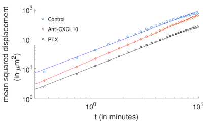
(a)

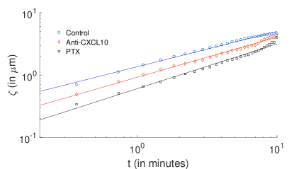
(b)

Figure 1: Reproduction of CD8⁺ T cell tracking data in ²⁰, indicating generalized Lévy diffusive behaviour in the central nervous system. (a) mean squared distance for $CD8^{+}$ T cells in control tissue (blue) and two treatments that impact on chemokine signalling (mice treated with anti-CXCL10 antibodies, red, and mice treated with PTX, a chemokine signalling inhibitor, black). (b) Spatial scaling factor of the self-similar diffusion.

Analyses of CD8⁺ T cell tracks in Ref. harris suggests that they follow a generalised Lévy walk. We reproduce the mean squared distances showing superdiffusive behaviour ($\langle x^{2}\rangle\sim t^{1.4}$) in Figure 1a. Yet, dependence of the spatial scaling on time (Figure 1b) is inconsistent with a Lévy walk in the absence of waiting times. In Ref. harris various models for T cell migration are examined, including random walks, persistent random walks and Lévy walks, with the conclusion that the experimental results are best described by a generalized Lévy walk. The microscopic description is as follows: (1) cells make straight runs with fixed velocity but random orientation, where the run distance is chosen randomly from a Lévy distribution ($L_{\mu}(\ell)\sim\ell^{-\mu}$) with exponent $\mu_{run}=2.15$; (2) following each run, cells pause for a time that is also distributed according to a Lévy distribution with exponent $\mu_{pause}=1.7$. Lévy distributions for the distance $\ell$ and times $\tau$ are drawn from the following expressions

$$Z_{\mu}=\frac{\sin((\mu-1)X)}{(\cos X)^{1/(\mu-1)}}\left(\frac{\cos((2-\mu)X)}{Y}\right)^{(2-\mu)/(\mu-1)}$$

where $X$ is a uniform random variable on the interval $[-\pi/2,\pi/2]$ and $Y=-\ln X^{\prime}$. For runs, once a distance $\ell$ is chosen, the walker moves in a randomly chosen direction for a time $\ell/v$, where $v$ is the velocity of the walker. For pauses, once a time $\tau$ is chosen, the walker remains stationary for that length of time.

While anti-CXCL10 treatments reduce CD8⁺ T cell speed and/or increase pauses, other migration statistics of the T cells remain the same: $\mu_{run}=2.15$ and $\mu_{pause}=1.7$, as in the control case. Thus, CXCL10 appears to operate as a chemokinetic agent through increasing the rate at which patrolling CD8⁺ T cells encounter their sparsely distributed targets, with CXCL10 (and other chemokines) shortening capture time through faster movement speeds. ²⁰

3 Microscopic model description

We model a population of CD8⁺ T cells moving in a medium in $\mathbb{R}^{n}$. It is noted that for the experimental system of Ref. harris, the resident T cell population numbers somewhere between $300,000$ and $450,000$ across a volume of $3.2-4.4\times 10^{11}\mu m^{3}$, motivating a continuum description for their collective movement. Microscopically, we assume each individual performs a generalized Lévy walk with the following properties:

1. The interactions between individuals are taken to be negligible. This assumption appears reasonable, given the relatively low densities of T cells.

2. Starting at position $\mathbf{x}$ and time $t$, we assume an individual runs in direction $\theta$ for some time $\tau$, called the “run time”. This run time is selected from a distribution $\psi$.

3. During runs, individuals are assumed to move with constant forward speed $c$ and take a straight line motion between reorientations.

4. Each time the individual stops it selects a new direction $\eta$ according to a distribution $k(\mathbf{x},t,\mathbf{\theta};\mathbf{\eta})$ which only depends on $|\theta-\eta|$, after waiting for some time $r$. The choice of new direction is taken to be independent of chemical concentrations/gradients.

5. The reorientation time $r$ follows a Lévy distribution $\psi_{r}(r)$.

Note that assumptions (3-4) derive from the experimental conditions of CD8⁺ T cells in Ref. harris: while the speed $c$ is a function of CXCL10, other walk statistics are unaffected. Without explicit data stating otherwise CXCL10 is assumed here to be (approximately) uniformly distributed at the spatial scale of observed tissue, and hence $c$ is taken as spatially constant. Investigations into the impact of anti-CXCL10 treatments can be recreated through changing the size of $c$.

3.1 Turn angle distribution

To describe the motion of T cells we assume, following Ref. harris, that the new direction is chosen independently of the target’s position. Thus, we take

$$k(\mathbf{x},t,\mathbf{\theta};\mathbf{\eta})=\ell(\mathbf{x},t,|\eta-\theta|)$$ (2)

where the new direction $\eta$ is symmetrically distributed with respect to the previous direction $\theta$, according to the symmetric distribution $\ell$. ² $|\eta-\theta|$ denotes the distance between two directions on the unit sphere $S$. More generally, immune cells can orient in response to environmental factors, such as attractant gradients or the structure of the extracellular matrix. In the absence of data suggesting that such guidance cues play any (significant) role in the behaviour observed in Ref. harris, we presently exclude this possibility.

3.2 Running probability and resting times

As described in Ref. harris, the motion of CD$8^{+}$ T cells is characterized by long runs, distributed according to a Lévy distribution, combined with resting times $r$. Within our microscopic description, we therefore assume the following power-law distribution for the running probability

$$\psi(\mathbf{x},\tau)=\left(\frac{\tau_{0}(\mathbf{x})}{\tau_{0}(\mathbf{x})+\tau}\right)^{\alpha}\ ,\ \textnormal{for}\ 1<\alpha<2\ ,$$ (3)

while resting times are distributed according to

$$\psi_{r}(r)=\left(\frac{r_{0}}{r_{0}+r}\right)^{\kappa}\ \textnormal{for}\ 0<\kappa<1\ .$$ (4)

$\psi$ describes the probability that a moving cell stops after time $\tau$. The resting time distribution, $\psi_{r}$, gives the probability that a cell does not move for a time $r$.

The running and waiting probabilities, $\psi$ and $\psi_{r}$, are related to the stopping and waiting frequency $\beta$ and $\beta_{r}$, via

$$\psi(\mathbf{x},\tau) =\exp\left(-\int_{0}^{\tau}\beta(\mathbf{x}+cs\theta,s)ds\right)\textnormal{and}$$ (5)

$$\psi_{r}(r) =\exp\left(-\int_{0}^{r}\beta_{r}(s)ds\right)\ .$$ (6)

Moreover, explicit expressions for both rates, $\beta(\mathbf{x},\tau)$ and $\beta_{r}(r)$, can be computed from the relations:

$$\beta(\mathbf{x},\tau) =\frac{\varphi(\mathbf{x},\tau)}{\psi(\mathbf{x},\tau)}=\frac{-\partial_{\tau}\psi}{\psi}=\frac{\alpha}{\tau_{0}+\tau}\ ,$$ (7)

$$\beta_{r}(r) =\frac{\phi(r)}{\psi_{r}(r)}=\frac{-\partial_{r}\psi_{r}}{\psi_{r}}=\frac{\kappa}{r_{0}+r}\ .$$ (8)

4 Modelling equations

Considering the assumptions in Section 3 and following the approach of Ref. alt1980biased, densities of moving $\sigma(\mathbf{x},t,\theta,\tau)$ and resting $\sigma_{0}(\mathbf{x},t,\theta,\tau)$ populations are described by the following system of equations:

$$(\partial_{\tau}+\partial_{t}+c\theta\cdot\nabla)\sigma(\cdot,\theta,\tau) =-\beta(\mathbf{x},\tau)\sigma(\cdot,\theta,\tau)\ ,$$ (9)

$$(\partial_{t}-\partial_{\tau})\sigma_{0}(\cdot,\theta,\tau) =T\beta(\mathbf{x},\tau)\sigma(\cdot,\theta,\tau)\ ,$$ (10)

$$\sigma(\cdot,\theta,0) =\sigma_{0}(\cdot,\theta,0)\ ,$$ (11)

where the dot denotes dependence in space, $\mathbf{x}$, and time $t$. Here the turn angle operator $T$, given by

$$T\phi(\eta)=\int_{S}k(\cdot,\mathbf{\theta};\mathbf{\eta})\phi(\theta)d\theta\ ,$$ (12)

describes the effect of changing from direction $\mathbf{\theta}$ to a new direction $\mathbf{\eta}$. The initial condition for the particles that start a new run at $\tau=0$ is given by

$$\sigma(\cdot,\eta,0)=\int_{0}^{t}\phi(r)\int_{0}^{t-r}d\tau\int_{S}\beta(\mathbf{x},\tau)\sigma(\mathbf{x},t-r,\theta,\tau)k(\cdot,\theta;\eta)d\theta dr\ .$$ (13)

The left hand side of equation (9) describes the temporal variation and transport of the density $\sigma(\cdot,\theta,\tau)$, while the right hand side gives the density of individuals that are left behind due to reorientation. These particles reappear in the resting mode described by (10), where stopping with frequency $\beta({\mathbf{x},\tau})$ eventually generates a new run ($\tau=0$) following a pause of some time $r$, with a probability given by the probability density function $\phi(r)$. This is described by equations (11) and (13).

Using the method of characteristics we find the solution of (9),

$$\sigma(\cdot,\theta,\tau)=\sigma(\mathbf{x}-c\theta\tau,t-\tau,\theta,0)\exp\left(-\int_{0}^{\tau}\beta(\mathbf{x}+cs\theta,s)ds\right).$$ (14)

We can rewrite expression (13) as

$$\sigma(\cdot,\eta,0)=\int_{S}k(\cdot,\theta;\eta)\left[\int_{0}^{t}d\tau\int_{0}^{t-\tau}\phi(r)\beta(\mathbf{x},\tau)\sigma(\mathbf{x},t-r,\theta,\tau)dr\right]d\theta\ ,$$ (15)

after changing the limits of integration. Then, integrating (9) and (10) with respect to $\tau$ and substituting (11) and (15), we obtain

$$\partial_{t}\bar{\sigma}+c\theta\cdot\nabla\bar{\sigma} =T\int_{0}^{t}\beta({\mathbf{x},\tau})\left(\int_{0}^{t-\tau}\phi(r)\sigma(\mathbf{x},t-r,\theta,\tau)dr\right)d\tau$$

$$-\int_{0}^{t}\beta(\mathbf{x},\tau)\sigma(\mathbf{x},t,\theta,\tau)d\tau\ ,$$ (16)

$$\partial_{t}\bar{\sigma}_{0} =T\int_{0}^{t}\beta(\mathbf{x},\tau)\sigma(\mathbf{x},t,\theta,\tau)d\tau$$

$$-T\int_{0}^{t}\beta({\mathbf{x},\tau})\left(\int_{0}^{t-\tau}\phi(r)\sigma(\mathbf{x},t-r,\theta,\tau)dr\right)d\tau\ .$$ (17)

Here $\bar{\sigma}$ and $\bar{\sigma}_{0}$ are defined as

$$\bar{\sigma}(\cdot,\theta)=\int_{0}^{t}\sigma(\cdot,\theta,\tau)d\tau,\ \ \bar{\sigma}_{0}(\cdot,\theta)=\int_{0}^{t}\sigma_{0}(\cdot,\theta,\tau)d\tau\ .$$ (18)

From (16) and (17) we can define the arrival rate of particles at a point $(\mathbf{x},t)$, after waiting for time $r$, as

$$j(\cdot,\theta)=\int_{0}^{t}\beta(\mathbf{x},\tau)\left(\int_{0}^{t-\tau}\phi(r)\sigma(\mathbf{x},t-r,\theta,\tau)dr\right)d\tau$$

and the density of cells leaving the point $\mathbf{x}$ for all times $\tau$ from $0$ to $t$, also called the escape rate, as

$$i(\cdot,\theta)=\int_{0}^{t}\beta(\mathbf{x},\tau)\sigma(\mathbf{x},t,\theta,\tau)d\tau\ .$$ (19)

Using (14) and the relations in (7), we can write

$$i(\cdot,\theta)=\int_{0}^{t}\mathcal{B}(\mathbf{x},t-s)\bar{\sigma}(\mathbf{x}-c\theta(t-s),s,\theta)ds\ ,$$

as derived in Ref. pks, where $\mathcal{B}$ is given, in the Laplace space

$$\hat{\mathcal{B}}(\mathbf{x},\lambda+c\theta\cdot\nabla)=\frac{\hat{\varphi}(\mathbf{x},\lambda+c\theta\cdot\nabla)}{\hat{\psi}(\mathbf{x},\lambda+c\theta\cdot\nabla)}+\textnormal{l.o.t.}.$$ (20)

To rewrite $j(\cdot,\theta)$ in terms of $\bar{\sigma}$ we use (14) again and let $s=t-\tau$. Hence,

$$j(\cdot,\theta) =\int_{0}^{t}\beta(\mathbf{x},\tau)\left(\int_{0}^{t-\tau}\phi(r)\sigma(\mathbf{x}-c\theta\tau,t-\tau-r,\theta,0)\psi(\mathbf{x},\tau)dr\right)d\tau$$

$$=\int_{0}^{t}\beta(\mathbf{x},t-s)\psi(\mathbf{x},t-s)e^{-(t-s)c\theta\cdot\nabla}\left(\int_{0}^{s}\phi(s-r)\sigma(\mathbf{x},r,\theta,0)dr\right)ds$$

$$=\int_{0}^{t}\varphi(\mathbf{x},t-s)e^{-(t-s)c\theta\cdot\nabla}\left(\phi(s)\ast\sigma(\mathbf{x},s,\theta,0)\right)ds\ .$$

Note that $j(\cdot,\theta)$ is still written in terms of $\sigma$ instead of $\bar{\sigma}$. So, taking the Laplace transform of $j(\cdot,\theta)$ and using the relation,

$$\hat{\bar{\sigma}}(\mathbf{x},\lambda,\theta)=\hat{\sigma}(\mathbf{x},\lambda,\theta,0)\hat{\psi}(\mathbf{x},\lambda+c\theta\cdot\nabla)$$

which was obtained from (18) and (14) (see Ref. pks for details), we can rewrite as,

$$\hat{j}(\mathbf{x},\lambda,\theta)=\hat{\varphi}(\mathbf{x},\lambda+c\theta\cdot\nabla)\hat{\phi}(\lambda)\hat{\sigma}(\mathbf{x},\lambda,\theta,0)=\frac{\hat{\varphi}(\mathbf{x},\lambda+c\theta\cdot\nabla)}{\hat{\psi}(\mathbf{x},\lambda+c\theta\cdot\nabla)}\hat{\phi}(\lambda)\hat{\bar{\sigma}}(\mathbf{x},\lambda,\theta)\ .$$

Equations (16) and (17) now can be written as

$$\partial_{t}\bar{\sigma}+c\theta\cdot\nabla\bar{\sigma} =T\int_{0}^{t}\mathcal{B}(\mathbf{x},t-s)\left(\int_{0}^{s}\phi(s-r)\bar{\sigma}(\mathbf{x}-c\theta(t-s),r,\theta)dr\right)ds$$

$$-\int_{0}^{t}\mathcal{B}(\mathbf{x},t-s)\bar{\sigma}(\mathbf{x}-c\theta(t-s),s,\theta)ds\ ,$$ (21)

$$\partial_{t}\bar{\sigma}_{0} =T\int_{0}^{t}\mathcal{B}(\mathbf{x},t-s)\bar{\sigma}(\mathbf{x}-c\theta(t-s),s,\theta)ds$$

$$-T\int_{0}^{t}\mathcal{B}(\mathbf{x},t-s)\left(\int_{0}^{s}\phi(s-r)\bar{\sigma}(\mathbf{x}-c\theta(t-s),r,\theta)dr\right)ds\ .$$ (22)

4.1 Scaling

Consider macroscopic space and time scales X and T respectively. We assume that the mean run time $\bar{\tau}$ and the mean waiting time $\bar{r}$ are small compared to the macroscopic time, i.e. $\bar{\tau}/\textsf{T}$ and $\bar{r}/\textsf{T}$ are equal to $\varepsilon^{\textnormal{power}}\ll 1$. We scale as follows,

$$t_{n}=\varepsilon t\ ,\ \mathbf{x}_{n}=\frac{\varepsilon\mathbf{x}}{s}\ ,\ c_{n}=\varepsilon^{-\gamma}c_{0}\ ,\ r_{n}=\varepsilon^{\varrho}r\ ,\ \textnormal{and}\ \tau_{n}=\tau\varepsilon^{\mu}\ ,$$ (23)

for $\mu>0$, $\gamma>0$ and $\varrho>0$. The scaling here is of parabolic type. It corresponds to a limit of the physical system with small average waiting and run times, small spatial run lengths, and large velocities compared to the macroscopic scales of an experiment. The values of the parameters $\gamma,\varrho,\mu$ are specified in Section 5.

Introducing this scaling we have,

$$\psi_{\varepsilon}(\mathbf{x},\tau)=\left(\frac{\varepsilon^{\mu}\tau_{0}}{\varepsilon^{\mu}\tau_{0}+\tau}\right)^{\alpha},\ \varphi_{\varepsilon}(\mathbf{x},\tau)=\frac{\alpha\left(\varepsilon^{\mu}\tau_{0}\right)^{\alpha}}{\left(\varepsilon^{\mu}\tau_{0}+\tau\right)^{\alpha+1}}$$

and

$$\phi_{\varepsilon}(r)=\frac{\kappa\left(\varepsilon^{\varrho}r_{0}\right)^{\kappa}}{(\varepsilon^{\varrho}r_{0}+r)^{\kappa+1}}\ .$$

Moreover, (21) is given by

$$\varepsilon\partial_{t}\bar{\sigma}+\varepsilon^{1-\gamma}c_{0}\theta\cdot\nabla\bar{\sigma} =T\int_{0}^{t}\mathcal{B}(\mathbf{x},t-s)\left(\int_{0}^{s}\phi_{\varepsilon}(s-r)\bar{\sigma}({\mathbf{x}-c\theta(t-s),r,\theta})dr\right)ds$$

$$-\int_{0}^{t}\mathcal{B}(\mathbf{x},t-s)\bar{\sigma}(\mathbf{x}-c\theta(t-s),s,\theta)ds\ .$$ (24)

Computing the Laplace transform of the above expression we obtain

$$\left(\varepsilon\lambda+\varepsilon^{1-\gamma}c_{0}\theta\cdot\nabla\right)\hat{\bar{\sigma}} (\mathbf{x},\lambda,\theta)-\varepsilon\bar{\sigma}^{0}(\mathbf{x},\theta)$$

$$\simeq-\left(\mathds{1}-\hat{\phi}_{\varepsilon}\left(\varepsilon\lambda\right)T\right)\hat{\mathcal{B}}_{\varepsilon}\left(\mathbf{x},\varepsilon^{1-\gamma}c_{0}\theta\cdot\nabla\right)\hat{\bar{\sigma}}(\mathbf{x},\lambda,\theta)\ ,$$ (25)

where we have assumed $\hat{\mathcal{B}}_{\varepsilon}(\mathbf{x},\varepsilon\lambda+\varepsilon^{1-\gamma}c_{0}\theta\cdot\nabla)\simeq\hat{\mathcal{B}}_{\varepsilon}(\mathbf{x},\varepsilon^{1-\gamma}c_{0}\theta\cdot\nabla)$ for $1>1-\gamma$.

The Laplace transform of the resting time density function $\phi_{\varepsilon}$, is given by

$$\hat{\phi}_{\varepsilon}(\varepsilon\lambda)=\kappa\left(a\lambda\right)^{\kappa}\Gamma(-\kappa,a\lambda)e^{a\lambda}$$

where $a=\varepsilon^{\varrho+1}r_{0}$. Using the following asymptotic expansion for the incomplete Gamma function ⁹

$$\Gamma(b,z) =\Gamma(b)\left(1-z^{b}e^{-z}\sum_{k=0}^{\infty}\frac{z^{k}}{\Gamma(b+k+1)}\right)\ ,$$ (26)

where $b$ is positive non-integer, and recalling that $b\Gamma(b)=\Gamma(b+1)$, we get

$$\hat{\phi}_{\varepsilon}(\varepsilon\lambda)=1-\varepsilon^{(1+\varrho)\kappa}r_{0}^{\kappa}\lambda^{\kappa}+\mathcal{O}(a\lambda)$$ (27)

since $0<\kappa<1$. Note that in the above we have considered $e^{a\lambda}=1+\mathcal{O}(a\lambda)$ and this approximation is valid for $(1+\varrho)\kappa>0$.

Hence, substituting (27) into (25) we obtain the following,

$$(\varepsilon\lambda+\varepsilon^{1-\gamma} c_{0}\theta\cdot\nabla)\hat{\bar{\sigma}}(\mathbf{x},\lambda,\theta)-\varepsilon\bar{\sigma}^{0}(\mathbf{x},\theta)$$

$$\simeq-\left(\mathds{1}-(1-r_{0}^{\kappa}\varepsilon^{(1+\varrho)\kappa}\lambda^{\kappa})T\right)\hat{\mathcal{B}}_{\varepsilon}\left(\mathbf{x},\varepsilon^{1-\gamma}c_{0}\theta\cdot\nabla\right)\hat{\bar{\sigma}}(\mathbf{x},\lambda,\theta)\ .$$ (28)

Transforming back to the $(\mathbf{x},t)$-space we get

$$\varepsilon\partial_{t}\bar{\sigma}(\cdot,\theta) +\varepsilon^{1-\gamma}c_{0}\theta\cdot\nabla\bar{\sigma}(\cdot,\theta)\simeq-(\mathds{1}-T)\mathcal{B}_{\varepsilon}(\mathbf{x},\varepsilon^{1-\gamma}c_{0}\theta\cdot\nabla)\bar{\sigma}(\cdot,\theta)$$

$$-r_{0}^{\kappa}\varepsilon^{(1+\varrho)\kappa}T{}_{t}\mathds{D}^{\kappa}\mathcal{B}_{\varepsilon}(\mathbf{x},\varepsilon^{1-\gamma}c_{0}\theta\cdot\nabla)\bar{\sigma}(\cdot,\theta)\ .$$ (29)

Here we have used the fact that the Laplace transform of the Riemann-Liouville fractional derivative ${}_{t}\mathds{D}^{\kappa}$ is given by Ref. klages2008anomalous

$$\mathcal{L}\left\{{}_{t}\mathds{D}^{\kappa}f(t)\right\}=\lambda^{\kappa}\hat{f}(\lambda)-\sum_{m=0}^{n-1}\lambda^{m}\lim_{t\rightarrow 0}{}_{t}\mathds{D}^{\kappa-m-1}f(0^{+})\ \textnormal{for},\ n-1<\kappa<n\ ,$$

where we assumed $f(0^{+})=0$, since there is no scattering at time zero.

Scaling (22) and changing the order of integration, the particles at rest satisfy the following equation

$$\varepsilon\partial_{t}\bar{\sigma}_{0}(\cdot,\theta) =T\int_{0}^{t}\mathcal{B}(\mathbf{x},t-s)\bar{\sigma}(\mathbf{x}-c\theta(t-s),s,\theta)ds$$

$$-T\int_{0}^{t}\phi_{\varepsilon}(t-s)\left(\int_{0}^{s}\mathcal{B}(\mathbf{x},t-s^{\prime})\bar{\sigma}(\mathbf{x}-c\theta(t-s^{\prime}),s^{\prime},\theta)ds^{\prime}\right)ds\ .$$ (30)

The Laplace transform of this expression is

$$\varepsilon\lambda\hat{\bar{\sigma}}_{0}(\mathbf{x},\lambda,\theta)-\varepsilon\bar{\sigma}^{0}_{0}(\mathbf{x},\theta)=r_{0}^{\kappa}\varepsilon^{(1+\varrho)\kappa}\lambda^{\kappa}T\hat{\mathcal{B}}_{\varepsilon}(\mathbf{x},\varepsilon^{1-\gamma}c_{0}\theta\cdot\nabla)\hat{\bar{\sigma}}(\mathbf{x},\lambda,\theta)\ ,$$ (31)

and if we assume that $1>1-\gamma$ as before we get

$$\varepsilon\partial_{t}\bar{\sigma}_{0}(\cdot,\theta)=r_{0}^{\kappa}\varepsilon^{(1+\varrho)\kappa}T{}_{t}\mathds{D}^{\kappa}\mathcal{B}_{\varepsilon}(\mathbf{x},\varepsilon^{1-\gamma}c_{0}\theta\cdot\nabla) \bar{\sigma}(\cdot,\theta)\ .$$ (32)

4.2 Conservation of particles

From the system (9)-(11) we can obtain a particle conservation equation, considering $\sigma_{\textnormal{tot}}(\mathbf{x},t,\theta)=\bar{\sigma}(\mathbf{x},t,\theta)+\bar{\sigma}_{0}(\mathbf{x},t,\theta)$, where $\bar{\sigma}$ and $\bar{\sigma}_{0}$ are given by (21) and (22) respectively. The conservation equation reads

$$\varepsilon\partial_{t}\int_{S}\sigma_{\textnormal{tot}}d\theta+\varepsilon^{1-\gamma}c_{0}\int_{S}\theta\cdot\nabla\sigma_{\textnormal{tot}}d\theta=0\ ,$$

where $S$ is the unit sphere. Hence, substituting (29) and (32) into the above expression we get

$$\varepsilon\partial_{t}\int_{S}\sigma_{\textnormal{tot}}d\theta +\varepsilon^{1-\gamma}c_{0}\int_{S}\theta\cdot\nabla\sigma_{\textnormal{tot}}d\theta=-\int_{S}(\mathds{1}-T)\mathcal{B}_{\varepsilon}(\mathbf{x},\varepsilon^{1-\gamma}c_{0}\theta\cdot\nabla)\bar{\sigma}d\theta$$

$$-r_{0}^{\kappa}\varepsilon^{(1+\varrho)\kappa}\int_{S}T\mathcal{B}_{\varepsilon}(\mathbf{x},\varepsilon^{1-\gamma}c_{0}\theta\cdot\nabla){}_{t}\mathds{D}^{\kappa}\bar{\sigma}(\mathbf{x},t,\theta)d\theta$$

$$+r_{0}^{\kappa}\varepsilon^{(1+\varrho)\kappa}\int_{S}T\mathcal{B}_{\varepsilon}(\mathbf{x},\varepsilon^{1-\gamma}c_{0}\theta\cdot\nabla){}_{t}\mathds{D}^{\kappa}\bar{\sigma}(\mathbf{x},t,\theta)d\theta=0\ .$$ (33)

Note that here we have used the conservation of particles during the tumbling phase given in (71). If we consider $\sigma_{\textnormal{tot}}(\mathbf{x},t,\theta)=\frac{1}{|S|}\left(\bar{u}+\bar{u}_{0}+\varepsilon^{\vartheta}n\theta\cdot\bar{w}\right)$ then we finally have

$$\varepsilon\partial_{t}(\bar{u}+\bar{u}_{0})+\varepsilon^{\vartheta+1-\gamma}nc_{0}\nabla\cdot\bar{w}=0\ ,$$ (34)

where

$$\bar{u}_{0}(\mathbf{x},t)=\frac{1}{|S|}\int_{S}\bar{\sigma}_{0}(\cdot,\theta)d\theta\ ,$$

and $\bar{u}$ and $\bar{w}$ are defined in Lemma A.1. The equation (34) is non-trivial only for $\vartheta=\gamma$.

We can define a new density, independent of the direction $\theta$, $u_{\textnormal{tot}}(\mathbf{x},t)=\bar{u}+\bar{u}_{0}$, that takes into account the moving and resting particles. Then, the conservation equation finally reads

$$\partial_{t}u_{\textnormal{tot}}+nc_{0}\nabla\cdot\bar{w}=0\ .$$ (35)

5 Fractional space-time equation

Next we obtain an expression for the mean direction $\bar{w}$, depending only on the density of moving particles $\bar{u}$.

Multiplying (29) by $\theta$ and integrating over all directions we obtain

$$n\varepsilon^{1+\gamma}\partial_{t}\bar{w} +\varepsilon^{1-\gamma}c_{0}\cdot\nabla\bar{u}\simeq-\frac{1}{|S|}\int_{S}\theta(\mathds{1}-T)\mathcal{B}_{\varepsilon}\left(\bar{u}+n\varepsilon^{\gamma}\theta\cdot\bar{w}\right)d\theta$$

$$-\frac{r_{0}^{\kappa}\varepsilon^{(1+\varrho)\kappa}}{|S|}\int_{S}\theta T\mathcal{B}_{\varepsilon}\ {}_{t}\mathds{D}^{\kappa}\left(\bar{u}+n\varepsilon^{\gamma}\theta\cdot\bar{w}\right)d\theta\ .$$ (36)

From equation (20) and for $\hat{\varphi}(\mathbf{x},\varepsilon^{1-\gamma}c_{0}\theta\cdot\nabla)$ and $\hat{\psi}(\mathbf{x},\varepsilon^{1-\gamma}c_{0}\theta\cdot\nabla)$ given as in Ref. pks we find

$$\mathcal{B}_{\varepsilon}=\frac{\varepsilon^{-\mu}(\alpha-1)}{\tau_{0}} -\frac{\varepsilon^{1-\gamma}c_{0}\theta\cdot\nabla}{2-\alpha}-\tau_{0}^{\alpha-2}\varepsilon^{\mu(\alpha-2)+(1-\gamma)(\alpha-1)}(1-\alpha)^{2}$$

$$\times\Gamma(-\alpha+1)(c_{0}\theta\cdot\nabla)^{\alpha-1}+\mathcal{O}\left(\tau_{0}^{\alpha-1}\varepsilon^{\mu(\alpha-1)}\lambda^{\alpha}\right)\ .$$ (37)

Substituting $\mathcal{B}_{\varepsilon}$ into (36), we compare the leading powers of $\varepsilon$. Considering that $(1+\varrho)\kappa>0$ as in Section 4.1, we observe that the terms involving the delay are of lower order with the exception of the term $\varepsilon^{-\mu+(1+\varrho)\kappa}{}_{t}\mathds{D}^{\kappa}\bar{u}$. The physically relevant scaling regime involves a fractional transport term in the expression for $\bar{w}$, hence we choose

$$\mu=\frac{1-\alpha(1-\gamma)}{\alpha-1}\ \textnormal{and}\ \gamma>1-\frac{1}{\alpha}\$$ (38)

to guarantee that $\mu>0$. Moreover, to ensure that the term involving a time delay is of lower order we also choose $(1+\varrho)\kappa>(\alpha-1)(\mu+1-\gamma)$. Taking these relations into account, the right hand side of (36) can be rewritten as

$$-\frac{1}{|S|} \int_{S}\theta(\mathds{1}-T)\Bigl{[}\varepsilon^{-\mu}\frac{(\alpha-1)\bar{u}}{\tau_{0}}-\varepsilon^{-\mu+\gamma}\frac{(\alpha-1)}{\tau_{0}}n\theta\cdot\bar{w}-\tau_{0}^{\alpha-2}\varepsilon^{\mu(\alpha-2)+(1-\gamma)(\alpha-1)}$$

$$\times(1-\alpha)^{2}\Gamma(-\alpha+1)(c_{0}\theta\cdot\nabla)^{\alpha-1}\bar{u}\Bigr{]}d\theta+\mathcal{O}\left(\varepsilon^{\min\{-\mu+(1+\varrho)\kappa,\ \mu(\alpha-1)\}}\right).$$ (39)

From the coefficient of the leading term $\varepsilon^{-\mu}$ in (39) we then obtain,

$$0=-\frac{1}{|S|}\int_{S}\theta(\mathds{1}-T)\frac{\alpha-1}{\tau_{0}}\bar{u}d\theta\ .$$ (40)

The subleading term is of order $\varepsilon^{\mu(\alpha-2)+(1-\gamma)(\alpha-1)}$ and we get

$$0 =-\frac{1}{|S|}\int_{S}\theta(\mathds{1}-T)\Bigl{(}\tau_{0}^{\alpha-2}(1-\alpha)^{2}\Gamma(-\alpha+1)c_{0}^{\alpha-1}(\theta\cdot\nabla)^{\alpha-1}\bar{u}$$

$$+\frac{n(\alpha-1)}{\tau_{0}}(\theta\cdot\bar{w})\Bigr{)}d\theta\ .$$ (41)

Note that we have obtained the same fractional diffusion equation as in Ref. pks and Ref. perthame2018fractional for a constant chemoattractant concentration.

From (41) we can obtain the mean direction $\bar{w}$ after applying the operator $T$ to the right hand side. Therefore, we obtain

$$\bar{w}=\frac{\pi\tau_{0}^{\alpha-1}(\alpha-1)}{\sin(\pi\alpha)\Gamma(\alpha)}\frac{(n^{2}\nu_{1}-|S|)}{n|S|(\nu_{1}-1)}c_{0}^{\alpha-1}\nabla^{\alpha-1}\bar{u}\ .$$ (42)

Substituting $\bar{w}$ into the conservation equation (35) we obtain

$$\partial_{t}u_{\textnormal{tot}}=\nabla\cdot\left(C_{\alpha}\nabla^{\alpha-1}\bar{u}\right)\ ,$$ (43)

where

$$C_{\alpha}=-\frac{n\pi\tau_{0}^{\alpha-1}(\alpha-1)}{\sin(\pi\alpha)\Gamma(\alpha)}\frac{(n^{2}\nu_{1}-|S|)}{n|S|(\nu_{1}-1)}c_{0}^{\alpha}>0\ \textnormal{for}\ 1<\alpha<2\ .$$

Next we write the right hand side of (43) in terms of $u_{\textnormal{tot}}$, and for this we return to the resting particles equation (32).

Expanding the right hand side of (32) and choosing only the leading terms we obtain, in the Laplace space,

$$\lambda\hat{\bar{\sigma}}_{0}(\mathbf{x},\lambda,\theta)-\bar{\sigma}_{0}^{0}(\mathbf{x},0,\theta)=r_{0}^{\kappa}\lambda^{\kappa}\frac{(\alpha-1)}{\tau_{0}}\hat{\bar{u}}+\mathcal{O}\left(\varepsilon^{(1+\varrho)\kappa+\mu(\alpha-2)+(\alpha-1)(1-\gamma)}\right)\ .$$

Here we have chosen $(1+\varrho)\kappa=\alpha(\mu+1-\gamma)$ which agrees with our previous assumption $(1+\varrho)\kappa>(\alpha-1)(\mu+1-\gamma)$. Integrating the above expression with respect to $\theta$ we can write it in terms of the Laplace transform of $\bar{u}_{0}$. Substituting $\bar{u}=u_{\textnormal{tot}}-\bar{u}_{0}$ into the right hand side and grouping terms we obtain

$$\hat{\bar{u}}_{0}(\mathbf{x},\lambda)-\frac{1}{\lambda}\bar{u}_{0}^{0}(\mathbf{x},0)=\frac{\hat{u}_{\textnormal{tot}}}{1+\frac{\tau_{0}}{r_{0}^{\kappa}(\alpha-1)}\lambda^{1-\kappa}}\ .$$ (44)

Since $\lambda\rightarrow 0$ then, applying a Taylor expansion and assuming all particles are moving at $t=0$, i.e. $\bar{u}_{0}^{0}=0$, we have

$$\hat{\bar{u}}_{0}=\left(1-\frac{\tau_{0}\lambda^{1-\kappa}}{r_{0}^{\kappa}(\alpha-1)}+\mathcal{O}\left(\lambda^{2(1-\kappa)}\right)\right)\hat{u}_{\textnormal{tot}}\ .$$ (45)

Substituting the inverse Laplace transform of (45) back into (43) we get

$$\partial_{t}u_{\textnormal{tot}} =\nabla\cdot\left(C_{\alpha}\nabla^{\alpha-1}(u_{\textnormal{tot}}-\bar{u}_{0})\right)$$

$$={}_{t}\mathds{D}^{1-\kappa}\nabla\cdot\left(C_{\alpha,\kappa}\nabla^{\alpha-1}u_{\textnormal{tot}}\right)$$ (46)

where

$$C_{\alpha,\kappa}=\frac{\tau_{0}}{r_{0}^{\kappa}(\alpha-1)}C_{\alpha}\ .$$

In fact, we can also write equation (46) using the Laplace transform as

$$\lambda^{\kappa}\hat{u}_{\textnormal{tot}}-\lambda^{\kappa-1}u_{\textnormal{tot}}^{0} =\nabla\cdot\left(C_{\alpha,\kappa}\nabla^{\alpha-1}\hat{u}_{\textnormal{tot}}\right)\ ,$$ (47)

and using the fact that

$$\mathcal{L}\left\{{}_{t}^{C}\mathds{D}^{\kappa}f(t)\right\}=\lambda^{\kappa}\hat{f}(\lambda)-\sum_{m=0}^{n-1}\lambda^{\kappa-m-1}f^{(m)}(0)\ ,$$

we have

$${}_{t}^{C}\mathds{D}^{\kappa}u_{\textnormal{tot}}=\nabla\cdot\left(C_{\alpha,\kappa}\nabla^{\alpha-1}u_{\textnormal{tot}}\right)\ .$$ (48)

Remark 5.1.

As previously noted, equation (48) does not contain a chemotactic component: this lies in agreement with Ref. harris, where CD8⁺ T cells do not exhibit directional migration on the time and length scales relevant to their experiments.

Remark 5.2.

From the analysis in the previous section, relevant scaling parameters satisfy the following relations:

$$\mu =\frac{1-\alpha(1-\gamma)}{\alpha-1}\ ,\ \varrho=\frac{\alpha\gamma}{\kappa(\alpha-1)}-1\ ,$$ (49)

for $0<\kappa<1$ and $1<\alpha<2$. From (38) and knowing that $\varrho>0$ we conclude that

$$\kappa-\frac{\kappa}{\alpha}<\gamma<1-\frac{1}{\alpha}\ .$$

For $\alpha=1.15$ and $\kappa=0.7$ as in ²⁰, $0.092<\gamma<1.15$. Choosing $\gamma=0.5$ then

$$\mu\approx 3.8\ \textnormal{and}\ \varrho\approx 4.47.$$

In this regime, the scaling of the long runs ($\mu$) and the scaling of the waiting times ($\varrho$) are of similar order.

5.1 Fundamental solution

Assuming that the stopping rate $\psi$ is independent of the position of the particle, we can write (48) as

$${}_{t}^{C}\mathds{D}^{\kappa}\ u_{\textnormal{tot}}=C_{\alpha,\kappa}\nabla\cdot\left(\nabla^{\alpha-1}u_{\textnormal{tot}}\right)=\widetilde{C}_{\alpha,\kappa}(-\Delta)^{\alpha/2}u_{\textnormal{tot}}.$$ (50)

Here, according to (76) in two dimensions, for $1<\alpha<2$,

$$\widetilde{C}_{\alpha,\kappa}=-2\sqrt{\pi}C_{\alpha,\kappa}\cos\left(\frac{\pi\alpha}{2}\right)\frac{\Gamma\left(\frac{\alpha+1}{2}\right)}{\Gamma\left(\frac{\alpha+2}{2}\right)}.$$

Following Ref. fundsol, the fundamental solution of (50) in $\mathbb{R}^{n}$, with initial condition $\delta_{0}$ and diffusion constant $C_{\alpha,\kappa}$,, can be found with the help of the Fourier-Laplace transform

$$\hat{\overline{G}}(\lambda,\xi)=\frac{\lambda^{\kappa-1}}{\lambda^{\kappa}+\widetilde{C}_{\alpha,\kappa}|\xi|^{\alpha}}.$$ (51)

Note that the Laplace transform of the Mittag-Leffler function is

$$\mathcal{L}\;E_{\kappa}(ct^{\kappa})=\frac{\lambda^{\kappa-1}}{\lambda^{\kappa}-c}.$$ (52)

Thus,

$$\hat{G}(t,\xi)=E_{\kappa}(-\widetilde{C}_{\alpha,\kappa}|\xi|^{\alpha}t^{\kappa}).$$ (53)

Using the formula for the inverse transformation of a radial function, we obtain

$$G(t,\mathbf{x})=\frac{|\mathbf{x}|^{1-n/2}}{(2\pi)^{n/2}}\int_{0}^{\infty}E_{\kappa}(-\widetilde{C}_{\alpha,\kappa}\tau^{\alpha}t^{\kappa})\tau^{n/2}J_{n/2-1}(\tau|\mathbf{x}|)d\tau,$$ (54)

where $J_{r}(z)$ is a Bessel function. Passing through the Mellin and inverse Mellin transform we conclude

$$G(t,\mathbf{x})=\frac{1}{\pi^{n/2}|\mathbf{x}|^{n}}H^{2,1}_{2,3}\left(\frac{|\mathbf{x}|^{\alpha}}{2^{\alpha}\widetilde{C}_{\alpha,\kappa}t^{\kappa}}\Big{|}^{(1,1);(1,\kappa)}_{(n/2,\alpha/2);(1,1);(1,\alpha/2)}\right)\ ,$$ (55)

where $H^{2,1}_{2,3}(z)$ is a Fox $H$-function. Useful identities and asymptotics may be found in Ref. Braaksma and Ref. Hbook. In particular by Theorem 3 in Ref. Braaksma for $1<\alpha<2,\;0<\kappa<1,\;\mathrm{and}\;\alpha<2\kappa$,

$$G(t,\mathbf{x})\simeq\frac{1}{|\mathbf{x}|^{n}}\ \left(\frac{|\mathbf{x}|^{\alpha}}{2^{\alpha}\widetilde{C}_{\alpha,\kappa}t^{\kappa}}\right)^{q}$$ (56)

when $\frac{|\mathbf{x}|^{\alpha}}{\widetilde{C}_{\alpha,\kappa}t^{\kappa}}\ll 1$, where $q=1$. In the limit $\frac{|\mathbf{x}|^{\alpha}}{\widetilde{C}_{\alpha,\kappa}t^{\kappa}}\gg 1$, we have $q=-1$. Note that these estimates hold in the regime of the experiments in Ref. harris discussed above, as well as for examples of superdiffusion without waiting times, ¹² relevant for certain studies of E. coli and Dictyostelium discoideum.

Other regimes generate the exponentially small tails known for Brownian motion, including the presence of waiting times. For example, for Brownian motion with waiting times, corresponding to $\alpha=2$ and $\kappa<1$, we obtain the fundamental solution

$$G(t,\mathbf{x})=\frac{1}{2\pi^{n/2}|\mathbf{x}|^{n}}H^{2,0}_{1,2}\left(\frac{|\mathbf{x}|}{2\sqrt{\widetilde{C}_{1,\kappa}}t^{\kappa/2}}\Big{|}^{(1,\kappa/2)}_{(1,1/2);(n/2,1/2)}\right)\ .$$ (57)

It has exponentially small tails as $|\mathbf{x}|t^{-\kappa/2}\to\infty$:

$$G(t,\mathbf{x})\simeq\frac{1}{|\mathbf{x}|^{n}}\left(\frac{|\mathbf{x}|}{2\sqrt{\widetilde{C}_{2,\kappa}}t^{\kappa/2}}\right)^{-\frac{n}{2-\kappa}}\exp\left(2(\frac{\kappa}{2}-1)\kappa^{\frac{\kappa}{2-\kappa}}\left(\frac{|\mathbf{x}|}{2\sqrt{\widetilde{C}_{2,\kappa}}t^{\kappa/2}}\right)^{\frac{2}{2-\kappa}}\right).$$ (58)

In particular, the range in which the asymptotics (56) holds shrinks to $0$ when $\alpha$ and $\kappa$ approach the boundary of the admissible region $1<\alpha<2,\;0<\kappa<1,\;\mathrm{and}\;\alpha<2\kappa$.

5.2 Hitting times

The fundamental solution of the continuum model derived in the previous subsection allows us to extract analytical approximations for biologically relevant quantities. As an example, we derive an expression for the time at which a particle hits some distant target $T$ with radius $a$, in the experimentally relevant regime $1<\alpha<2,\;0<\kappa<1,\;\mathrm{and}\;\alpha<2\kappa$. We seek the first time at which the density of the solution in $T$ reaches a certain threshold $\delta$. That is, we seek $t_{0}$ such that

$$\delta=\int_{T}\int_{\mathbf{R}^{n}}G(\mathbf{x}-\mathbf{y},t_{0})u_{0}(\mathbf{y})d\mathbf{y}d\mathbf{x}.$$ (59)

Assuming that the initial positions of the particles are given by $\mathbf{x}_{i}$, so that $u_{0}(\mathbf{x})=\sum_{i}\delta_{\mathbf{x}_{i}}(\mathbf{x})$, we obtain

$$\delta =\sum_{i}\int_{T}G(\mathbf{x}-\mathbf{x}_{i},t_{0})dx$$

$$=\sum_{i}\int_{T}\frac{1}{\pi^{n/2}|\mathbf{x}-\mathbf{x}_{i}|^{n}}H^{2,1}_{2,3}\left(\frac{|\mathbf{x}-\mathbf{x}_{i}|^{\alpha}}{2^{\alpha}\widetilde{C}_{\alpha,\kappa}t_{0}^{\kappa}}\Big{|}^{(1,1);(1,\kappa)}_{(n/2,\alpha/2);(1,1);(1,\alpha/2)}\right)\ d\mathbf{x}$$ (60)

If all initial positions are at distance $\gg(\widetilde{C}_{\alpha,\kappa}\tau^{\kappa})^{1/\alpha}$ from the target $T$, we may use the asymptotic expansion of the $H$-function from the previous subsection to obtain

$$\begin{split}\delta&\simeq\frac{2^{\alpha}\widetilde{C}_{\alpha,\kappa}t_{0}^{\kappa}}{\pi^{n/2}}\sum_{i}\int_{T}|\mathbf{x}-\mathbf{x}_{i}|^{-\alpha-n}d\mathbf{x}\\ &\simeq\frac{2^{\alpha}\widetilde{C}_{\alpha,\kappa}t_{0}^{\kappa}}{\pi^{n/2}}\mathrm{vol}(T)\sum_{i}|\mathbf{x}_{0}-\mathbf{x}_{i}|^{-\alpha-n},\end{split}$$ (61)

where $\mathbf{x}_{0}$ is a centre of the target $T$. Thus,

$$t_{0}\simeq\left(\frac{\delta\pi^{n/2}}{2^{\alpha}\widetilde{C}_{\alpha,\kappa}\mathrm{vol}(T)\sum_{i}|\mathbf{x}_{0}-\mathbf{x}_{i}|^{-\alpha-n}}\right)^{1/\kappa}.$$ (62)

This formula holds in the regime where the asymptotic expansion (56) is valid.

6 Numerical methods

In addition to the detailed qualitative information provided by the fundamental solution, the space-time fractional continuum equation allows efficient quantitative modelling of immune cell behaviour. We briefly describe the numerical approximation of the nonlocal operators. Challenges include the numerical evaluation of the singular integrals and the lack of boundary regularity, which leads to reduced convergence rates in naive approaches. Our numerical approximation of Equation (48) uses a finite element discretisation in space as discussed, for example, in Ref. VIPreprint and a time stepping method based on convolution quadrature as in Ref. acosta2017finite.

Let $\Omega\subset\mathbb{R}^{n}$ be a bounded domain with polygonal boundary and let $f\in C^{0}([0,T)\times\Omega)$. For $\alpha\in(1,2)$ and $\kappa\in(0,1)$, we consider the problem

$${}_{t}^{C}\mathds{D}^{\kappa}u+\nabla\cdot(C_{\alpha,\kappa}\nabla^{\alpha-1}u) =f \mathrm{in}\;\Omega\times[0,T)$$

$$u =0 \mathrm{in}\;\Omega^{c}\times[0,T)$$ (63)

$$u(\cdot,0) =u_{0} \mathrm{in}\;\Omega.$$

Let $\mathcal{T}_{h}$ be a shape regular and quasi-uniform triangulation of the region $\Omega$, with triangles of diameter at most $h$. Let $H_{h}$ be the subspace of piecewise linear functions of $H_{0}^{\alpha/2}(\Omega)$ associated with $\mathcal{T}_{h}$. Then, the semidiscrete weak formulation of the problem is as follows: Find $u_{h}\in C^{0}([0,T);H_{h})\cap C^{\kappa}([0,T);L^{2}(\Omega))$ such that

$$({}_{t}^{C}\mathds{D}^{\kappa}u_{h},v)+a(u_{h},v) =(f,v),$$ (64)

$$u_{h}(0) =u_{0},$$ (65)

for all $v\in H_{h}$. Here $a(\cdot,\cdot)$ represents the bilinear form

$$a(u,v)=(C_{\alpha,\kappa}\nabla^{\alpha-1}u,\nabla v)$$

of the fractional Laplacian and, for simplicity, we assume that $u_{0}\in H_{h}$. The discrete fractional Laplace operator $\Lambda_{h}$ is defined as the unique operator satisfying

$$(\Lambda_{h}u_{h},v_{h})=a(u_{h},v_{h}),\;\mathrm{for\;all}\;u_{h},v_{h}\in H_{h},$$ (66)

and the mass matrix $M_{h}$ is given by

$$(M_{h}u_{h},v_{h})=(u_{h},v_{h}),\;\mathrm{for\;all}\;u_{h},v_{h}\in H_{h}.$$ (67)

We conclude a strong reformulation of the semidiscrete problem: Find $u_{h}\in C^{0}([0,T);H_{h})\cap C^{\kappa}([0,T);L^{2}(\Omega))$ such that

$$M_{h}{}_{t}^{C}\mathds{D}^{\kappa}u_{h}+\Lambda_{h}u_{h} =f_{h} \mathrm{in}\;\Omega\times[0,T)$$ (68)

$$u_{h} =0 \mathrm{in}\;\Omega^{c}\times[0,T)$$

$$u(\cdot,0) =u_{0} \mathrm{in}\;\Omega\ .$$

For the discretisation of this equation in time we follow the approach of Ref. acosta2017finite. Dividing the time interval $[0,T)$ uniformly with time step $\tau=T/N$ of size $h^{\alpha/\kappa}$, we seek a numerical approximation of the convolution integral $K\ast g(t)$ associated with the Caputo time fractional derivative, by means of a finite sum as

$$K\ast g(t)=\int_{0}^{t}K(s)g(t-s)\mathrm{d}s\approx\sum_{j=0}^{n}w_{j}g(t-j\tau).$$ (69)

The weights $w_{j}$ are computed from the Taylor expansion of $\mathcal{K}(\delta(y)/\tau)$. Here, $\mathcal{K}$ is the Laplace transform of the kernel $K$ and $\delta(y)$ is the quotient of the generating polynomials of a multistep method. The $w_{j}$ are calculated from the recursion relation

$$w_{0} =\tau^{-\alpha/2},$$

$$w_{j} =\left(1-\frac{\alpha+2}{2j}\right)w_{j-1}.$$

For full details see Ref. Lubich1988_1 and Ref. Lubich_2.
The fully discrete time stepping scheme for (6) is then given as follows: Find $\{u_{h}^{1},u_{h}^{2},\dots\}\subset H_{h}$ such that

$$(w_{0}M+A)u_{h}^{n}=M\left((\sum_{j=0}^{n}w_{j})u_{h}^{0}-\sum_{j=1}^{n}w_{j}u_{h}^{n-j}+f_{h}^{n}\right),$$ (70)

where $u_{h}^{0}$ is given. $M,A$ are the mass and stiffness matrices related to the piecewise linear basis functions $\varphi_{i}$ of $H_{h}$ defined by $M_{ij}=(\varphi_{i},\varphi_{j}),\;A_{ij}=a(\varphi_{i},\varphi_{j})$, and $f_{h}^{n}=\sum_{i}(f(\cdot,n\tau),\phi_{i})\phi_{i}$ is the Galerkin projection of $f$ onto $H_{h}$ at time $n\tau$.

To illustrate the effect of the fractional derivative in time in the biologically relevant regime, we consider problem (6) in (a polygonal approximation of) $\Omega=B(0,10)$ with $f\equiv 0$ and $u_{0}(\mathbf{x})=\mathrm{max}(\exp(-5|\mathbf{x}|^{2})-0.2,0)$, using $h\simeq 0.025$ and $\tau\simeq h^{\alpha/\kappa}$. This setup corresponds to a Petri dish with an initial density of cells in the center. The domain is large enough so that the dominant effects correspond to diffusion rather than boundary effects, as in the experiment ²⁰. The solution at time $t=1$ is shown for $\alpha=1.15$ and $\kappa=0.7$ in Figure 2a and for $\alpha=1.15$ and $\kappa=1$ in Figure 2b. The figures clearly exhibit the memory effects induced by the fractional derivative in time.

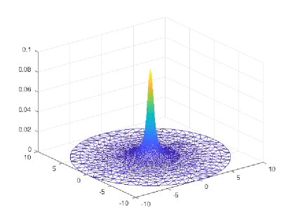
(a)

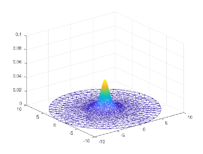
(b)

Figure 2: (a) Solution to (6) at time $t=1$ for $\alpha=1.15$, $\kappa=0.7$ (resting). (b) Solution to (6) at time $t=1$ for $\alpha=1.15$, $\kappa=1$ (no resting).

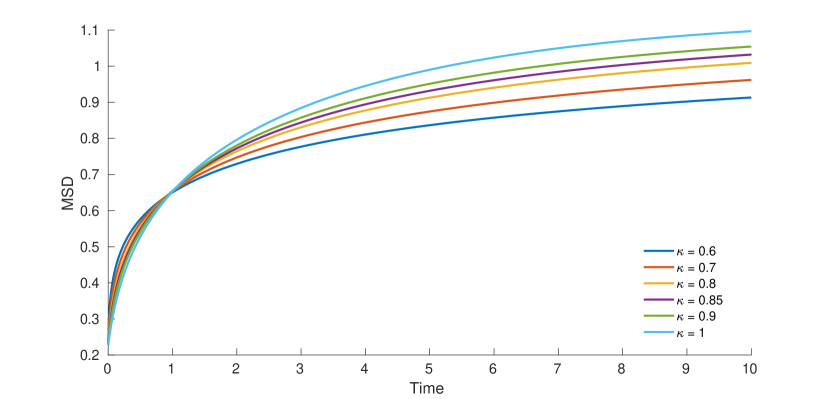
Figure 3: Width of solution depending on $\kappa$ as a function of time for $\alpha=1.15$.

Figure 3 shows the width of the cell density as a function of time for different $\kappa$.
Cross-sections of solutions of Equation (48) with initial condition given by $u(0,\mathbf{x})=\mathrm{max}(\exp(-5|\mathbf{x}|^{2})-0.2,0)$ are given in Figures 4 and 5, for time $t=0.02$. The time $t=0.02$ is chosen in order to exhibit the long tails of the Lévy diffusion, with their known slope. The influence of the boundary becomes more relevant for longer times. Figure 4 shows a cross section of the solution for values of $\kappa$ from $0.6$ to $1$, for the experimentally obtained $\alpha=1.15$ as in ²⁰. In particular, it depicts the expected tail of the density with decay $|\mathbf{x}|^{-n-\alpha}=|\mathbf{x}|^{-3.15}$, independent of $\kappa$, as well as the Markovian limit $\kappa\to 1$. Figure 5 varies the coefficient $\alpha$ from $1.15$ to $2$, for $\kappa=0.7$ as in Ref. harris. As long as $\alpha<2$, the density again decays like $|\mathbf{x}|^{-n-\alpha}$ away from the initial bump, while it exhibits the faster Gaussian decay for $\alpha=2$. As $\alpha\to 2^{-}$ the onset of algebraic decay is only visible on larger and larger spatial scales. We highlight the fact that the exponent of the decay does not depend on $\kappa$. This is due to the fact that the decay exponent of the fundamental solution for $|x|\to\infty$ depends only on $\alpha$, while it is independent of $\kappa$, see (56).

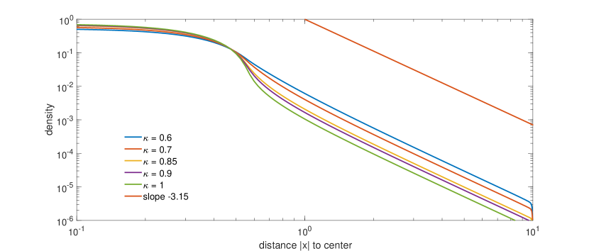
Figure 4: Cross-section of solution depending on $\kappa$ for $\alpha=1.15$.

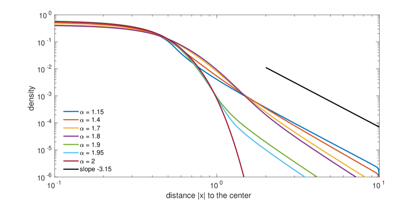
Figure 5: Cross-section of solution depending on $\alpha$ for $\kappa=0.7$.

7 Conclusions & Outlook

In this paper we have derived effective macroscopic diffusion equations for organisms exhibiting long-range behaviour and pauses. Beginning with a microscopic model in which run times and waiting times followed a power-law, as observed for certain T cell populations controlling chronic infections, we obtained a system of kinetic equations for the moving and resting particles. The fractional diffusion equation (48) emerges in a realistic limit.

The paper initiates a study into the interplay between long-range behaviour in space and long delays between runs, contributing to recent interest in anomalous diffusion processes. On the one hand, Lévy walks in space with short / negligible delays have been suggested for the movements of organisms such as E. coli under low nutrient levels and their macroscopic evolution has been shown to be described by fractional Patlak-Keller-Segel equations. ^{4; 12; 35} They have also inspired search strategies for swarm robotic systems.¹¹ On the other hand, Brownian motion with subdiffusive behaviour in time has been investigated in the context of death processes ¹⁴ or nonlinear interactions. ^{13; 38} A discussion of resting times in velocity-jump models is found in Ref. TaylorKing.

The macroscopic diffusion equation (48) permits analytical insights into the evolution of the density. For example, it reveals that the microscopic description enters via three parameters: the exponents $\alpha$ and $\kappa$ of the run and waiting times and the diffusion constant $C_{\alpha,\kappa}$. Chemotactic terms are of lower order: the long-range searching strategy is thus not disrupted by local gradient following. Of course, immune cells are well known for their responses to chemoattractants ¹⁹: in the context of the T cells studied here, it is possible that their detection of a local attractant gradient would trigger a conversion from long range searching behaviour to local gradient following.

The fundamental solution in $\mathbb{R}^{n}$, (55), provides an explicit formula for the probability distribution for the movement of a single particle. It leads to approximations for hitting times, (62), allows us to study the sensitivity to parameter changes and provides a step towards the analysis of mean first passage times, see below. On the other hand, Section 6 offers efficient and accurate numerical methods to employ the fractional PDE (48) for parametric studies, despite its nonlocal nature, and more extensive modelling is addressed elsewhere.

Figure 6: Hitting time $t_{0}$ as function of $\alpha$ and $\kappa$ in the range of validity of (62).

The experiments of Ref. harris specifically studied the effect of the CXCL10 concentration on T cell velocity: CD8⁺ T cells in mice treated with anti-CXCL10 were, on average, 23% slower than the cells of a control population with normal responses. From the fundamental solution of the space-time fractional equation we observe that velocity changes only alter the time scale of diffusion, corresponding to $c^{\frac{\alpha}{\kappa}}$. Thus, for the experimentally determined values $\alpha=1.15$ and $\kappa=0.7$, a 23% reduction in the velocity would yield an approximately 35% reduction in the diffusion timescale, and hence less efficient searching. In the absence of data stating otherwise, here we have assumed the CD8⁺ T cells migrate in an environment with homogeneous CXCL10 levels, and therefore constant velocities $c$. More generally, it would be of high interest to explore the impact of spatially-dependent velocities, resulting from nonuniform chemical profiles. The microscopic modelling of such problems, however, appears to be challenging even for velocity-jump models with standard Brownian motion. The model could also be extended to include extra complexity. For example, in bacteria, the stopping probability is linked to molecular components, which could enter as internal variables. We refer to work in this direction by Perthame et al. ³⁵ for the run-and-tumble of bacteria including a biochemical pathway, and a more detailed discussion of the impact of including internal variables is provided in. ⁴⁰

In the context of organisms searching for targets, a basic quantity of interest is the mean first passage time. It is defined as the time taken for a moving organism to reach a target or, more formally ¹⁵ as

$$\mathcal{T}(\mathbf{x})=\int_{0}^{\infty}\int_{\Omega}p(\mathbf{x}^{\prime},t\mid\mathbf{x},0)d\mathbf{x}^{\prime}\ dt\ .$$

Here, $p(\mathbf{x}^{\prime},t\mid\mathbf{x},0)$ is the probability that the particle is at $\mathbf{x}^{\prime}$ at time $t$ provided that it was at $\mathbf{x}$ at time $0$, i.e. the Green’s function of the fractional equation. For the diffusion equation (48) two regimes have been considered in one dimension: For subdiffusion, $0<\kappa<1$ and $\alpha=2$, it was shown in Ref. yuste2004comment that $\mathcal{T}(\mathbf{x})\rightarrow\infty$ for a target in a bounded domain, while for superdiffusion, $\kappa=1$ and $1<\alpha<2$, $\mathcal{T}(\mathbf{x})$ is finite under the same conditions. ¹⁸ It is the nonlocality of the equation here that generates the challenge, raising as it does the possibility of “leapfrogging” a target. The analysis in higher dimensions remains open. ⁴¹

Motivated by the differential movement of cells in gray and white brain matter,¹⁶ upcoming work on interface problems will consider velocities that take different values in distinct regions of the domain. While our current article addresses uncorrelated run and waiting times, correlations between these are also of interest. In the special case of perfect correlations between run and waiting times the macroscopic limit coincides with the one obtained from a velocity jump model for a correspondingly reduced velocity. Weaker forms of correlation are an interesting topic for future research.

From a search-area coverage perspective, a long-tailed distribution of waiting times makes little sense: Figure 6 shows that waiting only increases the hitting time, and hence decreases the searching efficiency. Of course, such apparent contradictions can only be explained through considering the underlying problem: following a migration, T cells must spend a certain time controlling their local environment for any antigen presenting (i.e. infected) cells, often detected through direct cell-cell contact, and hence ‘waiting’ is an intrinsic component of the search/detection process. While we have followed the data of Ref. harris and assumed independence between the selection of run and wait times, it is of course possible that a link exists: for example, a T cell performs a thorough check of some environment (checks a large number of cells) before embarking on a long run. The extent to which such considerations impact on the subsequent PDE remain to be explored.

Appendix A Turn angle and fractional operators

This section specifies some basic spectral properties of the turn angle operator $T$ defined in (12). Because $\ell$ in (2) is a probability distribution, it is normalized to $\int_{S}\ell(\mathbf{x},t,|\theta-e_{1}|)d\theta=1$, where $e_{1}=(1,0,\dots,0)$. We immediately observe

$$\int_{S}(\mathds{1}-T)\phi d\theta=0$$ (71)

for all $\phi\in L^{2}(S)$. Biologically, (71) corresponds to the conservation of the number of organisms in the tumbling phase. We also require some more detailed information about the spectrum of $T$.

Lemma A.1.

Assume that $\ell$ is continuous. Then $T$ is a symmetric compact operator. In particular, there exists an orthonormal basis of $L^{2}(S)$ consisting of eigenfunctions of $T$.
With $\mathbf{\theta}=(\theta_{0},\theta_{1},...,\theta_{n-1})\in S$, we have

$$\phi_{0}(\theta) =\frac{1}{|S|} \nu_{0}=1,$$ is an eigenfunction to the eigenvalue (72)

$$\phi_{1}^{j}(\theta) =\frac{n\theta_{j}}{|S|} \nu_{1}=\int_{S}\ell(\cdot,|\eta-1|)\eta_{1}d\eta<1.$$ are eigenfunctions to the eigenvalue

Any function $\bar{\sigma}\in L^{2}(\mathds{R}^{n}\times\mathds{R}^{+}\times S)$ admits a unique decomposition

$$\bar{\sigma}=\frac{1}{|S|}\left(\bar{u}+n\mathbf{\theta}\cdot\bar{w}\right)+\hat{z},$$ (73)

where $\hat{z}$ is orthogonal to all linear polynomials in $\theta$. Explicitly,

$$\bar{u}(\mathbf{x},t)=\int_{S}\bar{\sigma}(\mathbf{x},t,\mathbf{\theta})\phi_{0}(\theta)d\theta,\ \bar{w}^{j}(\mathbf{x},t)=\int_{S}\bar{\sigma}(\mathbf{x},t,\mathbf{\theta})\phi_{1}^{j}(\theta)d\theta,$$

and $\bar{w}=(\bar{w}^{1},\dots,\bar{w}^{n})$.

We recall some basic definitions concerning fractional differential operators, as well as their relation to the turning operator $T$.

Definition A.1.

For $s\in(0,2)$ and $f\in C^{2}(\mathds{R}^{n})$ define the fractional gradient of $f$ as

$$\nabla^{s}f(\mathbf{x})=\frac{1}{|S|}\int_{S}\mathbf{\theta}\mathbf{D}_{\mathbf{\theta}}^{s}f(\mathbf{x})d\mathbf{\theta}=\frac{1}{|S|}\int_{S}\mathbf{\theta}(\mathbf{\theta}\cdot\nabla)^{s}f(\mathbf{x})d\mathbf{\theta},$$ (74)

where $\mathbf{D}_{\mathbf{\theta}}^{s}=(\mathbf{\theta}\cdot\nabla)^{s}$ is the fractional directional derivative of order $s$. The fractional Laplacian of $f$ is given by

$$\mathds{D}^{s}f(\mathbf{x})=\frac{1}{|S|}\int_{S}\mathbf{D}^{s}_{\mathbf{\theta}}f(\mathbf{x})d\mathbf{\theta}.$$ (75)

It is easily shown that in two dimensions, for $1<\alpha<2$,

$$\mathds{D}^{s}=-2\sqrt{\pi}\cos\left(\frac{\pi\alpha}{2}\right)\frac{\Gamma\left(\frac{\alpha+1}{2}\right)}{\Gamma\left(\frac{\alpha+2}{2}\right)}(-\Delta)^{\nicefrac{{s}}{{2}}}\ .$$ (76)

See Ref. meerschaert2006fractional for further information.

References

• 1 Gabriel Acosta, Francisco M Bersetche, and Juan Pablo Borthagaray. Finite element approximations for fractional evolution problems. arXiv preprint arXiv:1705.09815, 2017.
• 2 Wolgang Alt. Biased random walk models for chemotaxis and related diffusion approximations. Journal of Mathematical Biology, 9(2):147–177, 1980.
• 3 Nicola Bellomo. Modeling complex living systems: a kinetic theory and stochastic game approach. Springer Science & Business Media, 2008.
• 4 Abdel Bellouquid, Juanjo Nieto, and Luis Urrutia. About the kinetic description of fractional diffusion equations modeling chemotaxis. Mathematical Models and Methods in Applied Sciences, 26(02):249–268, 2016.
• 5 Howard C Berg, Douglas A Brown, et al. Chemotaxis in Escherichia coli analysed by three-dimensional tracking. Nature, 239(5374):500–504, 1972.
• 6 Nicolas Blanchard, Ildiko Rita Dunay, and Dirk Schlüter. Persistence of Toxoplasma gondii in the central nervous system: a fine-tuned balance between the parasite, the brain and the immune system. Parasite Immunology, 37(3):150–158, 2015.
• 7 Boele Lieuwe Jan Braaksma. Asymptotic expansions and analytic continuations for a class of Barnes-integrals. PhD thesis, Groningen., 1936.
• 8 Monique de Jager, Franz J Weissing, Peter MJ Herman, Bart A Nolet, and Johan van de Koppel. Lévy walks evolve through interaction between movement and environmental complexity. Science, 332(6037):1551–1553, 2011.
• 9 NIST Digital Library of Mathematical Functions. http://dlmf.nist.gov/, Release 1.0.14 of 2016-12-21. F. W. J. Olver, A. B. Olde Daalhuis, D. W. Lozier, B. I. Schneider, R. F. Boisvert, C. W. Clark, B. R. Miller and B. V. Saunders, eds.
• 10 Jun-Sheng Duan. Time- and space-fractional partial differential equations. Journal of Mathematical Physics, 46(1):013504, 2005.
• 11 Gissell Estrada-Rodriguez and Heiko Gimperlein. Swarming of interacting robots with Lévy strategies: a macroscopic description. arXiv preprint arXiv:1807.10124, 2018.
• 12 Gissell Estrada-Rodriguez, Heiko Gimperlein, and Kevin J Painter. Fractional Patlak-Keller-Segel equations for chemotactic superdiffusion. SIAM Journal on Applied Mathematics, 78:1155–1173, 2018.
• 13 Sergei Fedotov. Nonlinear subdiffusive fractional equations and the aggregation phenomenon. Physical Review E, 88(3):032104, 2013.
• 14 Sergei Fedotov, Abby Tan, and Andrey Zubarev. Persistent random walk of cells involving anomalous effects and random death. Physical Review E, 91(4):042124, 2015.
• 15 Crispin W. Gardiner. Handbook of stochastic methods for physics, chemistry and the natural sciences. 2004.
• 16 Alt Giese, Lan Kluwe, Britta Laube, Hildegard Meissner, Michael E Berens, and Manfred Westphal. Migration of human glioma cells on myelin. Neurosurgery, 38(4):755–764, 1996.
• 17 Heiko Gimperlein and Jakub Stocek. Space-time adaptive finite elements for nonlocal parabolic variational inequalities. preprint.
• 18 M Gitterman. Mean first passage time for anomalous diffusion. Physical Review E, 62(5):6065, 2000.
• 19 Jason W Griffith, Caroline L Sokol, and Andrew D Luster. Chemokines and chemokine receptors: positioning cells for host defense and immunity. Annual Review of Immunology, 32:659–702, 2014.
• 20 Tajie Harris et al. Generalized Lévy walks and the role of chemokines in migration of effector CD8+ T cells. Nature, 486(7404):545–548, 2012.
• 21 Nicolas E Humphries et al. Environmental context explains Lévy and Brownian movement patterns of marine predators. Nature, 465(7301):1066, 2010.
• 22 SuJin Hwang and Imtiaz A Khan. CD8+ T cell immunity in an encephalitis model of Toxoplasma gondii infection. In Seminars in Immunopathology, volume 37, pages 271–279. Springer, 2015.
• 23 Rainer Klages, Günter Radons, and Igor M Sokolov. Anomalous transport: foundations and applications. John Wiley & Sons, 2008.
• 24 Ekaterina Korobkova, Thierry Emonet, Jose MG Vilar, Thomas S Shimizu, and Philippe Cluzel. From molecular noise to behavioural variability in a single bacterium. Nature, 428(6982):574–578, 2004.
• 25 M. Krivonosov, S. Denisov, and V. Zaburdaev. Lévy robotics. arxiv, 1612.03997, 2016.
• 26 Liang Li, Simon F Nørrelykke, and Edward C Cox. Persistent cell motion in the absence of external signals: a search strategy for eukaryotic cells. PLoS one, 3(5):e2093, 2008.
• 27 Christian Lubich. Convolution quadrature and discretized operational calculus. I. Numerische Mathematik, 52(2):129–145, 1988.
• 28 Christian Lubich. Convolution quadrature and discretized operational calculus. II. Numerische Mathematik, 52(4):413–425, 1988.
• 29 Arakaparampil M Mathai, Ram Kishore Saxena, and Hans J Haubold. The H-function: theory and applications. Springer Science & Business Media, 2009.
• 30 Mark M Meerschaert, Jeff Mortensen, and Stephen W Wheatcraft. Fractional vector calculus for fractional advection–dispersion. Physica A: Statistical Mechanics and its Applications, 367:181–190, 2006.
• 31 Mark J Miller, Sindy H Wei, Ian Parker, and Michael D Cahalan. Two-photon imaging of lymphocyte motility and antigen response in intact lymph node. Science, 296(5574):1869–1873, 2002.
• 32 Hans G Othmer and Chuan Xue. The mathematical analysis of biological aggregation and dispersal: progress, problems and perspectives. In Dispersal, individual movement and spatial ecology, pages 79–127. Springer, 2013.
• 33 Alexandru Parlog, Dirk Schlüter, and Ildiko Rita Dunay. Toxoplasma gondii-induced neuronal alterations. Parasite Immunology, 37(3):159–170, 2015.
• 34 Clifford S Patlak. Random walk with persistence and external bias. The Bulletin of Mathematical Biophysics, 15(3):311–338, 1953.
• 35 Benoît Perthame, Weiran Sun, and Min Tang. The fractional diffusion limit of a kinetic model with biochemical pathway. Zeitschrift für angewandte Mathematik und Physik, 69(3):67, 2018.
• 36 Gabriel Ramos-Fernández, José L Mateos, Octavio Miramontes, Germinal Cocho, Hernán Larralde, and Barbara Ayala-Orozco. Lévy walk patterns in the foraging movements of spider monkeys (Ateles geoffroyi). Behavioral Ecology and Sociobiology, 55(3):223–230, 2004.
• 37 David W Sims et al. Scaling laws of marine predator search behaviour. Nature, 451(7182):1098, 2008.
• 38 Peter Straka and Sergei Fedotov. Transport equations for subdiffusion with nonlinear particle interaction. Journal of Theoretical Biology, 366:71–83, 2015.
• 39 Jake P. Taylor-King, Benjamin Franz, Christian A. Yates, and Radek Erban. Mathematical modelling of turning delays in swarm robotics. IMA Journal of Applied Mathematics, 80:1454–1474, 2015.
• 40 Chuan Xue, Hans G Othmer, and Radek Erban. From individual to collective behavior of unicellular organisms: recent results and open problems. In AIP Conference Proceedings, volume 1167, pages 3–14. AIP, 2009.
• 41 SB Yuste and Katja Lindenberg. Comment on “mean first passage time for anomalous diffusion”. Physical Review E, 69(3):033101, 2004.