The Three-Dimensional Spatial Distribution of Interstellar Gas in the Milky Way: Implications for Cosmic Rays and High-Energy Gamma-Ray Emissions

Abstract

Direct measurements of cosmic ray (CR) species combined with observations of their associated $\gamma$-ray emissions can be used to constrain models of CR propagation, trace the structure of the Galaxy, and search for signatures of new physics. The spatial density distribution of the interstellar gas is a vital element for all these studies. So far models have employed the 2D cylindrically symmetric geometry, but their accuracy is well behind that of the available data. In this paper, 3D spatial density models for the neutral and molecular hydrogen are constructed based on empirical model fitting to gas line-survey data. The developed density models incorporate spiral arms and account for the warping of the disk, and the increasing gas scale height with radial distance from the Galactic center. They are employed together with the GALPROP CR propagation code to investigate how the new 3D gas models affect calculations of CR propagation and high-energy $\gamma$-ray intensity maps. The calculations made reveal non-trivial features that are directly related to the new gas models. The best-fit values for propagation model parameters employing 3D gas models are presented and they differ significantly from the values derived with the 2D gas density models that have been widely used. The combination of 3D CR and gas density models provide a more realistic basis for the interpretation of non-thermal emissions from the Galaxy.

1. Introduction

The distribution of the interstellar gas is a key ingredient to any self-consistent model describing propagation of cosmic rays (CRs) and generation of non-thermal interstellar emissions. Propagation of CR species in the Galaxy and their interactions with the interstellar gas and radiation field produce changes in their composition and spectra due to fragmentation, secondary particle production, and energy losses (see Strong et al., 2007, for a review). Measurements of the spectra and composition of CR species are used to constrain the most important parameters of CR propagation models (e.g., Jóhannesson et al., 2016). Observations of the interstellar emissions generated through the production and decay of neutral pions and inverse Compton scattering of CR electrons off the interstellar radiation field (ISRF) provide a direct probe of the spatial densities and spectra of CR protons, helium, and electrons in distant locations (e.g., Abdo et al., 2009, 2010; Ackermann et al., 2011, 2012; Planck Collaboration et al., 2015; Ajello et al., 2016), far beyond the reach of direct measurements. The interpretation of these data requires well developed propagation models and a detailed knowledge of the spatial distribution of the interstellar gas in the Milky Way.

The interstellar gas consists mostly of hydrogen and helium with a number density ratio of approximately 10 to 1 (Ferrière, 2001), while heavier elements represent a negligible fraction of the total gas mass. Depending on its temperature, three forms of the hydrogen gas are distinguished: atomic (H i), molecular (H₂), and ionized (H ii) hydrogen, while helium remains mostly neutral due to its much higher first ionization potential. The H i component is the most massive, containing about 60% of the mass while H₂ and H ii contain 25% and 15%, respectively (Ferrière, 2001). The spatial density distribution of the three forms is also widely different. The H ii component is the most widespread with a large scale height perpendicular to the Galactic plane of a few hundred pc near the solar system and a relatively low number density. The H₂ component on the other hand has a scale height of few tens of pc near the solar system, is very clumpy, and contained mostly in high density molecular clouds. The distribution of the neutral H i gas is somewhat intermediate between those of the ionized and molecular components with a scale height of about a hundred pc near the solar system and a large filling factor. Little is known about the distribution of the helium component because it is only observable in one of its ionizing states. It is assumed that its distribution closely follows that of hydrogen.

The correlation between the high-energy $\gamma$-ray intensity and the column density of interstellar gas was well-established using the first $\gamma$-ray sky surveys by SAS-2 and COS-B satellites (Lebrun & Paul, 1979; Lebrun et al., 1983), and later confirmed by the EGRET telescope (Hunter et al., 1997). The intrinsic connection between CRs and energetic $\gamma$-rays inspired the development of the first self-consistent model for CR propagation and diffuse $\gamma$-ray emission and led to the establishment of the open-source GALPROP project in the mid-1990s (Moskalenko & Strong, 1998; Strong & Moskalenko, 1998; Moskalenko & Strong, 2000a, b; Strong et al., 2000; Vladimirov et al., 2011). Solving a system of $\sim 90$ coupled transport equations and calculating the resulting high-energy emissions within a single framework enables the self-consistent treatment of all CR-related data. From the very beginning of the project GALPROP has been capable of full 3D spatial and time-dependent propagation calculations, but the data quality and computational requirements limited usage of these capabilities. Thus the CR propagation and production of secondary particles due to the interactions in the ISM relied on 2D cylindrical symmetric models for the respective spatial densities.

The data from the Fermi–LAT, with its major improvements in sensitivity and statistics compared to earlier experiments, heralded a new era for studies of the high-energy interstellar emissions from the Milky Way. Ackermann et al. (2012) considered a grid of 128 CR propagation models and compared them against $\sim 2$ years of Fermi–LAT data to test the effects of variations of important model parameters, such as the radial distribution of the CR sources, the size of the propagation volume (the halo), and the spin temperature of the H i gas. The models were all constructed using a 2D (cylindrical symmetry) approximation for the CR propagation. While the models provide reasonable agreement with the data, residuals of the order of few tens of percent are visible on scales ranging from a few to tens of degrees over the sky. Some of these residuals are likely related to large-scale structure in the CR and ISM distributions that is not described by the 2D models, such as higher gas densities near the spiral arms and/or the presence of freshly accelerated CRs in the vicinity of their sources. Consequently, analyses of the Fermi–LAT data have inspired progress towards more detailed 3D models for the high-energy interstellar emissions: Johannesson et al. (2013), Johannesson et al. (2015), and Porter et al. (2017) using GALPROP, Kissmann et al. (2017) and Niederwanger et al. (2017) with the PICARD code, and Nava et al. (2017) with a Monte Carlo code. Only for the GALPROP-based modeling has both the 3D structure of the ISM and CR spatial density distributions been taken into account; other works employ 2D ISM models.

Most of the knowledge of the gas distribution in the Milky Way has been acquired from line emission and absorption data. For the H i component the 21-cm hyperfine line is employed, which is observed both in emission and absorption for a wide range of conditions in the ISM (Dickey & Lockman, 1990; Kalberla & Kerp, 2009). Using simplifying but realistic assumptions, the radiative transport equation for the line emission can be solved to directly relate the observations of the emission line to the column density of the H i gas (Kulkarni & Heiles, 1988). However, this requires information about the excitation temperature (hereafter, the so-called “spin temperature” $T_{S}$) of the emitting gas.

The distribution of $T_{S}$ has been studied using observations of the 21-cm line in absorption and found to range from a few tens of K to a few thousands of K, and to be strongly correlated with the kinetic temperature of the gas (Heiles & Troland, 2003; Strasser & Taylor, 2004; Dickey et al., 2009). This agrees with the idea that the H i gas exists as two separate and stable phases in the ISM: the warm neutral medium (WNM, $T$$\sim$ few thousand K) and the cold neutral medium (CNM, $T$$\sim$ few tens of K). The WNM has a larger filling factor and is generally more widely spread than the CNM that is more clumpy and has a smaller scale height, at least in the inner Galaxy. Recent 21-cm absorption studies toward the outer Galaxy indicate that the warm and cold components are well mixed in that region, most likely because of the smaller amounts of molecular gas (Dickey et al., 2009).

The distribution of H₂ is less well known because typical conditions in the cold ISM do not produce detectable line emissions. Other tracers must therefore be used to estimate its column density. The most common is the rotational transition line from the ¹²C¹⁶O (hereafter CO) molecule, which is the second most abundant molecule in the ISM after H₂. The formation conditions of CO are similar to those of H₂, and the line emissions are mostly excited through collisions between CO and H₂ molecules. It has been observationally shown that the integrated line intensity of the CO lines is almost linearly related to the column density of H₂. The linear conversion factor, $X_{\text{CO}}$ has been found to depend somewhat on both column density and temperature of the ISM (Bolatto et al., 2013). Other molecular tracers, such as OH or ¹³CO in dense clouds, can also be used, but they are generally less abundant and their observations are more difficult.

The Doppler shift of the line emission caused by differential movement of the interstellar gas in the Galaxy can be modeled to extract distance information. The most common method assumes that the gas is in cylindrical rotation around the GC, which is a technique that has been applied since the beginning of systematic line-emission surveys (Burton, 1988; Kalberla & Kerp, 2009). Even though this approach incorporates the main features of the gas motions, Burton (1988) pointed out that non-cylindrical streaming motions can cause significant perturbations to modeled line emission profiles. These streaming motions have been shown to be up to 30 km s^-1 using numerical simulations (Chemin et al., 2015) and comparisons with other distance estimators (Tchernyshyov & Peek, 2017). Streaming motions dominate the line profiles in the directions toward the GC and anti-center where cylindrical rotation causes negligible motion along the line of sight (LOS). In addition, thermal and turbulent motions cause line broadening at the level of a few km s^-1, up to more than 10 km s^-1 (Strasser & Taylor, 2004).

The line broadening seriously affects the distance resolution available using the Doppler shift velocity, effectively smearing the gas along the LOS. The resulting elongated features visible in many derivations of the Galactic distribution of interstellar gas (e.g., Nakanishi & Sofue, 2003) are sometimes referred to as “fingers of God” because they all point towards the location of the Sun. Some efforts have been made to correct for these inadequacies: Levine et al. (2006) added elliptical rotation in the outer Galaxy to account for inconsistencies observed around the Galactic anti-center and Kalberla et al. (2007) included decreased rotation for gas that is further above/below the Galactic disk, while Pohl et al. (2008) used hydrodynamical simulations to estimate the gas velocity fields to obtain distance estimates in the direction of the GC and used Gaussian profile fitting to account for the line broadening. Even for the latter work noticeable artifacts are evident from the deconvolution procedure that smears out features in the actual spatial distribution.

Studies indicate that dust and gas in the ISM are well mixed (e.g., Bohlin et al., 1978), and under certain assumptions, the dust column density can also be used as a tracer of the gas column density (e.g., Schlegel et al., 1998). More sensitive surveys of the stars in the Galaxy over large areas of the sky can allow the 3D structure of the gas to be probed through the observation of their light absorption by the dust, a so-called dust reddening effect (e.g., Schlafly et al., 2014). This method can be more reliable than the kinematic distance estimators for the emission lines and also works for directions toward the GC and anti-center. However, its application is currently limited because it depends upon observations of a large number of stars, and the light of more distant stars is absorbed by the total column density along the LOS and, therefore, is very faint. Estimates of the gas distribution with this method require an assumption about a conversion factor between the dust and gas column densities that has been shown to be dependent on the physical properties of the ISM (e.g., Planck Collaboration et al., 2015).

The techniques described above for deriving the distribution of the interstellar gas in the Galaxy have been extensively applied (e.g., Levine et al., 2006; Pohl et al., 2008; Schlafly et al., 2014; Nakanishi & Sofue, 2016; Marasco et al., 2017; Schlafly et al., 2017). However, their results are not very well suited for usage as the gas distribution to run with CR propagation codes. The major issue is that the distributions are usually incomplete with gaps along sight lines toward the GC; this is particularly prevalent for models derived via deconvolution of the line-emission survey data. The stellar absorption method is limited by the distance from the Sun that can be probed (typically extending only out to $\sim 10$ kpc), and by the sky coverage. Even with the full-sky coverage of the Pohl et al. (2008) work, there are still issues with artifacts caused by broadening of the line emissions.

In this paper a forward folding model fitting technique is employed to estimate the 3D structure of the gas. Continuity is enforced over the directions with limited distance information by using a parameterized model of the gas distribution. This approach resolves the issue of artifacts caused by smearing and allows for complex gas rotation models that can also be parametrized and tuned to the data. It also allows the complexity of the spatial structure to be easily controlled, as well as the effects that each individual modification has on propagation of CRs to be studied separately. The goal of this paper is to determine the distributions of H i and H₂ in the Milky Way, the most important gas components for modeling CR propagation, production of secondaries, and high-energy interstellar emissions. The H ii gas, which has lower number density and larger scale height, is significantly less important when modeling CR propagation and is not considered in this paper. The effects of 3D structure for the ISRF in combination with CRs and non-thermal interstellar emissions have been explored by Porter et al. (2017).

2. 3D modeling of the interstellar gas

2.1. Analysis method

A forward folding technique is used to derive the 3D structure of the atomic and molecular hydrogen. Parameterized models for both the gas densities and the velocity fields are tuned with a maximum-likelihood fit to H i and CO line-emission data (described below). The evaluations of the likelihood function are made with the GALGAS code, which is described in detail in Appendix A. A brief overview of the code is given here.

The GALGAS code is designed to take arbitrary 3D models for the gas density and its velocity field and integrate them along the LOS from a user-specified location (the Solar system in this paper) to create line-emission profiles that can be compared to data. The coordinate system is right handed with the Sun positioned at the positive $X$-axis at a distance $R_{\odot}=8.5$ kpc from the Galactic center, while the $Z$-axis is pointing towards the north Galactic pole. The $Z=0$ plane coincides with Galactic latitude $b=0^{\circ}$ and the $Y$-axis is parallel to the Galactic longitude $l=-90^{\circ}$. In this coordinate system the conversion from $(l,b,s)$ to $(X,Y,Z)$ is given by

$$X =R_{\odot}-s\cos(b)\cos(l),$$

$$Y =-s\cos(b)\sin(l),\quad\text{and}$$

$$Z =s\sin(b).$$

where $s$ is the distance along the LOS $(l,b)$. For each LOS, the code uses the velocity field projected onto the line of sight to create a projection from $s$ to Doppler-shifted velocity $v$ which is calculated as the difference in velocity at the origin and a point along the LOS. Using this projection from $s$ to $v$ the code integrates the gas density along the line of sight to calculate the column density of gas associated with each velocity bin and converts it to line emission as described below. The code accounts for turbulent and thermal motions by smoothing the resulting emission profiles with a Gaussian kernel.

Conversion of gas column densities for each velocity bin $v$ to an observed line intensity is necessary for comparison with data. For H i, it is assumed that within each distance bin $s$ the gas is homogeneous with a spin temperature $\bar{T}_{S}$ that is specified with a parametrized distribution:

$$\bar{T}_{S}(v)=\frac{\int_{v}T_{S}(X,Y,Z)ds}{\int_{v}ds}$$ (1)

where the integration is performed over distance bin $s$ associated with velocity bin $v$. The column density is turned into observed brightness using a formula by Kulkarni & Heiles (1988):

$$T_{b}(v)=\left[\bar{T}_{S}(v)-T_{0}(v)\right]\left[1-e^{-\tau(v)}\right],$$ (2)

where the optical depth is given by $\tau(v)=N_{\text{H\,{\sc i}}}(v)/C\bar{T}_{S}(v)$, $N_{\text{H\,{\sc i}}}(v)=\int_{v}n_{\text{H\,{\sc i}}}(X,Y,Z)ds$ is the column density of hydrogen, and $C=1.83\times 10^{18}$ cm^-2 K^-1 (km s^-1)^-1 is a constant. If multiple distance bins align within the same velocity bin along a LOS, the optical depth from distance bins between the observer and the current bin is also included. In this work the only background considered is the cosmic microwave background and the background temperature $T_{0}=2.66$ K is constant over the sky. The Galactic synchrotron continuum emission is non-negligible at 1420 MHz. Its 3D distribution is not well known and is difficult to explicitly account for in Eq. (2), and is therefore not included. Typical estimates (Sofue, 2017) will lead to the emission from H i from the Galactic disk being underestimated by $\sim 10$ K for the model presented in this paper. Meanwhile, the optically thin assumption is used when modeling the H i gas, which is implemented using a large constant value for $T_{S}(X,Y,Z)$. This assumption has a much larger effect on the estimated emission than neglecting the synchrotron continuum emission. Hence, the analysis in this paper provides a robust lower limit for the density distribution of H i gas.

For the molecular gas, the standard assumption that the column density of H₂ is linearly related to the integrated line emission of CO is used, $N_{\text{H}_{2}}(v)=X_{\text{CO}}(v)W_{\text{CO}}(v)$. Here $W_{\text{CO}}(v)$ is the integrated CO line emission over the velocity bin $v$ and $X_{\text{CO}}(v)$ is the linear conversion factor. This assumption of linear relation is entirely phenomenological and does not have a strong physical motivation. The CO emission is generally optically thick and the linear relation between $N_{\text{H}_{2}}$ and $W_{\text{CO}}$ may be caused by the prevalent conditions in the ISM (Glover & Mac Low, 2011).

This assumption leads to a simple relation for the number density of H₂:

$$n_{\text{H}_{2}}(X,Y,Z)=X_{\text{CO}}(X,Y,Z)\epsilon_{\text{CO}}(X,Y,Z)$$ (3)

where the linear conversion factor $X_{\text{CO}}(X,Y,Z)$ can depend on the position in the Galaxy and $\epsilon_{\text{CO}}$ is the CO volume emissivity. This greatly simplifies the modeling of the CO line emission because the quantity of interest becomes $\epsilon_{\text{CO}}(X,Y,Z)$, which is independent of $X_{\text{CO}}(X,Y,Z)$ and linearly related to the CO line emission,

$$W_{\text{CO}}(v)=\int_{v}\epsilon_{\text{CO}}(X,Y,Z)ds$$ (4)

However, propagation codes require the number density of the hydrogen gas and specification of $X_{\text{CO}}(X,Y,Z)$ is necessary. Common assumptions include a constant $X_{\text{CO}}$ throughout the Galaxy or a radially increasing $X_{\text{CO}}(R)$ that seems to be more consistent with $\gamma$-ray data (Ackermann et al., 2012).

The model parameters are tuned by maximizing the likelihood of the model given the data. Even though the data is assumed to be normally distributed with a specified uncertainty, a student-t likelihood is used. The student-t distribution has more weight in the tails of the distribution compared to the normal distribution and the likelihood is less affected by strong outliers in the data. This property of the likelihood is desired because the models used in the analysis are by design not able to recover the fine structure of the gas distribution. Generally, there are more data points with low or little emission than bright ones, so using the student-t likelihood de-weights the emission peaks allowing a simplified model to catch the basic features of the data without being biased by strong emission peaks that it cannot reproduce. Also, the emission peaks not accounted for by the model will be evident in the residuals for the longitude and latitude profiles, making it easier to identify were additional model refinement is needed. Using the student-t likelihood requires, in addition to the data uncertainty, specifying the number of degrees of freedom which is set to $\nu=100$ for this analysis. The exact value does not change the overall conclusions of this work, but smaller values generally result in smaller estimated total gas mass with comparatively smaller negative residuals, while larger values give higher gas masses with larger negative residuals. Comparison with likelihoods using normally distributed errors show that $\nu\gtrsim 10^{4}$ is needed before the student-t likelihood gives similar results.

2.2. Data

This paper employs the H i LAB survey (Kalberla et al., 2005) and the composite CO survey of Dame et al. (2001) for the model tuning. The data is re-binned to a HEALPix grid (Górski et al., 2005) using HEALPix order 7 for H i while order 8 is used for the CO data. The selected resolution on the sky is such that the spatial resolution at the GC is about 80 pc and 40 pc, respectively for CO and H i. This is enough to resolve the gradient of the gas distributions near the GC. The velocity resolution of both surveys is degraded to 2 km s^-1 velocity bins to reduce the needed computational resources. The lower velocity resolution does not strongly affect the results because it is still smaller than the characteristic line spread for CO and H i, which is assumed to be 6 km s^-1 and 10 km s^-1, respectively. These values were determined by examining the tail of the line emission close to the tangent point velocities in the inner Galaxy and are in reasonable agreement with the analysis of Marasco et al. (2017). Non-cylindrical motions of the gas dominate the Doppler shifts of the line emission in directions towards the GC and anti-center so the velocity information is ignored for longitudes $|l|<10^{\circ}$ and $170^{\circ}<l<190^{\circ}$ and only the total velocity integrated emission is compared. In those regions the uncertainty for the bins along each LOS is summed up in quadrature assuming that the uncertainties are independent.

The statistical uncertainty on the data is assumed to be constant over the entire sky. Values of 0.05 K for CO and 0.1 K for H i are used, which are consistent with the noise estimate for the original surveys taking into account the re-binning. Because the models are too simple to properly account for the fine structure in the data the statistical uncertainty of the model parameters is not of high importance and therefore neither is the exact value of the uncertainty on the data. However, some of the model parameters described below are common in both the CO and H i models and constrained by both data sets and it is thus important to have the relative uncertainty of the two datasets correct to avoid biasing the likelihood either way. The statistics of the two data sets are such that the much brighter H i emission dominates the likelihood.

The H i data is filtered to exclude high-velocity emission, and also emission from the Local Group galaxies (Large and Small Magellanic Clouds, M31, and M33). No attempt is made to correct for bright radio background sources because the resolution of the LAB survey is not sufficient to do that accurately. Only data with $|b|\leq 40^{\circ}$ is selected for the analysis because higher latitude emission is predominantly due to local clouds that are not elements of the models considered in this paper. The increased number of pixels used for the likelihood evaluation from including high-latitude data considerably increases the required computation without providing additional constraints for the parameters of the global model. The CO survey is filtered with the moment masking method of Dame (2011), significantly reducing noise in the data. No other filtering is performed on the CO data.

2.3. Model Components

The model components used in this work are: a warped disk with a scale height that varies with Galactocentric radius, a central bulge/bar, and 4 logarithmic spiral arms. To reduce the number of parameters many of the geometrical parameters are the same for both the H i and CO models. This includes the parameters controlling the warp of the disk, the radial increase in scale height, the shape of the bulge/bar, and the shape of the spiral arms. The physical motivation for this assumption is that these parameters are controlled by external processes and should affect both components of the gas in a similar way. The radial and vertical profiles of the spiral arms follow that of the disk to further reduce the number of parameters. The velocity field is modeled as cylindrical rotation using the rotation curve of Sofue et al. (2009) scaled to match the IAU-recommended Sun-GC distance of $R_{\odot}=8.5$ kpc and the rotation velocity of $v_{\odot}=220$ km s^-1 at the location of the solar system. The distance from the GC projected onto the $X$-$Y$ plane is calculated as $R=\sqrt{X^{2}+Y^{2}}$. The optically thin assumption is used for the H i data, which is effectively modeled using a large constant value for $T_{S}$ in Eq. (2). This provides a robust lower limit for the column density of H i gas.

Two functional forms of the radial profile for the number density of the disk and spiral arms are explored, an exponential disk with a central hole

$$f_{d}(R)=n_{d}e^{-(R-r_{s})/r_{0}}\left[1-e^{\left(-R/r_{h}\right)^{h_{i}}}\right],$$ (5)

where $r_{s}=8.0$ kpc, $n_{d},r_{0},r_{h},h_{i}$ are free parameters, and a cubic spline in logarithm of the number density $n(R)$ between the values at constant radii, $R=0,2,4,6,8,10,15,20$, and $50$ kpc. The radii are selected based on previously determined radial profiles for the H i and CO gas while minimizing the number of parameters (Gordon & Burton, 1976; Bronfman et al., 1988). The cubic spline provides more freedom but at the expense of more than double the number of parameters. When combined with the bulge/bar component described below, the number density at the two innermost radial points of the cubic spline is fixed to a small value.

The warp of the Galactic disk is modeled similarly to Levine et al. (2006):

$$z_{0}=w_{0}(R)+w_{1}(R)\sin\left(\Theta-\theta_{1}\right)+w_{2}(R)\sin\left(2\Theta-\theta_{2}\right)$$ (6)

where $\Theta=\tan^{-1}(Y/X)$ is the azimuthal angle. The radial dependence of the amplitudes $w_{i}(R)$ is modeled with a cubic spline between the constant radii: 0, 5, 10, 15, 20, and 50 kpc. While the warp is dominantly in the outer Galaxy the points in the inner Galaxy are used to account for small variations in the disk mid-plane as found by Bronfman et al. (1988). The zero modes, $\theta_{i}$, are assumed to be independent of the radius. The vertical profile of the disk is modeled as a function of $Z^{\prime}/z_{h}$, where $Z^{\prime}=Z-z_{0}$ is the distance from the central plane of the disk, and $z_{h}$ is the scale height of the disk. Several functions describing the vertical profile are tested, including an exponential, a Gaussian, and hyperbolic secant to the power of $2,1$, and $0.5$. To account for the increasing scale height in the outer Galaxy, its radial dependence is modeled as

$$z_{h}(R)=z_{s}e^{(R-r_{z_{0}})/r_{z}},$$ (7)

where $r_{z_{0}}=8.5$ kpc is a constant, and $z_{s},r_{z}$ are free parameters. The final disk model is thus

$$f_{d}(X,Y,Z)=f_{d}(R)f_{s}(R,Z^{\prime}),$$ (8)

where $f_{s}(R,Z^{\prime})$ is one of the scale functions describing the vertical profile of the disk.

The central bulge/bar component is parameterized with the function

$$f_{b}(X,Y,Z) =n_{b}e^{-R_{r}^{e_{i}}}R_{r}^{p_{i}}\quad\text{with}$$ (9)

$$R_{r} =\left(R^{\prime}/r_{b}+Z/z_{b}\right)^{-1},$$

$$R^{\prime} =\sqrt{\left(X^{\prime}\right)^{2}+\left(Y^{\prime}/0.3\right)^{2}},$$

$$X^{\prime} =X\cos(\theta_{b})+Y\sin(\theta_{b})+x_{0},$$

$$Y^{\prime} =-X\sin(\theta_{b})+Y\cos(\theta_{b}).$$

where $n_{b}$, $e_{i}$, $p_{i}$, $r_{b}$, $z_{b}$, and $x_{0}$ are free parameters while $\theta_{b}=-30^{\circ}$ is a constant. The lack of velocity and, therefore, distance information means that it is not possible to constrain $\theta_{b}$ using the method employed in this paper. The exact value chosen for $\theta_{b}$ will affect the other parameters of the bulge, but not the data-model agreement. The value of $\theta_{b}$ that we use is within the range of $-10^{\circ}$ (Freudenreich, 1998) to $-45^{\circ}$ (López-Corredoira et al., 2007) given in the literature. The rotation of the bulge/bar corresponds to its closest distance being at positive longitudes.

Table 1 Model parameters describing the radial and vertical distributions of the number density for the H i and CO models

Parameter	Value
Disk parameters for CO model
$n_{d}$, K km s-1 kpc-1	0.894
$r_{s}$, kpc	8.0
$r_{0}$, kpc	1.27
$r_{h}$, kpc	6.34
$h_{i}$, kpc	6.38
$z_{s,\text{CO}}$, kpc	0.103
Disk parameters for H i model
$n(R=8\,\text{kpc})\equiv n_{8}$, cm-3	0.160
$n(0\,\text{kpc})/n_{8}$	$1.72\times 10^{-6}$
$n(2\,\text{kpc})/n_{8}$	$0.284$
$n(4\,\text{kpc})/n_{8}$	$0.807$
$n(6\,\text{kpc})/n_{8}$	$1.19$
$n(10\,\text{kpc})/n_{8}$	$0.798$
$n(15\,\text{kpc})/n_{8}$	$0.477$
$n(20\,\text{kpc})/n_{8}$	$0.0457$
$n(50\,\text{kpc})/n_{8}$	$1.12\times 10^{-3}$
$z_{s,\text{H\,{\sc i}}}$, kpc	0.0942
Bulge parameters for CO model
$n_{b}$, K km s-1 kpc-1	47.8
$\theta_{b}$, rad	5.67
$x_{0}$, kpc	0.751
$r_{b}$, kpc	0.514
$z_{b}$, pc	6.43
$e_{i}$	0.647
$p_{i}$	1.18
Flare parameters (common)
$r_{z}$, kpc	6.94
$r_{z_{0}}$, kpc	8.5

Table 2Model parameters describing the disk warp

Parameter	Mode 0	Mode 1	Mode 2
$\theta$, rad	$\cdots$	4.61	2.73
$w(0\,\text{kpc})$, kpc	–0.0756	0.146	0.287
$w(5\,\text{kpc})$, kpc	–0.00819	–0.0520	–0.0192
$w(10\,\text{kpc})$, kpc	–0.0288	0.101	–0.00716
$w(15\,\text{kpc})$, kpc	0.0576	0.737	–0.00587
$w(20\,\text{kpc})$, kpc	0.767	1.71	0.587
$w(50\,\text{kpc})$, kpc	20	20	14.9

Table 3Model parameters describing the shape and number density of the spiral arms

Arm	$\alpha_{j}$	$r_{\text{min},j}$	$\theta_{\text{min},j}$	$\epsilon_{\text{CO}}(8\,\text{kpc})$	$n_{\text{H\,{\sc i}}}(8\,\text{kpc})$
No.		kpc	rad	K km s-1 kpc-1	cm-3
1	3.30	2.00	1.05	0.642	0.184
2	4.35	3.31	2.62	0	0.193
3	5.32	3.89	4.19	3.37	0.332
4	4.75	3.19	5.76	7.53	0.521

The spiral arms are purely logarithmic:

$$\theta_{j}(R)=\alpha_{j}\log\left(R/r_{\text{min},j}\right)+\theta_{\text{min},j},$$ (10)

where $\alpha_{j}$, $r_{\text{min},j}$ and $\theta_{\text{min},j}$ are parameters of the model. Values of $\alpha_{j}$ and $r_{\text{min},j}$ are tuned in the minimization procedure, while the starting angles $\theta_{\text{min},j}=-\pi/6+j\pi/2$ are held constant throughout. The pitch angle of the spiral arm can be determined using $\theta_{p,j}=\tan^{-1}(\alpha_{j}^{-1})$. The starting point of arms 2 and 4 are at the ends of the central bulge/bar. The arms have a Gaussian profile perpendicular to the locus traced by Eq. (10) with a scale of 0.6 kpc giving them a FWHM of $\sim 1.4$ kpc. The radial density distribution of each arm is assumed to be identical to that of the disk in each density model, but with independent normalization for each arm. The vertical scale height of the arms is the same as that of the disk for the respective gas component.

To ensure stable fits, the maximum-likelihood procedure is performed in several iterations using the best-fit values from the previous step as a starting point for the next. The initial fit is performed using the disk component only without the warp and radial increase in the scale height. The model complexity is then increased by fitting for additional parameters and components in the following order: the radial distribution of the vertical scale height, the central bulge/bar, the warp of the disk, and the spiral arms. Because of the number of parameters and computing time required, the selection for the different radial and vertical profiles is performed without inclusion of the warp and spiral arms.

2.4. Results

According to the maximum-likelihood values, the logarithmic cubic-spline radial profile is a better match for the H i number density profile, while the exponential disk with a central hole is preferred for the CO distribution. The central bulge/bar component is rejected by the fit for the H i model and subsequently excluded from the H i model. The best-fit vertical profile is the square root of the hyperbolic secant for the H i model, while for CO it is the square of the hyperbolic secant that gives the best fit of all the tested profiles.

The parameters and their best-fit values for the final models of H i and CO gas are listed in Table 1 for the radial and vertical number density distributions of the disk, in Table 2 for the warp describing the central plane of the disk, and in Table 3 for the spiral arm parameters. Because the combined model does not reproduce the fine structure of the data, statistical uncertainties are unimportant and not reported. The statistical uncertainties are in most cases less than 0.1%. Each parameter value is reported with 3 significant digits, or at the level of the statistical uncertainty, whichever has a fewer number of significant digits. The final models will be distributed with larger number of significant digits as supplementary material to the paper in XML form readable by the GALPROP¹ code version 56.

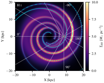
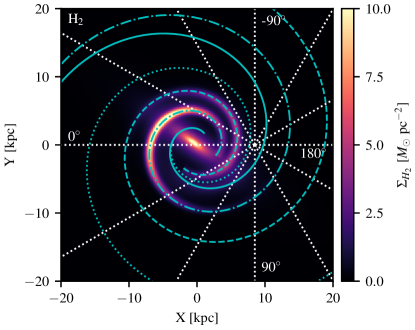
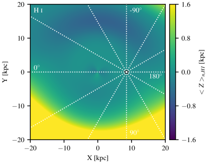
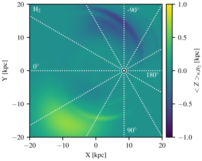
Figure 1.— Surface density maps for the final models (top) and maps of the first moment of the vertical density distribution (bottom). H i gas component is on left and H₂ component is on right. The CO number density is converted to H₂ number density assuming $X_{\rm CO}=2\times 10^{20}$ cm^-2 (K km s^-1)^-1. The Sun is marked as a white point and the white-dashed lines mark the longitude grid with 30^∘ step. The cyan curves on the surface density maps trace the cores of the spiral arms with each arm marked with a different line style: arm 1 is solid, arm 2 – dotted, arm 3 – dashed, and arm 4 – dash-dotted.

The best-fit model parameters are in reasonable agreement with previous studies of the interstellar gas. The radial distribution of the H i surface density is approximately flat between 4 and 15 kpc (Gordon & Burton, 1976). The distribution then falls off exponentially towards the outer Galaxy at a rate similar to that found by Kalberla & Dedes (2008). The CO distribution has a peak between 4 and 6 kpc (Bronfman et al., 1988) before falling off exponentially at larger Galactocentric distances. The central bulge/bar accounts for some part of strong CO emission in the inner Galaxy (Ferrière et al., 2007). The scale parameter for the disk flaring is somewhat smaller than that derived for the global average by Kalberla & Dedes (2008). The flaring parameter value is found to be closer to its value for the northern Galactic hemisphere indicating that northern latitudes ($b>0^{\circ}$) may have more weight when fitting the parameters of the described model. The warp parameters are in excellent agreement with those found by Levine et al. (2006) for Galactocentric radii between 10 and 25 kpc. The best-fit arm pitch angles are $16.8^{\circ}$ (arm 1), $12.9^{\circ}$ (arm 2), $10.6^{\circ}$ (arm 3), and $11.9^{\circ}$ (arm 4). These are all within the range of arm pitch angle estimates from the literature (e.g., Vallée, 2017).

The total masses of H i and H₂ gas components in the constructed models are $4.9\times 10^{9}$ M_⊙ (H i) and $0.67\times 10^{9}$ M_⊙ (H₂), where the standard value of $X_{\rm CO}=2\times 10^{20}$ cm^-2 (K km s^-1)^-1 (Bolatto et al., 2013) is used for the conversion. The spiral arms in the H i model account for approximately 25% of the mass while the remainder is in the disk. For the CO model the arms account for $\sim 42$% of the mass, the bulge/bar $\sim 31$%, and $\sim 27$% is in the disk component. These mass ratios may not relate directly to an estimated H₂ mass because the $X_{\text{CO}}$ conversion factor has been shown to depend on the specific properties of the ISM, and near the GC it may be an order of magnitude smaller than the Galactic average (Ferrière et al., 2007; Ackermann et al., 2012). For example, using $X_{\rm CO}=2\times 10^{19}$ cm^-2 (K km s^-1)^-1 for the bulge/bar component reduces the total H₂ mass in the model to $0.48\times 10^{9}$ M_⊙ and the fraction of the mass in the bulge/bar to $\sim 5$%.

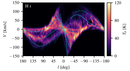
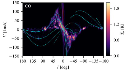
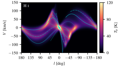
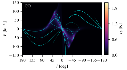
Figure 2.— Longitude-velocity diagram integrated over the longitude range $|b|<4^{\circ}$ for CO (left panels) and H i (right panels) gas. Top row shows the data, while bottom row shows our best-fit model. The cyan curves trace the cores of the spiral arms, the line coding is the same as in Figure 1.

The surface density maps of the final models

$$\Sigma(X,Y)=\int_{-\infty}^{\infty}n(X,Y,Z)dZ$$ (11)

are shown in Figure 1. The CO model has been converted to H₂ surface density using $X_{\text{CO}}=2\times 10^{20}$ cm^-2 (K km s^-1)^-1. The central bulge/bar and some spiral arms are clearly visible on the H₂ surface density map, meanwhile, the lack of arm 1 and the faint haze at the location of arm 2 are also apparent. Comparison of the spiral arm structures to the catalog of the spiral arm tangents collected by Vallée (2014) leads to the following identifications: arm 1 accounts for the Perseus arm, arm 2 – for Sagittarius and Carina, arm 3 – for Scutum and Crux-Centaurus, and arm 4 – for the 3 kpc arm, Norma, and Cygnus. Arm 3 also accounts for the new arm detected by Dame & Thaddeus (2011), which has been confirmed using parallax observations by Sanna et al. (2017). This picture is also mostly consistent with the updated spiral arm model presented by Vallée (2016). The starting points of the arms shown in his Figure 2 are at 2 kpc so care must be taken when matching the arms. The only exception is that arm 1 does not match the Perseus arm in the updated model of Vallée (2016).

The final arm parameter values are somewhat dependent on their initial values chosen for the model fit and their interpretation could be ambiguous. In particular, arm 1 does not match perfectly with the start of Perseus at $l=-23^{\circ}$; its start is closer to $l=-15^{\circ}$. It also overlaps with arm 2 in the inner Galaxy, indicating that there is some degeneracy between these arms. In turn, this may affect the derived values of the $\alpha_{j}$ parameters so the modeled spiral arms match observations in the outer Galaxy. The presented spiral arm configuration is quite stable over the relatively few choices of initial values tested in this analysis. The resulting small variations in the model parameters do not qualitatively affect the results for CR propagation and high-energy interstellar emission (Section 3) and further exploration of the model is deferred to future work.

To illustrate the warp of the Galactic disk, the first mode of the calculated vertical number density distribution

$$\left<Z\right>_{n}(X,Y)=\frac{\int_{-\infty}^{\infty}Zn(X,Y,Z)dZ}{\Sigma(X,Y)}$$ (12)

is shown in Figure 1. The results are in good agreement with those from Levine et al. (2006) (their Figure 11). In this work the same warp is applied to the disk and spiral arm components of the H i and CO models, but the central bulge/bar does not include any warp. The best-fit parameters for the CO model correspond to the bulge/bar component that falls off with the Galactocentric distance slower than the disk and spiral arm components. The bulge/bar contributes to the gas number density even outside the solar radius and the warp maps of the H i and CO models are not identical even though the warp component is the same for both models. The contribution of the bulge/bar component falls off more quickly along its minor axis in the plane resulting in larger values of the first mode along that direction. The warp is not significant for the CO model because its number density for distances $\gtrsim 10$ kpc is low. Even though the effect of the warp is small in the inner Galaxy it is found to be necessary for the model because it significantly improves the data-model agreement.

Figure 2 shows the longitude-velocity diagram for both models and data integrated over the Galactic disk $|b|<4^{\circ}$, with the locations of the spiral arms overlaid. Overall, the models reproduce the data fairly well, with the main “butterfly” shape of the model driven by the cylindrical rotation. The spiral arm structures are clearly visible in the H i model plot and their locations reasonably match similar structures in the data. However, the enforced smoothness of the models means that the true complexity of the observed ISM is not fully recoverable and even some large-scale features are not reproduced. There is a clear spur between the spiral arm structure visible to the right of $(l,V)=(100^{\circ},-60$ km s${}^{-1})$ in the H i data that is absent in the model. Gaps in the data near $(50^{\circ},-30$ km s${}^{-1})$ and $(-110^{\circ},30$ km s${}^{-1})$ show the absence of the gas, but correspond to the spiral arms in the model. Very bright emission near $(80^{\circ},0$ km s${}^{-1})$ and $(-90^{\circ},0$ km s${}^{-1})$ is not reproduced by H i nor CO models. The CO model is also much fainter than the data toward the inner Galaxy, and the few clouds visible in the outer Galaxy are not reproduced either.

Figure 2 also illustrates why the densities in spiral arms 1 and 2 are lower than in the other arms, especially for the CO model. Arm 1 (associated with the Perseus arm and shown as a solid curve) starts in a void in the data at around $l=15^{\circ}$. It then aligns with the location of arm 2 in a region with data and follows to some extent other evident features all the way to the outer Galaxy. It looks shifted relative to the brightest features in the data at $90^{\circ}<l<150^{\circ}$ in both CO and H i. Arm 1 ends up in a large void in the H i data at $l\sim-110^{\circ}$ before picking up some structure further on. There is also a bright feature near $(40^{\circ},40$ km s${}^{-1})$ in the CO data with corresponding structure in the H i data that may be associated with this spiral arm. The location of this feature is, however, offset from the modeled spiral arm. Arm 2 that has been associated with Sagittarius and Carina and shown as a dotted curve seems to be offset from a very bright feature in the H i data at $15^{\circ}<l<45^{\circ}$, and from a fainter feature at $-70^{\circ}<l<-20^{\circ}$. There is evidence of similar offsets in the CO data as well. The offsets mentioned above are likely caused by some combination of an incorrect spiral arm shape and/or variations in the velocity field. However, it is difficult to discriminate between these two effects without additional information.

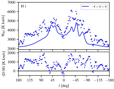
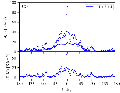
Figure 3.— Longitude profiles of the models (curves) overlaid on the data (points). The model and data are integrated over all velocity bins and averaged over the latitude range $|b|<4^{\circ}$. H i gas is on top and CO is at the bottom.

The longitude profiles (Figure 3) show that the data are under-predicted by the models. This is a consequence of using the student-t likelihood, which de-weights strong outliers in the data, in combination with a simplified and smooth model. The outliers are positive in almost all cases giving rise to positive residuals. Of the two, the H i model performs somewhat better at representing the data with the residuals fairly constant over the entire longitude range. The most conspicuous residuals are seen at $60^{\circ}\leq l\leq 160^{\circ}$ and $-100^{\circ}\leq l\leq-20^{\circ}$. The spiral arm tangents are fairly obvious in the models and coincide with corresponding peaks in the data profiles reasonably well indicating that the locations of the spiral arms in the model are mostly correct. Therefore, some of the discrepancies observed in the $l$-$V$ diagrams in Figure 2 are likely due to streaming motions of the gas that are unaccounted for in the models and can give rise to velocity discrepancies of more than 10 km s^-1. It is also likely that the assumption made in this paper of azimuthally independent radial distribution is not appropriate (Kalberla & Dedes, 2008). The residuals in the outer Galaxy for longitudes in the range $90^{\circ}\leq l\leq 180^{\circ}$ are larger than those for $-180^{\circ}\leq l\leq-90^{\circ}$ for both the H i and CO models. This indicates that the models are missing some structure in that region, possibly related to the Perseus arm.

The CO model is more strongly affected due to the clumpy nature of the CO emission visible in the $l$-$V$ diagram in Figure 2. About $\sim 50$% of the CO intensity for $|l|\leq 45^{\circ}$ is unaccounted for by the model, and there are positive residuals around $l\pm 90^{\circ}$. The very bright peak in CO emission toward the GC is also not reproduced by the bulge/bar structure. Outside these longitudes the CO model fares better mostly because the CO intensity is low toward the outer Galaxy. There is also the assumption of continuity for the spiral arms. It is not guaranteed that the spiral arms all follow a logarithmic shape throughout their distance. The arms are also assumed to all follow the same radial distribution in density which may not be the case. This has the effect that even though the fraction of the density contained in the spiral arms is higher in the best-fit CO model compared to the best-fit H i model, the peaks associated with the spiral arm tangents are less prominent in the CO model. There is clear lack of emission around the tangents of the Perseus arm at $l\approx-23^{\circ}$ and the Sagittarius-Carina arm at $l\approx 51^{\circ}$ and $l\approx-79^{\circ}$. The CO spatial distribution model developed is the initial attempt at decomposing the emission into spiral arms and disk components, given the methodology employed in this paper. Additional model tuning is required to improve the representation of the data, but this is deferred to future work.

3. Effects on CR propagation and high-energy $\gamma$-ray emission

3.1. The GALPROP code

The underlying concept of the GALPROP code is that all CR-related data, including direct measurements and indirect electromagnetic observations are related to the same Milky Way galaxy and should, therefore, be modeled self-consistently. With over 20 years of development it is the best known and most feature-rich code for calculations of CR propagation and their interactions in the Galactic ISM. The recently released GALPROP code version 56 (Porter et al., 2017) is used in this work. The latest releases are always available at the dedicated website¹, which also provides the WebRun facility to run GALPROP via a web browser interface. The website contains detailed information on CR propagation together with links to all GALPROP team publications and the supporting data sets required to run the code. The interstellar gas models developed in this paper will also become available at the above-mentioned website. A brief overview of the GALPROP code is given below, while further details can be found in recent GALPROP publications (e.g., Porter et al., 2017; Jóhannesson et al., 2016; Vladimirov et al., 2011, and references therein).

The GALPROP code numerically solves the diffusion-reacceleration equation for CR transport with a given source distribution and boundary conditions for all CR isotopes. Energy losses from ionization and Coulomb interactions are included for all species and for CR electrons and positrons energy losses due to Bremsstrahlung, inverse Compton (IC) scattering, and synchrotron emission are also included. Additional processes for nuclei include nuclear spallation, secondary particle production, radioactive decay, electron capture and stripping, electron knock-on, and electron K-capture. Electromagnetic radiation from the decays of $\pi^{0}$, $K^{0}$, and heavier mesons, Bremsstrahlung, IC scattering, and synchrotron emission are calculated self-consistently once the system of transport equations has been solved. To capture the finer structure of the interstellar gas the $\gamma$-ray intensity maps associated with interactions between CRs and the interstellar gas use the column density estimated from the line emission surveys that have been split into Galactocentric annular maps using the gas velocity field; see Appendix B of Ackermann et al. (2012) for full details of their construction. The GALPROP code has proven to be remarkably successful in modeling both CR data (e.g., Jóhannesson et al., 2016; Boschini et al., 2017) and electromagnetic radiation associated with CR interactions in the ISM (e.g., Ackermann et al., 2012; Ajello et al., 2016).

The spatial number density distribution of the interstellar gas is used in GALPROP for calculations of the production of secondaries and energy losses by CR species. In addition, the number density distribution is used internally for the proper weighting of the gas column density along the LOS in the individual Galactocentric gas rings for calculations of Bremsstahlung and $\pi^{0}$-decay $\gamma$-ray intensity maps. However, the density distribution is approximate and does not represent all details of the true distribution of the interstellar gas. Therefore, the ratios between the column densities estimated from the H i and CO line emission surveys and corresponding column densities from the Galactic gas distributions employed in GALPROP are used as multiplicative corrections for each LOS integration. This method enables GALPROP to predict the details in the structure of the gas-related interstellar emissions imprinted in the $\gamma$-ray skymaps without the necessity to develop precise 3D models of the gas distribution in the Galaxy. Even though all versions of GALPROP since the very beginning allowed full 3D functionality, including 3D gas distributions, the analytic 2D cylindrically symmetric gas distributions as described by Ackermann et al. (2012) have been most commonly used. This usage mode is attributed to the increased demand for computing resources required to run GALPROP in 3D mode as well as the absence of detailed 3D models of the ISM. The latest GALPROP (version 56) expands upon this functionality with the capability to read in the same XML description of the gas distribution used in the GALGAS code, and the optimizations made significantly improve the performance. The output from the analysis described in Section 2 can, therefore, be used directly without any modification.

3.2. CR propagation

This Section illustrates how the new 3D interstellar gas distributions affect the CR propagation parameters derived from a fit to the direct observations of primary and secondary CR species. This study is limited to models with diffusive reacceleration and an isotropic and homogeneous diffusion coefficient with a power-law rigidity dependence. The propagation parameters are tuned using the method described by Porter et al. (2017). To enable comparison with that work the same CR source density models, SA0, SA50, and SA100 are used. The CR source density distribution is composed of two constituents, a disk and 4 spiral arms, where each component has the same exponential scale height of 200 pc perpendicular to the Galactic plane. The source distribution in the disk follows the radial distribution of pulsars as given by Yusifov & Küçük (2004). The source distribution in the spiral arms matches the density distribution of the stellar population in the four main arms described by Robitaille et al. (2012). The different numbers $nn$ in the source model name (SA$nn$) represent the percentile contribution from the sources in the spiral arms. The spiral arms in the CR source models are not identical to those in the gas density model. Due to different pitch angles, some parts of the spiral arms in the CR source models end in inter-arm regions of the gas density models and vice-versa. While this configuration may not be completely physical, there are theories that predict an offset between the peak of the gas distribution and that of star formation that should trace the CR source distribution (Vallée, 2014). Having a single model both with and without an offset enables an illustration of the effects of both models within a single calculation.

Each CR source model is then paired with the standard 2D interstellar gas distributions available in GALPROP (Ackermann et al., 2012) and the new 3D gas distributions described in this paper, resulting in a total of 6 models. To identify changes associated with the choice of the gas distribution, the same standard 2D ISRF model is used for all 6 GALPROP models (Ackermann et al., 2012). The SA0–2D gas model is used as the reference case for comparison with the other models considered in this paper. This combination corresponds to the 2D CR source and gas distributions scenario that has been the standard approach for CR and interstellar emission modeling in the past and is the same reference model used by Porter et al. (2017).

The main effects of varying the interstellar gas distributions are expected at low energies where the interstellar CR propagation is slow and the energy losses are fast. A comparison of propagated CR spectra with the direct measurements made deep in the heliosphere is impossible without taking into account heliospheric effects. Because the details of the heliospheric propagation and the CR spectra depend on the solar activity, the effect of variation of CR fluxes is called heliospheric or solar modulation. The modulated spectra of CR species differ considerably from the local interstellar spectra below $\sim$20-50 GeV/nucleon, where the effect becomes stronger as energy decreases.

Table 4CR data used for determination of the propagation parameters

Instruments	Species	References
AMS-02 (2011-2016)	B/C	[1]
AMS-02 (2011-2013)	$e^{-}$	[2]
AMS-02 (2011-2013)	H	[3]
AMS-02 (2011-2013)	He	[4]
HEAO3-C2 (1979-1980)	B, C, O, Ne, Mg, Si	[5]
Voyager-1 (2012-2015)	H, He, B, C, O, Ne, Mg, Si	[6]
PAMELA (2006-2008)	B, C	[7]

Table 5Final GALPROP model parameters

	2D gas models			3D gas models
Parameter	SA0	SA50	SA100	SA0	SA50	SA100
$D_{0}$, $10^{28}$ cm2 s-1	$4.37$	$4.47$	$4.71$	$2.20$	$2.28$	$2.34$
$\delta$	$0.494$	$0.508$	$0.483$	$0.546$	$0.545$	$0.549$
$v_{A}$, km s-1	$7.64$	$9.19$	$7.34$	$5.86$	$5.26$	$3.97$
$\gamma_{0}$	$1.47$	$1.61$	$1.66$	$1.37$	$1.51$	$1.51$
$\gamma_{1}$	$2.366$	$2.350$	$2.381$	$2.338$	$2.345$	$2.357$
$\rho_{1}$, GV	$3.64$	$3.92$	$4.12$	$3.40$	$3.56$	$3.33$
$\gamma_{0,\text{H}}$	$1.75$	$1.77$	$1.78$	$1.75$	$1.71$	$1.79$
$\gamma_{1,\text{H}}$	$2.375$	$2.359$	$2.349$	$2.331$	$2.349$	$2.322$
$\gamma_{2,\text{H}}$	$2.199$	$2.200$	$2.238$	$2.203$	$2.190$	$2.219$
$\rho_{1,\text{H}}$, GV	$5.99$	$5.99$	$5.67$	$5.32$	$4.81$	$4.93$
$\rho_{2,\text{H}}$, GV	$265$	$225$	$403$	$206$	$200$	$206$
$\Delta_{\text{He}}$	$0.034$	$0.034$	$0.039$	$0.043$	$0.045$	$0.035$
$\gamma_{0,e}$	$1.66$	$1.67$	$1.57$	$1.63$	$1.81$	$1.74$
$\gamma_{1,e}$	$2.761$	$2.753$	$2.749$	$2.744$	$2.769$	$2.734$
$\gamma_{2,e}$	$2.351$	$2.327$	$2.312$	$2.305$	$2.378$	$2.303$
$\rho_{1,e}$, GV	$5.82$	$5.89$	$6.14$	$5.68$	$5.97$	$6.90$
$\rho_{2,e}$, GV	$102$	$101$	$102$	$100$	$76$	$109$
$J_{\text{H}}$, $10^{-9}$ cm-2 s-1 sr-1 MeV-1	$4.520$	$4.498$	$4.610$	$4.486$	$4.542$	$4.322$
$J_{e}$, $10^{-11}$ cm-2 s-1 sr-1 MeV-1	$1.242$	$1.252$	$1.243$	$1.290$	$1.316$	$1.231$
$q_{0,^{4}\text{He}}/q_{0,\text{H}}\times 10^{6}$	$94602$	$95324$	$97365$	$101800$	$100160$	$100630$
$q_{0,^{12}\text{C}}/q_{0,\text{H}}\times 10^{6}$	$2882$	$2867$	$2746$	$2960$	$2916$	$2849$
$q_{0,^{16}\text{O}}/q_{0,\text{H}}\times 10^{6}$	$3780$	$3873$	$3645$	$3944$	$3950$	$3804$
$q_{0,^{20}\text{Ne}}/q_{0,\text{H}}\times 10^{6}$	$356$	$358$	$333$	$379$	$371$	$356$
$q_{0,^{24}\text{Mg}}/q_{0,\text{H}}\times 10^{6}$	$644$	$654$	$609$	$685$	$675$	$657$
$q_{0,^{28}\text{Si}}/q_{0,\text{H}}\times 10^{6}$	$742$	$762$	$718$	$779$	$783$	$756$
$\Phi_{\text{HEAO3-C2}}$, MV	$857$	$849$	$827$	$845$	$850$	$833$
$\Phi_{\text{PAMELA}}$, MV	$578$	$578$	$572$	$584$	$587$	$582$
$\Phi_{\text{AMS}}$, MV	$638$	$645$	$581$	$729$	$768$	$649$

CR propagation in the heliosphere is described by the Parker (1965) equation. Spatial diffusion, convection with the solar wind, drifts, and adiabatic cooling are the main processes that influence transport of CRs to the inner heliosphere. These effects have been incorporated into realistic (time-dependent, 3D) models (e.g., Florinski et al., 2003; Langner et al., 2006; Potgieter & Langner, 2004; Boschini et al., 2017). There is considerable degeneracy between the parameters of the heliospheric propagation models and those controlling the low-energy behavior of the Galactic CR propagation (Boschini et al., 2017). So far, the detailed analysis was made only for CR protons, helium, antiprotons, and electrons (Boschini et al., 2017, 2018). Evaluation of CR propagation parameters involves propagation of elements heavier than oxygen (Table 4), for which the same thorough analysis is not available yet. Besides, the current work is aimed at the study of the effects of different gas distributions on the interstellar CR propagation. Therefore, the simplest available heliospheric modulation is used, the so-called “force-field” approximation (Gleeson & Axford, 1968) It characterizes the whole complexity of the time-dependent heliospheric modulation with a single parameter – the “modulation potential”. Such an approach has no predictive power, but has been widely used as a simple low-energy parameterization of the modulated spectrum.

The interstellar propagation parameters are tuned using a maximum-likelihood fit employing the data sets listed in Table 4. To reduce the number of free parameters in each fit, the procedure is split into two stages, similar to the analysis described in Cummings et al. (2016). The propagation model parameters that are fit for are listed in Table 5. There is a strong degeneracy between the halo height and the normalization of the diffusion coefficient. Even though using the radioactive-clock isotopes (¹⁰Be, ²⁶Al, ³⁶Cl, ⁵⁴Mn) constrains the halo size significantly, the range of possible values remains quite large (Jóhannesson et al., 2016). Instead of fitting for both, the diffusion coefficient and the halo size, simultaneously, the halo height is fixed to 6 kpc, in good agreement with previous analyses (e.g., Moskalenko et al., 2005; Orlando & Strong, 2013; Jóhannesson et al., 2016).

At the first stage, the interstellar propagation parameters are fitted together with the injection spectra and abundances of elements heavier than helium. With the propagation parameters and the injection spectra for those elements determined, they are held constant. The injection spectra for electrons, protons, and helium are then obtained at the second stage. To reduce the number of parameters the injection spectrum of helium is coupled with that of protons so that the breaks are at the same rigidities, and spectral indices of helium are smaller than the protons by a parameter $\Delta_{\text{He}}$ that is also derived from the fit. This is similar to the linking the proton and helium spectra in the analysis described in Jóhannesson et al. (2016). Fourteen parameters are determined at the first stage of the procedure, while the second stage fits for fifteen parameter values.

The calculations are made for a Cartesian spatial grid with dimensions $\pm 20$ kpc for the $X$ and $Y$ coordinates, with $\Delta X=\Delta Y=0.2$ kpc, $\Delta Z=0.1$ kpc and CR kinetic energy grid covering 10 MeV/nucleon to 100 TeV/nucleon with logarithmic spacing at 16 bins/decade. The span and sampling of the spatial and energy grids is chosen to enable realistic and efficient computations given the available resources. The spatial grid sub-division size allows adequate sampling of the CR and ISM density distributions. The $X,Y$ size of the grid is sufficient to ensure that CR leakage from the Galaxy is determined by the halo height rather than the extent of the $X,Y$ grid. It has been shown that there is only a weak effect on parameters determined for 2D models using 20 kpc and 30 kpc radial boundaries even with halo heights as large as 10 kpc (Ackermann et al., 2012).

Table 5 shows the results of the fitting procedure for the SA0, SA50, and SA100 CR source density models for both 2D and 3D gas models. The model predictions for the CR flux at the location of the Sun are very similar being within $\sim$$5$% of each other as shown in Figure 4. The latter is not surprising because the models are fit to the CR data. All models generally agree with data better than 10% with deviations reaching up to 20% for some energy ranges and elements. This level of agreement with data is sufficient for the purpose of this paper.

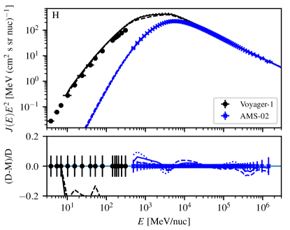
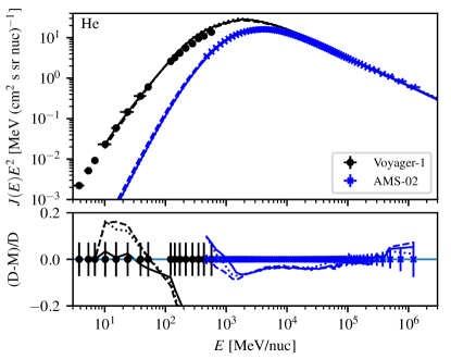
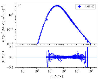
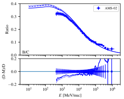
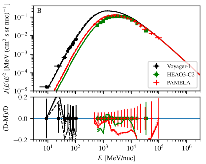
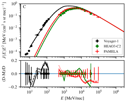
Figure 4.— GALPROP predictions calculated using the new 3D gas distributions and CR source density models compared with CR data: SA0 (solid curve), SA50 (dotted curve), and SA100 (dashed curve). Shown are CR species: protons (top left), helium (top right), $e^{-}$ (center left), boron over carbon ratio (center right), boron (bottom left), and carbon (bottom right). Bottom panel of each figure shows the fractional residuals.

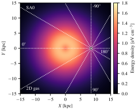
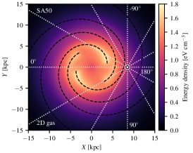
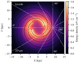
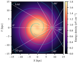
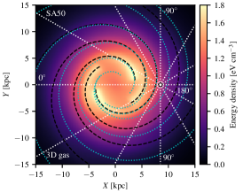
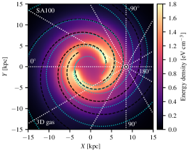
Figure 5.— Total CR energy density in the mid-plane of the Galaxy ($Z=0$) for SA0, SA50, and SA100 CR source distributions (left to right, respectively) with the 2D gas distribution on top and the 3D gas distribution at the bottom. The solar location is marked as a white point and the white dashed lines mark the longitude grid with 30^∘ step. The black dashed curves trace the positions of the spiral arms in the CR source distribution and the cyan dotted curves trace the spiral arms in the 3D gas distribution.

Comparison of the best-fit parameters of the models employing the 2D gas distributions with those using the new 3D gas distributions shows that there are significant changes in the normalization of the diffusion coefficient $D_{0}$ and its rigidity dependence $\delta$. There are also corresponding changes in the Alfvén velocity values $v_{A}$. Using the 3D gas distributions results in slower diffusion and weaker diffusive reacceleration. The main reason for this change in the parameter values is the lower local gas density for the 3D gas models. The average surface density of the combined interstellar gas within a few kpc of the Sun using the new 3D distributions is nearly a factor of 2 lower than that calculated using the 2D distributions. This is the region where most of the secondary Boron reaching the Earth is produced (Jóhannesson et al., 2016). The surface density, rather than central plane number density, is used for inter-comparison because the scale height of the CR diffusion zone is significantly larger than that of the gas and the surface density thus provides better estimate of total column density of the gas traversed by CRs. The difference in total surface density of about a factor of 2 agrees reasonably well with the factor of 2 change in $D_{0}$. In turn, slower diffusion results in weaker diffusive acceleration that is needed to reproduce the data.

The reason for this significant change in the local gas surface density between the distributions is two-fold. First the method for determination of the gas distribution using a student-t likelihood favors models that under-predict the data leaving residuals that can be absorbed by additional model components. This is evident from the positive residuals seen in Figure 3. Those cannot, however, explain a factor of 2 difference because the residuals around $l\sim 90^{\circ}$ and $l\sim-90^{\circ}$ are $\sim 40$% of the model and should therefore account for only about half of the difference. Another important difference between the gas distributions is that the older 2D distributions were derived assuming the Sun is located at 10 kpc from the GC (Gordon & Burton, 1976; Bronfman et al., 1988). These distributions have not been scaled to the IAU recommended value of $R_{\odot}=8.5$ kpc that is used for the GALPROP calculations. Convolving the old 2D gas distributions with GALGAS using the updated rotation curve and the updated solar location results in a significant over-prediction of the data. The 2D gas distributions for the newly released GALPROP version 56 have been re-scaled to the correct Sun-GC distance of $R_{\odot}=8.5$ kpc. The scaled 2D gas distributions provide a good agreement with the H i and CO data. Using the rescaled 2D gas distributions in GALPROP in a fit to the CR data results in $D_{0}=3.16\times 10^{28}$ cm²s^-1, which is about half-way between the results for the old 2D distributions and those obtained with the new 3D distributions. For compatibility with previous work and, in particular, the work by Porter et al. (2017) the calculations here do not use the corrected 2D gas distributions. GALPROP is not the only propagation code that uses these incorrectly scaled distributions, other codes that have incorporated the GALPROP analytic gas code and use it with $R_{\odot}=8.5$ kpc are also susceptible to the error.

The change in propagation parameters between the different CR source density models is small for both 2D and 3D gas distributions, but statistically significant. There is no obvious trend for most of the parameters. That is, the values for those of SA50 are not always between the values for SA0 and SA100. Note that the values of $v_{A}$ and $\delta$ determined here for the GALPROP 2D gas distributions differ from those obtained by Jóhannesson et al. (2016) and Cummings et al. (2016) because of the datasets employed. The larger value of the delta parameter comes from the reduced Alfvén speed obtained from the fits: higher Alfvén speeds result in a larger bump around $\sim$$1$ GeV in the B/C ratio than that required by the AMS-02 data used in this paper.

Figure 5 shows the total energy density of CRs in the Galactic plane for the 6 models considered in this paper. It illustrates how the gas and CR source distribution affects the final distribution of CRs in the Galaxy after propagation. The spiral arm structure of the CR source distribution is clearly visible. The visible width of the spiral arms is considerably larger than the input CR sources because of the diffusion. The change in diffusion parameters between the two gas distributions creates a visible and significant effect where the spiral arm features are distinctly sharper with the new gas distributions and smaller diffusion coefficient. The imprint on the gas distribution can also be seen for the SA0 CR source distribution where the enhanced density in the spiral arm causes faster cooling.

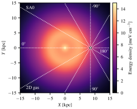
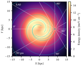
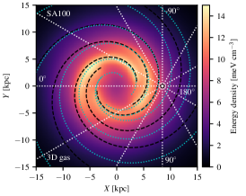
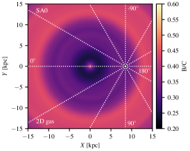
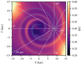
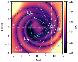
Figure 6.— Top row: CR energy density of secondary positrons in the mid-plane of the Galaxy for the SA0-2D gas (left), SA0-3D gas (center), and SA100-3D gas (right). Bottom row: B/C ratio at 10 GeV/nuc in the mid-plane of the Galaxy for same models. The lines and curves are the same as in Figure 5. The three labeled red dots with the white border in the bottom right panel mark locations for the CR spectra shown in Figure 7.

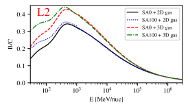
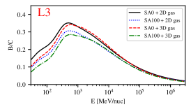
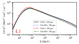
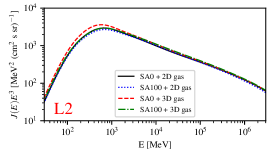
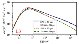
Figure 7.— Top row: B/C ratio for SA0-2D (black solid curve), SA100-2D (blue dotted curve), SA0-3D (red dashed curve), and SA100-3D (green dash-dotted curve) models at the positions marked by the red dots with the white border in Figure 6. Bottom row: positron spectrum plotted at those same locations for the same models. The red label in the panels corresponds to the appropriate dot location.

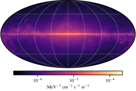
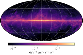
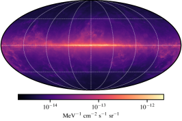
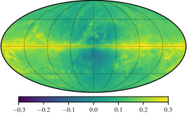
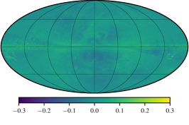
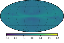
Figure 8.— Top row: total $\gamma$-ray intensity ($\pi^{0}$-decay, bremsstrahlung, and IC) at 30 MeV, 1.0 GeV, and 100 GeV energies (left to right, respectively) for SA0-2D gas reference case. Bottom row: fractional residuals from a comparison with SA0-3D gas ([SA0-3D – SA0-2D]/SA0-2D) at the same energies. The maps are in Galactic coordinates with $(l,b)=(0^{\circ},0^{\circ})$ at the centre with $l$ increasing to the left. The longitude meridians and latitude parallels have $45^{\circ}$ spacing.

The total energy density of CRs is dominated by protons with energies of about few GeV that are mostly primary in origin. The gas distribution only affects the primary CRs by changing the cooling and spallation rates and, therefore, has a minor impact on the total energy density. Secondary CRs are produced in interactions between primary CRs and interstellar gas, so the gas distribution has a much larger influence on CR secondaries and their spatial densities. This is illustrated in Figure 6, which shows the energy density of secondary positrons in the plane for selected models. The spiral arm distribution of the gas is clearly visible in the energy density distribution of the secondary particles, while the primary CR source distribution has only a relatively minor effect (Figure 5).

The different drivers for the spatial structure of the primary and secondary CRs result in non-trivial dependence of derived quantities, such as the secondary/primary ratios if the CR source and gas spatial densities are not aligned. This is illustrated in the B/C ratio shown in Figure 6. There is a clear reduction in the ratio along the spiral arm pattern of the CR source distribution (black dashed curves), while the ratio is seen to be larger along the spiral arm pattern of the gas distribution (cyan dotted curves). For the cases where the spiral arm patterns of both distributions aligns the effect of each almost cancels out. To further illustrate this point, the energy dependences of the B/C ratio at three selected locations in the Galaxy are shown in Figure 7. The locations are shown in the bottom right panel of Figure 6 and are chosen to be at the same Galactocentric distance $R_{\odot}$. The locations align with a spiral arm in the gas distributions (location L2), a spiral arm in the CR source distribution (location L3) or both (location L1). The exact CR and gas distributions can, therefore, have a large effect on the determination of the parameters of propagation models when calculating secondary production and the B/C ratio. The effect on the pure secondaries, such as secondary positrons shown in the bottom row of Figure 7 is dominated by the gas distributions because the distribution of primary sources have only a small effect.

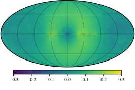
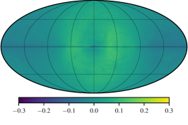
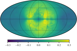
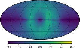
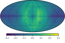
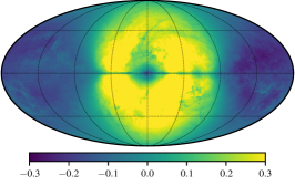
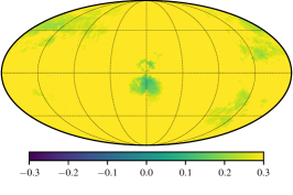
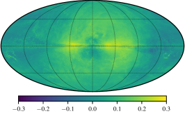
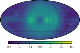
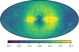
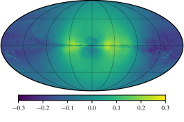
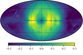
Figure 9.— Fractional residuals for the total $\gamma$-ray intensity ($\pi^{0}$-decay, Bremsstrahlung, and IC) at 30 MeV, 1.0 GeV, and 100 GeV energies (left to right, respectively) for SA50-2D gas, SA100-2D gas, SA50-3D gas, and SA100-3D gas (top to bottom, respectively) compared to SA0-2D gas reference model. The maps are in Galactic coordinates with $(l,b)=(0^{\circ},0^{\circ})$ at the center with $l$ increasing to the left. The longitude meridians and latitude parallels have $45^{\circ}$ spacing.

3.3. $\gamma$-ray maps

High-energy interstellar emissions are calculated using GALPROP for the SA0, SA50, and SA100 source density models (Section 3.2), and the standard 2D gas (Ackermann et al., 2012) and the new 3D gas model distributions. The standard 2D ISRF model (Ackermann et al., 2012) and the annular gas maps from Ajello et al. (2016) are used for all calculations. Because of the column density corrections described in Section 3.1, replacing the 2D gas distributions in GALPROP with the new 3D gas distributions will only affect the $\gamma$-ray skymaps through the change they have on the CR flux.

Calculations of the interstellar emission are made with the same spatial and kinetic energy grids that were used for tuning CR propagation parameters (Section 3.2). The $\gamma$-ray intensity maps are calculated for the energy range 30 MeV – 300 GeV using a logarithmic energy grid with 10 bins/decade spacing. Production of higher energy $\gamma$-rays involves interactions of CRs with energies above several TeV, where the assumption of a steady-state CR injection is less valid due to the stochastic nature of CR sources and fewer sources capable of accelerating particles to VHEs (Moskalenko et al., 2001; Bernard et al., 2013). Calculations of pion (and heavier mesons) production and decay are done using a parameterization by Kamae et al. (2006). Secondary $e^{\pm}$ produced in hadronic interactions are combined with primary electrons to calculate IC scattering. Their contribution to the interstellar emissions is important for energies $\lesssim 50$ MeV (Porter et al., 2008; Bouchet et al., 2011). All calculations of the IC emission use the anisotropic scattering cross section (Moskalenko & Strong, 2000a) that accounts for the full directional intensity distribution of the ISRF model.

The effects the two different gas distributions have on the total predicted $\gamma$-ray intensity are first explored. The differences between the model calculations in this paper are of the order of few tens of percent, which is much smaller than the variations in the calculated sky intensity that are few orders of magnitude, e.g., between low and high-latitude regions. Such differences between models are most usefully illustrated as relative differences compared to the reference case: SA0-2D gas. Modifications in the gas distributions used in GALPROP affect the propagation parameters and hence all three components of the interstellar emission: $\pi^{0}$-decay, Bremsstrahlung, and IC. Figure 8 shows a comparison between SA0-2D and SA0-3D model intensities. The top panels show the total intensity calculated in the SA0-2D model at 30 MeV, 1 GeV, and 100 GeV (left to right), while the bottom panels show the fractional difference between the two models, (SA0-3D – SA0-2D)/SA0-2D, for the same energies. The intensity at 30 MeV is dominated by Bremsstrahlung and IC emission from low-energy electrons with a large contribution from secondary electrons and positrons. At 1 GeV the intensity is dominated by the $\pi^{0}$-decay emission where 10 GeV particles contributing the most. The intensity at 100 GeV is still dominated by $\pi^{0}$-decay emission over most of the sky with IC emission contributing nearly equally in the inner Galaxy.

The most visible feature of the bottom ratio maps in Figure 8 is the positive residuals in the 30 MeV map, in particular for the local molecular clouds at low latitudes. This extra emission is almost entirely caused by increased Bremsstrahlung emission even though the models are tuned to the same electron data (Section 3.2). Because of the smaller number density of the gas in the 3D model and corresponding change in the propagation parameters, the local interstellar spectrum of electrons appears softer at low energies than for the case of the 2D gas model. Tuning to the same AMS-02 data thus requires a larger modulation potential. The softer interstellar spectrum of electrons leads to the enhanced Bremsstrahlung and IC emission compared to the reference case. The IC emission is, however, not as strongly affected because the average energy of the electrons generating most of the emission in this energy range is higher than for electrons producing Bremsstrahlung. Higher Bremsstrahlung $\gamma$-ray production also enhances the emissions from local gas that is distributed toward high-latitudes, but this is not visible in the ratio of the total intensity maps because IC emission dominates there. The effect is greatly reduced for GeV $\gamma$-rays, because Bremsstrahlung becomes subdominant at these energies.

Other effects visible at all energies are due to the difference in propagation parameters for the CR source and gas density combinations and the different spatial distribution of secondary CR particles in the Galaxy. The flux of secondary CRs in the outer Galaxy is smaller in the model using the 3D gas distributions compared to the reference case. The slower diffusion, however, results in more primary CR electrons in the outer Galaxy and less in the inner Galaxy compared to the reference case. This causes the bluish regions towards the inner Galaxy at intermediate latitudes where IC dominates over Bremsstrahlung and $\pi^{0}$-decay emission. The enhancement of the IC emission in the outer Galaxy is not visible in these total ratio maps because it is subdominant, particularly at 1 GeV. The decreased emission in the outer Galaxy, which shows as a sharp drop in the fractional residual maps at the annular gas map boundaries in the outer Galaxy, is a result of less Bremsstrahlung and $\pi^{0}$-decay emission in the outer Galaxy. Emissions from local clouds dominate the intensity in the outer Galactic plane, which explains why the ratio is slightly above 1 for the local clouds. The spiral arm structure of the 3D gas distributions is not visible in the fractional ratio maps because they affect the total $\gamma$-ray intensity by only a few percent, which is smaller than the effect caused by the change in propagation. Even though the effects of the spiral arm features are small in the total intensity the magnitude of the difference can be up to 15% for individual Galactocentric annular maps (not shown).

Comparisons of models with CR sources in the spiral arms, SA50 and SA100, are shown in Figure 9 as fractional residuals against the reference model. Shown are residuals for both the 2D and 3D gas distributions. The spiral arm contribution in the CR source distribution falls off more quickly with Galactic radius than the disk contribution. This causes reduced emission in the outer Galaxy for models with a higher fraction of sources in the spiral arms. The same effect also causes an increased flux of CRs in the inner Galaxy that produces an increased intensity towards the inner Galaxy, but the lack of sources at $R<3$ kpc in the spiral arm component results in a reduced intensity near the GC. This combination produces the doughnut-like shape in the residuals towards the inner Galaxy. The effect is enhanced for the CR electrons because they lose energy more quickly than nuclei and, therefore, do not travel very far from their sources. The enhancements around the spiral arm tangents are, therefore, mostly visible in Bremsstrahlung and IC emission components. These can be seen in 30 MeV and 100 GeV fractional residual maps, where one of these components or both are bright enough. Correspondingly, the tangents are least visible in the fractional residuals at 1 GeV where the $\pi^{0}$-decay component dominates.

The increased brightness of the 30 MeV map for the SA50-3D gas model is due to the larger value needed for the AMS-02 modulation potential to match the CR data (see Table 5). As discussed before there is considerable degeneracy between the determination of the heliospheric modulation and the low-energy CR intensities. Combined with non-linear CR propagation models and numerical uncertainties, this can lead to the minimizer having difficulties in finding the true best-fit parameters when fitting to CR data. This may explain why the values for the modulation potential differ so significantly between the three models using the 3D gas distribution. Fermi–LAT data can be used to further constrain the spectrum of CR electrons, but such analysis requires modeling outside the scope of this paper and is deferred to future work.

The effects of variations of the CR source distribution on the $\gamma$-ray intensity maps are fairly similar in cases of 3D and 2D gas distributions. There is a reduction in the intensity in the outer Galaxy and toward the GC while the intensity in the inner Galaxy increases. The details are, however, somewhat different. The slower diffusion combined with the same electron cooling rate leads to more CR electrons near their sources and fewer far from the plane. The doughnut like excess towards the inner Galaxy is thus more asymmetric with higher intensity near the plane. This is most visible at 100 GeV where the increased intensity for latitudes $|b|\gtrsim 30^{\circ}$ is suppressed compared to the same source models with the 2D gas distribution. This effect also enhances and sharpens the spiral arm tangent features for both IC and Bremsstrahlung. The CR nuclei are not as strongly affected because the change in the gas number density and hence the cooling and fragmentation rates compensate to some extent for the change in the diffusion coefficient.

4. Discussion

The 3D gas density models derived in this work employ only a few spatial distribution components, which are able to account for the main features of the interstellar gas with relatively few parameters. This enables the model fitting to be made within a reasonable time frame. Among the elements held constant for the tuning of the gas distribution models is the gas rotation field, which defines the conversion between distance and velocity. To test the effect of varying the rotation field a fit to the gas data was performed using a model with the rotation curve of Clemens (1985), but other components were kept the same. Using this rotation curve resulted in an overall worse fit of the data, as determined by the log-likelihood. Considerably more overlap between spiral arms was evident, and the features in the longitude–velocity diagram of the model did not match those in the data as well as the best-fit model determined above. The smooth disk also contained a larger fraction of the total mass of the model. The assumed velocity field is, therefore, very important for accurate determination of a 3D spatial density model for the interstellar gas.

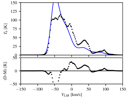
Figure 10.— The H i velocity spectrum in the direction of $(l,b)=(-50^{\circ},0^{\circ})$. Data are shown as black points with error bars smaller than the point size. The blue curve shows the model calculations. The residuals are shown at the bottom panel.

Inclusion of a detailed description for the non-cylindrical streaming motions into the models would add another level of complexity to the analysis and was not attempted in the present work. However, to test their effect a simplified sinusoidally varying radial component

$$v_{r}(\Theta)=v_{r,0}\sin(\Theta-\theta_{r,0})$$ (13)

was added to the cylindrical rotation with $v_{r,0}$ and $\theta_{r,0}$ as free parameters. The same model fitting procedure was then followed as for the H i and CO models described above with all components included. The likelihood improved with this additional component, but not by enough to warrant its inclusion into the final models. The improvement in the likelihood came almost entirely from a somewhat closer match to the data for the H i model. The total mass for the atomic and molecular gas density models increases with this modification, which is expected for an improved fit.

The total gas mass in the H i model increases to $6.0\times 10^{9}$ M_⊙ with almost all increase due to the spiral arms. The radial number density distributions of the disk and arms also become flatter, being nearly constant from 2 kpc to 15 kpc from the GC and varying only by $\sim$25% over the entire range. The gas mass in the CO model slightly increases to $0.74\times 10^{9}$ M_⊙, where most of the increase is due to the bulge/bar component. The radial density distribution of the CO disk/arm component is also flatter, having about 20% of the disk mass in the outer Galaxy compared to 5% without the velocity modifications.

The mophology of the spiral arms also changes: the pitch angles for all arms fall in between $12.0^{\circ}$ and $13.5^{\circ}$ with all starting points in the range 3.1–3.6 kpc. The spiral arms are thus more symmetric in their shapes. The arm densities for the CO model are still very asymmetric with both arm 1 and arm 2 set to zero by the fit to the CO data. In particular, arm 2 that has been identified with Sagittarius and Carina in the model still does not match the features in the CO data. The flaring parameter, $r_{z}$, increases and is now in better agreement with that determined by Kalberla & Dedes (2008). The warp changes slightly with all the warp-related parameters increasing more slowly with radius without changing its azimuthal dependence.

The resulting velocity field is broadly consistent with that found by Tchernyshyov & Peek (2017) and shown in their Figure 5. There are negative velocity corrections close to the GC and in the outer Galaxy for longitudes larger than $180^{\circ}$, while the corrections are positive in the outer Galaxy for longitudes smaller than $180^{\circ}$. The only large-scale feature they found that is not reproduced is the positive peculiar velocity around longitude $\sim 45^{\circ}$. The final value for $v_{r,0}$ was around 28 km s^-1, so the magnitude of the variations is also similar to that obtained by Tchernyshyov & Peek (2017). This shows that streaming motions are important to consider, but also that these simple modifications to the velocity field in combination with the geometrical model derived in this paper do not qualitatively change the final results. In particular, the effect on the CR propagation parameters is only minor.

The neutral hydrogen in the interstellar gas is not uniform. It is composed of, at least, three different phases that can be separated by their temperature: the stable cold, the stable warm and the unstable warm (Verschuur & Magnani, 1994). Observations have shown that each of these phases contain about one third of the total mass of the neutral hydrogen (Heiles & Troland, 2003). Different temperatures of these phases result in widely different broadening of the line emission profiles, ranging from few km s^-1 for the cold phase up to few tens of km s^-1 for the warm stable phase.

The average density of the gas in these phases is also different with the cold gas generally being about an order of magnitude denser than the warm gas. The single temperature analysis employed in this work uses the optically thin approximation that is appropriate only for the warm neutral medium and cannot be expected to capture all density structure of the neutral hydrogen. In particular, the cold component should exhibit smaller average line broadening than employed in this work. The spiral arm components are the densest parts of the H i model and are also likely to have a larger fraction of the cold medium than the more diffuse disk component, therefore, their line profiles are narrower than the disk line profiles.

Colder gas is also more likely to be optically thick. The gas number density in the structures consisting of the cold phase is thus under-predicted in this work because of both, the model inability to reproduce the observed narrow emission lines, and the optically thin assumption that over-predicts the line emissivity per hydrogen atom. An improved treatment that accounts for the multi-component neutral medium is necessary to simultaneously account for the cold and warm phases. The results of the current paper should be considered as providing an approximate lower bound to the true gas number density in the Galaxy.

Even though the models developed in this paper generally under-predict the data, there are a few exceptions. An example can be found in the H i longitude profiles shown in Figure 3. The model over-prediction toward the GC can be seen, though the number density in the H i model becomes nearly 0 at the GC (see Table 1 and Figure 1). The over-prediction is likely a consequence of using the optically thin approximation in Eq. (2). To test this hypothesis, the analysis was redone assuming a constant $T_{S}=150$ K throughout the Galaxy. This results in a lower brightness temperature toward the inner Galaxy despite the gas number density being non-zero and the total H i mass being $\sim 10$% higher than determined using the optically thin assumption. The reduced brightness is the result of absorption from foreground gas that has higher opacity in the model with lower $T_{S}$. The likelihood of the model with the lower $T_{S}$ value is, however, significantly lower. This simple modification may help data agreement in the direction toward the GC, but other regions then are not fitted very well.

The optically thin assumption may also affect the model-data agreement in other regions. In particular, near the Crux-Centaurus arm tangent at $l\approx-50^{\circ}$, the model significantly over-predicts the data. This is shown in the velocity spectra in the LOS towards $(l,b)=(-50^{\circ},0^{\circ})$ in Figure 10. Using $T_{S}\sim 110$ K, the peak of the $T_{S}$ distribution estimated by Strasser & Taylor (2004), would reduce the model prediction to agree well with the data in that direction. However, the assumption of a single value for $T_{S}$ over the entire Galaxy would unlikely result in a global improvement in the model-data agreement because of the non-linearity of the optical depth correction, Eq. (2). Instead, modeling $T_{S}$ variations throughout the Galaxy that takes into account observations of H i in absorption, where possible, may help.

The modifications of the $\gamma$-ray maps due to the implementation of the new 3D gas distributions can almost be entirely attributed to changes in the calculated CR flux. This is because the final maps are scaled with column densities determined from the line emission surveys for each LOS. Because of large uncertainties in the properties of the CR source distributions these changes may be compensated for, at least partially, by variations in the CR source distribution. This work has shown that changing the CR source distribution has a larger effect on the $\gamma$-ray maps than changing the gas distributions used by the propagation codes. The correlation between the gas distribution and CR source distribution does not mean, however, that using a more realistic gas distribution is unnecessary. On the contrary using the best available gas distribution is vital if attempting to use $\gamma$-ray observations to constrain the properties of CR sources and propagation.

The most popular method for determining the CR source distribution from $\gamma$-ray data is to use the annular maps created from the line emission surveys and assume the CRs illuminate the gas uniformly. This is a useful first approximation, but the calculations made in this paper show that implementation of the 3D distributions of CR sources and components of the interstellar medium can result in variations of tens of percent within a single annular map, which is far greater than the statistical uncertainty of current data that is less than one percent. Also, the annular maps may provide excellent resolution and details on the sky, but they suffer from poor distance resolution and near-far distance ambiguities. The 3D gas models are, therefore, necessary to accurately weight the CR flux within the region covered by the annular map. This is even more important if 3D source density distributions are used.

The SA0–2D model is based on the same assumption as the ^SL${}^{\rm Z}6^{\rm R}20^{\rm T}150^{\rm C}5$ model of Ackermann et al. (2012) and the Pulsars model of Ajello et al. (2016). It is interesting to compare the fractional residual maps in Figure 8 and Figure 9 to the fractional residual maps presented in these two earlier studies. In Figure 7 of Ackermann et al. (2012) there is a general trend of negative residuals for the latitudes ranges $5^{\circ}<|b|<15^{\circ}$ that corresponds to the reduction in IC emission at these latitudes when using the 3D gas distribution. This is also in agreement with the scaling factor for the ISRF in that work being less than 1 in their inner Galaxy region. There is also indication of asymmetry in the residuals along the plane with positive residuals at $l\sim 45^{\circ}$ and negative residuals at $l\sim-45^{\circ}$. A similar pattern is also seen the residuals in Figure 2 of Ajello et al. (2016). While none of the models in this work show this exact behavior it is not difficult to imagine modifications to the CR source distribution that could naturally account for such model asymmetries.

5. Summary

New 3D models for the large-scale distributions of atomic and molecular gas in the Galaxy have been developed. They are based on a combination of a limited number of geometric components with smoothly varying number density that enables the description of the observed large-scale structure: the warped disk, the central bulge/bar, and the 4 major spiral arms. The parameters of model components have been tuned to match the LAB 21-cm line emission survey (Kalberla et al., 2005) and the CfA composite CO survey (Dame et al., 2001). The best-fit parameters and resulting models agree very well with previous work, but it is the first time that they are presented together within a single consistent framework. To study the effects of variations in the gas and source distributions on CR propagation parameters they are incorporated into the GALPROP CR propagation code. The new gas density models significantly affect the best-fit values of CR propagation parameters determined from the fits to local CR data. The parameter values depend on both the CR source density distribution and the gas density models and will have to be re-evaluated as better models are constructed.

The effects that three different CR source density models with different injection rates in the smooth disk and spiral arms components have on the $\gamma$-ray intensity skymaps have also been investigated. The combined 3D CR source and gas density models produce non-trivial features in the large-scale $\gamma$-ray residual sky maps that can be compared with those obtained from the prior analysis of the interstellar $\gamma$-ray emissions observed by the Fermi–LAT. Elements of the 3D models provide an explanation for residual features previously obtained from analysis of $\gamma$-ray data using the 2D axisymmetric models.

Appendix A GALGAS description

The GALGAS code is designed to calculate line-emission profiles from the Galaxy for user-provided gas density and velocity distributions. Efficient evaluation of a likelihood function many times is necessary for the model-data fits. The code is written in C++ and is parallelized using OpenMP for CPUs and OpenCL for execution on GPUs (the code operates using both if available on a given system). The code calculates the line-emission profile on a HEALPix grid. The emission of each pixel is uniform and its value determined from the LOS going through the center of the pixel. Each LOS profile is binned in the same way linearly in velocity. For each pixel the code first calculates the transformation from distance to velocity for a given velocity field $\boldsymbol{v}(X,Y,Z)$ by calculating the difference in velocity between the location of the Sun and the location along the LOS, projected onto the LOS. The code steps through the LOS beginning from the Sun and finding the distance points corresponding to the boundaries of the velocity bins. A coarse search is initially performed using a step size based on the gradient of the projected velocity, then the distances are further refined using a bisection search. A maximum of 20 bisection steps are taken for each point. More efficient search methods were found to be less stable than the bisection method and, therefore, not considered. The code currently steps along the LOS until it reaches a distance of 100 kpc. Even though each LOS is independent, this part of the code executes only on the CPU because the branching for the current algorithm is inefficient for execution on the GPU. The results from the transformation calculations are cached internally and only recalculated as needed if the parameters of the velocity field change.

Once the transformation from velocity to distance has been established, the actual LOS integration is performed on the GPU. Each distance bin is independently integrated using 61 point Gauss-Konrod integration rule. The integrator does not handle radiative transfer, so each bin is assumed to have constant average optical depth for absorption. For CO, the line emission is assumed to be optically thin and therefore linearly related to the density, while for H i Eq. (2) is used to estimate the line intensity. The $T_{S}$ is calculated as the average of a given $T_{S}(X,Y,Z)$ distribution over the distance bin. While the integration over the LOS is performed on the GPU, the transformation from the distance bin grid to the velocity grid is calculated on the CPU. The model is then smoothed in velocity with a Gaussian kernel to account for thermal and turbulent motions of the gas. The width of the kernel is parameterized by velocity and then internally binned to match the specified velocity grid. The actual convolution with the kernel is performed on the CPU. Profiling of the code revealed that performing this on the GPU would result in small gains only.

The model-data comparison is done using a student-t likelihood with a user specified degrees of freedom. The input data can be either a HEALPix cube or a CAR projected cube. The code automatically rebins the CAR cubes into the HEALPix format and the user specified velocity binning. It can also handle data that are split into several longitude bins, such as the LAB split data format. Simple filters can be specified as rectangular regions in longitude, latitude, and velocity. These are useful to filter out high-velocity data and Local Group galaxies from the H i data. The filtered and rebinned data can be cached for future use so rebinning does not happen each time a new fit is performed. The likelihood calculation is made on the CPU (execution on the GPU for this part does not increase the performance of the code significantly).

The model is defined using an XML based model format. The density models use the galstruct library from the GALTOOLSLIB package distributed with the GALPROP code. Each density model is composed of different components or building blocks that is each derived from a base C++ class in the galstruct library. Adding a new component simply requires writing a new class that defines the functional form and its parameters. Once the class is registered with an identification string in the code it can be used in the XML input file and given a unique name. The velocity field model is based on a similar concept and is composed of different components as well. The initial values and boundaries of the fitted parameters are specified in the XML file. Upper and lower boundaries are set independently and they can be turned off completely. Parameters can also be fixed to their initial values. All parameters have a name that is determined from the given component name and the default name of the parameter. This way the same component (e.g., a spiral arm) can be included many times in the model with each instance having its own individual parameters. This default name of parameters can be overridden with a special name tag. By assigning the same name to two parameters they become linked in the fitting procedure and take the same value.

Once the fitting procedure is done and the best-fit parameters have been derived, the code outputs the model configurations as XML files with updated values. The code also outputs the parameter values along with their uncertainties as a text file. By default, the code stores the best-fit model and the data-model residual as HEALPix cubes. The code can also calculate the surface density, the first moment of the vertical density distribution (Eq. [12]), the vertical thickness of the density distribution using the definition from Levine et al. (2006), and the longitude-velocity diagram. The code is configured with a simple text based parameter file where all the input and options are defined.

References

- Abdo et al. (2009) Abdo, A. A., et al. 2009, Physical Review Letters, 103, 251101
- Abdo et al. (2010) —. 2010, ApJ, 710, 133
- Ackermann et al. (2011) Ackermann, M., et al. 2011, ApJ, 726, 81
- Ackermann et al. (2012) —. 2012, ApJ, 750, 3
- Adriani et al. (2009) Adriani, O., et al. 2009, Nature, 458, 607
- Adriani et al. (2014) —. 2014, ApJ, 791, 93
- Aguilar et al. (2013) Aguilar, M., et al. 2013, Physical Review Letters, 110, 141102
- Aguilar et al. (2014) —. 2014, Physical Review Letters, 113, 121102
- Aguilar et al. (2015a) —. 2015a, Physical Review Letters, 115, 211101
- Aguilar et al. (2015b) —. 2015b, Physical Review Letters, 114, 171103
- Aguilar et al. (2016) —. 2016, Physical Review Letters, 117, 231102
- Ajello et al. (2016) Ajello, M., et al. 2016, ApJ, 819, 44
- Bernard et al. (2013) Bernard, G., et al. 2013, A&A, 555, A48
- Bohlin et al. (1978) Bohlin, R. C., Savage, B. D., & Drake, J. F. 1978, ApJ, 224, 132
- Bolatto et al. (2013) Bolatto, A. D., Wolfire, M., & Leroy, A. K. 2013, ARA&A, 51, 207
- Boschini et al. (2017) Boschini, M. J., et al. 2017, ApJ, 840, 115
- Boschini et al. (2018) Boschini, M. J., et al. 2018, eprint arXiv:1801.04059
- Bouchet et al. (2011) Bouchet, L., et al. 2011, ApJ, 739, 29
- Bronfman et al. (1988) Bronfman, L., Cohen, R. S., Alvarez, H., May, J., & Thaddeus, P. 1988, ApJ, 324, 248
- Burton (1988) Burton, W. B. 1988, The structure of our Galaxy derived from observations of neutral hydrogen, ed. K. I. Kellermann & G. L. Verschuur, 295–358
- Chemin et al. (2015) Chemin, L., Renaud, F., & Soubiran, C. 2015, A&A, 578, A14
- Clemens (1985) Clemens, D. P. 1985, ApJ, 295, 422
- Cummings et al. (2016) Cummings, A. C., et al. 2016, ApJ, 831, 18
- Dame (2011) Dame, T. M. 2011, eprint arXiv:1101.1499
- Dame et al. (2001) Dame, T. M., Hartmann, D., & Thaddeus, P. 2001, ApJ, 547, 792
- Dame & Thaddeus (2011) Dame, T. M., & Thaddeus, P. 2011, ApJ, 734, L24
- Dickey & Lockman (1990) Dickey, J. M., & Lockman, F. J. 1990, ARA&A, 28, 215
- Dickey et al. (2009) Dickey, J. M., et al. 2009, ApJ, 693, 1250
- Engelmann et al. (1990) Engelmann, J. J., Ferrando, P., Soutoul, A., Goret, P., & Juliusson, E. 1990, A&A, 233, 96
- Ferrière et al. (2007) Ferrière, K., Gillard, W., & Jean, P. 2007, A&A, 467, 611
- Ferrière (2001) Ferrière, K. M. 2001, Reviews of Modern Physics, 73, 1031
- Florinski et al. (2003) Florinski, V., Zank, G. P., & Pogorelov, N. V. 2003, Journal of Geophysical Research (Space Physics), 108
- Freudenreich (1998) Freudenreich, H. T. 1998, ApJ, 492, 495
- Gleeson & Axford (1968) Gleeson, L. J., & Axford, W. I. 1968, ApJ, 154, 1011
- Glover & Mac Low (2011) Glover, S. C. O., & Mac Low, M.-M. 2011, MNRAS, 412, 337
- Gordon & Burton (1976) Gordon, M. A., & Burton, W. B. 1976, ApJ, 208, 346
- Górski et al. (2005) Górski, K. M., et al. 2005, ApJ, 622, 759
- Heiles & Troland (2003) Heiles, C., & Troland, T. H. 2003, ApJS, 145, 329
- Hunter et al. (1997) Hunter, S. D., et al. 1997, ApJ, 481, 205
- Johannesson et al. (2015) Johannesson, G., Moskalenko, I. V., Orlando, E., Porter, T., & Strong, A. 2015, in International Cosmic Ray Conference, Vol. 34, 34th International Cosmic Ray Conference (ICRC2015), 517
- Johannesson et al. (2013) Johannesson, G., Moskalenko, I. V., & Porter, T. 2013, Br. J. of Phys., ICRC2013, 0913
- Jóhannesson et al. (2016) Jóhannesson, G., et al. 2016, ApJ, 824, 16
- Kalberla et al. (2005) Kalberla, P. M. W., et al. 2005, A&A, 440, 775
- Kalberla & Dedes (2008) Kalberla, P. M. W., & Dedes, L. 2008, A&A, 487, 951
- Kalberla et al. (2007) Kalberla, P. M. W., Dedes, L., Kerp, J., & Haud, U. 2007, A&A, 469, 511
- Kalberla & Kerp (2009) Kalberla, P. M. W., & Kerp, J. 2009, ARA&A, 47, 27
- Kamae et al. (2006) Kamae, T., Karlsson, N., Mizuno, T., Abe, T., & Koi, T. 2006, ApJ, 647, 692
- Kissmann et al. (2017) Kissmann, R., Niederwanger, F., Reimer, O., & Strong, A. W. 2017, in American Institute of Physics Conference Series, Vol. 1792, 6th International Symposium on High Energy Gamma-Ray Astronomy, 070011
- Kulkarni & Heiles (1988) Kulkarni, S. R., & Heiles, C. 1988, Neutral hydrogen and the diffuse interstellar medium, ed. K. I. Kellermann & G. L. Verschuur, 95–153
- Langner et al. (2006) Langner, U. W., Potgieter, M. S., Fichtner, H., & Borrmann, T. 2006, ApJ, 640, 1119
- Lebrun & Paul (1979) Lebrun, F., & Paul, J. A. 1979, International Cosmic Ray Conference, 12, 13
- Lebrun et al. (1983) Lebrun, F., et al. 1983, ApJ, 274, 231
- Levine et al. (2006) Levine, E. S., Blitz, L., & Heiles, C. 2006, ApJ, 643, 881
- López-Corredoira et al. (2007) López-Corredoira, M., et al. 2007, AJ, 133, 154
- Marasco et al. (2017) Marasco, A., Fraternali, F., van der Hulst, J. M., & Oosterloo, T. 2017, A&A, 607, A106
- Moskalenko et al. (2001) Moskalenko, I. V., Mashnik, S. G., & Strong, A. W. 2001, International Cosmic Ray Conference, 5, 1836
- Moskalenko et al. (2006) Moskalenko, I. V., Porter, T. A., & Strong, A. W. 2006, ApJ, 640, L155
- Moskalenko & Strong (1998) Moskalenko, I. V., & Strong, A. W. 1998, ApJ, 493, 694
- Moskalenko & Strong (2000a) —. 2000a, ApJ, 528, 357
- Moskalenko & Strong (2000b) —. 2000b, Ap&SS, 272, 247
- Moskalenko et al. (2005) Moskalenko, I. V., Strong, A. W., & Mashnik, S. G. 2005, in American Institute of Physics Conference Series, Vol. 769, International Conference on Nuclear Data for Science and Technology, ed. R. C. Haight, M. B. Chadwick, T. Kawano, & P. Talou, 1612–1617
- Nakanishi & Sofue (2003) Nakanishi, H., & Sofue, Y. 2003, PASJ, 55, 191
- Nakanishi & Sofue (2016) —. 2016, PASJ, 68, 5
- Nava et al. (2017) Nava, L., Benyamin, D., Piran, T., & Shaviv, N. J. 2017, MNRAS, 466, 3674
- Niederwanger et al. (2017) Niederwanger, F., Reimer, O., Kissmann, R., & Tuffs, R. 2017, in American Institute of Physics Conference Series, Vol. 1792, 6th International Symposium on High Energy Gamma-Ray Astronomy, 070015
- Orlando & Strong (2013) Orlando, E., & Strong, A. 2013, MNRAS, 436, 2127
- Parker (1965) Parker, E. N. 1965, Planet. Space Sci., 13, 9
- Planck Collaboration et al. (2015) Planck Collaboration et al. 2015, A&A, 582, A31
- Pohl et al. (2008) Pohl, M., Englmaier, P., & Bissantz, N. 2008, ApJ, 677, 283
- Porter et al. (2017) Porter, T. A., Jóhannesson, G., & Moskalenko, I. V. 2017, ApJ, 846, 67
- Porter et al. (2008) Porter, T. A., Moskalenko, I. V., Strong, A. W., Orlando, E., & Bouchet, L. 2008, ApJ, 682, 400
- Potgieter & Langner (2004) Potgieter, M., & Langner, U. 2004, Annales Geophysicae, 22, 3729
- Robitaille et al. (2012) Robitaille, T. P., et al. 2012, A&A, 545, A39
- Sanna et al. (2017) Sanna, A., Reid, M. J., Dame, T. M., Menten, K. M., & Brunthaler, A. 2017, Science, 358, 227
- Schlafly et al. (2017) Schlafly, E. F., Peek, J. E. G., Finkbeiner, D. P., & Green, G. M. 2017, ApJ, 838, 36
- Schlafly et al. (2014) Schlafly, E. F., et al. 2014, ApJ, 789, 15
- Schlegel et al. (1998) Schlegel, D. J., Finkbeiner, D. P., & Davis, M. 1998, ApJ, 500, 525
- Shaviv et al. (2009) Shaviv, N. J., Nakar, E., & Piran, T. 2009, Physical Review Letters, 103, 111302
- Sofue et al. (2009) Sofue, Y., Honma, M., & Omodaka, T. 2009, PASJ, 61, 227
- Sofue (2017) Sofue, Y. 2017, MNRAS, 468, 4030
- Strasser & Taylor (2004) Strasser, S., & Taylor, A. R. 2004, ApJ, 603, 560
- Strong & Moskalenko (1998) Strong, A. W., & Moskalenko, I. V. 1998, ApJ, 509, 212
- Strong et al. (2007) Strong, A. W., Moskalenko, I. V., & Ptuskin, V. S. 2007, Annual Review of Nuclear and Particle Science, 57, 285
- Strong et al. (2000) Strong, A. W., Moskalenko, I. V., & Reimer, O. 2000, ApJ, 537, 763
- Tchernyshyov & Peek (2017) Tchernyshyov, K., & Peek, J. E. G. 2017, AJ, 153, 8
- Vallée (2014) Vallée, J. P. 2014, ApJS, 215, 1
- Vallée (2016) —. 2016, AJ, 151, 55
- Vallée (2017) —. 2017, NewAR, 79, 49
- Verschuur & Magnani (1994) Verschuur, G. L., & Magnani, L. 1994, AJ, 107, 287
- Vladimirov et al. (2011) Vladimirov, A. E., et al. 2011, Computer Physics Communications, 182, 1156
- Yusifov & Küçük (2004) Yusifov, I., & Küçük, I. 2004, A&A, 422, 545