The Durham Adaptive Optics Simulation Platform (DASP): Current status

Abstract

The Durham Adaptive Optics Simulation Platform (DASP) is a Monte-Carlo modelling tool used for the simulation of astronomical and solar adaptive optics systems. In recent years, this tool has been used to predict the expected performance of the forthcoming extremely large telescope adaptive optics systems, and has seen the addition of several modules with new features, including Fresnel optics propagation and extended object wavefront sensing. Here, we provide an overview of the features of DASP and the situations in which it can be used. Additionally, the user tools for configuration and control are described.

The Durham adaptive optics (AO) simulation platform (DASP) has been under development since the early 1990s. Its current framework was established in 2006 to meet the challenges of modelling the forthcoming extremely large telescopes, with primary mirror diameters of over 20 m. Since 2006, DASP has been regularly developed to improve computational performance, increase simulation fidelity, and expand the number of features that can be modelled. It uses a modular design, allowing new developments and algorithms to be added whilst maintaining compatibility. DASP is developed primarily in Python and C, and uses pthreads and MPI for parallelization enabling modelling of the largest proposed telescopes on reasonable timescales.

1 Motivation and significance

The Earth’s atmosphere has a perturbing effect on incident starlight, meaning that the effective spatial resolution of large telescopes (typically anything larger than 20 cm diameter) is limited. By using AO systems, the distorted wavefronts of incident light can be measured and have a correction applied so that the effective resolution is improved, thus enabling scientific observations to be made. Designing an AO system to meet complex scientific requirements is an involved process, and modelling of the system performance is necessary. Additionally, investigation of new algorithms, techniques and concepts also requires verification by simulation.

1.1 Scientific contribution of DASP

DASP was developed to meet the needs of AO system designers, and has previously been used to model the expected performance of several of the forthcoming Extremely Large Telescope (ELT) instruments, including MOSAIC [1, 2], MAORY [3] and HIRES. Recent developments have also introduced an extended object (wide field-of-view) wavefront sensor module, enabling DASP to be used for the modelling of solar AO systems (e.g. European Solar Telescope [4]). Additionally, existing instruments have also been modelled to demonstrate that proposed novel techniques can improve the AO system performance [5, 6].

DASP enables AO system designers to explore the large parameter spaces associated with AO system development, allowing system design trade-offs to be made in an informed manner, with typical parameters including AO system order, number of guide stars, and wavefront sensor pixel scale. DASP is used to design and optimize new AO systems, and to verify performance of existing systems. DASP can be a crucial tool for understanding the AO error budget, allowing cost-effective decisions to be made about the design optimizations that can be performed to allow a given design to meet its required performance targets.

DASP has seen adoption within the AO community, and is now used for forthcoming ELT instruments [3, 7], for the 10.4 m Gran Telescopio Canarias, the Kunlun Dark Universe Survey Telescope [8], the Chinese 2.16 m telescope [9] and for the proposed 12 m Chinese Large Optical Telescope.

1.2 Using DASP

DASP can be operated on any Linux computer, and also under the OS-X operating system. Once installed, the user will typically generate a new simulation configuration using the daspbuilder tool, which allows the user to select a number of configuration options covering most AO configurations, including single conjugate AO (SCAO), multi-conjugate adaptive optics (MCAO), ground layer AO (GLAO), laser tomographic AO (LTAO) and multi-object AO (MOAO). This generates the necessary configuration files, which can then be edited by the user. Alternatively, for more complex simulations, a daspsetup tool can be used to graphically design an AO system. This simulation is then executed to model AO performance. A further description of DASP usage is given in Section 3

1.3 Other AO simulations

There are a number of other Monte Carlo AO simulation tools freely available to the community, including YAO [10], CAOS [11], SOAPY [12], MAOS [13] and OOMAO [14]. OCTOPUS [15] is another Monte Carlo AO simulation tool, which is available from the European Southern Observatory upon request. However, none of these offer the combined performance and extended object wavefront sensing capabilities of DASP. In addition, a number of analytical modelling tools also exist, including PAOLA [16] and CIBOLA [17], though these tools are used for rapid prototyping and do not offer high fidelity.

2 Software description

DASP is comprised of a number of science modules, which model discrete parts of an AO system. These include wavefront sensors (including Shack-Hartmann and Pyramid sensors), deformable mirrors (including zonal and modal), atmospheric models, wavefront reconstruction modules, and astronomical object models. This modular design means that it is also possible for the user to add modules which can then be used during a simulation (for example, another wavefront sensor type). These science modules are linked together to represent the flow of information through the AO system, as shown in Fig. 1.

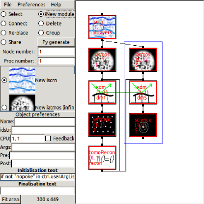
Figure 1: A screenshot of the daspsetup tool, showing the links between different science modules that create a simulation. This tool can be used to configure an initial simulation, which is then executed from the command line. Configuration of an AO simulation can be complicated when parallelization across multiple computing nodes is required, and the graphical tool simplifies this task.

DASP also contains a number of utility modules, which are used by the science modules, containing the necessary algorithms required by the simulation. User tools are also included, to analyse and display results, to communicate with running simulations, and to configure initial simulations. DASP offers good performance on laptops (for simulation of smaller scale systems, typically up to 10 m class diameter telescopes); and also HPC facilities for ELT modelling. Inter-node communication is based on the Message Passing Interface (MPI).

Once a simulation has been configured, it is run from the command line. After a set number of iterations (typically several thousand, depending on AO system type), the simulation then finishes, providing the user with AO performance metrics. Each iteration represents one simulation time-step, typically set by the integration time of wavefront sensors, of order 1 ms. It is usually necessary to model tens of seconds of real time in order to ensure that results are statistically valid. The simulation will typically run between 10–1000 times slower than real-time, depending on scale and complexity, though a simple system on a small (4 m) telescope can operate faster than real-time.

Using computationally efficient code allows large AO-related parameter spaces to be explored within reasonable timescales. For example, a typical ELT-scale wide-field AO simulation can be completed within about 12 hours on a single server, where previously this would have taken many days to complete. This includes the required system calibrations (e.g. interaction matrix generation and reference slope computation), for a system with 6 laser guide stars each with $80\times 80$ sub-apertures and a control matrix of size 10 GB, with sufficient temporal averaging to smooth the atmospheric turbulence effect (approximately 1 minute of AO system time).

Top level modules are written in Python, which allows rapid development of new algorithms and modules, enabling users to tailor DASP for their own use. While a simulation is running, it can be queried and modified using both command line and graphical tools, useful for when initially configuring a simulation. It also provides a way of rapidly determining stability conditions for an AO simulation before further extensive parameter space exploration.

2.1 Software Architecture

The DASP top-level directory structure separates the simulation into logical components:

• base/ containing simulation glue modules with no scientific component.

• cmod/ containing C code used to accelerate the simulation.

• docs/ containing documentation (including auto-generated API and user documentation).

• gui/ containing graphical user interfaces for simulation creation and control.

• science/ containing simulation science modules which represent a discrete part of an AO system.

• util/ containing utility modules with algorithms required by the simulation, which can also be used from a Python terminal by the user.

The science modules are used to form the structure of a simulation, and represent physical components. These all inherit from a base object providing a number of virtual methods to be inherited, which are called during initialisation and for every iteration of the running simulation. The science modules can also import components from the util/ and cmod/ directories, which provide necessary algorithms and improved computational performance. The base directory also contains glue modules, for example to handle MPI connection and modules without scientific content, such as First In First Out (FIFO) buffers. Fig. 2 provides an overview of the relationship between DASP components.

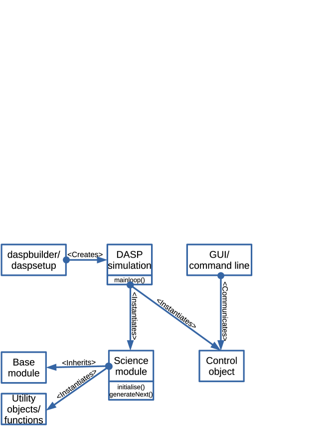
Figure 2: An overview of the DASP architecture, showing simulation science modules and their relationship with other DASP components.

A main DASP control object is instantiated, parses command line arguments and loads the specified configuration files. This object has a main control loop method, which is passed a list of instantiated base and science objects. These are then iterated over, calling the methods to compute the next iteration for each object.

2.1.1 Interaction and control

The control object also includes a communication thread which is used to allow external (user) connections to the running simulation. These connections can then be used to query and modify internal state, for example to alter the loop gain factor, pause the simulation, or to extract the current instantaneous AO system performance. This means that DASP can be used remotely on server computers, and that multiple simulations can be executed simultaneously, allowing the user to interact and connect to several simultaneously executing (independent) simulations. This allows a parameter space to be explored more rapidly. Additionally, multiple users can connect to a simulation simultaneously, to allow interaction and knowledge sharing.

2.2 Configuration

A DASP simulation structure is stored as an XML file, describing the links between the different science modules, and relevant multi-processor information (for example, on which process different science modules should be run, in the case of a multi-node simulation). This XML file is created using daspbuilder (command line) or daspsetup (graphical), and is then automatically parsed to generate a Python script.

A DASP simulation also requires one or more Python-based parameter files, which specify relevant parameters, dimension the system, and determine the outputs to be produced. The parameter file names are passed as command line parameters. The use of Python allows dynamic calculation of variables before execution, e.g. automated loading of external data files, and parsing of contents without requiring additional software tools.

2.3 Software Functionalities

The functionality of DASP is provided by the science modules. These include:

• Atmospheric phase screen generation: The atmosphere is modelled as a number of thin perturbing layers, which modify incident wavefront phase. A zonal extrusion technique is used [18] allowing screens of infinite length to be produced.

• Pupil phase generation: The perturbing phase introduced along a specified line of sight are identified and summed to give the perturbing phase at the telescope pupil, for this particular direction. Within DASP, both geometric ray tracing and Fresnel propagation can be used. Ray tracing is more computationally efficient and is the default option, though where high fidelity is important (e.g. photometry) Fresnel propagation should be selected, as scintillation effects are included.

• Deformable mirrors: A deformable mirror is a key component in an AO system, used to mitigate the turbulent phase, with a surface shape that is commanded by the AO control system to match the predicted wavefront phase perturbation as closely as possible. Both modal and zonal deformable mirror (DM) models are available. Zonal DM models include influence function and interpolated DMs (with spline interpolation between actuators to create the DM surface). An AO system may contain multiple DMs. A magic DM is also available, which corrects wavefront phase up to a set modal order without requiring a wavefront sensor.

• Wavefront sensor and centroider: A wavefront sensor is used to estimate the perturbing wavefront phase along a particular line of sight, in the direction of a guide star. Within DASP, Shack-Hartmann and Pyramid sensors can be used, and include aspects such as noise, pixel scale, thresholding and various image processing techniques. The wavefront gradients are estimated by the centroiding component, which can use a number of algorithms, including centre of gravity or correlation.

• Reconstructor: A wavefront reconstructor module is responsible for conversion between wavefront gradient measurements to DM shape. Multiple reconstructor algorithms are available, including dense matrix multiplication (including least squares and minimum variance approaches), sparse matrix multiplication using a de-densified control matrix (as studied in [19]), conjugate gradient solvers with preconditioning, and algorithmic reconstructors, e.g. the Hierarchical Wavefront Reconstructor (HWR) [20].

• Point spread function (PSF) generation: The point spread function (PSF) provides an instantaneous and long term (integrated) performance metric along a given line of sight, and is essential for diagnosing AO system capabilities.

• Extended object (wide-field) imaging and wavefront sensing: Most AO simulations consider a single line of sight for each wavefront sensor or PSF. However, DASP contains an extended object module which is able to consider directions within a set field of view simultaneously, enabling high fidelity modelling of solar AO systems, and those with extended laser guide star (LGS) spots.

• Real-time simulation: DASP contains a module which allows linkage to a real-time control system, the Durham AO Real-time Controller (DARC) [21, 22]. This therefore allows on-sky systems to be modelled, and algorithms within a real-time control system tested and developed, significantly reducing on-sky commissioning time. This hardware-in-the-loop capability is crucial for the forthcoming ELTs.

Additionally, the utility library also provides useful AO-related functions, including Zernike mode generation, pixel scale computation, point spread function (PSF) generation, etc.

2.4 Parsing results

Running a large number of simulations will generate a significant volume of performance data. Therefore DASP includes tools to allow the user to parse these data and extract relevant parameters into formats that can be used for further processing, analysis and display.

3 Illustrative Examples

DASP provides the ability to flexibly create high fidelity simulations of AO systems. Fig. 3 shows a simulated solar AO wavefront sensor, demonstrating the extended object wavefront sensing capability of DASP. A video of this wavefront sensor is also available from SoftwareX. A closed loop solar SCAO simulation is presented in A. First, the relevant modules are imported and simulation initialisation is performed, including instructions to perform initial calibrations (as with a real AO system). The science modules are then instantiated, and finally the main loop is entered.

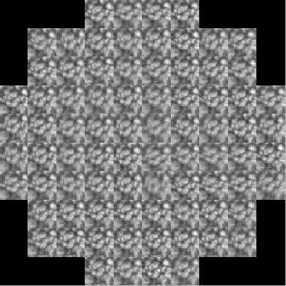
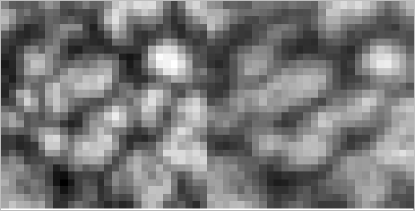
Figure 3: A simulated solar wavefront sensor image showing different atmospheric distortion across each sub-aperture. Two neighbouring sub-apertures are also shown in close-up, showing the relative distortion between them.

This code (along with the associated parameter file) will then generate an output file which contains PSF information such as the Strehl ratio, FWHM, ensquared energy, PSF diameter enclosing 50% of energy and rms wavefront error. The PSF itself can also be saved.

3.1 Hardware-in-the-loop example

As discussed previously, DASP can be linked with an AO real-time control system to provide a hardware-in-the-loop simulation capability. Fig. 4 shows the simulation configuration that is used with the CANARY AO instrument [23], and is an illustrative example of how DASP can be used in real-world situations to significantly reduce on-sky commissioning time [6]. In this case, DASP is used to model the atmosphere, telescope, and AO system optics, providing input to the CANARY real-time control system, and updating the model in response to real-time control system outputs.

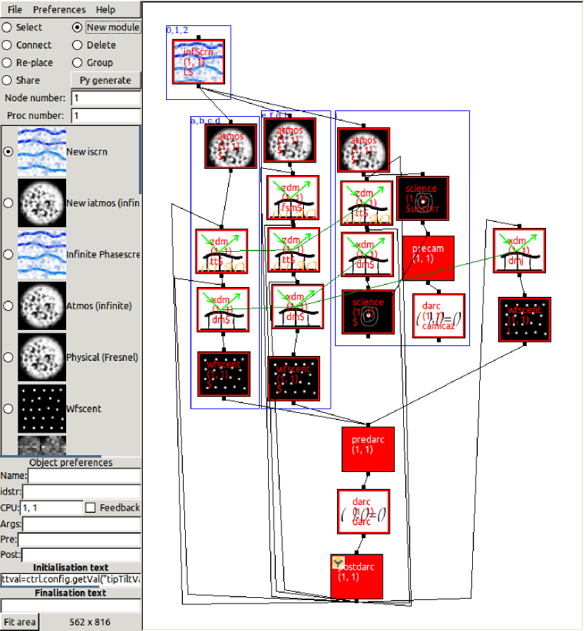
Figure 4: A figure showing the configuration of a hardware-in-the-loop simulation used with the CANARY AO instrument to reduce on-sky commissioning time. This figure is a screen-shot of the daspsetup tool and shows how a complex real-world simulation can be configured. The flexibility provided by DASP also leaves room for future expansion. Within this figure, one of the modules represents a link to (and from) a real-time control system.

4 Conclusions

DASP is a modular and flexible Monte-Carlo simulation tool for AO systems. It offers high fidelity modelling with good computational performance. DASP is suitable for use at forthcoming extremely large telescope scales, yet also offers the ability to rapidly prototype and test new algorithms and concepts. DASP has been used for simulation of both existing and forthcoming AO systems, and has been verified against other AO simulation codes [19].

Appendix A Solar AO system code listing

A code listing for a solar SCAO simulation.

⬇

import science.iscrn

import science.xinterp_dm

import science.wideField

import science.wfscent

import science.tomoRecon

import science.iatmos

import science.science

import util.Ctrl

#Initialisation

ctrl=util.Ctrl.Ctrl(globals=globals())

ctrl.doInitialOpenLoop(startiter=0)

ctrl.initialCommand("wf.control[’cal_source’]=1",freq=-1,startiter=0)

ctrl.initialCommand("wf.control[’cal_source’]=0",freq=-1,startiter=1)

#Obtain correlation reference images

ctrl.initialCommand("c.newCorrRef();print ’Done new corr ref’",freq=-1,startiter=1)

#Produce an interaction matrix

ctrl.doInitialPokeThenRun(startiter=2)

#instantiation of science modules:

#Phase screens

iscrn=science.iscrn.iscrn(None,ctrl.config,idstr="allLayers")

#Summed phase along a given direction

iatmos=science.iatmos.iatmos({"allLayers":iscrn},ctrl.config,idstr="b")

#Wide-field DM (for the wavefront sensor)

dm=science.xinterp_dm.dm(None,ctrl.config,idstr="dma")

#Narrow-field DM (for the PSF generator)

dm2=science.xinterp_dm.dm(None,ctrl.config,idstr="dmNFb")#this one for the science.

#Solar wavefront sensor

wf=science.wideField.WideField({"allLayers":iscrn,"dma":dm},ctrl.config,idstr="a")

#Centroiding object

c=science.wfscent.wfscent(wf,ctrl.config,idstr="acent")

#Wavefront reconstructor

r=science.tomoRecon.recon({"acent":c},ctrl.config,idstr="recon")

#Assign feedback

dm.newParent({"recon":r},"dma")

dm2.newParent({"recon":r,"atmos":iatmos},"dmNFb")

#PSF generator

s=science.science.science(dm2,ctrl.config,idstr="b")

#enter the main loop

execOrder=[iscrn,iatmos,dm,dm2,wf,c,r,s]

ctrl.mainloop(execOrder)

Current code version

Nr.	Code metadata description	Information
C1	Current code version	Commit 3a4faa7
C2	Permanent link to code/repository used for this code version	$https://github.com/agb32/dasp$
C3	Legal Code License	GNU Affero General Public Licence v3
C4	Code versioning system used	git
C5	Software code languages, tools, and services used	C, Python, MPI
C6	Compilation requirements, operating environments & dependencies	Linux (full functionality) and OS-X (reduced functionality, including in some GUI elements)
C7	If available Link to developer documentation/manual	$http://dasp.readthedocs.io/en/latest/$
C8	Support email for questions	a.g.basden@durham.ac.uk

Table 1: Code metadata

References

-
[1]
A. G. Basden, N. A. Bharmal, R. M. Myers, S. L. Morris, T. J. Morris,
Monte carlo
simulation of elt-scale multi-object adaptive optics deformable mirror
requirements and tolerances, MNRAS 435 (2) (2013) 992–998.
arXiv:http://mnras.oxfordjournals.org/content/435/2/992.full.pdf+html,
doi:10.1093/mnras/stt1302.
URL http://mnras.oxfordjournals.org/content/435/2/992.abstract - [2] A. G. Basden, Faulty actuator tolerance in deformable mirrors for Extremely Large Telescope multi-object adaptive optics, MNRAS 440 (2014) 577–581. arXiv:1402.3398, doi:10.1093/mnras/stu315.
- [3] A. G. Basden, Monte Carlo modelling of multiconjugate adaptive optics performance on the European Extremely Large Telescope, MNRAS 453 (2015) 3035–3042. arXiv:1508.02750, doi:10.1093/mnras/stv1875.
- [4] S. A. Matthews, M. Collados, M. Mathioudakis, R. Erdelyi, The European Solar Telescope (EST), in: Ground-based and Airborne Instrumentation for Astronomy VI, Vol. 9908 of Proc. SPIE, 2016, p. 990809. doi:10.1117/12.2234145.
- [5] A. G. Basden, F. Chemla, N. Dipper, E. Gendron, D. Henry, T. Morris, G. Rousset, F. Vidal, Real-time correlation reference update for astronomical adaptive optics, MNRAS 439 (2014) 968–976. arXiv:1401.2635, doi:10.1093/mnras/stu027.
- [6] A. G. Basden, L. Bardou, D. Bonaccini Calia, T. Buey, M. Centrone, F. Chemla, J. L. Gach, E. Gendron, D. Gratadour, I. Guidolin, D. R. Jenkins, E. Marchetti, T. J. Morris, R. M. Myers, J. Osborn, A. P. Reeves, M. Reyes, G. Rousset, G. Lombardi, M. J. Townson, F. Vidal, On-sky demonstration of matched filters for wavefront measurements using ELT-scale elongated laser guide stars, MNRAS 466 (2017) 5003–5010. arXiv:1702.03736, doi:10.1093/mnras/stx062.
- [7] A. G. Basden, T. J. Morris, Monte Carlo modelling of multi-object adaptive optics performance on the European Extremely Large Telescope, MNRAS 463 (2016) 4184–4193. arXiv:1609.02476, doi:10.1093/mnras/stw2306.
- [8] P. Jia, S. Zhang, Simulation of a ground-layer adaptive optics system for the Kunlun Dark Universe Survey Telescope, Research in Astronomy and Astrophysics 13 (2013) 875–884. doi:10.1088/1674-4527/13/7/011.
- [9] P. Jia, S. Zhang, Performance modeling of the adaptive optics system on the 2.16 m telescope, Science China Physics, Mechanics and Astronomy 56 (2013) 658–662. doi:10.1007/s11433-013-5028-2.
- [10] F. Rigaut, M. Van Dam, Simulating Astronomical Adaptive Optics Systems Using Yao, in: S. Esposito, L. Fini (Eds.), Proceedings of the Third AO4ELT Conference, 2013, p. 18. doi:10.12839/AO4ELT3.13173.
- [11] M. Carbillet, C. Vérinaud, B. Femenía, A. Riccardi, L. Fini, Modelling astronomical adaptive optics - I. The software package CAOS, MNRAS 356 (2005) 1263–1275. doi:10.1111/j.1365-2966.2004.08524.x.
- [12] A. Reeves, Soapy: an adaptive optics simulation written purely in Python for rapid concept development, in: Adaptive Optics Systems V, Vol. 9909 of Proc. SPIE, 2016, p. 99097F. doi:10.1117/12.2232438.
- [13] L. Wang, B. Ellerbroek, Fast End-to-End Multi-Conjugate AO Simulations Using Graphical Processing Units and the MAOS Simulation Code, in: Proceeding of the 2nd AO4ELT conference, OBSPM, 2011, pp. 1–5.
- [14] R. Conan, C. Correia, Object-oriented Matlab adaptive optics toolbox, in: Adaptive Optics Systems IV, Vol. 9148 of Proc. SPIE, 2014, p. 91486C. doi:10.1117/12.2054470.
- [15] M. Le Louarn, P.-Y. Madec, E. Marchetti, H. Bonnet, M. Esselborn, Simulations of E-ELT telescope effects on AO system performance, in: Adaptive Optics Systems V, Vol. 9909 of Proc. SPIE, 2016, p. 990975. doi:10.1117/12.2232287.
-
[16]
L. Jolissaint, J.-P. Véran, R. Conan,
Analytical
modeling of adaptive optics: foundations of the phase spatial power spectrum
approach, J. Opt. Soc. Am. A 23 (2) (2006) 382–394.
doi:10.1364/JOSAA.23.000382.
URL http://josaa.osa.org/abstract.cfm?URI=josaa-23-2-382 -
[17]
B. L. Ellerbroek,
Linear systems
modeling of adaptive optics in the spatial-frequency domain, J. Opt. Soc.
Am. A 22 (2) (2005) 310–322.
doi:10.1364/JOSAA.22.000310.
URL http://josaa.osa.org/abstract.cfm?URI=josaa-22-2-310 -
[18]
F. Assémat, R. W. Wilson, E. Gendron,
Method for
simulating infinitely long and non stationary phase screens with optimized
memory storage, Opt. Express 14 (3) (2006) 988–999.
doi:10.1364/OE.14.000988.
URL http://www.opticsexpress.org/abstract.cfm?URI=oe-14-3-988 - [19] A. G. Basden, R. Myers, T. Butterley, Considerations for EAGLE from Monte Carlo adaptive optics simulation, Appl. Optics 49 (2010) G1–G8.
- [20] U. Bitenc, A. Basden, N. A. Bharmal, T. Morris, N. Dipper, E. Gendron, F. Vidal, D. Gratadour, G. Rousset, R. Myers, On-sky tests of the CuReD and HWR fast wavefront reconstruction algorithms with CANARY, MNRAS 448 (2015) 1199–1205. doi:10.1093/mnras/stv003.
- [21] A. G. Basden, D. Geng, R. Myers, E. Younger, Durham adaptive optics real-time controller, Appl. Optics 49 (2010) 6354–6363.
- [22] A. G. Basden, R. M. Myers, The Durham adaptive optics real-time controller: capability and Extremely Large Telescope suitability, MNRAS 424 (2012) 1483–1494. arXiv:1205.4532, doi:10.1111/j.1365-2966.2012.21342.x.
- [23] R. M. Myers, Z. Hubert, T. J. Morris, E. Gendron, N. A. Dipper, A. Kellerer, S. J. Goodsell, G. Rousset, E. Younger, M. Marteaud, A. G. Basden, F. Chemla, C. D. Guzman, T. Fusco, D. Geng, B. Le Roux, M. A. Harrison, A. J. Longmore, L. K. Young, F. Vidal, A. H. Greenaway, CANARY: the on-sky NGS/LGS MOAO demonstrator for EAGLE, in: Society of Photo-Optical Instrumentation Engineers (SPIE) Conference Series, Vol. 7015 of Society of Photo-Optical Instrumentation Engineers (SPIE) Conference Series, 2008, p. 0. doi:10.1117/12.789544.