Kernel Recursive ABC: Point Estimation with Intractable Likelihood

Abstract

We propose a novel approach to parameter estimation for simulator-based statistical models with intractable likelihood. Our proposed method involves recursive application of kernel ABC and kernel herding to the same observed data. We provide a theoretical explanation regarding why the approach works, showing (for the population setting) that, under a certain assumption, point estimates obtained with this method converge to the true parameter, as recursion proceeds. We have conducted a variety of numerical experiments, including parameter estimation for a real-world pedestrian flow simulator, and show that in most cases our method outperforms existing approaches.

1 Introduction

Inference of parameters in a probabilistic model is an essential ingredient in model-based statistical approaches, both in the frequentist and Bayesian paradigms. Given a probabilistic model $P(y|\theta)$, which is a conditional distribution of observations $y$ given a parameter $\theta$, the aim is to make inference about the parameter $\theta^{*}$ that generated an observed data $y^{*}$. When the model $P(y|\theta)$ admits a conditional density $\ell(y|\theta)$, such an inference can be made on the basis of evaluations of $\ell(y^{*}|\theta)$; this is the likelihood of $y^{*}$ as a function of $\theta$. However, in modern scientific and engineering problems in which the model $P(y|\theta)$ is required to be sophisticated and complex, the likelihood function $\ell(y^{*}|\theta)$ might no longer be available. This may be because the density form of $P(y|\theta)$ is elusive, or the evaluation of the likelihood $\ell(y^{*}|\theta)$ is computationally very expensive. Such situations, in which $\ell(y|\theta)$ (or $P(y|\theta)$) are referred to as intractable likelihood, make the inference problem quite challenging and are commonly found in the literature on population genetics (Pritchard et al., 1999) and dynamical systems (Toni et al., 2009), to name just two.

Approximate Bayesian Computation (ABC) is a class of computational methods for Bayesian inference with intractable likelihood (Tavaré et al., 1997; Pritchard et al., 1999; Beaumont et al., 2002) that is applicable as long as sampling from the model $P(y|\theta)$ is possible. Given a prior $\pi(\theta)$ on the parameter space, the basic ABC constructs a Monte Carlo approximation to the posterior $P_{y^{*}}(\theta)\propto P(y^{*}|\theta)\pi(\theta)$ in the following way: i) sample pairs $(y_{i},\theta_{i})$ of pseudo data $y_{i}$ and parameter $\theta_{i}$ from the joint distribution $P(y|\theta)\pi(\theta)$, where $i=1,\dots,n$ for some $n\in\mathbb{N}$, ii) maintain only those parameters $\theta_{i}$ associated with $y_{i}$ that are “close enough” to the observed data $y^{*}$, and iii) regard them as samples from the posterior $P_{y^{*}}(\theta)$. ABC has been extensively studied in statistics and machine learning; see, e.g.,  Del Moral et al. (2012); Fukumizu et al. (2013); Meeds and Welling (2014); Park et al. (2016); Mitrovic et al. (2016).

In this paper, we rather take the frequentist perspective, and deal with the problem of maximum likelihood estimation (MLE) with intractable likelihood. That is, we consider situations in which one believes that there is a “true” parameter $\theta^{*}$ that generated the data $y^{*}$ and wishes to obtain a point estimate for it. This problem is also motivated by the following situations encountered in practice: 1) Consider a situation in which the model is computationally expensive (e.g., a state-space model) and one wants to perform prediction based on it. In this case fully Bayesian prediction would require simulation from each of sampled parameters, which might be quite costly. If one has a point estimate of the true parameter $\theta^{*}$, then the computational cost can be drastically reduced. 2) Consider a situation in which one only has limited knowledge w.r.t. model parameters. In this case, it is generally difficult to specify an appropriate prior distribution over the parameter space, and thus the resulting posterior may not be reliable. Methods for point estimation with intractable likelihood have been reported in the literature, including the method of simulated-moments (McFadden, 1989), indirect inference (Gourieroux et al., 1993), ABC-based MAP estimation (Rubio et al., 2013), noisy ABC-MLE (Dean et al., 2014; Yıldırım et al., 2015), an approach based on Bayesian optimization (Gutmann and Corander, 2016), and data-cloning ABC (Picchini and Anderson, 2017). We will discuss these existing approaches in Sec. 4.

Our contribution is in proposing a novel approach to point estimation with intractable likelihood on the basis of kernel mean embedding of distributions (Muandet et al., 2017), a framework for statistical inference using reproducing kernel Hilbert spaces. Specifically, our approach extends kernel ABC (Fukumizu et al., 2013; Nakagome et al., 2013), a method for ABC using kernel embedding of conditional distributions (Song et al., 2009, 2013), to point estimation with intractable likelihood. The novelty lies in combining kernel ABC with kernel herding (Chen et al., 2010), a deterministic sampling method similar to quasi-Monte Carlo (Dick et al., 2013), and in applying these two methods iteratively to the same observed data in a recursive way. We term this approach kernel recursive ABC. A theoretical explanation will be provided for this approach, discussing how such recursion yields a point estimate for the true parameter. We also discuss that the combination of kernel ABC and kernel herding leads to robustness against misspecification of a prior for the true parameter; this is an advantage over existing methods, and will be demonstrated experimentally.

This paper is organized as follows. We briefly review kernel ABC and kernel herding in Sec. 2 and propose kernel recursive ABC in Sec. 3. We report experimental results of comparisons with existing methods in Sec. 4. The experiments include parameter estimation for a real-world pedestrian flow simulator (Yamashita et al., 2010), which may be of independent interest as application.

2 Background

2.1 Kernel ABC

Kernel ABC is an algorithm that executes ABC in a reproducing kernel Hilbert space (RKHS) and produces a reliable solution even in moderately large dimensional problems (Fukumizu et al., 2013; Nakagome et al., 2013). It is based on the framework of kernel mean embeddings, in which all probability measures are represented as elements in an RKHS (see Muandet et al. (2017) for a recent survey of this field). Let $\Theta$ be a measurable space, $k:\Theta\times\Theta\to\mathbb{R}$ be a measurable positive definite kernel, and $\mathcal{H}$ be its RKHS. In this framework, any probability measure $P$ on $\Theta$ will be represented as a Bochner integral

$$\mu_{P}:=\int_{\Theta}k(\cdot,\theta)dP(\theta)\in\mathcal{H},$$ (1)

which is called the kernel mean of $P$. If the mapping $P\to\mu_{P}$ is injective, in which case $\mu_{P}$ preserves all the information in $P$, the kernel $k$ is referred to as being characteristic (Fukumizu et al., 2008). Characteristic kernels on $\Theta=\mathbb{R}^{d}$, for example, include Gaussian and Matérn kernels (Sriperumbudur et al., 2010).

Let $\mathcal{Y}$ be another measurable space and assume that an observed data $y^{*}\in\mathcal{Y}$ is provided. ($y^{*}$ is often a set of sample points.) Given a conditional probability $P(y|\theta)$ and a prior $\pi(\theta)$, we wish to obtain the posterior distribution $P_{y^{*}}(\theta)\propto P(y^{*}|\theta)\pi(\theta)$. As in a standard ABC, kernel ABC achieves this by first generating pairs of pseudo data and parameter $\{(y_{i},\theta_{i})\}_{i=1}^{n}$ from the joint distribution $P(y|\theta)\pi(\theta)$. It then estimates the kernel mean of the posterior $P_{y^{*}}$, which we denote by

$$\mu_{P_{y^{*}}}:=\int_{\Theta}k(\cdot,\theta)dP_{y^{*}}(\theta)\in\mathcal{H}.$$

Given a measurable positive definite kernel $k_{\mathcal{Y}}$ on $\mathcal{Y}$, the estimator is given by

$$\hat{\mu}_{P_{y^{*}}} = \sum^{n}_{i=1}w_{i}k(\cdot,\theta_{i})\in\mathcal{H},$$ (2)

$${\bm{w}} := (w_{1},\dots,w_{n})^{T}:=(G+n\delta I)^{-1}{\bm{k}}(y^{*}),$$ (3)

where ${\bm{k}}(y^{*}):=(k_{\mathcal{Y}}(y_{1},y^{*}),\dots,k_{\mathcal{Y}}(y_{n},y^{*}))^{T}\in\mathbb{R}^{n}$, $G:=(k_{\mathcal{Y}}(y_{i},y_{j}))_{i,j=1}^{n}\in\mathbb{R}^{n\times n}$, $\delta>0$ is a regularization constant, and $I\in\mathbb{R}^{n\times n}$ is an identity matrix. The estimator (2) is essentially an (RKHS-valued) kernel ridge regression (Grünewälder et al., 2012): Given training data $\{(y_{i},k(\cdot,\theta_{i}))\}_{i=1}^{n}$, the weights (3) provide an estimator for the mapping $y^{*}\Rightarrow k(\cdot,\theta^{*})$. For consistency and convergence results, which require $\delta\to 0$ as $n\to\infty$, we re refer to Fukumizu et al. (2013) and Muandet et al. (2017).

2.2 Kernel herding

Kernel herding is a deterministic sampling technique based on the kernel mean representation of a distribution (Chen et al., 2010) and can be seen as a greedy approach to quasi-Monte Carlo (Dick et al., 2013). Consider sampling from $P$ using the kernel mean $\mu_{P}$ (1), and assume that one is able to evaluate function values of $\mu_{P}$. Kernel herding greedily obtains sample points $\theta_{1},\theta_{2},\dots,\theta_{n}$ by iterating the following steps: Defining $h_{0}:=\mu_{P}$,

$$\theta_{t+1} = \operatornamewithlimits{argmax}_{\theta\in\Theta}h_{t}(\theta),$$ (4)

$$h_{t+1} = h_{t}+\mu_{P}-k(\cdot,\theta_{t+1})\in\mathcal{H},$$ (5)

where $t=0,\dots,n-1$. Chen et al. (2010) has shown that, if there exists a constant $C>0$ such that $k(\theta,\theta)=C$ for all $\theta\in\Theta$, this procedure will be identical to the greedy minimization of the maximum mean discrepancy (MMD) (Gretton et al., 2007, 2012):

$$\epsilon_{n}:=\left\|\mu_{P}-\frac{1}{n}\sum^{n}_{t=1}k(\cdot,\theta_{t})\right\|_{\mathcal{H}},$$ (6)

where $\|\cdot\|_{\mathcal{H}}$ denotes the norm of ${\mathcal{H}}$. That is, the points $\theta_{1},\dots,\theta_{n}$ are obtained so as to (greedily) minimize the distance $\varepsilon_{n}$ between $\mu_{P}$ and the empirical kernel mean $\frac{1}{n}\sum^{n}_{t=1}k(\cdot,\theta_{t})$. The generated points $\theta_{1},\dots,\theta_{n}$ are also called super-samples because they are more informative than those from random sampling; this is in the sense that error decreases at the rate $\epsilon_{n}=O(n^{-1})$ if the RKHS is finite-dimensional (Bach et al., 2012), which is faster than the rate $\epsilon_{n}=O(n^{-1/2})$ of random sampling (Smola et al., 2007). Convergence guarantees are also provided even when the optimization problem in (4) is solved approximately (Lacoste-Julien et al., 2015) and when the kernel mean $\mu_{P}$ is replaced by an empirical estimate $\hat{\mu}_{P}$ of the form (2) (Kanagawa et al., 2016b). Note that the decay $\epsilon_{n}\to 0$ of the error (6) as $n\to\infty$ implies the convergence of expectation $\frac{1}{n}\sum_{t=1}^{n}f(\theta_{t})\to\int f(x)dP(x)$ for all functions $f$ in the RKHS ${\mathcal{H}}$ and for functions $f$ that can be approximated well by the RKHS functions (Kanagawa et al., 2016a).

3 Proposed method

Algorithm 1 Kernel Recursive ABC

  Input: A prior distribution $\pi$, an observed data $y^{*}$, a data generator $P(y|\theta)$, the number $N_{\rm iter}$ of iterations, the number $n$ of simulated pairs, a kernel $k$ on $\Theta$, a kernel $k_{\mathcal{Y}}$ on $\mathcal{Y}$, and a regularization constant $\delta>0$

  Output: A point estimate $\acute{\theta}$.

  for $N=1,...,N_{\rm iter}$ do

     if $N=1$ then

        for $i=1,...,n$ do

           Sample $\theta_{1,i}\sim\pi(\theta)$ i.i.d.

        end for

     end if

     for $i=1,...,n$ do

        Generate $y_{N,i}\sim P(\cdot|\theta_{N,i})$

     end for

     Compute $G:=(k_{\mathcal{Y}}(y_{N,i},y_{N,i}))_{i,j=1}^{n}\in\mathbb{R}^{n\times n}$ and ${\bm{k}}(y):=(k_{\mathcal{Y}}(y_{N,i},y^{*}))_{i=1}^{n}\in\mathbb{R}^{n}$.

     Calculate ${\bm{w}}=(w_{1},\dots,w_{n})^{T}\in\mathbb{R}^{n}$ by Eq.(3).

     Construct a kernel mean estimate of the powered posterior $\hat{\mu}_{P_{N}}:=\sum_{i=1}^{n}w_{i}k(\cdot,\theta_{N,i})$

     Sample $\{\theta_{N+1,t}\}_{t=1}^{n}$ by performing kernel herding Eqs.(4) (5) with $\mu_{P}:=\hat{\mu}_{P_{N}}$.

  end for

  Obtain a point estimate $\acute{\theta}:=\theta_{N_{\rm iter}+1,1}$

Our idea is to recursively apply Bayes’ rule to the same observed data $y^{*}$ by using the posterior obtained in one iteration as a prior for the next iteration. For this, let $\ell(\theta):=\ell(y^{*}|\theta)$ be a likelihood function and $\pi(\theta)$ be a prior density, where $\theta\in\Theta$, with $\Theta$ being a measurable space. Consider the population setting in which no estimation procedure is involved. After the $N$-th recursion, the posterior distribution becomes

$$p_{N}(\theta):=C_{N}^{-1}\ \pi(\theta)(\ell(\theta))^{N},$$ (7)

where $C_{N}:=\int_{\Theta}\pi(\theta)\left(\ell(\theta)\right)^{N}d\theta$ is a normalization constant. We refer here to this as a powered posterior. If $\ell$ has a unique global maximum at $\theta_{\infty}\in\Theta$ and the support of $\pi$ contains $\theta_{\infty}$, one can show that $p_{N}$ converges weakly to the Dirac distribution $\delta_{\theta_{\infty}}$ at $\theta_{\infty}$ under certain conditions (Lele et al., 2010). In other words, the effect of the prior diminishes as the recursion proceeds, and the powered posterior degenerates at the maximum likelihood point, providing a method for MLE. A similar idea has been discussed by Doucet et al. (2002); Lele et al. (2010) in the context of data augmentation and data cloning, in which one replicates the observed data $y^{*}$ multiple times and applies Bayes’ rule once; our approach is different, as we employ recursive applications of Bayes’ rule multiple times (this turns out to be beneficial in our approach, as is shown below).

Based on the above idea, we propose to recursively applying kernel ABC (Sec. 2.1) and kernel herding (Sec. 2.2). Specifically, the proposed method (Algorithm 1) iterates the following procedures: (i) At the $N$-th iteration, the kernel mean $\mu_{P_{N}}:=\int k(\cdot,\theta)p_{N}(\theta)d\theta$ of the powered posterior (7) is estimated using simulated pairs $\{(\theta_{N,i},y_{N,i})\}_{i=1}^{n}$ via kernel ABC; (ii) from the estimate $\hat{\mu}_{P_{N}}$ of $\mu_{P_{N}}$ given in (i), new parameters $\{\theta_{N+1,i}\}_{i=1}^{n}$ are generated via kernel herding, and new pseudo-data $\{y_{N+1,i}\}_{i=1}^{n}$ are generated from the simulator $P(y_{N+1,i}|\theta_{N+1,i})$ in the $N+1$-th iteration. After iterating these procedures $N_{\rm iter}$ times, point estimate $\acute{\theta}$ for the true parameter is given as the first point $\theta_{N_{\rm iter}+1,1}$ from kernel herding at the last iteration.

Auto-correction mechanism.

An interesting feature of the proposed approach is that, as experimentally indicated in Sec. 4.2, it is equipped with an auto-correction mechanism: If the parameters $\theta_{N,1},\dots,\theta_{N,n}$ at the $N$-th iteration are far apart from the true parameter $\theta^{*}$, then Algorithm 1 searches for the parameters $\theta_{N+1,1},\dots,\theta_{N+1,n}$ at the next iteration, so as to explore the parameter space $\Theta$. For instance, if the prior $\pi(\theta)$ is misspecified, meaning that the true parameter $\theta^{*}$ is not contained in the support of $\pi(\theta)$, then the initial parameters $\theta_{1,1},\dots,\theta_{1,n}$ from $\pi(\theta)$ are likely to be apart from the true parameter $\theta^{*}$. The auto-correction mechanism makes the proposed method robust to such misspecification and makes it suitable for use in situations in which one lacks appropriate prior knowledge about the true parameter.

To explain how this works, let us explicitly write down the procedure (4) (5) of kernel herding as used in Algorithm 1. Given that $t\ (<n)$ points $\theta_{N+1,1},\dots,\theta_{N+1,t}$ have already been generated, the next point $\theta_{N+1,t+1}$ is obtained as

$$\theta_{N+1,t+1}:=$$ (8)

$$\operatornamewithlimits{argmax}_{\theta\in\Theta}\sum_{i=1}^{n}w_{i}k(\theta,\theta_{N,i})-\dfrac{1}{t+1}\sum^{t}_{i=1}k(\theta,\theta_{N+1,i}),$$

where the weights $w_{1},\dots,w_{n}$ are given as (3). Assume that all the simulated parameters $\theta_{N,1},\dots,\theta_{N,n}$ at the $N$-th iteration are far apart from the true parameter $\theta^{*}$: If $N=1$, these are the parameters sampled from the prior $\pi(\theta)$. Then it is likely the resulting simulated data $y_{N,1},\dots,y_{N,n}$ are dissimilar to the observed data $y^{*}$. In this case, each component of the vector ${\bm{k}}(y):=(k_{\mathcal{Y}}(y_{N,i},y^{*}))_{i=1}^{n}\in\mathbb{R}^{n}$ becomes nearly $0$, since $k_{\mathcal{Y}}(y_{N,i},y^{*})$ quantifies the similarity between $y^{*}$ and $y_{N,i}$. As a result, each of the weights $w_{1},\dots,w_{n}$ given by kernel ABC (3) also become nearly $0$, and thus the first term on the right side in (8) will be ignorable. The point $\theta_{N+1,{t+1}}$ is then obtained so as to roughly maximize the second term $-\frac{1}{t+1}\sum_{i=1}^{t}k(\theta_{N+1,{t+1}},\theta_{N+1,i})$, or, equivalently, so as to minimize $\sum_{i=1}^{t}k(\theta_{N+1,{t+1}},\theta_{N+1,i})$. Since the kernel $k(\theta_{N+1,{t+1}},\theta_{N+1,i})$ measures the similarity between $\theta_{N+1,{t+1}}$ and $\theta_{N+1,i}$, the new point $\theta_{N+1,{t+1}}$ is located apart from the points $\theta_{N+1,1},\dots,\theta_{N+1,t}$ generated so far. In this way, the parameters $\theta_{N+1,1},\dots,\theta_{N+1,n}$ at the $N+1$-th iteration are made to explore the parameter space $\Theta$ if parameters $\theta_{N,1},\dots,\theta_{N,n}$ at the $N$-th iteration are far apart from the true parameter $\theta^{*}$.

3.1 Theoretical analysis

We provide here a theoretical basis for the proposed recursive approach. Since the consistency of kernel ABC and kernel herding have already been established in the literature (Fukumizu et al., 2013; Bach et al., 2012), we focus on convergence analysis in the population setting, that is, convergence analysis for the kernel mean of the powered posterior (7) and for the resulting point estimate. We nevertheless note that convergence analysis of the overall procedure of Algorithm 1 remains an important topic for future research. All the proofs can be found in the Supplementary Materials.

Below, we let $\Theta$ be a Borel measurable set in $\mathbb{R}^{d}$. Denote by $P_{N}$ the probability measure induced by the powered posterior density $p_{N}$ (7), and let $\mu_{P_{N}}:=\int k(\cdot,\theta)dP_{N}(\theta)\in\mathcal{H}$ be its kernel mean, where $k$ is a kernel on $\Theta$ and $\mathcal{H}$ is its RKHS. We require the following assumption for the likelihood function $\ell$ and the prior $\pi$ for theoretical analysis.

Assumption 1.

(i) $\ell$ has a unique global maximum at $\theta_{\infty}\in\Theta$, and $\pi(\theta_{\infty})>0$; (ii) $\pi$ is continuous at $\theta_{\infty}$, $\ell$ has continuous second derivatives in the neighborhood of $\theta_{\infty}$, and the Hessian of $\ell$ at $\theta_{\infty}$ is strictly negative-definite.

Our first result below shows that, under Assumption 1, the powered posterior $P_{N}$ (7) converges to the Dirac distribution $\delta_{\theta_{\infty}}$ in the RKHS $\mathcal{H}$ as $N\to\infty$; this provides a theoretical basis for recursively applying the kernel ABC.

Proposition 1.

Let $\Theta\subset\mathbb{R}^{d}$ be a Borel measurable set and $k:\Theta\times\Theta\to\mathbb{R}$ be a continuous bounded kernel. Under Assumption 1, we have $\lim_{N\to\infty}\left\|\mu_{P_{N}}-k(\cdot,\theta_{\infty})\right\|_{\mathcal{H}}=0$.

Proposition 2 below provides a justification for the use of the first point of kernel herding (here this is $\theta_{N}:=\operatornamewithlimits{argmin}_{\tilde{\theta}\in\Theta}\|\mu_{P_{N}}-k(\cdot,\tilde{\theta})\|_{\mathcal{H}}$; see Sec. 2.2) as a point estimate of $\theta_{\infty}$. To this end, we introduce the following assumption on the kernel, which is satisfied by, for example, Gaussian and Matérn kernels.

Assumption 2.

(i) There exists a constant $C>0$ such that $k(\theta,\theta)=C$ for all $\theta\in\Theta$. (ii) It holds that $k(\theta,\theta^{\prime})<C$ for all $\theta,\theta^{\prime}\in\Theta$ with $\theta\neq\theta^{\prime}$.

Proposition 2.

Let $\Theta\subset\mathbb{R}^{d}$ be a compact set, and $k:\Theta\times\Theta\to\mathbb{R}$ be a continuous, bounded kernel. Let $\theta_{N}:=\operatornamewithlimits{argmin}_{\tilde{\theta}\in\Theta}\left\lVert\mu_{P_{N}}-k(\cdot,\tilde{\theta})\right\rVert_{\mathcal{H}}$. If Assumptions 1 and 2 hold, then we have $\theta_{N}\to\theta_{\infty}$ as $N\to\infty$.

We make a few remarks regarding Assumption 1. The assumption that $\ell$ has a unique global maximum is not satisfied if the model is singular, an example being mixture models: In this case there are multiple global maximums. However, our experiment in Sec. 4.5 shows that even for mixture models, the proposed method works reasonably well. This suggests that, in an empirical setting, a point estimate may converge to one of the global maximums. The assumption $\pi(\theta_{\infty})>0$ will also not be satisfied if the support $\pi$ does not contain $\theta_{\infty}$, but the proposed method performs well even in this case (as shown in 4.2), possibly thanks to the auto-correction mechanism explained above. We reserve further analysis of these properties for future work.

4 Experiments

We have conducted a variety of experiments comparing the proposed method with existing approaches. We begin with a quick review of these approaches (Sec. 4.1), and report experimental results on point estimation with a misspecified prior (Sec. 4.2), population dynamics of the blowfly (Sec. 4.3), alpha stable distributions (Sec. 4.4), Gaussian mixture models with redundant components (Sec. 4.5), and a real-world pedestrian simulator (Sec. 4.6).

4.1 Existing approaches and experimental settings

K2-ABC (Park et al., 2016) is an ABC method that represents the empirical distributions of simulated and test observations as kernel means in an RKHS. For each of simulated parameters, the associated weight is calculated by using the RKHS distance between the kernel means (i.e., MMD), and the resulting weighted sample is treated as a posterior distribution. Adaptive SMC-ABC (Del Moral et al., 2012) is a rejection-based approach based on sequential Monte Carlo, which sequentially updates the tolerance level and the associated proposal distribution in an adaptive manner. This method is a state-of-the-art ABC approach. The approach by Gutmann and Corander (2016), which we refer to as Bayesian Optimization for simplicity, is a method for MLE with intractable likelihood based on Bayesian optimization (Brochu et al., 2010). This method optimizes the parameters in a intractable model so as to minimize the discrepancy between the simulated and test observations. Note that comparison with this method in terms of computation time may not make sense (although we report them for purposes of completeness), as we used publicly available code for implementation. The method of simulated moments (MSM) (McFadden, 1989) optimizes the parameter in the model so that the resulting moments of simulated data match those of observe data. MSM may be seen a special case of indirect inference (Gourieroux et al., 1993), an approach studied in econometrics. Data-cloning ABC (ABC-DC) (Picchini and Anderson, 2017) is an approach combining ABC-MCMC (Marjoram et al., 2003) and Data Cloning (Lele et al., 2010), replicating observed data multiple times to achieve MLE with intractable likelihood.

Experimental settings.

Unless otherwise specified, the following settings were applied in the experiments. For all the methods that employed kernels, we used Gaussian kernels. The discrepancy between the simulated and observed data was measured by the energy distance (Székely and Rizzo, 2013), which is a standard metric for distributions in statistics and can be computed only from pairwise Euclidean distances between data points. Since the usual quadratic time estimator was too costly, we used a linear time estimator for computing the energy distance (see the Supplementary Materials for details).

For each method, unless otherwise specified, we determined the hyper-parameters on the basis of the cross-validation-like approach described in Park et al. (2016, Sec. 4). That is, to evaluate one configuration of hyper-parameters, we first used 75% of the observed data for point estimation and then computed the discrepancy between the rest of the observed data and the ones simulated from point estimates; after applying this procedure to all candidate configurations, the one with the lowest discrepancy was finally selected. The bandwidth of a Gaussian kernel was selected from candidate values, each of which is the median (of pairwise distances) multiplied by logarithmically equally spaced values between $2^{-4}$ and $2^{4}$ (Takeuchi et al., 2006, Sec. 5.1.1). Regularization constants for the proposed method and kernel ABC, as well as the soft threshold for K2-ABC, were selected from logarithmically spaced values between $10^{-4}$ and $1$. To compute MMD for K2-ABC, a linear time estimator (Gretton et al., 2012, Sec. 6) was used to reduce computational time, as the usual quadratic time estimator was too costly. For Adaptive SMC-ABC, the initial tolerance level was set as the median of pairwise distances between the observed and simulated data. For Bayesian Optimization, we used Expected Improvement as an acquisition function, and all the hyper-parameters were marginalized out following the approach of Snoek et al. (2012, Sec. 3.2). For MSM, the number of moments were selected from a range up to 30 by the cross-validation like approach. For ABC-DC, we employed, in particular, dynamic ABC-DC, which automatically adjusts its associated parameters. To obtain point estimates with kernel ABC and K2-ABC, we computed the means of the resulting posterior distributions. For Adaptive SMC-ABC, point estimates were obtained as posterior means as well as MAP estimates by applying the mean shift algorithm to posterior weighted samples (Fukunaga and Hostetler, 1975), the latter essentially being an approach suggested by Rubio et al. (2013).

The following abbreviations may be used for the sake of simplicity; kernel recursive ABC is referred to as KR-ABC, kernel ABC as K-ABC, adaptive SMC-ABC as SMC-ABC, Bayesian Optimization as BO, and Dynamic ABC-DC as ABC-DC. For our method, we also report results based on a half number of iterations, which we call KR-ABC (less).

4.2 Multivariate Gaussian distribution with a severely misspecified prior

As a proof of concept regarding the auto-correction mechanism of the proposed method described in Sec.3, we have performed an experiment for when the prior distribution is severely misspecified (see the Supplementary Materials for an illustration). The task is to estimate the mean vector of a 20-dimensional Gaussian distribution ${\rm Normal}(\mu,\Sigma)$, where the true mean vector is $\mu:=(10,50,90,130,180,280,390,430,520,630,1010,1050,\\ 1090,1130,1180,1280,1390,1430,1520,1630)^{T}\in\mathbb{R}^{20}$. The covariance matrix $\Sigma\in\mathbb{R}^{20\times 20}$ is assumed to be known and is a diagonal matrix with all diagonal elements being $40$. Test data $y^{*}$ consisted of 100 i.i.d. observations from this Gaussian distribution. As a prior for the mean vector $\mu$, we used the uniform distribution on $[9\times 10^{6},10^{7}]^{20}$, which is extremely misspecified. For Bayesian optimization, the space to be explored was set as $[0,10^{7}]^{20}$.

In this experiment, each pseudo data was made from 100 observations simulated with one parameter configuration. K2-ABC and K-ABC used 3000 pairs of a parameter and pseudo-data. For the proposed method and SMC-ABC, we generated 100 pairs of a parameter and pseudo-data for the initial iteration, and then the iterations were repeated 30 times, resulting in a total of 3000 simulations. For the proposed method, the bandwidth of the kernel $k_{{\mathcal{Y}}}$ on observed data was recomputed for each iteration, using the median heuristic. For SMC-ABC, the parameter $\alpha\in(0,1)$, which controls the trade-off between the speed of convergence and the accuracy of posterior approximation, was set to be 0.3, as we found this value to be the best in terms of the trade-off.

For each method, we ran 30 independent trials, and the results in averages and standard deviations are shown in Table 1, where the parameter error is the mean (over 20 dimensions) of the absolute difference between the estimated and the true parameter values divided by the true value, and the data error is the energy distance between the true data and pseudo data simulated with the estimated parameter. Surprisingly, the proposed method successfully approached the true parameter even when the prior was severely misspecified. As discussed in Sec 3 and demonstrated in the Supplementary Materials, this would appear to be because of the use of kernel herding, which automatically widens the space to explore when simulated data is far apart from test data. As expected, other methods were unable to approach the true parameter.

Table 1: Results for multivariate Gaussian distributions in Sec. 4.2

Algorithm parameter error data error cputime KR-ABC 0.70(0.29) 0.008(0.004) 866.02(26.12) KR-ABC (less) 7.22(3.28) 0.02(0.24) 353.498(23.05) K2-ABC >1e+6 (>1e+3) >1e+5 (>1e+3) 209.51(11.49) K-ABC >1e+6 (>1e+3) >1e+5 (>1e+3)) 403.93(24.97) SMC-ABC (mean) >1e+6 (>1e+3) >1e+5 (>1e+3) 590.41(29.54) SMC-ABC (MAP) >1e+6 (>1e+3) >1e+5 (>1e+3) 590.41(29.54) ABC-DC >1e+6 (>1e+3) >1e+5 (>1e+3) 313.99(16.85) BO >1e+5(>1e+4) >1e+5 (>1e+4) 25940.86(936.40) MSM >1e+5(>1e+4) >1e+5(>1e+4) 307.42(67.94)

4.3 Ecological dynamic systems: blowfly

Following Park et al. (2016), we performed an experiment on parameter estimation with a dynamical system of blowfly populations (Wood, 2010), which is defined as

$$N_{t+1}=PN_{t-\tau}\exp\left(-N_{t-\tau}/N_{0}\right)\it{e_{t}}+\it{N_{t}}\exp(-\delta\epsilon_{t}),$$

where $t=1,\dots,T$ are time indices, $N_{t}$ is the population at time $t$, $e_{t}\sim{\rm Gam}(\frac{1}{\sigma_{p}^{2}}\sigma_{p}^{2})$ and $\epsilon_{t}\sim{\rm Gam}(\frac{1}{\sigma_{d}^{2}},\sigma_{d}^{2})$ are independent Gamma-distributed noise, and $\theta:=(P\in\mathbb{N},\ N_{0}\in\mathbb{N},\ \sigma_{d}\in\mathbb{R}_{+},\ \sigma_{p}\in\mathbb{R}_{+},\ \tau\in\mathbb{N},\ \delta\ \in\mathbb{R}_{+})$ are the parameters of the system. The task is to estimate $\theta$ from observed values of $N_{1},\dots,N_{T}$. We set the true parameters as $\theta=(29,260,0.6,0.3,7,0.2)$, and the time-length $T$ for both the observed and pseudo data as $T=1000$. Following Park et al. (2016, Sec. 4), for each parameter we defined a Gaussian prior on its logarithm (see the Supplementary Materials for a definition). In this experiment, for all methods we converted the observed and pseudo-data into histograms with 1000 bins (i.e., we treated each data as a 1000 dim. vector), as this produced better results. K2-ABC and K-ABC used 1300 pairs of a parameter and a pseudo-data item. For the proposed method and SMC-ABC, we generated 100 pairs of a parameter and pseudo-data for the initial iteration, and the iterations were then repeated 13 times, resulting in total 1300 simulations. For SMC-ABC, we set the parameter $\alpha\in(0,1)$ to be 0.3, as in Sec. 4.2.

For each method we performed 30 independent trials, and the results are summarized in Table 2. The proposed method performed the best, even when the number of simulations was halved (i.e., KR-ABC (less)).

Table 2: Results for blowfly population dynamics in Sec.4.3

Algorithm parameter error data error cputime KR-ABC 0.47(0.11) 43.85(37.24) 101.143(13.25) KR-ABC (less) 0.57(0.21) 67.57(47.11) 32.98(1.21) K2-ABC 0.81(0.42) 67.45(77.86) 23.47(1.59) K-ABC 0.62(0.09) 89.37(29.22) 30.66(2.57) SMC-ABC (mean) 0.83 (0.10) 170.41 (47.91) 38.50(2.34) SMC-ABC (MAP) 0.84 (0.12) 163.19(42.51) 38.50(2.34) ABC-DC 0.89(0.17) 134.12(58.92) 29.94(4.57) BO 0.70(0.28) 108.18(67.08) 3217.40(157.31) MSM 0.67(0.08) 89.17(33.20) 25.46(8.26)

4.4 Multivariate elliptically contoured alpha stable distribution

In addition to the competitive methods described earlier, we performed a comparison with the method called noisy ABC-MLE (Yıldırım et al., 2015). This method assumes that sampling from the intractable model can be realized by deterministic mapping applied to a simple random variable, and that the gradient of the deterministic mapping is available. This method can, then, only be applied to a limited class of generative models, though for such models it can perform well. Although the main scope of this paper is on simulation models in which such gradient information is unavailable, we performed this experiment in order to see how the proposed method compared with this method without relying on the gradient information.

We also considered parameter estimation with multivariate elliptically contoured alpha stable distributions (Nolan, 2013), which subsume heavy-tailed and skewed distributions and are popular for modeling financial data. This family of distributions in general does not admit closed-form expressions for density functions, which means they are “intractable” in the sense that the standard procedure for parameter estimation cannot be employed. However, sampling of a random vector ${\bm{X}}\in\mathbb{R}^{d}$ from this family is possible in the following way:

$${\bm{X}} := A^{1/2}{\bm{G}}+\delta\in\mathbb{R}^{d},\quad{\bm{G}}\sim{\rm Normal}({\bm{0}},Q),$$

$$A := \tau_{\theta}(U_{1},U_{2})\in\mathbb{R},$$

$$U_{1}\sim{\rm Unif}(-\pi/2,\pi/2),\quad U_{2}\sim{\rm Exp}(1),$$

where $Q\in\mathbb{R}^{d\times d}$ is positive definite, $\delta\in\mathbb{R}^{d}$, $\theta:=(\alpha,\beta,\mu,\sigma)\in(0,2]\times[-1,1]\times\mathbb{R}\times[0,\infty)$, $\tau_{\theta}$ is a deterministic mapping whose concrete form is described in the Supplementary Materials, and ${\rm Unif}$ and ${\rm Exp}$ denote uniform and exponential distributions, respectively.

We dealt with estimation of $\alpha:=1.3$ and $Q$, while fixing the other parameters as $\delta:={\bm{0}}$, $\beta:=1$, $\mu:=0$, and $\sigma:=1$. We restricted $Q$ to be a positive definite matrix such that all diagonal elements are the same and so are the off-diagonal elements. We defined true $Q$ to be a matrix whose diagonal elements are $1.0$ and off-diagonals are $0.2$. Therefore the task was to estimate these three values (i.e., $1.3$ for $\alpha$, and $1.0$ and $0.2$ for $Q$). We used ${\rm Unif}[0,2]$ as a prior for $\alpha$, and ${\rm Unif}[0,5]$ as a prior for each of the diagonal and off-diagonal values of $Q$.

Figure 1 shows results for the averages of mean square errors in parameter estimation over 30 independent trials, with variation in the dimensionality $d$ from $2$ to $16$. For each method we sampled a total of 1400 pairs of a parameter and a pseudo-data item, and for iterative methods we used 100 pairs in each iteration. Each pseudo-data (and observed-data) was made up of 1000 points. The noisy ABC-MLE exploited the gradient information in $\tau_{\theta}$, while the other methods did not. The proposed method was competitive with BO and outperformed the other methods with the exception of the noisy ABC-MLE. Although the noisy ABC-MLE was accurate for lower-dimensionality (as expected), it exhibited a steep increase in errors for higher dimensionality. In contrast, the performance degradation of the proposed method was mild for higher dimensionality.

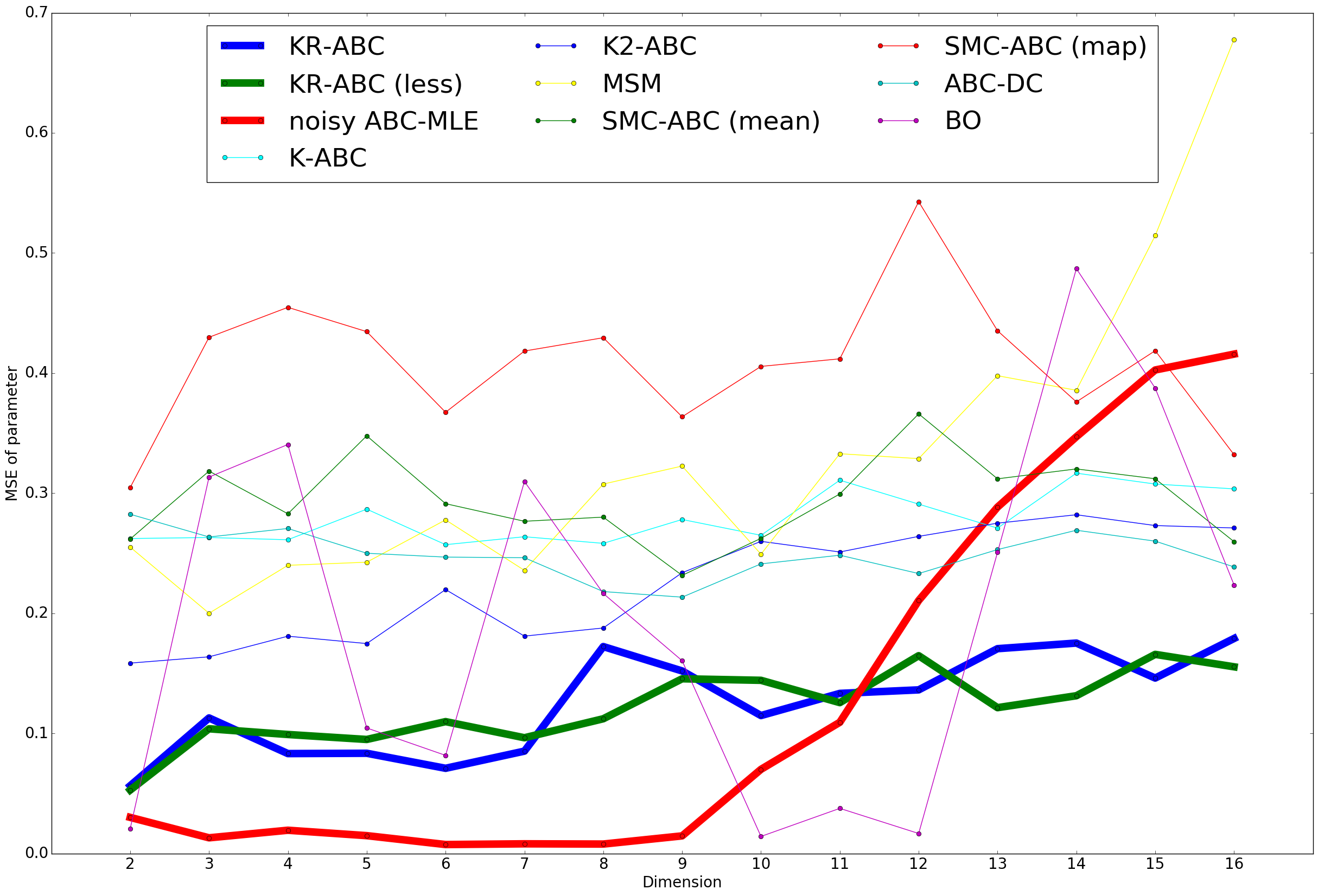
Figure 1: Results for multivariate elliptically contoured alpha stable distributions in Sec. 4.4. For each dimension (vertical axis), the averages of mean squared errors (MSE) over 30 trials are shown.

4.5 Gaussian mixture with redundant components

We consider here a parametric model in which there exist redundant parameters for expressing given data. We are interested in whether point estimation with the proposed method results in elimination of the redundant parameters when applied to such a model. This was motivated by Yamazaki and Kaji (2013), who argued that, for mixture models, the use of a Dirichlet prior with a sufficiently small concentration parameter leads to elimination of unnecessary components. We therefore focus on mixture models with redundant components.

Specifically, we considered Gaussian mixture models. We defined the true model as a two-component Gaussian mixture $\sum_{i=1}^{2}\phi_{i}\rm{Normal}(\mu_{i},20)$ of equal variances. The task was to estimate the mixture coefficients $(\phi_{1},\phi_{2},):=(0.7,0.3)$ and the associate means $(\mu_{1},\mu_{2}):=(110,70)$, provided 3000 i.i.d. sample points from the model as observed data $y^{*}$. We employed an over-parametrized model for point estimation (i.e., no method used the knowledge that the truth consisted of 2 components), which is a four-component Gaussian mixture $\sum_{i=1}^{4}\phi_{i}\rm{Normal}(\mu_{i},20)$. We used a 4-dimensional Dirichlet distribution with equal concentration parameters $0.01$ as a prior for the coefficients $(\phi_{1},\dots,\phi_{4})$, and ${\rm Normal}(0,100)$ as a prior for each of $\mu_{1},\dots,\mu_{4}$.

For each method, we generated a total of 1000 pairs of a parameter and pseudo-data, and for iterative methods, we made use of 100 pairs in each iteration, resulting in 10 iterations. Each pseudo-data consisted of 3000 simulated observations. For all the methods, we converted each data item into a histogram of 300 bins and treated it as a 300 dim. vector since this resulted in better performances. We set the parameter $\alpha\in(0,1)$ of SMC-ABC to be 0.2, as this performed well in this experiment.

We ran each algorithm 30 times, and the resulting average errors and standard deviations are shown in Table 3, where the $\phi$ error and $\mu$ error denote the errors for the coefficients and the means, respectively, as measured in terms of Euclidean distance. More precisely, since any permutation of component labels will result in the same model, we first sorted the estimated parameters $\{(\phi_{i},\mu_{i})\}$ so that $\phi_{1}\geq\cdots\geq\phi_{4}$, and we then measured the errors w.r.t. the ground truth $\phi:=(0.7,0.3,0,0)$ and $\mu:=(110,70)$. For the $\mu$ error, we computed the errors only for the estimated means $\mu_{1},\mu_{2}$ associated with the two largest coefficients since there was no ground truth for the redundant components $\mu_{3},\mu_{4}$. Results show that the proposed KR-ABC performed best, indicating that the dominant components were successfully estimated.

Table 3: Results for the Gaussian mixture model in Sec. 4.5

Algorithm $\phi$ error $\mu$ error data error cputime KR-ABC 0.159(0.106) 54.14(8.71) 0.03(0.05) 281.59(12.55) KR-ABC (less) 0.22(0.13) 64.04(17.58) 0.11(0.15) 147.39(16.76) K2-ABC 0.53(0.02) 93.98(3.84) 0.69(0.10) 89.43(7.56) K-ABC 0.50(0.02) 92.57(12.77) 0.67(0.17) 135.01(11.35) SMC-ABC (mean) 0.51(0.04) 83.19(27.86) 0.23(0.15) 214.35(8.77) SMC-ABC (MAP) 0.21(0.13) 72.76(56.24) 0.12(0.08) 214.35(8.77) ABC-DC 0.48(0.16) 137.84(50.06) 0.43(0.14) 149.74(21.22) BO 0.37(0.08) 80.79(36.17) 0.82(0.68) 13775.48(1438.9) MSM 0.24(0.08) 117.02(11.48) 0.24(0.08) 171.58(59.38)

4.6 Real-world pedestrian simulator

Our final experiment was parameter estimation with CrowdWalk, a publicly available real-world simulator for the movements of pedestrians in a commercial district (Yamashita et al., 2010). It has been used to gain insights into pedestrian behavior at a variety of events and occurrences, such as fireworks festivals and evacuations after earthquakes. As this simulator is complicated and also computationally expensive, its likelihood function is intractable.

Using CrowdWalk, we simulated the movements of pedestrians in Ginza, a commercial district in Tokyo (see Supplementary Materials for an illustration). Specifically, we modeled pedestrians as a mixture of multiple groups, each of which has the following 6 parameters (below $i$ denotes the index of a group): (1) $\theta^{(N)}_{i}\in\mathbb{N}$: the number of pedestrians in the group; (2) $\theta^{(T)}_{i}\in\mathbb{R}_{+}$: the time when the group starts to move; (3) $\theta^{(S)}_{i}\in\mathbb{R}^{2}$: the starting location of the group (e.g., stations); (4) $\theta^{(G)}_{i}\in\mathbb{R}^{2}$: the goal location of the group; (5) $\theta^{(P)}_{i}\in\mathbb{R}^{2}$: the intermediate location(s) that the pedestrians in the group visit (e.g., stores); and (6) $\theta^{(R)}_{i}\in\mathbb{R}_{+}$: the time duration(s) of the pedestrians’ visit(s) at the intermediate location(s).

In this experiment, we focused on estimation of the first two parameters $\theta^{(N)}_{i}$, $\theta^{(T)}_{i}$, and fixed the other parameters. We defined the true model as a mixture of 5 pedestrian groups, and set their parameters as $(\theta^{*(N)}_{1},\dots,\theta^{*(N)}_{5}):=(100,100,100,100,100)$ and $(\theta^{*(T)}_{1},\dots,\theta^{*(T)}_{5}):=(30,60,90,120,150)$. As in Sec. 4.5, we used a redundant model of a mixture of 10 groups for parameter estimation. The goal was to detect the active 5 groups of the true model, without knowing that the truth consists of 5 groups. For simplicity, 5 (unknown) groups among the 10 candidate groups included the parameters of the true model other than $\theta^{*(N)}_{i}$, $\theta^{*(T)}_{i}$; see the Supplementary Materials for details.

We defined prior distributions as follows. First we assumed the total number $500$ of pedestrians to be known. The mixing coefficients of the mixture of 10 groups are given by $(\phi_{1},\dots,\phi_{10})=(\theta^{(N)}_{1},\dots,\theta^{(N)}_{10})/500$. Thus, rather than directly putting a prior on $(\theta^{(N)}_{1},\dots,\theta^{(N)}_{10})$, we defined a prior on the mixing coefficients $(\phi_{1},\dots,\phi_{10})$. Specifically, we used a Dirichlet prior with a small concentration parameter, as in Sec. 4.5, in order to eliminate 5 redundant components:

$$(\phi_{1},\dots,\phi_{10}) \sim {\rm Dirichlet}(\alpha_{1},...,\alpha_{10}),$$

$$\theta^{(N)}_{i} := \phi_{i}*500,\quad(i=1,\dots,10)$$

where $\alpha_{1}=\cdots=\alpha_{10}=0.01$ denote the concentration parameters. For each of $\theta^{(T)}_{1},\dots,\theta^{(T)}_{10}$, we defined a broad uniform prior $\theta^{(T)}_{i}\sim{\rm Unif}(0,480)$.

From the true model, we simulated 4200 time steps of pedestrian flow as observed data. We made $5\times 5=25$ grids in a map of Ginza and computed a histogram of the corresponding 25 bins for each time step. Thus, observed data was made up of 4200 vectors in $\mathbb{R}^{25}$. In the same way, each method generated a total of 4200 vectors, and each iterative method made use of 200 vectors in each iteration, running 21 iterations in total. For SMC-ABC, we set the parameter $\alpha\in(0,1)$ to be 0.2, as in the previous experiment.

We ran each method 20 times, and the resulting averages and standard deviations for errors are summarized in Table 4, where “$\theta^{(N)}$ error” and “$\theta^{(T)}$ error” denote the errors of the corresponding estimated parameters, as measured in terms of Euclidean distance. These errors were computed in the same way as in Sec. 4.5 (e.g., the estimated parameters were sorted according to the magnitudes of the mixing coefficients). Results show that our method performed the best, confirming its effectiveness. In the Supplementary Materials, we also report the point estimates made using the proposed method, showing that the true parameters were estimated reasonably accurately.

Table 4: Results for the pedestrian simulator in Sec. 4.6

Algorithm $\theta^{(N)}$ error $\theta^{(T)}$ error data error cputime KR-ABC 61.58(74.42) 70.93(102.08) 0.008(0.009) 2233.45(97.54) KR-ABC (less) 82.46(75.05) 134.00(161.85) 0.014(0.014) 1875.32(147.16) K2-ABC 298.94(120.71) 308.95(109.43) 0.10(0.10) 1547.32(56.31) K-ABC 354.72(145.76) 389.52(140.91) 0.12(0.09) 1773.74(84.91) SMC-ABC (mean) 271.51(104.64) 363.12(91.28) 0.09(0.07) 2017.89(110.02) SMC-ABC (MAP) 255.15(139.33) 348.43(104.74) 0.09(0.1) 2017.89(110.02) ABC-DC 273.93(136.14) 327.48(98.12) 0.09(0.14) 1984.43(59.12) BO 194.57(65.83) 291.73(105.33) 0.04(0.06) 37541.23(3047.46) MSM 453.58(89.43) 510.04(55.10) 0.24(0.17) 1869.83(49.51)

5 Summary and future work

We have proposed kernel recursive ABC for point estimation with intractable likelihood and have empirically investigated the effectiveness of this approach. While we have also provided theoretical analysis to a certain extent, there remain important theoretical topics, as discussed in Sec. 3.1, that we wish to reserve for future research.

Acknowledgements

We thank the anonymous reviewers as well as Itaru Nishioka, Itsuki Noda, Takashi Washio, Shinji Ito, Wittawat Jitkrittum, and Marie Oshima for their helpful comments and support. We also thank Shuhei Mano for providing his code. MK has been supported by the European Research Council (StG Project PANAMA). KF has been supported by JSPS KAKENHI 26280009.

Supplementary Materials

Appendix A Proofs for theoretical results

We here provide proofs for the theoretical results in Section 3 of the main text. For ease of understanding, we repeat the assumptions and the statements w.r.t. those results. The notation follows that of the main text.

Assumption 1.

(i) $\ell$ has a unique global maximum at $\theta_{\infty}\in\Theta$, and $\pi(\theta_{\infty})>0$; (ii) $\pi$ is continuous at $\theta_{\infty}$, $\ell$ has continuous second derivatives in the neighborhood of $\theta_{\infty}$, and the Hessian of $\ell$ at $\theta_{\infty}$ is strictly negative-definite.

Proposition 1.

Let $\Theta\subset\mathbb{R}^{d}$ be a Borel measurable set, $k:\Theta\times\Theta\to\mathbb{R}$ be a continuous, bounded kernel, and ${\mathcal{H}}$ be its RKHS. If Assumption 1 holds, then we have

$$\lim_{N\to\infty}\left\|\mu_{P_{N}}-k(\cdot,\theta_{\infty})\right\|_{\mathcal{H}}=0.$$

Proof.

Because Assumption 1 is equivalent to Assumptions A1, A2 and A3 in Lele et al. (2010), we can use the Corollary to Lemma A.2 on p.1624 of Lele et al. (2010); this guarantees the weak convergence of $P_{N}$ to $\delta_{\theta_{\infty}}$, the Dirac distribution at $\theta_{\infty}$. Therefore,

$$\lim_{N\to\infty}\left\|\mu_{P_{N}}-k(\cdot,\theta_{\infty})\right\|_{\mathcal{H}}^{2} = \lim_{N\to\infty}\left<\mu_{P_{N}},\mu_{P_{N}}\right>_{\mathcal{H}}-2\lim_{N\to\infty}\left<\mu_{P_{N}},k(\cdot,\theta_{\infty})\right>_{\mathcal{H}}$$

$$+\left<k(\cdot,\theta_{\infty}),k(\cdot,\theta_{\infty})\right>_{\mathcal{H}}$$

$$= \lim_{N\to\infty}\int\int k(\theta,\theta^{\prime})dP_{N}(\theta)dP_{N}(\theta^{\prime})$$

$$-2\lim_{N\to\infty}\int k(\theta,\theta_{\infty})dP_{N}(\theta)+k(\theta_{\infty},\theta_{\infty})$$

$$= k(\theta_{\infty},\theta_{\infty})-2k(\theta_{\infty},\theta_{\infty})+k(\theta_{\infty},\theta_{\infty})$$

$$= 0,$$

where (A) follows from the weak convergence of $P_{N}$ to $\delta_{\theta_{\infty}}$ and $k$ is continuous and bounded. Here we have used Theorem 2.8 (ii) in (Billingsley, 1999) for the first term in (A). ∎

Assumption 2.

(i) There exists a constant $C>0$ such that $k(\theta,\theta)=C$ for all $\theta\in\Theta$. (ii) It holds that $k(\theta,\theta^{\prime})<C$ for all $\theta,\theta^{\prime}\in\Theta$ with $\theta\neq\theta^{\prime}$.

Proposition 2.

Let $\Theta\subset\mathbb{R}^{d}$ be a compact set and $k:\Theta\times\Theta\to\mathbb{R}$ be a continuous, bounded kernel. Let $\theta_{N}:=\operatornamewithlimits{argmin}_{\tilde{\theta}\in\Theta}\left\lVert\mu_{P_{N}}-k(\cdot,\tilde{\theta})\right\rVert_{\mathcal{H}}$. If Assumptions 1 and 2 hold, then we have $\theta_{N}\to\theta_{\infty}$ as $N\to\infty$.

Proof.

By the reproducing property and Assumption 2, we have

$$\|\mu_{P_{N}}-k(\cdot,\tilde{\theta})\|_{{\mathcal{H}}}^{2} = \left\|\mu_{P_{N}}\right\|_{\mathcal{H}}^{2}-2\mu_{P_{N}}(\tilde{\theta})+k(\tilde{\theta},\tilde{\theta})$$

$$= \left\|\mu_{P_{N}}\right\|_{\mathcal{H}}^{2}-2\int k(\tilde{\theta},\theta)dP_{N}(\theta)+C.$$

Since $\int k(\tilde{\theta},\theta)dP_{N}(\theta)$ is a continuous function of $\tilde{\theta}$ (which follows from the continuity of $k$ and the dominated convergence theorem), it follows that $\|\mu_{P_{N}}-k(\cdot,\tilde{\theta})\|_{{\mathcal{H}}}^{2}$ is a continuous function of $\tilde{\theta}$, and so is $\|\mu_{P_{N}}-k(\cdot,\tilde{\theta})\|_{{\mathcal{H}}}$. Thus, since $\Theta$ is compact, $\theta_{N}=\operatornamewithlimits{argmin}_{\tilde{\theta}\in\Theta}\left\lVert\mu_{P_{N}}-k(\cdot,\tilde{\theta})\right\rVert_{\mathcal{H}}$ exists. Using the above identity, we then have

$$\theta_{N} = \operatornamewithlimits{argmin}_{\tilde{\theta}\in\Theta}\left\lVert\mu_{P_{N}}-k(\cdot,\tilde{\theta})\right\rVert_{\mathcal{H}}^{2}$$

$$= \operatornamewithlimits{argmin}_{\tilde{\theta}\in\Theta}\left\|\mu_{P_{N}}\right\|_{\mathcal{H}}^{2}-2\mu_{P_{N}}(\tilde{\theta})+C$$

$$= \operatornamewithlimits{argmax}_{\tilde{\theta}\in\Theta}\mu_{P_{N}}(\tilde{\theta}).$$

By the reproducing property, the Cauchy-Schwartz inequality, and Assumption 2, we have for all $\theta\in\Theta$

$$\left|\mu_{P_{N}}(\theta)-k(\theta,\theta_{\infty})\right| = \left|\left<k(\cdot,\theta),\mu_{P_{N}}-k(\cdot,\theta_{\infty})\right>\right|$$ (10)

$$\leq \sqrt{k(\theta,\theta)}\left\|\mu_{P_{N}}-k(\cdot,\theta_{\infty})\right\|_{\mathcal{H}}$$

$$= \sqrt{C}\left\|\mu_{P_{N}}-k(\cdot,\theta_{\infty})\right\|_{\mathcal{H}}$$

Let $\varepsilon$ be an arbitrary positive number and $U_{\varepsilon}(\theta_{\infty})$ be an open $\varepsilon$-neighborhood of $\theta_{\infty}$. From Assumption 2 (ii) and the continuity of $k$, there is $\delta>0$ such that

$$\max_{\theta\in\Theta\backslash U_{\varepsilon}(\theta_{\infty})}k(\theta,\theta_{\infty})\leq C-\delta.$$ (11)

It follows from Eq.(10) and Proposition 1 that there is $N_{0}\in\mathbb{N}$ such that

$$\max_{\theta\in\Theta}\left|\mu_{P_{N}}(\theta)-k(\theta,\theta_{\infty})\right|\leq\delta/3$$ (12)

holds for all $N\geq N_{0}$. This implies, in particular, that for all $N\geq N_{0}$

$$\mu_{P_{N}}(\theta_{\infty})\geq k(\theta_{\infty},\theta_{\infty})-\delta/3=C-\delta/3.$$ (13)

On the other hand, using Eqs.(11) and (12), we have

$$\max_{\theta\in\Theta\backslash U_{\varepsilon}(\theta_{\infty})}\mu_{P_{N}}(\theta)\leq C-\frac{2}{3}\delta$$ (14)

for all $N\geq N_{0}$.

Eqs.(13) and (14) show that the maximum of $\mu_{P_{N}}$ is attained in $U_{\varepsilon}(\theta_{\infty})$, that is, $\theta_{N}\in U_{\varepsilon}(\theta_{\infty})$, for all $N\geq N_{0}$, which completes the proof. ∎

Remark 1.

For simplicity, we assume in Proposition 2 that $\theta$ is compact, but this condition can be relaxed. For example, we may instead assume the following weaker condition: For any open neighborhood $U$ of $\theta_{\infty}$, there is a positive constant $\delta$ such that $\sup_{\theta\in\Theta\backslash U}k(\theta,\theta_{\infty})\leq k(\theta_{\infty},\theta_{\infty})-\delta$.

Appendix B Demonstration of the auto-correction mechanism for a misspecified prior

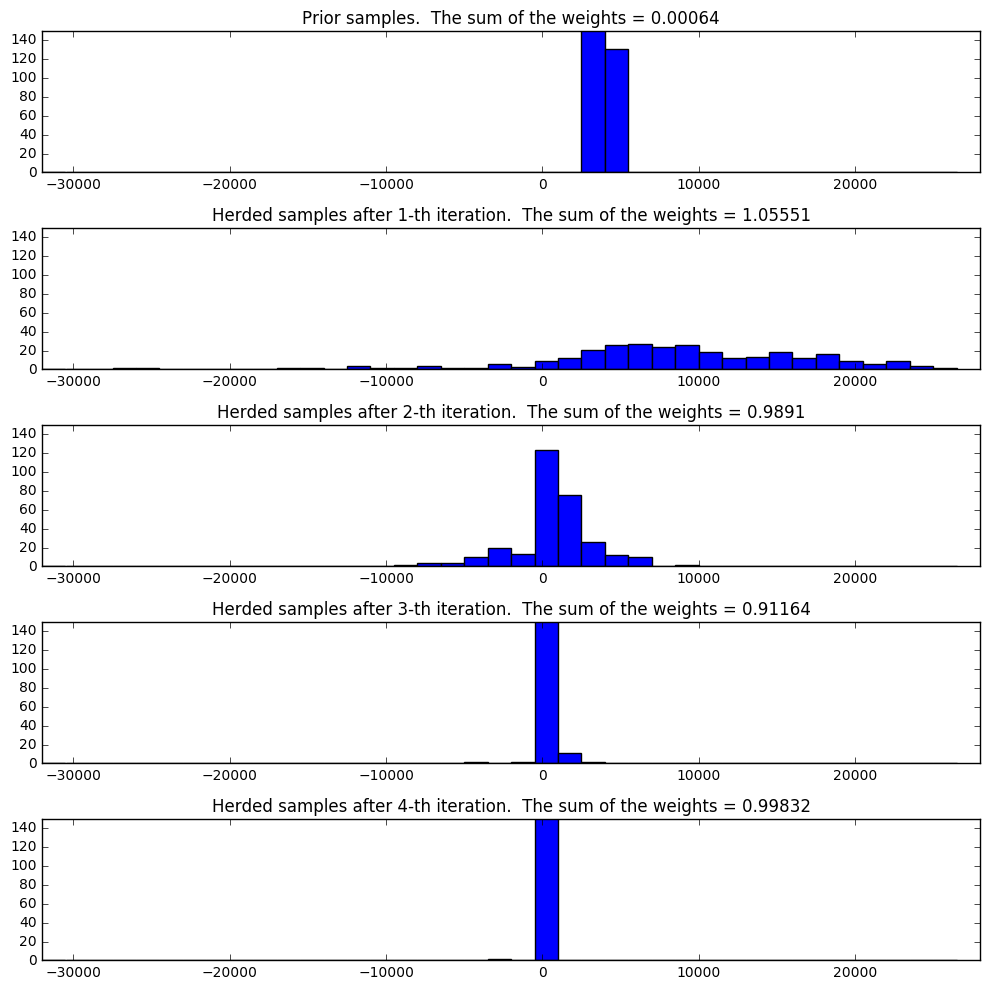
Figure 2: Each figure shows a histogram of simulated parameters for the mean of the Gaussian distribution in each iteration, as produced with the proposed method. “The sum of the weights” on the top of each figure is the sum of the weights given by kernel ABC at each iteration, as defined by Eq. (3) of the main text.

We demonstrate here how the auto-correction mechanism of the proposed method works; for an explanation of this mechanism, see Section 3 of the main text. We performed an experiment similar to the one in Section 4.2 of the main text, but under a simpler setting. The task was to estimate the mean $0$ of a univariate Gaussian distribution, ${\rm Normal}(0,40)$, provided 100 i.i.d. observations from it. The variance $40$ was assumed to be known. For the prior distribution over the mean, we used the uniform distribution on $[2000,3000]$, which is severely misspecified. For the proposed method, we recomputed the bandwidth of a Gaussian kernel for each iteration, by using the median heuristic with simulated data. In each iteration, 300 pseudo-observations were generated for the proposed method.

Figure 2 shows the results for the first 4 iterations. The top figure is a histogram of the parameters generated from the prior distribution, which, because of the misspecification of the prior, do not cover the true mean $0$. The resulting sum of the weights is $0.00064$, implying that the simulated pseudo-observations are far apart from the observed data. (As explained in the caption of Figure 2, “The sum of the weights” on the top of each figure is the sum of the weights $w_{1},\dots,w_{n}$ given by kernel ABC at each iteration, as defined by Eq. (3) of the main text.) The second figure is a histogram of the parameters generated by kernel herding in the first iteration. These parameters were generated so as to explore the parameter space, in response to the auto-correction mechanism explained in Section 3 of the main text. Since the simulated parameters were now scattered around the true mean 0, kernel ABC began to perform well from the next iteration. After only 4 iterations, the simulated parameters concentrated around the true mean.

Appendix C Supplementary to the population dynamics experiment in Section 4.3

We offer here supplementary materials for the experiment on the blowfly population dynamics in Section 4.3 of the main text.

C.1 Errors for individual parameters

Table 5: Results for blowfly population dynamics in Sec. 4.3

Algorithm $P$ $N_{0}$ $\sigma_{d}$ $\sigma_{p}$ $\tau$ $\delta$ data cputime KR-ABC 0.28(0.13) 0.03(0.05) 0.93(0.55) 1.22(0.64) 0.17(0.14) 0.17(0.15) 43.85(37.24) 101.143(13.25) KR-ABC (less) 0.15(0.13) 0.10(0.07) 1.11(0.12) 1.45(0.26) 0.23(0.41) 0.27(0.45) 67.57(47.11) 32.98(1.21) K2-ABC 1.27(1.75) 0.20(0.23) 0.98(0.42) 1.46(1.10) 0.31(0.19) 0.61(0.82) 67.45(77.86) 23.47(1.59) K-ABC 0.48(0.13) 0.14(0.06) 1.28(0.87) 1.42 (0.40) 0.22 (0.02) 0.27(0.25) 89.37(29.22) 30.66(2.57) SMC-ABC (mean) 0.58 (0.15) 0.11(0.06) 1.03(0.46) 1.98(0.32) 0.28(0.15) 1.01(0.11) 170.41 (47.91) 38.50(2.34) SMC-ABC (MAP) 0.51(0.28) 0.19(0.10) 0.89(0.33) 1.89(0.33) 0.53(0.46) 1.01(0.10) 163.19(42.51) 38.50(2.34) ABC-DC 0.48(0.22) 0.25(0.13) 1.36(0.88) 1.55(0.12) 0.54(0.31) 1.17(0.11) 134.12(58.92) 29.94(4.57) BO 0.83 (0.84) 0.16(0.24) 1.44(0.76) 1.09(0.50) 0.22(1.05) 0.45(0.41) 108.18(67.08) 3217.40(157.31) MSM 0.65(0.16) 0.26(0.19) 1.50(0.59) 1.01(0.57) 0.14(0.13) 0.51(0.15) 89.17(33.20) 25.46(8.26)

Table 5 shows the separate errors made by each method for individual parameters. This was omitted from the main text due to space constraints.

C.2 Prior distribution for the parameters of the blowfly population dynamics

We describe here the prior distribution for the parameters $\theta:=(P\in\mathbb{N},\ N_{0}\in\mathbb{N},\ \sigma_{d}\in\mathbb{R}_{+},\ \sigma_{p}\in\mathbb{R}_{+},\ \tau\in\mathbb{N},\ \delta\ \in\mathbb{R}_{+})$ in the blowfly population dynamics, the parameters that we used in our experiment. Let $\epsilon_{p},\epsilon_{N_{0}},\epsilon_{\sigma_{d}},\epsilon_{\sigma_{p}},\epsilon_{\tau},\epsilon_{\delta}\sim\rm{Normal}(0,1)$ be independent standard Gaussian random variables. The prior can then be specified by defining the parameters as such random variables as

$$P = \exp(2+2\epsilon_{p}),$$

$$N_{0} = \exp(5+0.5\epsilon_{N_{0}}),$$

$$\sigma_{d} = \exp(-0.5+\epsilon_{\sigma_{d}}),$$

$$\sigma_{p} = \exp(-0.5+\epsilon_{\sigma_{p}}),$$

$$\tau = \exp(2+\epsilon_{\tau}),$$

$$\delta = \exp(-1+0.4\epsilon_{\delta}).$$

Note that the parameters $P,N_{0},\tau$ are to be rounded appropriately, as they are defined as being natural numbers.

Appendix D Supplementary materials for the experiments on alpha stable distributions in Section 4.4

D.1 Computation time

We offer here supplementary materials for the experiment on multivariate alpha stable distributions in Section 4.4 of the main text.

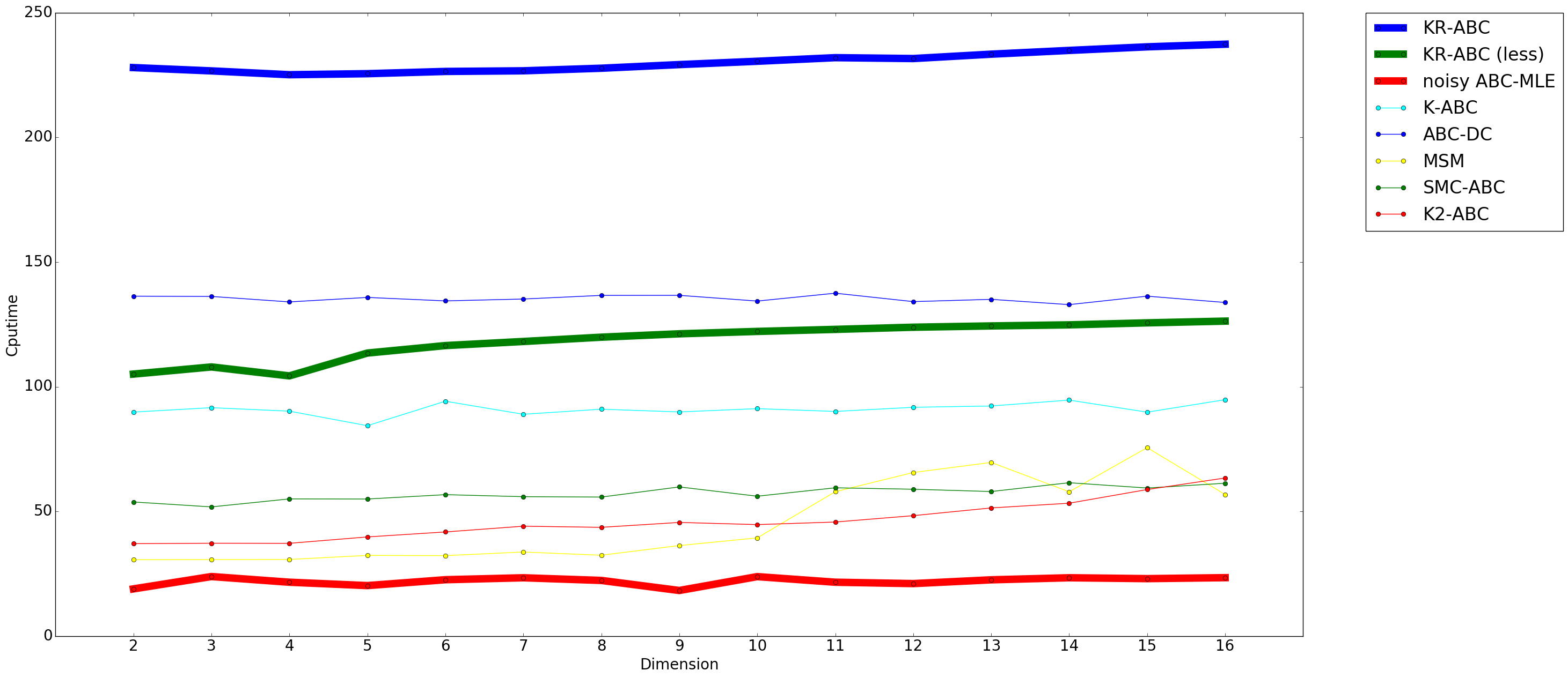
Figure 3: Computation time (in seconds) for the experiments in Section 4.4. We omit here the computation time of Bayesian optimization, but it was more than 1500 seconds for all the dimensions.

Figure 3 shows computation time for each method in the experiments on multivariate alpha stable distributions in Section 4 of the main text, which information was omitted from the main body because of space constraints.

D.2 Definition of the deterministic map for sampling

We describe here the deterministic map $\tau_{\theta}$ used in sampling multivariate alpha stable distributions (Chambers et al., 1976), where $\theta:=(\alpha,\beta,\mu,\sigma)\in(0,2]\times[-1,1]\times\mathbb{R}\times[0,\infty)$. Given $U_{1}\sim{\rm Unif}(-\pi/2,\pi/2)$ and $U_{2}\sim{\rm Exp}(1)$, the mapping $\tau_{\theta}(U_{1},U_{2})\in\mathbb{R}$ is defined as

$$\tau_{\theta}(U_{1},U_{2}):=\sigma\tau_{\alpha,\beta}(U_{1},U_{2})+\mu,$$

where

$\tau_{\alpha,\beta}(U_{1},U_{2}):=\left\{\begin{tabular}[]{@{}l@{}}$S_{\alpha,\beta}\frac{\sin[\alpha(\it{U_{1}}+B_{\alpha,\beta})]}{[\cos(\it{U_{1}})]^{1/\alpha}}(\frac{\cos[\it{U_{1}}-\alpha(U_{1}+B_{\alpha,\beta})]}{U_{2}})^{(1-\alpha)/\alpha},~{}~{}\alpha\neq 1$\\ $X=\frac{2}{\pi}[(\frac{\pi}{2}+\beta\it{U_{1}})\tan\it{U_{1}}-\beta\rm{log}(\frac{\it{U_{2}}\cos\it{U_{1}}}{\frac{\pi}{2}+\beta\it{U_{1}}})],~{}~{}\alpha=1.$\end{tabular}\right\}$

$$B_{\alpha,\beta}:=\frac{\tan^{-1}(\beta\tan\frac{\pi\alpha}{2})}{\alpha},~{}~{}~{}~{}~{}S_{\alpha,\beta}:=\left(1+\beta^{2}\tan^{2}\frac{\pi\alpha}{2}\right)^{1/2\alpha}.$$

Appendix E Supplementary material for the pedestrian simulator experiment in Section 4.6

We present here supplementary material w.r.t. the pedestrian simulator experiment in Section 4.6.

E.1 Example of simulation results obtained with CrowdWalk

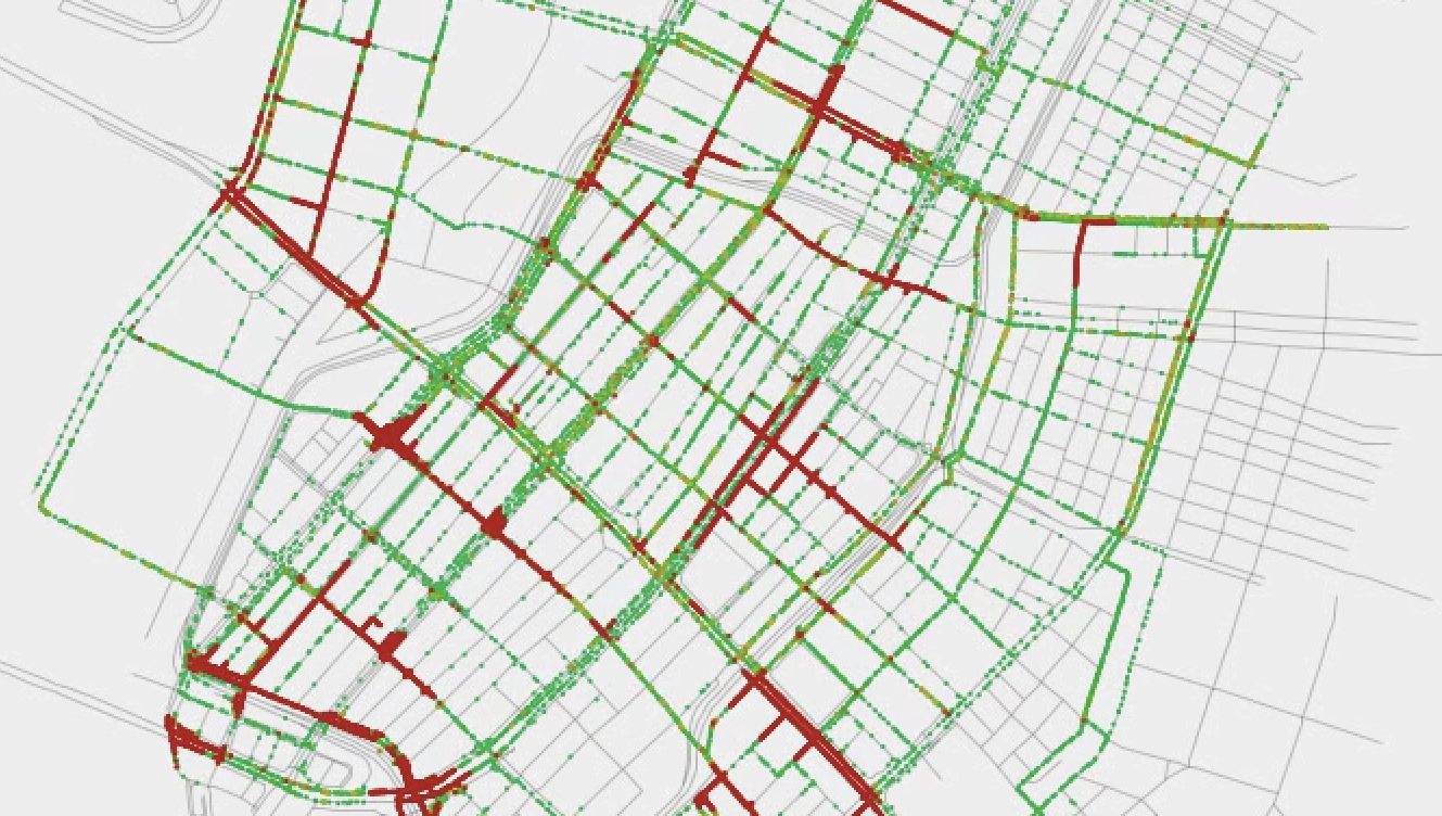
Figure 4: Example of simulation results obtained with Crowdwalk

Figure 4 shows an example of simulation results with the pedestrian flow simulator CrowdWalk (Yamashita et al., 2010). The map is of Ginza, one of the largest commercial districts in Tokyo. Both green and red points indicate pedestrians, each of which is moving at an individual speed. Red points are pedestrians who are walking particularly slowly; these pedestrians are forced to walk slowly because the areas in which they are walking are crowded.

E.2 Parameters for the pedestrian simulator

Table 6: Parameters for the pedestrian simulator, including the fixed ones

Group	$\theta^{(S)}$	$\theta^{(G)}$	$\theta^{(P)}$	$\theta^{(R)}$	$\theta^{(N)}$	$\theta^{(T)}$
1	1	0	15, 29	5400, 1800	100	30
2	5	2	24, 43	5400, 5400	100	60
3	8	3	28, 48	5400, 5400	100	90
4	4	7	2, 0	1800, 3600	100	120
5	3	2	8, 9	5400, 5400	100	150
6	6	9	26, 14	5400, 3600	0	180
7	10	11	4, 41	1800, 3600	0	210
8	2	9	50, 18	1800, 3600	0	240
9	0	6	40, 33	3600, 5400	0	270
10	11	5	20, 25	1800, 3600	0	300

Table 6 shows the parameters of the 10 candidate groups in a mixture model used for parameter estimation. Note that the parameters $\theta^{(N)}$ and $\theta^{(T)}$ were unknown for each method since they were the parameters to be estimated. Groups 1 to 5 are the components of the true model, but this fact was also unknown for each method. The numbers in $\theta^{(S)}$, $\theta^{(G)}$ and $\theta^{(P)}$ indicate certain locations on the map (e.g., the Mitsukoshi Department Store, the Apple Store, and Ginza Station), which are predefined in terms of two-dimensional coordinates. The parameter $\theta^{(P)}$ indicates certain places where pedestrians in a single group visit. In this experiment, pedestrians in each group visited 2 intermediate places during the travel from the starting location to the goal; $\theta^{(R)}$ represent the respective durations of time (in seconds) at the intermediate places. (Note that the units for starting time $\theta^{(T)}$ are in minutes.)

E.3 Estimated parameters with the proposed method

Tables 7 and 8 show the estimated values for the parameters $\theta_{i}^{(N)}$ and $\theta_{i}^{(T)}$, respectively, for each of independent 20 trials. Recall that $i$ in $\theta_{i}^{(N)}$ and $\theta_{i}^{(T)}$ is the index of 10 groups, i.e,, $i=1,\dots,10$. Results show that the proposed method was able to estimate the parameters of the 5 true groups in most cases. Note that the estimated values of $\theta_{i}^{(T)}$ for $i=6,\dots,10$ were rather arbitrary. This is reasonable since the corresponding numbers of pedestrians $\theta_{i}^{(N)}$ in these groups were estimated to be zero or very small, and thus these groups could be treated as being nonexistent.

Table 7: Estimated values of $\theta_{i}^{(N)}$ with KR-ABC for each of 20 trials

Trial	$\theta_{1}^{(N)}$	$\theta_{2}^{(N)}$	$\theta_{3}^{(N)}$	$\theta_{4}^{(N)}$	$\theta_{5}^{(N)}$	$\theta_{6}^{(N)}$	$\theta_{7}^{(N)}$	$\theta_{8}^{(N)}$	$\theta_{9}^{(N)}$	$\theta_{10}^{(N)}$
1	95	132	102	1	79	32	2	9	13	31
2	100	105	105	84	100	0	0	0	0	0
3	98	102	90	81	101	0	16	0	7	0
4	93	98	99	101	95	0	0	0	0	9
5	103	12	84	9	88	27	2	33	19	3
6	87	105	108	100	92	0	6	0	0	0
7	90	102	104	102	97	0	0	0	0	0
8	116	79	93	118	88	0	0	0	0	1
9	97	91	101	110	94	0	0	1	0	0
10	102	127	0	0	97	0	38	70	51	12
11	102	105	94	87	100	0	0	0	0	7
12	0	2	100	228	103	0	0	0	1	64
13	98	97	96	108	95	0	0	0	1	0
14	103	98	94	94	102	3	0	0	0	1
15	105	176	106	0	9	78	2	14	3	2
16	96	134	100	0	95	0	70	0	0	0
17	98	106	96	87	98	4	1	4	0	2
18	798	101	97	97	98	0	2	1	1	0
19	109	54	55	181	68	0	0	31	0	0
20	98	90	101	102	99	3	2	0	0	0

Table 8: Estimated values of $\theta_{i}^{(T)}$ with KR-ABC for each of 20 trials

Trial	$\theta_{1}^{(T)}$	$\theta_{2}^{(T)}$	$\theta_{3}^{(T)}$	$\theta_{4}^{(T)}$	$\theta_{5}^{(T)}$	$\theta_{6}^{(T)}$	$\theta_{7}^{(T)}$	$\theta_{8}^{(T)}$	$\theta_{9}^{(T)}$	$\theta_{10}^{(T)}$
1	35	56	63	289	158	91	252	216	325	209
2	25	52	87	121	152	186	152	22	193	460
3	28	53	93	119	145	110	89	201	146	18
4	29	60	92	120	147	356	188	147	249	0
5	27	66	88	229	138	85	130	54	181	236
6	22	53	85	121	151	338	208	309	31	135
7	33	61	91	120	147	2	175	214	124	396
8	26	68	95	129	136	25	375	161	81	266
9	26	59	91	125	157	18	373	0	251	0
10	30	53	452	243	151	285	69	89	175	216
11	30	57	92	111	153	279	158	369	273	169
12	213	173	92	125	154	130	77	0	456	0
13	29	54	93	125	152	346	294	327	214	490
14	34	59	89	116	150	275	36	490	37	109
15	28	54	88	135	362	70	0	319	456	0
16	29	50	88	285	146	0	403	98	286	300
17	27	54	86	121	149	22	72	310	21	93
18	30	59	89	119	146	221	107	361	218	260
19	27	74	101	119	123	211	272	206	265	275
20	30	54	87	127	146	286	452	199	267	119

Appendix F Linear time estimator for the energy distance

In a way similar to that with Gretton et al. (2012, Section 6), we define here a linear-time estimator for the energy distance (Székely and Rizzo, 2013). Let $x_{1}\dots,x_{n}\sim P$ and $y_{1},\dots,y_{n}\sim Q$ be i.i.d. samples from the two distributions $P$ and $Q$, and let $n_{2}:=\lfloor n/2\rfloor$. The linear estimator can then be defined as

$$\frac{1}{n_{2}}\sum_{i=1}^{n_{2}}h((x_{2i-1},y_{2i-1}),(x_{2i},y_{2i})),$$

where

$$h((x_{2i-1},y_{2i-1}),(x_{2i},y_{2i})):=\|x_{2i-1}-y_{2i}\|+\|x_{2i}-y_{2i-1}\|-\|x_{2i-1}-x_{2i}\|-\|y_{2i-1}-y_{2i}\|.$$

It can be easily shown that this is unbiased and converges to the population energy distance between $P$ and $Q$ at a rate of $O_{p}(n^{-1/2})$, as Gretton et al. (2012, Theorem 15) showed for a linear estimator in MMD. The above linear estimator can be computed at a cost of $O(n)$, which is less than the cost of $O(n^{2})$ required for an ordinary quadratic estimator. (Note, however, that the linear estimator has higher variance than a quadratic one.)

References

- Bach et al. (2012) Bach, F., Lacoste-Julien, S., and Obozinski, G. (2012). On the equivalence between herding and conditional gradient algorithms. In Proceedings of the 29th International Conference on Machine Learning (ICML2012), pages 1359–1366.
- Beaumont et al. (2002) Beaumont, M. A., Zhang, W., and Balding, D. J. (2002). Approximate Bayesian computation in population genetics. Genetics, 162(4), 2025–2035.
- Billingsley (1999) Billingsley, P. (1999). Convergence of Probability Measures, 2nd Edition. Wiley-Interscience.
- Brochu et al. (2010) Brochu, E., Cora, V. M., and De Freitas, N. (2010). A tutorial on Bayesian optimization of expensive cost functions, with application to active user modeling and hierarchical reinforcement learning. arXiv preprint arXiv:1012.2599.
- Chambers et al. (1976) Chambers, J. M., Mallows, C. L., and Stuck, B. (1976). A method for simulating stable random variables. Journal of the american statistical association, 71(354), 340–344.
- Chen et al. (2010) Chen, Y., Welling, M., and Smola, A. (2010). Super-samples from kernel herding. In Proceedings of the Twenty-Sixth Conference on Uncertainty in Artificial Intelligence, pages 109–116. AUAI Press.
- Dean et al. (2014) Dean, T. A., Singh, S. S., Jasra, A., and Peters, G. W. (2014). Parameter estimation for hidden Markov models with intractable likelihoods. Scandinavian Journal of Statistics, 41(4), 970–987.
- Del Moral et al. (2012) Del Moral, P., Doucet, A., and Jasra, A. (2012). An adaptive sequential Monte Carlo method for approximate Bayesian computation. Statistics and Computing, 22(5), 1009–1020.
- Dick et al. (2013) Dick, J., Kuo, F. Y., and Sloan, I. H. (2013). High dimensional numerical integration - The Quasi-Monte Carlo way. Acta Numerica, 22(133-288).
- Doucet et al. (2002) Doucet, A., Godsill, S. J., and Robert, C. P. (2002). Marginal maximum a posteriori estimation using Markov chain Monte Carlo. Statistics and Computing, 12(1), 77–84.
- Fukumizu et al. (2008) Fukumizu, K., Gretton, A., Sun, X., and Schölkopf, B. (2008). Kernel measures of conditional dependence. In Advances in neural information processing systems, pages 489–496.
- Fukumizu et al. (2013) Fukumizu, K., Song, L., and Gretton, A. (2013). Kernel Bayes’ rule: Bayesian inference with positive definite kernels. The Journal of Machine Learning Research, 14(1), 3753–3783.
- Fukunaga and Hostetler (1975) Fukunaga, K. and Hostetler, L. (1975). The estimation of the gradient of a density function, with applications in pattern recognition. IEEE Transactions on information theory, 21(1), 32–40.
- Gourieroux et al. (1993) Gourieroux, C., Monfort, A., and Renault, E. (1993). Indirect inference. Journal of applied econometrics, 8(S1).
- Gretton et al. (2007) Gretton, A., Borgwardt, K. M., Rasch, M., Schölkopf, B., and Smola, A. J. (2007). A kernel method for the two-sample-problem. In Advances in neural information processing systems, pages 513–520.
- Gretton et al. (2012) Gretton, A., Borgwardt, K. M., Rasch, M. J., Schölkopf, B., and Smola, A. (2012). A kernel two-sample test. Journal of Machine Learning Research, 13(Mar), 723–773.
- Grünewälder et al. (2012) Grünewälder, S., Lever, G., Baldassarre, L., Patterson, S., Gretton, A., and Pontil, M. (2012). Conditional mean embeddings as regressors. In Proceedings of the 29th International Conference on Machine Learning (ICML2012), pages 1823–1830.
- Gutmann and Corander (2016) Gutmann, M. U. and Corander, J. (2016). Bayesian optimization for likelihood-free inference of simulator-based statistical models. Journal of Machine Learning Research, 17(125), 1–47.
- Kanagawa et al. (2016a) Kanagawa, M., Sriperumbudur, B. K., and Fukumizu, K. (2016a). Convergence guarantees for kernel-based quadrature rules in misspecified settings. In D. D. Lee, M. Sugiyama, U. V. Luxburg, I. Guyon, and R. Garnett, editors, Advances in Neural Information Processing Systems 29, pages 3288–3296. Curran Associates, Inc.
- Kanagawa et al. (2016b) Kanagawa, M., Nishiyama, Y., Gretton, A., and Fukumizu, K. (2016b). Filtering with state-observation examples via kernel Monte Carlo filter. Neural Computation, 28(2), 382–444.
- Lacoste-Julien et al. (2015) Lacoste-Julien, S., Lindsten, F., and Bach, F. (2015). Sequential kernel herding: Frank-Wolfe optimization for particle filtering. In G. Lebanon and S. V. N. Vishwanathan, editors, Proceedings of the 18th International Conference on Artificial Intelligence and Statistics, volume 38 of Proceedings of Machine Learning Research, pages 544–552. PMLR.
- Lele et al. (2010) Lele, S. R., Nadeem, K., , and Schmuland, B. (2010). Estimability and likelihood inference for generalized linear mixed models using data cloning. Journal of the American Statistical Association, 105(492), 1617–1625.
- Marjoram et al. (2003) Marjoram, P., Molitor, J., Plagnol, V., and Tavaré, S. (2003). Markov chain Monte Carlo without likelihood. Proceedings of the National Academy of Sciences, 100(26), 15324–15328.
- McFadden (1989) McFadden, D. (1989). A method of simulated moments for estimation of discrete response models without numerical integration. Econometrica: Journal of the Econometric Society, pages 995–1026.
- Meeds and Welling (2014) Meeds, E. and Welling, M. (2014). GPS-ABC: Gaussian process surrogate approximate Bayesian computation. In Proceedings of the Thirtieth Conference on Uncertainty in Artificial Intelligence, pages 593–602. AUAI Press.
- Mitrovic et al. (2016) Mitrovic, J., Sejdinovic, D., and Teh, Y.-W. (2016). DR-ABC: approximate Bayesian computation with kernel-based distribution regression. In International Conference on Machine Learning, pages 1482–1491.
- Muandet et al. (2017) Muandet, K., Fukumizu, K., Sriperumbudur, B. K., and Schölkopf, B. (2017). Kernel mean embedding of distributions : A review and beyond. Foundations and Trends in Machine Learning, 10(1–2), 1–141.
- Nakagome et al. (2013) Nakagome, S., Fukumizu, K., and Mano, S. (2013). Kernel approximate Bayesian computation in population genetic inferences. Statistical applications in genetics and molecular biology, 12(6), 667–678.
- Nolan (2013) Nolan, J. P. (2013). Multivariate elliptically contoured stable distributions: theory and estimation. Computational Statistics, 28(5), 2067–2089.
- Park et al. (2016) Park, M., Jitkrittum, W., and Sejdinovic, D. (2016). K2-ABC: Approximate Bayesian computation with kernel embeddings. In A. Gretton and C. C. Robert, editors, Proceedings of the 19th International Conference on Artificial Intelligence and Statistics, volume 51 of Proceedings of Machine Learning Research, pages 398–407, Cadiz, Spain. PMLR.
- Picchini and Anderson (2017) Picchini, U. and Anderson, R. (2017). Approximate maximum likelihood estimation using data-cloning abc. Computational Statistics & Data Analysis, 105, 166–183.
- Pritchard et al. (1999) Pritchard, J. K., Seielstad, M. T., Perez-Lezaun, A., and Feldman, M. W. (1999). Population growth of human y chromosomes: a study of y chromosome microsatellites. Molecular biology and evolution, 16(12), 1791–1798.
- Rubio et al. (2013) Rubio, F. J., Johansen, A. M., et al. (2013). A simple approach to maximum intractable likelihood estimation. Electronic Journal of Statistics, 7, 1632–1654.
- Smola et al. (2007) Smola, A., Gretton, A., Song, L., and Schölkopf, B. (2007). A Hilbert space embedding for distributions. In Proceedings of the International Conference on Algorithmic Learning Theory, volume 4754, pages 13–31. Springer.
- Snoek et al. (2012) Snoek, J., Larochelle, H., and Adams, R. P. (2012). Practical Bayesian optimization of machine learning algorithms. In Advances in neural information processing systems, pages 2951–2959.
- Song et al. (2009) Song, L., Huang, J., Smola, A., and Fukumizu, K. (2009). Hilbert space embeddings of conditional distributions with applications to dynamical systems. In Proceedings of the 26th Annual International Conference on Machine Learning, pages 961–968. ACM.
- Song et al. (2013) Song, L., Fukumizu, K., and Gretton, A. (2013). Kernel embeddings of conditional distributions: A unified kernel framework for nonparametric inference in graphical models. IEEE Signal Processing Magazine, 30(4), 98–111.
- Sriperumbudur et al. (2010) Sriperumbudur, B. K., Gretton, A., Fukumizu, K., Schölkopf, B., and Lanckriet, G. R. (2010). Hilbert space embeddings and metrics on probability measures. Jounal of Machine Learning Research, 11, 1517–1561.
- Székely and Rizzo (2013) Székely, G. J. and Rizzo, M. L. (2013). Energy statistics: A class of statistics based on distances. Journal of statistical planning and inference, 143(8), 1249–1272.
- Takeuchi et al. (2006) Takeuchi, I., Le, Q. V., Sears, T. D., and Smola, A. J. (2006). Nonparametric quantile estimation. Journal of Machine Learning Research, 7(Jul), 1231–1264.
- Tavaré et al. (1997) Tavaré, S., Balding, D. J., Griffiths, R. C., and Donnelly, P. (1997). Inferring coalescence times from DNA sequence data. Genetics, 145(2), 505–518.
- Toni et al. (2009) Toni, T., Welch, D., Strelkowa, N., Ipsen, A., and Stumpf, M. P. (2009). Approximate Bayesian computation scheme for parameter inference and model selection in dynamical systems. Journal of the Royal Society Interface, 6(31), 187–202.
- Wood (2010) Wood, S. N. (2010). Statistical inference for noisy nonlinear ecological dynamic systems. Nature, 466(7310), 1120–4.
- Yamashita et al. (2010) Yamashita, T., Soeda, S., and Noda, I. (2010). Assistance of evacuation planning with high-speed network model-based pedestrian simulator. In Proceedings of Fifth International Conference on Pedestrian and Evacuation Dynamics (PED 2010), page 58. PED 2010.
- Yamazaki and Kaji (2013) Yamazaki, K. and Kaji, D. (2013). Comparing two Bayes methods based on the free energy functions in Bernoulli mixtures. Neural Networks, 44, 36–43.
- Yıldırım et al. (2015) Yıldırım, S., Singh, S. S., Dean, T., and Jasra, A. (2015). Parameter estimation in hidden Markov models with intractable likelihoods using sequential Monte Carlo. Journal of Computational and Graphical Statistics, 24(3), 846–865.