A role of asymmetry in linear response of globally coupled oscillator systems

Abstract

The linear response is studied in globally coupled oscillator systems including the Kuramoto model. We develop a linear response theory which can be applied to systems whose coupling functions are generic. Based on the theory, we examine the role of asymmetry introduced to the natural frequency distribution, the coupling function, or the coupling constants. A remarkable difference appears in coexistence of the divergence of susceptibility at the critical point and a nonzero phase gap between the order parameter and the applied external force. The coexistence is not allowed by the asymmetry in the natural frequency distribution but can be realized by the other two types of asymmetry. This theoretical prediction and the coupling-constant dependence of the susceptibility are numerically verified by performing simulations in $N$-body systems and in reduced systems obtained with the aid of the Ott-Antonsen ansatz.

I Introduction

Coupled oscillator models describe the synchronization among rhythmic elements. A simple class of interaction is the global all-to-all couplings, which govern dynamics through the mean field. The Kuramoto model kuramoto-75 ; kuramoto-03 ; strogatz-00 is a paradigmatic mean-field model, which consists of phase oscillators having natural frequencies and interacting with each other through a fundamental-harmonic sine coupling function. This model provides the synchronization transition between the nonsynchronized state and partially synchronized states. The transition is continuous for the unimodal symmetric natural frequency distributions kuramoto-75 ; kuramoto-84 and can be discontinuous for bimodal symmetric ones martens-barreto-strogatz-ott-so-antonsen-09 ; pazo-montbrio-09 .

The studies mentioned above are based on the assumption of symmetry. There is no asymmetry neither in the natural frequency distribution nor in the odd symmetric coupling function. However, the symmetry might not be always guaranteed in nature, and the roles of asymmetry has to be studied accordingly. For instance, asymmetry can modify types of transitions, and nonstandard bifurcation diagrams were found with asymmetric natural frequency distributions basnarkov-urumov-07 ; basnarkov-urumov-08 ; terada-ito-aoyagi-yamaguchi-17 , and with the phase-lag parameter, which breaks the odd symmetry of coupling function omelchenko-wolfrum-12 ; omelchenko-wolfrum-13 . Another type of asymmetry is brought by weighted-coupling constants depending on the oscillators. This heterogeneity induces the asymmetry in the interaction, as a recipient and a sender are not equivalent. Dynamics of such systems have been studied recently zhou-chen-bi-hu-liu-guan2015 ; xu-gao-xiang-jia-guan-zheng-16 ; qiu-zhang-liu-bi-boccaletti-liu-guan-15 ; xiao-jia-xu-lu-zheng-17 .

Asymmetry has been also investigated in the linear response to external forces. In the Kuramoto model, the linear response was firstly derived by using the explicit forms of stationary states without assuming the symmetry of the natural frequency distribution sakaguchi-88 . According to the reported linear response formula, one can find two remarkable phenomena, which are the divergence of susceptibility, and the phase gap between the order parameter and the external force. We stress that, in the Kuramoto model, these two phenomena never coexist. It is impossible to observe the divergent susceptibility with keeping the nonzero phase gap even if the natural frequency distribution is asymmetric. The suppression of the susceptibility is also reported in a system with weighted-coupling constants, where the susceptibility is constant in the nonsynchronized state irrespective of strength of the couplings daido-15 .

In this paper we focus on the linear response, and study the role of asymmetry by comparing three types of asymmetry introduced in the Kuramoto model: the natural frequency distribution, the coupling function, and the coupling constants. Looking back to the previous works on the linear response, some natural questions should arise: Can we explain the above results in a unified manner? Is it possible to have the divergence of the susceptibility in systems with weighted-coupling constants? Can the divergence and the phase gap coexist by introducing asymmetry apart from the natural frequency distribution? We will answer these questions by developing the linear response theory.

For simplifying discussions, we concentrate on systems having only a fundamental-harmonic sine coupling function in the main text. In this type of systems, the linear response formula can be obtained through the self-consistent equation for the order parameter by using the explicit expression of stationary states sakaguchi-88 ; daido-15 . However, inspired by the linear response theory in globally coupled Hamiltonian systems patelli-gupta-nardini-ruffo-12 ; ogawa-yamaguchi-12 , we introduce another strategy of solving dynamics directly. This strategy has an advantage that it can be straightforwardly extended to systems having general coupling functions, while the self-consistent strategy can not, since there are several stationary states for a given coupling function komarov-pikovsky-13 ; komarov-pikovsky-14 ; li-ma-li-yang-14 . Another advantage of our strategy is that the direct analysis of the dynamics naturally combines the linear response analysis with the stability analysis, which is necessary to guarantee stability of reference states.

This article is organized as follows. In Sec. II we introduce a coupled oscillator model including the three types of asymmetry. The linear response theory for the nonsynchronized state is developed in Sec. III. Conditions for realizing the divergence of susceptibility and the phase gap are discussed in Sec. IV with an explanation of the constant susceptibility in a class of systems having weighted-coupling constants. The linear response with each type of asymmetry is reported in Sec. V with focusing on the coexistence of the divergence and the phase gap. Theoretical predictions are examined numerically in Sec. VI. The final section VII is devoted to the summary and discussions.

II Model

The phase reduction technique kuramoto-03 ; hoppensteadt-izhikevich-12 ; nakao-16 reduces a wide class of coupled limit-cycle oscillators with external forces, and their phase dynamics are expressed by the equation

$$\frac{d\theta_{j}}{dt}=\omega_{j}+\sum_{k=1}^{N}\Gamma_{jk}\left(\theta_{j}-\theta_{k}\right)+H_{j}\left(\theta_{j},t\right),$$ (1)

where $\theta_{j}$ and $\omega_{j}$ are the phase and natural frequency of the $j$th oscillator. We assume that $\omega_{j}$ follows a natural frequency distribution $g(\omega)$. The functions $\Gamma_{jk}(\theta)$ and $H_{j}(\theta,t)$, which are $2\pi$-periodic with respect to $\theta$, represent the interaction between the $j$th and $k$th oscillators, and the external force applied to the $j$th oscillator, respectively. We note that the argument of the coupling function $\Gamma_{jk}$ is the phase difference, which is derived by the averaging method kuramoto-03 ; hoppensteadt-izhikevich-12 ; nakao-16 .

In neuronal context a neuron has specific properties for its sensitivity and interaction. Different cells are known to exhibit various types of responses to external inputs dayan-abbott-01 . On the other hand, as a sender of a signal, the firing of the excitatory neuron increases the potentials of other neurons while that of inhibitory decreases them. This property is associated with positive and negative couplings with no-phase-lag sine function hong-strogatz-11 . The heterogeneity in coupling types is ubiquitous in nature and society and it is desirable to incorporate it to a mathematical model.

Thus, in the main text, we keep the above heterogeneity but restrict ourselves to the system

$$\frac{d\theta_{j}}{dt}=\omega_{j}-\frac{K}{N}\sum_{k=1}^{N}\sigma_{j}\rho_{k}\sin(\theta_{j}-\theta_{k}+\alpha)-h\sin(\theta_{j}-\omega_{\text{ex}}t),$$ (2)

where the second and the third terms in the right-hand-side represent the interaction and the external force, respectively. The real parameter $\alpha$ $(|\alpha|<\pi/2)$ is the phase-lag parameter sakaguchi-kuramoto-86 ; omelchenko-wolfrum-12 ; omelchenko-wolfrum-13 . The real non-negative $h$ expresses the strength of the external force, and the real $\omega_{\rm ex}$ is its frequency. The parameters $K$, $\sigma_{j}$ and $\rho_{k}$ are also real, and $\sigma_{j}$ and $\rho_{k}$ determine contribution to the coupling strength from the recipient $j$ and the sender $k$, respectively, as shown in Fig. 1. These parameters give the oscillators intrinsic coupling properties and bring the heterogeneity to the network. We can reproduce the output oriented model $\sigma_{j}\rho_{k}=\rho_{k}$ paissan-zanette-08 , the input oriented model $\sigma_{j}\rho_{k}=\sigma_{j}$ hong-strogatz-11 ; iatsenko-petkoski-mcclintock-stefanovska-13 , and symmetric input-output model $\sigma_{j}\rho_{k}=\sigma_{j}\sigma_{k}$ daido-87 ; daido-15 .

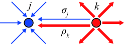
Figure 1: (Color online) Schematic picture of the coupling between the $j$th recipient and $k$th sender oscillators. The strength of coupling is $K\sigma_{j}\rho_{k}/N$.

Throughout this paper we call the model (2) the weighted-coupling model. The weighted-coupling model includes the Sakaguchi-Kuramoto model by setting $\sigma\equiv\rho\equiv 1$, where $\sigma\equiv 1$ means $\sigma_{j}=1~{}(j=1,\cdots,N)$, for instance, and the Kuramoto model by $\alpha=0$ in addition.

To measure the extent of synchrony we employ the order parameter defined by

$$z=\frac{1}{N}\sum_{j=1}^{N}e^{i\theta_{j}}.$$ (3)

Moreover, by introducing the other order parameter

$$w=\dfrac{1}{N}\sum_{j=1}^{N}\rho_{j}e^{i\theta_{j}},$$ (4)

the equation of motion (2) is rewritten as

$$\begin{split}\dfrac{d\theta_{j}}{dt}=\omega_{j}&+\frac{1}{2i}(Ke^{-i\alpha}\sigma_{j}w+he^{i\omega_{\text{ex}}t})e^{-i\theta_{j}}\\ &-\frac{1}{2i}(Ke^{i\alpha}\sigma_{j}\bar{w}+he^{-i\omega_{\text{ex}}t})e^{i\theta_{j}},\end{split}$$ (5)

where $\bar{w}$ is the complex conjugate of $w$.

The expression (5) is helpful for introducing the limit of large population, $N\to\infty$. The conservation of the number of oscillators induces the equation of continuity lancellotti-05

$$\dfrac{\partial f}{\partial t}+\dfrac{\partial}{\partial\theta}(vf)=0,$$ (6)

where $f(\theta,\omega,\sigma,\rho,t)$ is the probability density function with the normalization condition

$$\int_{0}^{2\pi}d\theta\int_{-\infty}^{\infty}d\omega\int_{-\infty}^{\infty}d\sigma\int_{-\infty}^{\infty}d\rho\,f(\theta,\omega,\sigma,\rho,t)=1.$$ (7)

The natural frequency distribution $g(\omega)$ is recovered by integrating over $\theta,\sigma$ and $\rho$ as

$$g(\omega)=\int_{0}^{2\pi}d\theta\int_{-\infty}^{\infty}d\sigma\int_{-\infty}^{\infty}d\rho\,f(\theta,\omega,\sigma,\rho,t).$$ (8)

We note that the left-hand side of (8) does not depend on the time $t$ since the natural frequency is supposed to be constant in time. The two order parameters $z$ and $w$ are defined by replacing the average over particles with the average over $f$ as

$$z(t)=\int_{0}^{2\pi}d\theta\int_{-\infty}^{\infty}d\omega\int_{-\infty}^{\infty}d\sigma\int_{-\infty}^{\infty}d\rho\,f(\theta,\omega,\sigma,\rho,t)e^{i\theta}$$ (9)

and

$$w(t)=\int_{0}^{2\pi}d\theta\int_{-\infty}^{\infty}d\omega\int_{-\infty}^{\infty}d\sigma\int_{-\infty}^{\infty}d\rho\,f(\theta,\omega,\sigma,\rho,t)\rho e^{i\theta}.$$ (10)

In terms of the order parameter $w$, the velocity field $v(\theta,\omega,\sigma,t)$ of the weighted-coupling model (2) is obtained as

$$\begin{split}v=\omega&+\dfrac{1}{2i}\left(Ke^{-i\alpha}\sigma w+he^{i\omega_{\text{ex}}t}\right)e^{-i\theta}\\ &-\dfrac{1}{2i}\left(Ke^{i\alpha}\sigma\bar{w}+he^{-i\omega_{\text{ex}}t}\right)e^{i\theta}.\end{split}$$ (11)

If the state $f(\theta,\omega,\sigma,\rho,t)$ does not depend on $\theta$, the state is called the nonsynchronized state and is denoted by $f_{0}(\omega,\sigma,\rho)$ throughout this paper. The nonsynchronized state gives $w=0$, and hence $v=\omega$ in the absence of the external force $h=0$. It is, therefore, easy to check that the nonsynchronized state $f_{0}(\omega,\sigma,\rho)$ is a stationary solution to the equation of continuity (6). In the next section III we linearize the equation of continuity (6) around the nonsynchronized state $f_{0}$, and solve it up to the leading order of a small external force $h$ to obtain the linear response.

III Linear response formula

III.1 Solution to linearized equation

We consider the stable nonsynchronized state $f_{0}(\omega,\sigma,\rho)$ for $t<0$ with the zero external force $h=0$, and a small external force is turned on at $t=0$. Due to the external force the state for $t>0$ is modified from $f_{0}$ to

$$f(\theta,\omega,\sigma,\rho,t)=f_{0}(\omega,\sigma,\rho)+f_{1}(\theta,\omega,\sigma,\rho,t).$$ (12)

Associated with the above expansion of $f$, the velocity field $v$ is also expanded as

$$v(\theta,\omega,\sigma,t)=\omega+v_{1}(\theta,\sigma,t),$$ (13)

where

$$\begin{split}v_{1}(\theta,\sigma,t)&=\dfrac{1}{2i}\left(Ke^{-i\alpha}\sigma w+he^{i\omega_{\rm ex}t}\right)e^{-i\theta}\\ &-\dfrac{1}{2i}\left(Ke^{i\alpha}\sigma\bar{w}+he^{-i\omega_{\rm ex}t}\right)e^{i\theta}\end{split}$$ (14)

and

$$w=\int_{0}^{2\pi}d\theta\int_{-\infty}^{\infty}d\omega\int_{-\infty}^{\infty}d\sigma\int_{-\infty}^{\infty}d\rho\,f_{1}(\theta,\omega,\sigma,\rho,t)\rho e^{i\theta}.$$ (15)

We note that $f_{1},v_{1}$ and $w$ come from the applied small external force, and we may assume that they are also small. The linearized equation is, therefore, obtained as

$$\dfrac{\partial f_{1}}{\partial t}+\omega\dfrac{\partial f_{1}}{\partial\theta}+f_{0}(\omega,\sigma,\rho)\dfrac{\partial v_{1}}{\partial\theta}=0.$$ (16)

As $f_{1}$ is small, the order parameter $z$,

$$z=\int_{0}^{2\pi}d\theta\int_{-\infty}^{\infty}d\omega\int_{-\infty}^{\infty}d\sigma\int_{-\infty}^{\infty}d\rho\,f_{1}(\theta,\omega,\sigma,\rho,t)e^{i\theta},$$ (17)

is also small. Our job is to calculate $z(t)$ for large $t$.

To solve the linearized equation (16), we perform the Fourier series expansion with respect to $\theta$ and the Laplace transform with respect to $t$. From the expression of $z$ (17), we can find that $z(t)$ is recovered from the Fourier $-1$ mode of $f_{1}$. Correspondingly, we focus on the external force of the Fourier $-1$ mode, which is denoted by

$$H(t)=he^{i\omega_{\rm ex}t}\Theta(t)$$ (18)

with the unit step function $\Theta(t)$. After some calculations described in Appendix A, for $f_{1}(\theta,\omega,\sigma,\rho,0)=0$, the Laplace transform of $z(t)$, denoted by $\hat{z}(s)$, is formally given by

$$\hat{z}(s)=\chi(s)\hat{H}(s),$$ (19)

where

$$\chi(s)=F(s)+Ke^{-i\alpha}\dfrac{F_{\sigma}(s)F_{\rho}(s)}{D_{K,\alpha}(s)},$$ (20)

and the functions $F_{X}(s)$ and $D_{K,\alpha}(s)$ are defined by

$$F_{X}(s)=\pi\int_{L}d\omega\int_{-\infty}^{\infty}d\sigma\int_{-\infty}^{\infty}d\rho\,\dfrac{Xf_{0}(\omega,\sigma,\rho)}{s-i\omega},$$ (21)

and

$$D_{K,\alpha}(s)=1-Ke^{-i\alpha}F_{\sigma\rho}(s).$$ (22)

The subscript $X$ is $X\in\{1,\sigma,\rho,\sigma\rho\}$ and we used the simple notation of $F(s)=F_{1}(s)$. The functions are defined in the region ${\rm Re}\,s>0$ to ensure convergence of the Laplace transform (see (60)) and the integral contour $L$ with respect to $\omega$ runs on the real axis. However, the functions are analytically continued to the whole complex $s$ plane by smoothly modifying the contour $L$ to avoid the singularity at $\omega=-is$ as shown in Appendix B.

The formula (19) is the base of the following discussions. This formula can be extended to general coupling functions and to general external forces beyond the fundamental-harmonics function as shown in Appendix A.

III.2 Linear response and susceptibility

Temporal evolution of the order parameter $z(t)$ is obtained by performing the inverse Laplace transform of $\hat{z}(s)$ as

$$z(t)=\dfrac{1}{2\pi i}\int_{\Gamma}ds\,\hat{z}(s)e^{st}.$$ (23)

The inverse Laplace transform picks up the singularities of $\hat{z}(s)$. More precisely, if $\hat{z}(s)$ has a simple pole at $s=s_{0}$, then $z(t)$ has the mode of $\exp(s_{0}t)$. Keeping this fact in mind we consider asymptotic behavior of $z(t)$.

We assumed that $f_{0}$ is stable, and hence, no singularity of $\hat{z}(s)$ appears in the domain ${\rm Re}\,s>0$. The poles in the domain ${\rm Re}\,s<0$ give exponentially decreasing modes. Therefore, if there are singularity points on the imaginary axis ${\rm Re}\,s=0$, the asymptotic behavior of $z(t)$ is dominated by them. Let us consider possible sources of imaginary singularities by recalling (19) and (20). We can say that the functions $F_{X}(s)$ has basically no singularity on the imaginary axis as the result of the analytic continuation. The roots of $D_{K,\alpha}(s)$ are possibly on the imaginary axis, but they accidentally appear for special values of $K$, as we have to determine the two parameters $K$ and the pure imaginary $s$ to satisfy the two conditions ${\rm Re}\,D_{K,\alpha}(s)=0$ and ${\rm Im}\,D_{K,\alpha}(s)=0$. Consequently, the remaining source of singularities on the imaginary axis is the Laplace transform of the external force, $\hat{H}(s)$.

The Laplace transform of the external force $H(t)=he^{i\omega_{\rm ex}t}\Theta(t)$ is written as

$$\hat{H}(s)=\dfrac{h}{s-i\omega_{\rm ex}},$$ (24)

and hence, the asymptotic behavior of $z(t)$ is expressed as

$$z(t)\xrightarrow{t\to+\infty}e^{i\omega_{\rm ex}t}\chi(i\omega_{\rm ex})h$$ (25)

in the linear regime. Moving to the rotating frame, the constant asymptotic response is obtained as

$$e^{-i\omega_{\rm ex}t}z(t)\xrightarrow{t\to+\infty}\chi(i\omega_{\rm ex})h.$$ (26)

From the above discussions, we call $\chi(s)$ the susceptibility here. We remark that the susceptibility is invariant under the exchange of the input parameter $\sigma$ and the output one $\rho$ from the formula (20).

IV Analysis of susceptibility

IV.1 Phase gap and divergence of susceptibility

The susceptibility formula (20) provides two notable phenomena: the phase gap and the divergence of the susceptibility.

The phase gap refers to the disagreement of the phases of the external force and the responded order parameter in the rotating frame with the frequency $\omega_{\rm ex}$. In (26), $h$ is positive real, hence the nonzero phase gap occurs if and only if

$${\rm Im}\,\chi(i\omega_{\rm ex})\neq 0\quad\text{or}\quad\chi(i\omega_{\rm ex})<0.$$ (27)

The divergence of the susceptibility $\chi(i\omega_{\rm ex})$ occurs, from the susceptibility formula (20), when

$$D_{K,\alpha}(i\omega_{\rm ex})=0$$ (28)

with the collateral condition

$$F_{\sigma}(i\omega_{\rm ex})F_{\rho}(i\omega_{\rm ex})\neq 0,$$ (29)

since the continued functions $F_{X}(s)$’s have no divergence. The real and imaginary parts of the condition (28) give $K$ and $\omega_{\rm ex}$, respectively. Indeed, $\omega_{\rm ex}$ is determined by the imaginary part

$${\rm Im}\left[e^{-i\alpha}F_{\sigma\rho}(i\omega_{\rm ex})\right]=0,$$ (30)

which does not depend on $K$, and then $K$ is given, with this $\omega_{\rm ex}$, from the real part

$$1-K{\rm Re}\left[e^{-i\alpha}F_{\sigma\rho}(i\omega_{\rm ex})\right]=0.$$ (31)

If ${\rm Re}[e^{-i\alpha}F_{\sigma\rho}(i\omega_{\rm ex})]\neq 0$, we can take the real parameter $K$ satisfing (31), and therefore, the divergence condition is reduced to selecting $\omega_{\rm ex}$ which satisfies (30).

In the Kuramoto model ($\alpha=0,\sigma\equiv\rho\equiv 0$) with symmetric $g(\omega)$, the zero external frequency $\omega_{\rm ex}=0$ satisfies the imaginary part (30) and the real part (31) gives

$$K=\dfrac{2}{\pi g(0)}.$$ (32)

This value agrees with the synchronization transition point as long as $g(\omega)$ is symmetric and unimodal kuramoto-03 . The distributions $g(\omega)$ used in Sec. VI are also unimodal and the pair $(\omega_{\rm ex},K)$ satisfying the condition (28) is unique. Thus, we call $K$ determined by the condition (31) as the critical point and denote it by $K_{\rm c}$ in the following discussions.

IV.2 Constant susceptibility in nonsynchronized state

Before progressing to the comparison of the three types of asymmetry, we explain and generalize the constant susceptibility reported in daido-15 . As in daido-15 , we assume that $\sigma$ and $\rho$ are independent from $\omega$. The nonsynchronized state is then written as

$$f_{0}(\omega,\sigma,\rho)=\dfrac{g(\omega)}{2\pi}P(\sigma,\rho).$$ (33)

This decomposition simplifies the function $F_{X}(s)$ as

$$F_{X}(s)=\left\langle X\right\rangle_{\sigma,\rho}F(s),$$ (34)

where

$$\left\langle X\right\rangle_{\sigma,\rho}=\int_{-\infty}^{\infty}d\sigma\int_{-\infty}^{\infty}d\rho\,XP(\sigma,\rho).$$ (35)

Therefore, the susceptibility (20) is also simplified as

$$\chi(s)=\left[1+\dfrac{\left\langle\sigma\right\rangle_{\sigma,\rho}\left\langle\rho\right\rangle_{\sigma,\rho}}{\left\langle\sigma\rho\right\rangle_{\sigma,\rho}}\dfrac{1-D_{K,\alpha}(s)}{D_{K,\alpha}(s)}\right]F(s).$$ (36)

Let us assume $\left\langle\sigma\right\rangle_{\sigma,\rho}=0$ or $\left\langle\rho\right\rangle_{\sigma,\rho}=0$. In this case the formula (36) immediately gives the constant susceptibility

$$\chi(i\omega_{\rm ex})=F(i\omega_{\rm ex})$$ (37)

in the nonsynchronized state, where we see that the right-hand side does not depend on the coupling strength. In daido-15 , $\left\langle\sigma\right\rangle_{\sigma,\rho}=0$ is assumed, and the constant susceptibility is a consequence of this assumption. We note that $\rho\equiv\sigma$ is also assumed in daido-15 , and the finite critical point $K_{\rm c}$ exists from (31), since $\left\langle\sigma\rho\right\rangle_{\sigma,\rho}=\left\langle\sigma^{2}\right\rangle_{\sigma,\rho}$ is positive unless $\sigma\equiv 0$.

We give two remarks for the independent case (33). First, the constant susceptibility is a special case, since $\chi$ may diverge if $\left\langle\sigma\right\rangle_{\sigma,\rho}\left\langle\rho\right\rangle_{\sigma,\rho}\neq 0$. Second, the imaginary part of the divergence condition (30) implies that $F(i\omega_{\rm ex})$ is real. Thus, $\chi(i\omega_{\rm ex})$ is also real and one of the nonzero phase gap condition, ${\rm Im}\chi(i\omega_{\rm ex})\neq 0$, is not satisfied.

V Linear response with asymmetry

We investigate the role of asymmetry in the linear response through the phase gap and the divergence of susceptibility. Asymmetry is introduced into the natural frequency distribution $g(\omega)$, the coupling function along with the phase-lag parameter $\alpha$, or the coupling constants $K\sigma_{j}\rho_{k}$. Each type of asymmetry is studied without external forces in the Kuramoto model ($\sigma\equiv\rho\equiv 1,\alpha=0$) kuramoto-03 ; basnarkov-urumov-08 , in the Sakaguchi-Kuramoto model ($\sigma\equiv\rho\equiv 1,\alpha\neq 0$) sakaguchi-kuramoto-86 ; omelchenko-wolfrum-12 , and in the frequency-weighted-coupling model ($\rho\equiv 1,\omega\equiv\sigma,\alpha=0$) xu-gao-xiang-jia-guan-zheng-16 ; qiu-zhang-liu-bi-boccaletti-liu-guan-15 , respectively. In the last model, the case $\rho\equiv 1$ is equivalent to the case $\sigma\equiv 1$ in the linear response due to the exchange symmetry between $\sigma$ and $\rho$ in the susceptibility $\chi(s)$ (20). The relation $\omega\equiv\sigma$ is introduced to break the independence (33), which gives rise to ${\rm Im}\,\chi(i\omega_{\rm ex})=0$, and the presented form of the correlation is not essential.

The susceptibilities in the three models are given in the subsection V.1. The coexistence of the two phonemena is discussed in the subsection V.2.

V.1 Susceptibility in the three models

The three models have the constant parameter $\rho\equiv 1$. Due to this constant parameter, the susceptibility is simplified as

$$\chi(s)=\dfrac{F(s)}{D_{K,\alpha}(s)}.$$ (38)

The function $D_{K,\alpha}(s)$ is written as

$$D_{K,\alpha}=1-Ke^{-i\alpha}F_{Y}(s),$$ (39)

where $Y=1$ in the Kuramoto model and the Sakaguchi-Kuramoto model, and $Y=\sigma$ in the frequency-weighted-coupling model.

At the pure imaginary point $s=i\omega_{\rm ex}$, the functions $F(s)$ and $F_{\sigma}(s)$ take the values

$$F(i\omega_{\rm ex})=\dfrac{\pi}{2}g(\omega_{\rm ex})+\dfrac{i}{2}{\rm PV}\int_{-\infty}^{\infty}d\omega\dfrac{g(\omega)}{\omega-\omega_{\rm ex}},$$ (40)

and

$$F_{\sigma}(i\omega_{\rm ex})=\dfrac{\pi}{2}\omega_{\rm ex}g(\omega_{\rm ex})+\dfrac{i}{2}{\rm PV}\int_{-\infty}^{\infty}d\omega\dfrac{\omega g(\omega)}{\omega-\omega_{\rm ex}}.$$ (41)

where PV represents the Cauchy principal value. The expression of $F_{\sigma}(i\omega_{\rm ex})$ is obtained from the correlation form $\sigma=\omega$ in the frequency-weighted-coupling model.

V.2 Coexistence of phase gap and divergence

Let us assume the divergence of the susceptibility (30), that is, $D_{K,\alpha}(i\omega_{\rm ex})$ is real. This condition is equivalent to

$${\rm Im}\left[e^{-i\alpha}F_{Y}(i\omega_{\rm ex})\right]=0,$$ (42)

and simplifies the former sufficient condition of (27) for the nonzero phase gap into

$${\rm Im}\,F(i\omega_{\rm ex})\neq 0.$$ (43)

We examine whether the phase gap condition (43) can hold under the divergence condition (42). In the followings, we assume that the support of $g(\omega)$ is the whole real axis.

In the Kuramoto model, we set $\alpha=0$ and $Y=1$. The divergence condition (42) becomes

$${\rm Im}\,F(i\omega_{\rm ex})=0,$$ (44)

and also from the condition (31) the critical point $K_{\rm c}$ is given by

$$K_{\rm c}=\dfrac{1}{{\rm Re}F(i\omega_{\rm ex})}=\dfrac{2}{\pi g(\omega_{\rm ex})}.$$ (45)

Obviously, the divergence condition (44) and the phase gap condition (43) are mutually exclusive. The other possibility for nonzero phase gap is that $\chi(i\omega_{\rm ex})$ is negative real. However, $F(i\omega_{\rm ex})=\pi g(\omega_{\rm ex})/2$ is positive real and $D_{K,0}(i\omega_{\rm ex})=1-KF(i\omega_{\rm ex})$ is also positive real for $K<K_{\rm c}$. Therefore, the susceptibility $\chi(i\omega_{\rm ex})$ is positive real and the two phenomena never coexist. This result is consistent with the previous work by the self-consistent analysis sakaguchi-88 .

In the Sakaguchi-Kuramoto model, we set $Y=1$ again but $\alpha\neq 0$. The divergence condition (42) is read as

$${\rm Im}\,F(i\omega_{\rm ex})\cos\alpha-{\rm Re}\,F(i\omega_{\rm ex})\sin\alpha=0,$$ (46)

which gives the critical point as

$$K_{\rm c}=\dfrac{2\cos\alpha}{\pi g(\omega_{\rm ex})}.$$ (47)

The condition (46) implies

$${\rm Im}\,F(i\omega_{\rm ex})={\rm Re}\,F(i\omega_{\rm ex})\tan\alpha=\dfrac{\pi}{2}g(\omega_{\rm ex})\tan\alpha,$$ (48)

and hence, the phase gap condition (43) holds for $\alpha\neq 0$.

Finally, in the frequency-weighted-coupling model, we set $\alpha=0$ but $Y=\sigma$. We have the divergence condition (42) of the form

$$0={\rm Im}\,F_{\sigma}(i\omega_{\rm ex})=\dfrac{1}{2}+\omega_{\rm ex}{\rm Im}\,F(i\omega_{\rm ex}).$$ (49)

This condition implies that $\omega_{\rm ex}\neq 0$ holds for the divergence, and is compatible with the phase gap condition (43) as

$${\rm Im}\,F(i\omega_{\rm ex})=-\dfrac{1}{2\omega_{\rm ex}}\neq 0.$$ (50)

We note that the critical point is given by

$$K_{\rm c}=\dfrac{2}{\pi\omega_{\rm ex}g(\omega_{\rm ex})}.$$ (51)

From the above discussions, we conclude that the disagreement of the two phases of $F(i\omega_{\rm ex})$ and $e^{-i\alpha}F_{Y}(i\omega_{\rm ex})$ is essential to realize the coexistence. The two quantities are identical in the Kuramoto model ($\alpha=0,Y=1$) even if the natural frequency distribution $g(\omega)$ is asymmetric, and therefore, the coexistence is impossible. However, the phase-lag parameter $\alpha$ or the difference between $F$ and $F_{Y}$ permits the coexistence.

VI Numerical simulations

We numerically examine theoretical predictions described in Sec. V.

VI.1 Family of natural frequency distributions

For considering both symmetric and asymmetric natural frequency distributions, we introduce a family of $g(\omega)$ as in terada-ito-aoyagi-yamaguchi-17 :

$$g(\omega)=\dfrac{c}{[(\omega-\Omega)^{2}+\gamma_{1}^{2}][(\omega+\Omega)^{2}+\gamma_{2}^{2}]},$$ (52)

where $\Omega\geq 0,\gamma_{1},\gamma_{2}>0$ and the normalization constant $c$ is given by

$$c=\dfrac{\gamma_{1}\gamma_{2}[(\gamma_{1}+\gamma_{2})^{2}+4\Omega^{2}]}{\pi(\gamma_{1}+\gamma_{2})}.$$ (53)

Using the scaling of the variables, we may set $\gamma_{2}=1$ without loss of generality. Moreover, we may concentrate on the region $\gamma_{1}\leq 1$ by considering the replacement of $\theta\to-\theta$. The distribution is symmetric if $\gamma_{1}=1$ or $\Omega=0$ and tends to be bimodal with large $\Omega$.

To capture the parameter dependence in the family (52), we compute the bifurcation diagram for a give set of parameters $(\gamma_{1},\Omega)$ in the reduced system for the Kuramoto model, which is derived by using the Ott-Antonsen ansatz ott-antonsen-08 ; ott-antonsen-09 (see Appendix C for the derivation). The parameter space $(\gamma_{1},\Omega)$ is roughly divided into five domains in the computed range as shown in Fig. 2: In the domain A the system undergoes only the continuous transition. The domain B represents the continuous and successive discontinuous transitions. The domains C and D include the oscillations before the discontinuous transition, where the continuous transition occur in C while it does not in D. In the domain E the system has only the discontinuous transition. The thick red lines are obtained by increasing $K$ whereas the thin blue lines by decreasing it. Two remarks are as follows. First, the two nonstandard bifurcation diagrams reported in terada-ito-aoyagi-yamaguchi-17 appear in the domains B and C, which are unveiled by introducing the asymmetry of $g(\omega)$. Second, the discontinuous transition can occur in the asymmetric unimodal distributions, which will be discussed in the last section.

To examine the susceptibility around the critical point, we select the continuous transition region. Moreover, we choose the unimodal distributions for simplicity: an asymmetric point $(\gamma_{1},\Omega)=(0.6,0.6)$ for the Kuramoto model, and a symmetric point $(0.25,0)$ for the Sakaguchi-Kuramoto model and the frequency-weighted-coupling model. Stability analysis is described in Appendix D and we confirm that the nonsynchronized state is unstable for $K>K_{\rm c}$, where $K_{\rm c}$ is given by (45), (47), or (51).

Numerical examinations are performed by $N$-body simulations and by the reduced system. Temporal evolution is computed by using the fourth-order Runge-Kutta algorithm with the time step $\Delta t=$0.1.

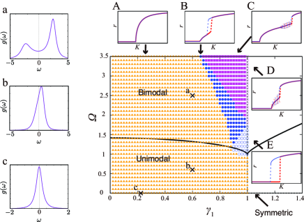
Figure 2: (Color online) Parameter space for the family (52) with $\gamma_{2}=1$. The solid black line is the border between the unimodal and bimodal regions. The distribution is symmetric on the line $\gamma_{1}=1$ or $\Omega=0$. Three representative forms of $g(\omega)$ are shown in the left panels indicated by a, b and c for the corresponding points, respectively, where the points b and c in the unimodal side are used in the numerical examinations. The five domains are A (orange filled triangle), B (blue filled circle), C(magenta filled rectangle), D (magenta open rectangle) and E (blue open circle). Each inset indicated by A, B, C, D and E shows a schematic bifurcation diagram for the Kuramoto model in the indicated domain, where the vertical bars in C and D represent the standard deviation of $r(t)$.

VI.2 The Kuramoto model

If the natural frequency distribution $g(\omega)$ is symmetric and unimodal, then the divergence condition ${\rm Im}\,F(i\omega_{\rm ex})=0$ is satisfied if and only if $\omega_{\rm ex}=0$ as shown in Appendix E. In this case the divergence of the susceptibility occurs at the critical point $K_{\rm c}=2/[\pi g(0)]$ but the phase gap is zero.

A similar thing happens for an asymmetric $g(\omega)$ with $(\gamma_{1},\Omega)=(0.6,0.6)$. The divergence remains by seeking the value $\omega_{\rm ex}\simeq 0.303819$ which satisfies the condition (44) at the critical point $K_{\rm c}\simeq 1.084618$, (45), while the phase gap vanishes. This theoretical prediction is successfully confirmed in Fig. 3, if the external force $h$ is sufficiently small, although the zero phase gap is sensitive for the strength of the external force near the critical point.

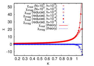
Figure 3: (Color online) Susceptibility in the Kuramoto model with an asymmetric natural frequency distribution, $(\gamma_{1},\Omega)=(0.6,0.6)$. The numerical simulations are conducted with $N=10^{5}$, $h=10^{-2}$ and $10^{-4}$. The frequency of the external force is set as $\omega_{\text{ex}}=0.303819$, which induces the zero imaginary part of the susceptibility. The divergence of $\chi(i\omega_{\rm ex})$ is observed at the critical point $K=K_{\rm c}\simeq 1.084618$, the right boundary of the panel, but no phase gap appears for sufficiently small $h$.

In contrast, when we break the divergence condition (44) by choosing $\omega_{\rm ex}=0$, the phase gap is not zero but the divergence of the susceptibility disappears. This behavior is verified in Fig.4.

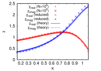
Figure 4: (Color online) Susceptibility in the Kuramoto model with an asymmetric natural frequency distribution, where $(\gamma_{1},\Omega)=(0.6,0.6)$. The numerical simulations are conducted with $N=10^{5}$ and $h=10^{-2}$. The frequency of the external force is set to zero. The phase gap appears as the nonzero imaginary part of $\chi$ but there is no divergence at the critical point $K=K_{\text{c}}\simeq 1.084618$, which is the right boundary of the panel.

VI.3 The Sakaguchi-Kuramoto model

The discussion in Sec. V.2 says that the nonzero phase gap and the divergence of the susceptibility coexists under nonzero phase-lag parameter. We use a symmetric unimodal $g(\omega)$ with $(\gamma_{1},\Omega)=(0.25,0)$. To set $\omega_{\text{ex}}=1$ satisfying the divergence condition (46), we choose the phase-lag parameter as $\alpha=-1.436475$. The critical point (47) is $K_{\rm c}\simeq 1.821283$. Under this setting, the coexistence is observed in Fig. 5 for sufficiently small $h$. We note that if $h$ is not small enough the deviation from the theoretical values is not negligible. In fact, the deviation is observed with $h=5\times 10^{-3}$ in the $N$-body and reduced systems. The deviated response suggests a kind of bifurcation with respect to the strength of external force, $h$. Studying this deviation is interesting but out of range of this article, since our main topic is the linear response.

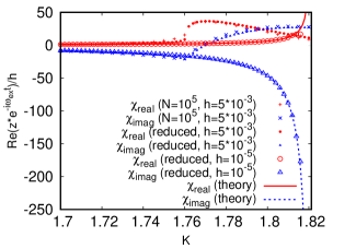
Figure 5: (Color online) Susceptibility in the Sakaguchi-Kuramoto model with $(\gamma_{1},\Omega)=(0.25,0)$. The numerical simulations are conducted with $N=10^{5}$ and $h=5\times 10^{-3},10^{-5}$. The frequency of external force is set as $\omega_{\rm ex}=1$, and the phase-lag parameter as $\alpha=-1.436475$ to satisfy the divergence condition (46). The critical point is $K_{\rm c}\simeq 1.821283$.

VI.4 The frequency-weighted-coupling model

We finally investigate the frequency-weighted-coupling model, where the coupling parameters are set as $\sigma\equiv\omega$ and $\rho\equiv 1$. The natural frequency distribution $g(\omega)$ is again taken at the point $(\gamma_{1},\Omega)=(0.25,0)$, and the phase-lag parameter is zero, $\alpha=0$. The external frequency $\omega_{\rm ex}$ is determined from the divergence condition (49) as $\omega_{\rm ex}=0.5$. The critical point (51) is calculated as $K_{\rm c}=5$.

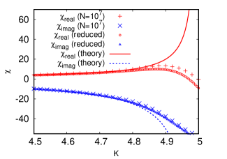
Figure 6: (Color online) Susceptibility in the frequency-weighted-coupling model with $(\gamma_{1},\Omega)=(0.25,0)$. The numerical simulations are conducted with $N=10^{7}$ and $h=10^{-3}$. The phase-lag parameter is set to zero. The frequency of the external force is given by $\omega_{\rm ex}=0.5$, which satisfies the divergence condition (49). The critical point is $K_{\rm c}=5$.

The susceptibility $\chi(i\omega_{\rm ex})$ is exhibited in Fig. 6. The theoretical curves imply the coexistence of the divergence of the susceptibility and the nonzero phase gap, but the numerically obtained values are not in good agreement with the theoretical curves near the critical point. We have two sources of this discrepancy, which are the finite-size effects and the finiteness of $h$, as observed in the Kuramoto model. We note that $h$ must be larger than the finite-size fluctuation, which may be of $O(1/\sqrt{N})$, to correctly pick up the linear response. The strength $h=10^{-3}$ is close to the boundary with $N=10^{7}$ in Fig. 6, and hence, we can not use smaller $h$.

Based on the above discussion, to verify the theoretical prediction, we computed the $N$-dependence and $h$-dependence of the absolute value of the susceptibility in Fig. 7. First, as $N$ increases with a fixed $h$, the $N$-body simulations approaches to the reduced system, which corresponds to the large population limit $N\to\infty$. Thus, the reduced system must be useful with smaller $h$. Second, the reduced system approaches to the theoretical curve as $h$ goes to $0$. We, therefore, conclude that the divergence of the susceptibility appears and it can coexist with the nonzero phase gap if the coupling parameter $\sigma$ correlates with the natural frequency $\omega$.

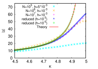
Figure 7: (Color online) $N$-dependence and $h$-dependence of the absolute values of the susceptibility in the frequency-weighted-coupling model with the parameter set $(\gamma_{1},\Omega)=(0.25,0)$.

The divergence is characterized by the critical exponent $\gamma$, defined by

$$|\chi(i\omega_{\rm ex})|\propto|K_{\rm c}-K|^{-\gamma}$$ (54)

near the critical point. The critical exponent is obtained as $\gamma=1$ in Fig. 8, which reports the convergence of the numerical points to the theoretical curve in the limit $h\to 0$. We note that the critical exponent $\gamma=1$ is also obtained by the self-consistent analysis sakaguchi-88 and by the finite-size scaling hong-chate-tang-park-15 in the Kuramoto model.

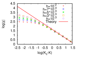
Figure 8: (Color online) Log-log plot of the absolute value of the susceptibility $|\chi(i\omega_{\rm ex})|$ against $K_{\rm c}-K$. We set the system size as $N=10^{5}$. The straight red line is obtained by the theory and has the slope $-1$.

VII Summary and discussions

We studied the role of asymmetry in coupled oscillator systems with shedding light on the linear response in the nonsynchronized state. Three types of asymmetry are considered, which appear in the natural frequency distribution, in the coupling function, or in the coupling constants. The linear response is theoretically derived by directly solving the equation of continuity up to the linear order of a small external force. To compare the three types, we focus on the coexistence of the phase gap and the divergence of the susceptibility. The asymmetry in the natural frequency distribution does not permit the coexistence, but the other two types of asymmetry do. Asymmetry in the natural frequency distribution and in the coupling function provides similar nonstandard bifurcation diagrams omelchenko-wolfrum-13 ; terada-ito-aoyagi-yamaguchi-17 . However, the two types of asymmetry are not mutually substitutable from the view point of the linear response. This result is helpful to identify an unknown system from the linear response, as the system must be beyond the description of the Kuramoto model when the coexistence is observed.

In a weighted-coupling model with the random distribution of the coupling parameters the constant susceptibility has been reported in daido-15 . Using the proposed linear response theory, we revealed that the constant susceptibility is realized under a special setting, and that the divergence of the susceptibility is possible in general.

These theoretical predictions, and the susceptibility itself, are verified by performing numerical simulations of $N$-body dynamics and of the reduced systems introduced by the Ott-Antonsen ansatz. The numerical computations suggest that we have to pay attention to the strength of the external force, since a small but rather large external force can bring a finite phase gap even if the system setting theoretically requires the zero phase gap.

The linear response theory for the first-harmonic coupling function is straightforwardly extended to general coupling functions, when we consider the nonsynchronized state. This point should be stressed as an advantage of our strategy. However, the linear response theory in the partially synchronized states has not been obtained along our line, and it must be useful for physical applications. Another interesting extension is to systems on networks beyond the all-to-all connection.

Finally, in the Kuramoto model, the asymmetry in the natural frequency distribution produces discontinuous transitions even when a distribution is unimodal. Our finding is that the discontinuity occurs with smooth distributions, while non-smooth distributions are known to cause the discontinuous transitions basnarkov-urumov-08 . We should study how the asymmetry generates the discontinuous synchronization transition with smooth unimodal distributions.

Appendix A Linear response formula in generalized system

In the main text we specifies the coupling function as only the fundamental-harmonic sine function, as in Eq. (2). However, our linear response theory is not restricted to this type of coupling function, and we here derive the expression of the susceptibility in more general systems.

We generalize the model as

$$\frac{d\theta_{j}}{dt}=\omega_{j}+\dfrac{K}{2iN}\sum_{k=1}^{N}\sigma_{j}\rho_{k}\Gamma(\theta_{j}-\theta_{k})+\frac{1}{2i}H\left(\theta_{j},t\right),$$ (55)

where $\Gamma(\theta)$ is the coupling function and $H(\theta,t)$ represents the external force. The factor $1/2i$ is multiplied for the later convenience, and is not essential. The equation of continuity is written as

$$\dfrac{\partial f}{\partial t}+\dfrac{\partial}{\partial\theta}(vf)=0,$$ (56)

where the velocity field $v\left(\theta,\omega,\sigma,t\right)$ is defined by

$$\begin{split}&v\left(\theta,\omega,\sigma,t\right)=\omega+\dfrac{1}{2i}H\left(\theta,t\right)\\ &+\dfrac{K\sigma}{2i}\int_{0}^{2\pi}d\theta^{\prime}\int_{-\infty}^{\infty}d\omega\int_{-\infty}^{\infty}d\rho\,\rho\Gamma\left(\theta-\theta^{\prime}\right)f\left(\theta^{\prime},\omega,\sigma,\rho,t\right).\end{split}$$ (57)

As in Sec.III, we expand $f$ around the nonsynchronized stationary state $f_{0}(\omega,\sigma,\rho)$ as $f=f_{0}+f_{1}$, where $f_{1}(\theta,\omega,\sigma,\rho,t)$ is regarded as a small deviation.

Let us introduce the Fourier series expansions

$$\Gamma(\theta)=\sum_{n-\infty}^{\infty}\tilde{\Gamma}(n)e^{in\theta},\quad H(\theta,t)=\sum_{n-\infty}^{\infty}\tilde{H}(n,t)e^{in\theta},$$ (58)

and

$$f_{1}(\theta,\omega,\sigma,\rho,t)=\sum_{n-\infty}^{\infty}\tilde{f}_{1}(n,\omega,\sigma,\rho,t)e^{in\theta}.$$ (59)

The Laplace transform of $Y(t)$ is defined by

$$\hat{Y}(s)=\int_{0}^{\infty}dt\,Y(t)e^{-st},\quad{\rm Re}\,s>0.$$ (60)

The condition ${\rm Re}\,s>0$ is introduced to ensure the convergence of the integral. Performing the Fourier-Laplace transform, we have the Laplace transform of $\tilde{f}_{1}$ as

$$\begin{split}&\hat{f}_{1}(-n,\omega,\sigma,\rho,s)=\dfrac{\tilde{f}_{1}(-n,\omega,\sigma,\rho,0)}{s-in\omega}\\ &+\left[K\sigma\tilde{\Gamma}(-n)\hat{w}_{n}(s)+\hat{H}(-n,s)\right]\dfrac{nf_{0}(\omega,\sigma,\rho)}{2(s-in\omega)},\end{split}$$ (61)

where $\hat{w}_{n}(s)$ is the Laplace transform of

$$\begin{split}w_{n}(t)&=\int_{0}^{2\pi}d\theta\int_{-\infty}^{\infty}d\omega\int_{-\infty}^{\infty}d\sigma\int_{-\infty}^{\infty}d\rho\,\rho e^{in\theta}f(\theta,\omega,\sigma,\rho,t)\\ &=2\pi\int_{-\infty}^{\infty}d\omega\int_{-\infty}^{\infty}d\sigma\int_{-\infty}^{\infty}d\rho\,\rho\tilde{f}_{1}(-n,\omega,\sigma,\rho,t).\end{split}$$ (62)

Another family of order parameters $z_{n}(t)$ is similarly defined by

$$\begin{split}z_{n}(t)&=\int_{0}^{2\pi}d\theta\int_{-\infty}^{\infty}d\omega\int_{-\infty}^{\infty}d\sigma\int_{-\infty}^{\infty}d\rho\,e^{in\theta}f(\theta,\omega,\sigma,\rho,t)\\ &=2\pi\int_{-\infty}^{\infty}d\omega\int_{-\infty}^{\infty}d\sigma\int_{-\infty}^{\infty}d\rho~{}\tilde{f}_{1}(-n,\omega,\sigma,\rho,t).\end{split}$$ (63)

Multipling (61) by $2\pi\rho$ and integrating over $\omega,\sigma$ and $\rho$, we have the self-consistent equation for $\hat{w}_{n}$ as

$$\hat{w}_{n}(s)= G_{\rho}(n,s)+K\tilde{\Gamma}(-n)F_{\sigma\rho}(n,s)\hat{w}_{n}(s)$$

$$+F_{\rho}(n,s)\hat{h}(-n,s).$$ (64)

The functions $F_{X}(n,s)$ and $G_{X}(n,s)$ are defined by

$$F_{X}(n,s)=\pi\int_{L}d\omega\int_{-\infty}^{\infty}d\sigma\int_{-\infty}^{\infty}d\rho\dfrac{nXf_{0}(\omega,\sigma,\rho)}{s-in\omega},$$ (65)

and

$$G_{X}(n,s)=2\pi\int_{L}d\omega\int_{-\infty}^{\infty}d\sigma\int_{-\infty}^{\infty}d\rho\dfrac{X\tilde{f}_{1}(-n,\omega,\sigma,\rho,0)}{s-in\omega}.$$ (66)

The formal solution of the Laplace transform $\hat{w}_{n}$ is written as

$$\hat{w}_{n}(s)=\dfrac{1}{D_{K}(n,s)}\left[G_{\rho}(n,s)+F_{\rho}(n,s)\hat{h}(-n,s)\right],$$ (67)

where

$$D_{K}(n,s)=1-K\tilde{\Gamma}(-n)F_{\sigma\rho}(n,s).$$ (68)

As done for $\hat{w}_{n}(s)$, the Laplace transform $\hat{z}(s)$ is solved by multiplying (61) by $2\pi$ and integrating over $\omega,\sigma$ and $\rho$. The solution is found as

$$\hat{z}_{n}(s)=G(n,s)+K\tilde{\Gamma}(-n)F_{\sigma}(n,s)\hat{w}_{n}(s)+F(n,s)\hat{h}(-n,s).$$ (69)

Substituting (67) into the above equation, we have

$$\begin{split}\hat{z}_{n}(s)&=G(n,s)+K\tilde{\Gamma}(-n)\dfrac{F_{\sigma}(n,s)G_{\rho}(n,s)}{D_{K}(n,s)}\\ &+\chi(n,s)\hat{h}(-n,s),\end{split}$$ (70)

where the susceptibility $\chi(n,s)$ is

$$\chi(n,s)=F(n,s)+K\tilde{\Gamma}(-n)\dfrac{F_{\sigma}(n,s)F_{\rho}(n,s)}{D_{K}(n,s)}.$$ (71)

The weighted-coupling model (2) in the main text is obtained by setting $\Gamma(\theta)=-2i\sin(\theta+\alpha)$, which gives $\tilde{\Gamma}(-1)=e^{-i\alpha}$. Focusing on $n=1$, which corresponds to the Fourier $-1$ mode of $\tilde{f}_{1}$, and assuming $f_{1}(\theta,\omega,\sigma,\rho,-0)=0$, we reproduce the linear response formula for the weighted-coupling model.

Appendix B Analytic continuation

The functions $F_{X}(s)$ (21), $F_{X}(n,s)$ (65), and $G_{X}(n,s)$ (66) are firstly defined in ${\rm Re}\,s>0$, which is the domain of the Laplace transform (60). We continue these functions into the whole complex $s$ plane, which is necessary to obtain $F_{X}(i\omega_{\rm ex})$ included in the susceptibility $\chi(i\omega_{\rm ex})$, for instance. We descrive the continuation for $F_{X}(s)$, but the idea is directly applicable to $F_{X}(n,s)$ and $G_{X}(n,s)$.

In the definition of $F_{X}(s)$, the integral with respect to $\omega$ is defined along the contour $L$. The integral contour $L$ is the real axis for ${\rm Re}\,s>0$ and the pole $\omega=-is$ of the integrand is not on $L$. In the limit ${\rm Re}\,s\to+0$, the pole arrives on the real axis from the lower side of the complex $s$ plane. To avoid this pole, we smoothly modify the integral contour $L$ to the upper side, and continue this modification for ${\rm Re}\,s<0$ so that we obtain the continued function $F_{X}(s)$. This continuation gives the explicit form of the integral over $\omega$ for a regular function $Z(\omega)$ as

$$\begin{split}&\int_{L}\dfrac{Z(\omega)}{s-i\omega}d\omega\\ &=\left\{\begin{array}[]{ll}\displaystyle{\int_{-\infty}^{\infty}\dfrac{Z(\omega)}{s-i\omega}d\omega},&({\rm Re}\,s>0)\\ {\rm PV}\displaystyle{\int_{-\infty}^{\infty}\dfrac{Z(\omega)}{s-i\omega}d\omega}+\pi Z(-is),&({\rm Re}\,s=0)\\ \displaystyle{\int_{-\infty}^{\infty}\dfrac{Z(\omega)}{s-i\omega}d\omega}+2\pi Z(-is),&({\rm Re}\,s<0)\\ \end{array}\right.\end{split}$$ (72)

where the second terms for ${\rm Re}\,s\leq 0$ is caused by the residue at the pole $\omega=-is$.

Appendix C Ott-Antonsen reduction

We employ the Ott-Antonsen ansatz ott-antonsen-08 ; ott-antonsen-09 , which reduces the original system to a low-dimensional system. The reduction is useful to examine the theory numerically since the reduced system corresponds to the large population limit.

The Ott-Antonsen ansatz introduce the form of $f$ as

$$\begin{split}f(\theta,\omega,\sigma,\rho,t)=\dfrac{g(\omega,\sigma,\rho)}{2\pi}&\left\{1+\sum_{n=1}^{\infty}\left[a^{n}(\omega,\sigma,\rho,t)e^{in\theta}\right.\right.\\ &+\left.\bar{a}^{n}(\omega,\sigma,\rho,t)e^{-in\theta}\right]\biggr{\}},\end{split}$$ (73)

where the complex-valued function $a(\omega,\sigma,\rho,t)$ satisfies the condition $\left\lvert a^{n}\left(\omega,\sigma,\rho,t\right)\right\rvert<1$ and is regular on the $\omega$-plane. By using the model equation (2) and the ansatz (73) we obtain the equation for $a\left(\omega,\sigma,\rho,t\right)$ as

$$\frac{\partial a}{\partial t}= -i\omega a+\frac{K\sigma}{2}\left(\bar{w}e^{i\alpha}-a^{2}we^{-i\alpha}\right)$$

$$-\frac{h}{2}\left(e^{-i\omega_{\text{ex}}t}-a^{2}e^{i\omega_{\text{ex}}t}\right),$$ (74)

where the order parameter $w$ depends on $\bar{a}$.

Let us derive reduced equations for the Kuramoto (K) model, the Sakaguchi-Kuramoto (SK) model, and the frequency-weighted-coupling (FWC) model. The concrete forms of $g(\omega,\sigma,\rho)$ are given as

$$g(\omega,\sigma,\rho)=\left\{\begin{array}[]{ll}g(\omega)\delta(\sigma-1)\delta(\rho-1)&\text{(K,SK models)},\\ g(\omega)\delta(\sigma-\omega)\delta(\rho-1)&\text{(FWC model)}.\\ \end{array}\right.$$ (75)

The order parameter $w$ is expressed by

$$w=\left\{\begin{array}[]{ll}\int_{-\infty}^{\infty}d\omega\,g(\omega)\bar{a}(\omega,1,1,t)&\text{(K,SK models)},\\ \int_{-\infty}^{\infty}d\omega\,g(\omega)\bar{a}(\omega,\omega,1,t)&\text{(FWC model)},\\ \end{array}\right.$$ (76)

which is identical with the order parameter $z$ due to the condition $\rho\equiv 1$. The integration over $\omega$ is performed by adding the large upper half circle, which has no contribution to the integral, and picking up the two poles of $g(\omega)$, (52), at $\omega=\Omega+i\gamma_{1}$ and $\omega=-\Omega+i\gamma_{2}$. The residues give

$$w(t)=z(t)=k_{1}A(t)+k_{2}B(t),$$ (77)

where $A$ and $B$ are defined by

$$A(t)=\left\{\begin{array}[]{ll}\bar{a}(\Omega+i\gamma_{1},1,1,t)&(\text{K,SK models})\\ \bar{a}(\Omega+i\gamma_{1},\Omega+i\gamma_{1},1,t)&(\text{FWC model})\\ \end{array}\right.$$ (78)

$$B(t)=\left\{\begin{array}[]{ll}\bar{a}(-\Omega+i\gamma_{2},1,1,t)&(\text{K,SK models})\\ \bar{a}(-\Omega+i\gamma_{2},-\Omega+i\gamma_{2},1,t)&(\text{FWC model})\\ \end{array}\right.$$ (79)

and the time-independent coefficients are given by

$$\begin{split}k_{1}&=\dfrac{\gamma_{2}}{\gamma_{1}+\gamma_{2}}\dfrac{2\Omega-i\left(\gamma_{1}+\gamma_{2}\right)}{2\Omega+i\left(\gamma_{1}-\gamma_{2}\right)},\\ k_{2}&=\dfrac{\gamma_{1}}{\gamma_{1}+\gamma_{2}}\frac{2\Omega+i\left(\gamma_{1}+\gamma_{2}\right)}{2\Omega+i\left(\gamma_{1}-\gamma_{2}\right)}.\end{split}$$ (80)

Finally, in (C), setting $\omega$ as $\omega=\Omega+i\gamma_{1}$ or $\omega=-\Omega+i\gamma_{2}$, and $\sigma=1$ (K,SK models) or $\sigma=\omega$ (FWC model), we have the reduced equations

$$\frac{dA}{dt}= i\left(\Omega+i\gamma_{1}\right)A$$

$$-\frac{K}{2}\left[A^{2}\left(\bar{k}_{1}\bar{A}+\bar{k}_{2}\bar{B}\right)e^{i\alpha}-\left(k_{1}A+k_{2}B\right)e^{-i\alpha}\right]$$

$$-\frac{h}{2}\left(A^{2}e^{-i\omega_{\text{ex}}t}-e^{i\omega_{\text{ex}}t}\right),$$ (81)

$$\frac{dB}{dt}= i\left(-\Omega+i\gamma_{2}\right)B$$

$$-\frac{K}{2}\left[B^{2}\left(\bar{k}_{1}\bar{A}+\bar{k}_{2}\bar{B}\right)e^{i\alpha}-\left(k_{1}A+k_{2}B\right)e^{-i\alpha}\right]$$

$$-\frac{h}{2}\left(B^{2}e^{-i\omega_{\text{ex}}t}-e^{i\omega_{\text{ex}}t}\right),$$ (82)

for the K and SK models, and

$$\frac{dA}{dt}= i\left(\Omega+i\gamma_{1}\right)A$$

$$-\frac{K}{2}\left(\Omega+i\gamma_{1}\right)$$

$$\left[A^{2}\left(\bar{k}_{1}\bar{A}+\bar{k}_{2}\bar{B}\right)e^{i\alpha}-\left(k_{1}A+k_{2}B\right)e^{-i\alpha}\right]$$

$$-\frac{h}{2}\left(A^{2}e^{-i\omega_{\text{ex}}t}-e^{i\omega_{\text{ex}}t}\right),$$ (83)

$$\frac{dB}{dt}= i\left(-\Omega+i\gamma_{2}\right)B$$

$$-\frac{K}{2}\left(-\Omega+i\gamma_{2}\right)$$

$$\left[B^{2}\left(\bar{k}_{1}\bar{A}+\bar{k}_{2}\bar{B}\right)e^{i\alpha}-\left(k_{1}A+k_{2}B\right)e^{-i\alpha}\right]$$

$$-\frac{h}{2}\left(B^{2}e^{-i\omega_{\text{ex}}t}-e^{i\omega_{\text{ex}}t}\right),$$ (84)

for the FWC model.

Appendix D Stability analysis by the Nyquist diagram

For considering the stability of the nonsynchronized state $f_{0}(\omega,\sigma,\rho)$, we turn off the external force, $h=0$, and give a small initial perturbation $f_{1}(\theta,\omega,\sigma,\rho,0)$. This setting, from (70), gives the Laplace transform of the order parameter, $\hat{z}(s)$, as

$$\hat{z}(s)=G(s)+Ke^{-i\alpha}\dfrac{F_{\sigma}(s)G_{\rho}(s)}{D_{K,\alpha}(s)},$$ (85)

where $F_{X}(s)=F_{X}(1,s)$, $G_{X}(s)=G_{X}(1,s)$ and $G(s)=G_{1}(s)$. See (65) and (66) for the definitions of $F_{X}(n,s)$ and $G_{X}(n,s)$. As discussed in Sec. III.2, the temporal evolution of $z(t)$ is dominated by the roots of $D_{K,\alpha}(s)$, that is, $f_{0}$ is unstable if there is a root in the region ${\rm Re}\,s>0$.

We focus on the boundary, the imaginary axis ${\rm Re}\,s=0$. The imaginary axis, $s=iy$ with $y$ real, is mapped by the mapping $D_{K,\alpha}$ as

$$D_{K,\alpha}(iy)=1-\dfrac{K}{2}e^{-i\alpha}\int_{L}d\omega\,\dfrac{g(\omega)}{\omega-y}$$ (86)

for the Kuramoto and Sakaguchi-Kuramoto models, and

$$D_{K,\alpha}(iy)=1-\dfrac{K}{2}\int_{L}d\omega\,\dfrac{\omega g(\omega)}{\omega-y}$$ (87)

for the frequency-weighted coupling model. We remark that the integral can be computed by referring the continuation discussed in Appendix B and using the residue theorem for the considered $g(\omega)$ (52). The function $D_{K,\alpha}(iy)$ goes to $1$ in the limit $|y|\to\infty$, and hence, $D_{K,\alpha}$ maps the imaginary axis to a closed circle. The unstable region, ${\rm Re}\,s>0$, is the right-hand-side of the imaginary axis oriented from $-i\infty$ to $+i\infty$, then the right-hand-side of the oriented circle corresponds to the unstable region. Therefore, if the right-hand-side includes the origin of the complex $D_{K,\alpha}(s)$ plane, there exists a root of $D_{K,\alpha}(s)$ in the unstable region of the complex $s$ plane.

Nyquist diagrams for the three models are described in Fig. 9, where the $y$-dependence of $D_{K,\alpha}(iy)$ says that the right-hand-sides of the circles are their insides. Note that $K$ modifies the distance from the point $D_{K,\alpha}(iy)=1$ as $D_{K,\alpha}(iy)-1$ is proportional to $K$. Therefore, in each case, the Nyquist diagram passes the origin only at the critical $K=K_{\rm c}$ and the nonsynchronized states are confirmed to be unstable for $K>K_{\rm c}$.

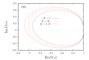
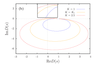
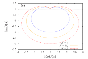
Figure 9: Nyquist diagrams for (a) the Kuramoto model with $(\gamma_{1},\Omega)=(0.6,0.6)$ and $K_{\rm c}\simeq 1.084618$, (b) the Sakaguchi-Kuramoto model with $(\gamma_{1},\Omega)=(0.25,0)$, $\alpha=-1.436475$ and $K_{\rm c}\simeq 1.821283$, and (c) the frequency-weighted-coupling model with $(\gamma_{1},\Omega)=(0.25,0)$ and $K_{\rm c}=5$. In each panel three curves are shown for $K<K_{\rm c}$ (blue broken), $K=K_{\rm c}$ (orange solid), and $K>K_{\rm c}$ (red dot-dashed). The inset of (b) is a magnification around the origin.

Appendix E Divergence condition in the Kuramoto model with symmetric unimodal distributions

Here, we show that in the Kuramoto model with symmetric unimodal natural frequency distributions the divergence condition $\mathrm{Im}\,F\left(\omega_{\text{ex}}\right)=0$ holds if and only if $\omega_{\text{ex}}=\Omega$, where $\Omega$ is the mode of $g(\omega)$. We consider $g_{0}(\omega-\Omega)=g(\omega)$, so that $g_{0}(\omega)$ is even unimodal distribution. Then, the shifted distribution $g(\omega+\Omega)$ is even.

We consider the shift of $g(\omega)$ as $g(\omega+\omega_{\rm ex})=g_{0}(\omega+a)$ where $a=\omega_{\rm ex}-\Omega$ and discuss the function

$$G={\rm PV}\int_{-\infty}^{\infty}d\omega\dfrac{g(\omega+\omega_{\rm ex})}{\omega}={\rm PV}\int_{-\infty}^{\infty}d\omega\dfrac{g_{0}(\omega+a)}{\omega}.$$ (88)

From the definition of the even function $a=0$ implies $G=0$. We show that $G=0$ implies $a=0$ through the contraposition: $a\neq 0$ implies $G\neq 0$.

Changing the variable $\omega$ to $-\omega$, the integral is also written as

$$G=-{\rm PV}\int_{-\infty}^{\infty}d\omega\dfrac{g_{0}(\omega-a)}{\omega}.$$ (89)

We may therefore assume $a>0$ to prove $G\neq 0$ without loss of generality. Adding the two expressions, we have

$$\begin{split}2G&={\rm PV}\int_{-\infty}^{\infty}d\omega\dfrac{g_{0}(\omega+a)-g_{0}(\omega-a)}{\omega}\\ &=\lim_{\epsilon\to+0}(G^{+}+G^{-})\end{split}$$ (90)

where

$$\begin{split}&G^{+}=\int_{\epsilon}^{\infty}d\omega\dfrac{g_{0}(\omega+a)-g_{0}(\omega-a)}{\omega},\\ &G^{-}=\int_{-\infty}^{-\epsilon}d\omega\dfrac{g_{0}(\omega+a)-g_{0}(\omega-a)}{\omega}.\\ \end{split}$$ (91)

From the identity

$$(\omega+a)^{2}-(\omega-a)^{2}=4\omega a,$$ (92)

we can find

$$\left\{\begin{array}[]{ll}|\omega+a|>|\omega-a|&(\text{for }\omega>0),\\ |\omega+a|<|\omega-a|&(\text{for }\omega<0).\\ \end{array}\right.$$ (93)

Further, from the unimodality of $g_{0}$, we have

$$|x|>|y|\quad\Longrightarrow\quad g_{0}(x)<g_{0}(y).$$ (94)

Putting all together, we have $G^{+}<0$ and $G^{-}<0$, and hence $G<0$.

References

- (1) Y. Kuramoto, Self-entrainment of a population of coupled non-linear oscillators, Int. Symp. on Mathematical Problems in Theoretical Physics (Springer, New York, 1975), pp.420-2.
- (2) Y. Kuramoto, Chemical oscillations, waves, and turbulence, (Dover, New York, 2003).
- (3) S. H. Strogatz, From Kuramoto to Crawford: exploring the onset of synchronization in populations of coupled oscillators, Physica D 143 (2000): 1-20.
- (4) Y. Kuramoto, Cooperative dynamics of oscillator community, Prog. Theor. Phys. Suppl. 79, 223 (1984).
- (5) E. A. Martens, E. Barreto, S. H. Strogatz, E. Ott, P. So and T. M. Antonsen, Exact results for the Kuramoto model with a bimodal frequency distribution, Phys. Rev. E 79, 026204 (2009).
- (6) D. Pazó and E. Montbrió, Existence of hysteresis in the Kuramoto model with bimodal frequency distributions, Phys. Rev. E 80, 046215 (2009).
- (7) L. Basnarkov and V. Urumov, Phase transitions in the Kuramoto model, Phys. Rev. E 76, 057201 (2007).
- (8) L. Basnarkov and V. Urumov, Kuramoto model with asymmetric distribution of natural frequencies, Phys. Rev. E 78, 011113 (2008).
- (9) Y. Terada, K. Ito, T. Aoyagi and Y. Y. Yamaguchi, Nonstandard transitions in the Kuramoto model: a role of asymmetry in natural frequency distributions, J. Stat. Mech. (2017) 013403.
- (10) O. E. Omel’chenko and M. Wolfrum, Nonuniversal transitions to synchrony in the Sakaguchi-Kuramoto model, Phys. Rev. Lett. 109, 164101 (2012).
- (11) O. E. Omel’chenko and M. Wolfrum, Bifurcations in the Sakaguchi-Kuramoto model, Physica D 263, 74-85 (2013).
- (12) W. Zhou, L. Chen, H. Bi, X. Hu, Z. Liu and S. Guan, Explosive synchronization with asymmetric frequency distribution, Phys. Rev. E 92 012812 (2015).
- (13) T. Qiu, Y. Zhang, J. Liu, H. Bi, S. Boccaletti, Z. Liu and S. Guan, Landau damping effects in the synchronization of conformist and contrarian oscillators, Sci. Rep. 5, 18235 (2015).
- (14) C. Xu, J. Gao, H. Xiang, W. Jia, S. Guan and Z. Zheng, Dynamics of phase oscillators with generalized frequency-weighted coupling, Phys. Rev. E 94, 062204 (2016).
- (15) Y. Xiao, W. Jia, C. Xu, H. Lu and Z. Zheng, Synchronization of phase oscillators in the generalized Sakaguchi-Kuramoto model, Europhys. Lett. 118 60005 (2017).
- (16) H. Sakaguchi, Cooperative Phenomena in Coupled Oscillator Systems under External Fields, Prog. Theor. Phys. 79, 39 (1988).
- (17) H. Daido, Susceptibility of large populations of coupled oscillators, Phys. Rev. E 91, 012925 (2015).
- (18) A. Patelli, S. Gupta, C. Nardini and S. Ruffo, Linear response theory for long-range interacting systems in quasistationary states, Phys. Rev. E 85, 021133 (2012).
- (19) S. Ogawa and Y. Y. Yamaguchi, Linear response theory in the Vlasov equation for homogeneous and for inhomogeneous quasistationary states, Phys. Rev. E 85, 061115 (2012).
- (20) M. Komarov and A. Pikovsky, Multiplicity of Singular Synchronous States in the Kuramoto Model of Coupled Oscillators, Phys. Rev. Lett. 111, 204101 (2013).
- (21) M. Komarov and A. Pikovsky, The Kuramoto model of coupled oscillators with a bi-harmonic coupling function, Physica D 289, 18-31 (2014).
- (22) K. Li, S. Ma, H. Li and J. Yang, Transition to synchronization in a kuramoto model with the first- and second-order interaction terms, Phys. Rev. E 89, 032917 (2014).
- (23) F.C. Hoppensteadt, and E.M. Izhikevich, Weakly connected neural networks, (Springer-Verlag, New York, 2012).
- (24) H. Nakao, Phase reduction approach to synchronisation of nonlinear oscillators, Contemp. Phys. 57, 188 (2016).
- (25) P. Dayan and L.F. Abbott, Theoretical neuroscience, (MIT Press, Cambridge, 2001).
- (26) H. Hong and S. H. Strogatz, Kuramoto Model of Coupled Oscillators with Positive and Negative Coupling Parameters: An Example of Conformist and Contrarian Oscillators, Phys. Rev. Lett. 106, 054102 (2011).
- (27) H. Sakaguchi and Y. Kuramoto, A soluble active rotator model showing phase transitions via mutual entrainment, Prog. Theor. Phys. 76, 576 (1986).
- (28) G. H. Paissan and D. H. Zanette, Synchronization of phase oscillators with heterogeneous coupling: A solvable case, Physica D 237, 818 (2008).
- (29) D. Iatsenko, S. Petkoski, P.V.E. McClintock and A. Stefanovska, Stationary and TravelingWave States of the Kuramoto Model with an Arbitrary Distribution of Frequencies and Coupling Strengths, Phys. Rev. Lett. 110, 064101 (2013).
- (30) H. Daido, Population Dynamics of Randomly Interacting Self-Oscillators. I -Tractable Models without Frustration, Prog. Theor. Phys. 77, 622 (1987).
- (31) C. Lancellotti, On the vlasov limit for systems of nonlinearly coupled oscillators without noise, Transp. Theory Stat. Phys. 34, 523.
- (32) E. Ott, and T.M. Antonsen, Low dimensional behavior of large systems of globally coupled oscillators, Chaos 18, 037113 (2008).
- (33) E. Ott, and T.M. Antonsen, Long time evolution of phase oscillator systems, Chaos 19, 023117 (2009).
- (34) H. Hong, H. Chaté, L.-H. Tang and H. Park, Finite-size scaling, dynamic fluctuations, and hyperscaling relation in the Kuramoto model, Phys. Rev. E 92, 022122 (2015).