Multi-Scale Spectrum Sensing in
Dense Multi-Cell Cognitive Networks

Abstract

Multi-scale spectrum sensing is proposed to overcome the cost of full network state information on the spectrum occupancy of primary users (PUs) in dense multi-cell cognitive networks. Secondary users (SUs) estimate the local spectrum occupancies and aggregate them hierarchically to estimate spectrum occupancy at multiple spatial scales. Thus, SUs obtain fine-grained estimates of spectrum occupancies of nearby cells, more relevant to scheduling tasks, and coarse-grained estimates of those of distant cells. An agglomerative clustering algorithm is proposed to design a cost-effective aggregation tree, matched to the structure of interference, robust to local estimation errors and delays. Given these multi-scale estimates, the SU traffic is adapted in a decentralized fashion in each cell, to optimize the trade-off among SU cell throughput, interference caused to PUs, and mutual SU interference. Numerical evaluations demonstrate a small degradation in SU cell throughput (up to 15% for a 0dB interference-to-noise ratio experienced at PUs) compared to a scheme with full network state information, using only one-third of the cost incurred in the exchange of spectrum estimates. The proposed interference-matched design is shown to significantly outperform a random tree design, by providing more relevant information for network control, and a state-of-the-art consensus-based algorithm, which does not leverage the spatio-temporal structure of interference across the network.

I Introduction

The recent proliferation of mobile devices has been exponential in number as well as heterogeneity [4], demanding new tools for the design of agile wireless networks [5]. Fifth-generation (5G) cellular systems will meet this challenge in part by deploying dense, heterogeneous networks, which must flexibly adapt to time-varying network conditions. Cognitive radios [6] have the potential to improve spectral efficiency by enabling secondary users (SUs) to exploit resource gaps left by legacy primary users (PUs) [7]. However, estimating these resource gaps in real-time becomes increasingly challenging with the increasing network densification, due to the signaling overhead required to learn the network state [8]. Furthermore, network densification results in irregular network topologies. These features demand effective interference management to fully leverage spatio-temporal spectrum access opportunities.

To meet this challenge, we develop and analyze spectrum utilization and interference management techniques for dense cognitive radios with irregular interference patterns. We consider a multi-cell network with a set of PUs and a dense set of opportunistic SUs, which seek access to locally unoccupied spectrum. The SUs must estimate the channel occupancy of the PUs across the network based on local measurements. In principle, these measurements can be collected at a fusion center [9, 10, 11], but centralized estimation may incur unacceptable delays and overhead [12, 8]. To reduce this cost and provide a form of coordination, neighboring cells may inform each other of spectrum they are occupying [13]; however, this scheme cannot manage interference beyond the cell neighborhood, which may be significant in dense topologies.

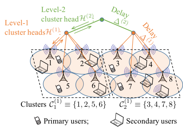
Figure 1: System model (see notation in Sec. III).

We address this challenge by designing a cost-effective multi-scale solution to detect and leverage spatio-temporal spectrum access opportunities across the network, by exploiting the structure and irregularities of interference. To do so, note that the interference caused by a given SU depends on its position in the network, as depicted in Fig. 1: PUs closer to this SU will experience stronger interference than PUs farther away. Therefore, such SU should estimate more accurately the state of nearby PUs, in order to perform more informed local control decisions to access the spectrum or remain idle. In contrast, the state of PUs farther away, which experience less interference from such SU, is less relevant to these control decisions, hence coarser spectrum estimates may suffice. With this in mind, the goal of our formulation is the design of a cost-effective spectrum sensing architecture to aid local network control, which enables each SU to estimate the spectrum occupancy at different spatial scales (hence the name "multi-scale"), so as to possess an accurate and fine-grained estimate of the occupancy of PUs in the vicinity, and coarser estimates of the occupancy states of PUs farther away. To achieve this goal, we use a hierarchical estimation approach resilient to delays and errors in the information exchange and estimation processes, inspired by [14] in the context of averaging consensus [15]: local measurements are fused hierarchically up a tree, which provides aggregate spectrum occupancy information for clusters of cells at larger and larger scales. Thus, SUs acquire precise information on the spectrum occupancies of nearby cells – these cells are more susceptible to interference caused by nearby SUs – and coarse, aggregate information on the occupancies of faraway cells. By generating spectrum occupancy estimates at multiple spatial scales (i.e., multi-scale), this scheme permits an efficient trade-off of estimation quality, cost of aggregation, estimation delay, and provides a cost-effective means to acquire information most relevant to network control. We derive the ideal estimator of the global spectrum occupancy from the multi-scale measurements, and we design the SU traffic in each cell in a decentralized fashion so as to maximize a trade-off among SU cell throughput, interference caused to PUs, and mutual SU interference.

To tailor the aggregation tree to the interference pattern of the network, we design an agglomerative clustering algorithm [16, Ch. 14]. We measure the end-to-end performance in terms of the trade-off among SU cell throughput, interference to PUs, and the cost efficiency of aggregation. We show numerically that our design achieves a small degradation in SU cell throughput (up to 15% under a reference interference-to-noise ratio of 0dB experienced at PUs) compared to a scheme with full network state information, while incurring only one-third of the cost in the aggregation of spectrum estimates across the network. We show that the proposed interference-matched tree design based on agglomerative clustering significantly outperforms a random tree design, thus demonstrating that it provides more relevant information for network control. Finally, we compare our proposed design with the state-of-the-art consensus-based algorithm [17], originally designed for single-cell systems without temporal dynamics in the PU spectrum occupancy, and we demonstrate the superiority of our scheme thanks to its ability to leverage the spatial and temporal dynamics of interference in the network and to provide more meaningful information for network control.

Related work: Consensus-based schemes for spectrum estimation have been proposed in [17, 18, 8, 19]: [8] proposes a mechanism to select only the SUs with the best detection performance to reduce the overhead of spectrum sensing; while [19] focuses on the design of diffusion methods. Cooperative schemes with data fusion have been proposed in [9, 10, 11]: [9] investigates the optimal voting rule and optimal detection threshold; [10] proposes a robust scheme to filter out abnormal measurements, such as malicious or unreliable sensors; [11] analyses and compares hard and soft combining schemes in heterogeneous networks. However, all these works focus on a scenario with a single PU pair (one cell) and no temporal dynamics in the PU spectrum occupancy state. Instead, we investigate spectrum sensing in multi-cell networks with multiple PU pairs and with temporal dynamics in the PU occupancy state, giving rise to both spatial and temporal spectrum access opportunities. Similar opportunities have been explored in [20], but in the context of a single PU, and without consideration of SU scheduling decisions. In contrast, in our paper we investigate the impact of spectrum sensing on scheduling decisions of SUs.

Another important difference with respect to [17, 18, 8, 19, 9] (with the exception of [20]) is that we model temporal dynamics in the occupancy states of each PU, as a result of PUs joining and leaving the network at random times; in time-varying settings, the performance of spectrum estimation may be severely affected by delays in the propagation of estimates across the network, so that spectrum estimates may become outdated. We develop a hierarchical estimation approach that compensates for these propagation delays. A setting with temporal dynamics has been proposed in [21, 20] for a single-cell system, but without consideration of delays.

Finally, [22] capitalizes on sparsity due to the narrow-band frequency use, and to sparsely located active radios, and develops estimators to enable identification of the (un)used frequency bands at arbitrary locations; differently from this work, we develop techniques to track the activity of PUs, and use this information to schedule transmissions of SUs, hence we investigate the interplay between estimation and scheduling tasks, and the role of network state information.

We summarize the contributions of this paper as follows:

1. We propose a hierarchical framework to aggregate network state information (NSI) over a multi-cell wireless network, with a generic interference pattern among cells, which enables spectrum estimation at multiple spatial scales, most informative to network control. We study its performance in terms of the trade-off between the SU cell throughput and the interference caused to the PUs. We design the optimal SU traffic in each cell in a decentralized fashion, so as to manage the interference caused to other PUs and SUs.

2. We show that the belief of the spectrum occupancy vector is statistically independent across subsets of cells at different spatial scales, and uniform within each subset (Theorem 1), up to a correction factor that accounts for mismatches in the aggregation delays. This result greatly facilitates the estimation of the interference caused to PUs (Lemma 3).

3. We address the design of the hierarchical aggregation tree under a constraint on the aggregation cost based on agglomerative clustering [16, Ch. 14] (Algorithm 1).

Our analysis demonstrates that multi-scale spectrum estimation using hierarchical aggregation matched to the structure of interference is a much more cost-effective solution than fine-grained network state estimation, and provides more valuable information for network control. Additionally, it demonstrates the importance of leveraging the spatial and temporal dynamics of interference arising in dense multi-cell systems, made possible by our multi-scale strategy; in contrast, consensus-based strategies, which average out the spectrum estimate over multiple cells and over time, are unable to achieve this goal and perform poorly in dense multi-cell systems.

This paper is organized as follows. In Sec. II, we present the system model. In Sec. III, we present the proposed local and multi-scale estimation algorithms, whose performance is analyzed in Sec. IV. In Sec. V, we address the tree design. In Sec. VI, we present numerical results and, in Sec. VII, we conclude this paper. The main proofs are provided in the Appendix. Table I provides the main parameters and metrics.

$\mathcal{C}$	set of cells, with $|\mathcal{C}|=N_{C}$	$b_{i,t}$	occupancy state of cell $i$ at time $t$, ${\in}\{0,1\}$
$\pi_{B}$	steady-state distribution $\mathbb{P}(b_{i,t}=1)$	$\mu$	memory of the Markov chain $\{b_{i,t},t\geq 0\}$
$\phi_{i,j}$	INR generated by tx in cell $i$ to rx in $j$, cf. (II)	$a_{i,t}$	SU traffic in cell $i$ at time $t$, ${\in}[0,M_{i,t}]$
$M_{i,t}$	# of SUs in cell $i$ at time $t$	$\mathcal{B}_{N}(p)$	Binomial with $N$ trials and probability $p$
$\mathcal{H}^{(L)}$	level-$L$ cluster heads	$\mathcal{H}_{m}^{(L)}$	level-$L$ cluster heads associated to $m{\in}\mathcal{H}^{(L+1)}$
$\mathcal{C}_{k}^{(L)}$	cells associated to $k\in\mathcal{H}^{(L)}$	$\Lambda_{i,j}$	h-distance between cells $i$ and $j$, cf. Def. 1
		$\mathcal{D}_{i}^{(L)}$	cells at h-distance $L$ from cell $i$, cf. Def. 2
$\delta_{i}^{(L)}$	delay from cell $i$ to level-$L$ cluster head	$\Delta_{m}^{(L)}$	delay between $m{\in}\mathcal{H}_{n}^{(L-1)}$
			and its upper level-$L$ cluster head $n$
$\hat{b}_{i,t}$	local estimate at cell $i$	$\sigma_{i,t}^{(L)}$	delay mismatched aggregate estimate at
			h-distance $L$ from cell $i$, cf. (27)
$\hat{r}_{i,t}$	SU cell $i$ throughput lower bound, cf. (II)	$I_{S,i}(t)$	estimated SU interference at cell $i$, cf. (8)
$\iota_{P,i}$	INR caused by SUs in cell $i$, cf. (11)-(12)	$I_{P,i}$	estimated PU interference at cell $i$, cf. (9)
$u_{i,t}$	utility function, cf. (II)	$\pi_{i,t}$	local belief in cell $i$

TABLE I: Table of Notation

II System Model

Network Model: We consider the network depicted in Fig. 1, composed of a multi-cell network of PUs with $N_{C}$ cells operating in downlink, indexed by $\mathcal{C}{\equiv}\{1,2,\dots,N_{C}\}$, and an unlicensed network of SUs. The receivers are located in the same cell as their transmitters, so that they receive from the closest access point. Transmissions are slotted and occur over frames. Let $t$ be the frame index, and $b_{i,t}{\in}\{0,1\}$ be the PU spectrum occupancy of cell $i{\in}\mathcal{C}$ during frame $t$, with $b_{i,t}{=}1$ if occupied and $b_{i,t}{=}0$ otherwise. We suppose that $\{b_{i,t},t\geq 0,i\in\mathcal{C}\}$ are independent and identically distributed (i.i.d.) across cells and evolve according to a two-state Markov chain, as a result of PUs joining and leaving the network at random times. We define the transition probabilities as

$\nu_{1}\triangleq\mathbb{P}(b_{i,t+1}{=}1|b_{i,t}{=}0),\ \nu_{0}\triangleq\mathbb{P}(b_{i,t+1}{=}0|b_{i,t}{=}1),$

where $\mu{\triangleq}1{-}\nu_{1}{-}\nu_{0}$ is the memory of the Markov chain, which dictates the rate of convergence to its steady-state distribution. Hence, $\pi_{B}{\triangleq}\mathbb{P}(b_{i,t}=1){=}\frac{\nu_{1}}{1{-}\mu}$ at steady-state. We denote the state of the network at time $t$ as $\mathbf{b}_{t}=(b_{1,t},b_{2,t},\dots,b_{N_{C},t})$.
We assume that PUs and SUs coexist in the same spectrum band. Let $M_{i,t}$ be the number of SUs in cell $i$ at time $t$, which may vary over time as a result of SUs joining and leaving the network. We collect $M_{i,t}$ in the vector $\mathbf{M}_{t}$.

Assumption 1.

$\{\mathbf{M}_{t}{,}t{\geq}0\}$ are i.i.d. across cells, stationary and independent of $\{\mathbf{b}_{t}{,}t{\geq}0\}$, that is

$$\mathbb{P}\bigl{(}\mathbf{b}_{t}{=}\tilde{\mathbf{b}}_{t},\mathbf{M}_{t}{=}\tilde{\mathbf{M}}_{t},\forall t\in\mathcal{T}\bigr{)}=\prod_{i}\mathbb{P}\bigl{(}b_{i,t}{=}\tilde{b}_{i,t},t{\in}\mathcal{T}\bigr{)}$$

$$\qquad\times\mathbb{P}\bigl{(}M_{i,t}{=}\tilde{M}_{i,t},t{\in}\mathcal{T}\bigr{)}\ \text{ (independence),}$$

$$\mathbb{P}\bigl{(}M_{i,t}{=}\tilde{M}_{i,t},t{\in}\mathcal{T}\bigr{)}{=}\mathbb{P}\bigl{(}M_{i,t-\delta}{=}\tilde{M}_{i,t},t{\in}\mathcal{T}\bigr{)}\ \text{ (stationarity).}$$

where $\mathcal{T}$ is a time interval and $\delta>0$ is a delay. Additionally, $M_{i,t}>0,\forall i,t$ (dense network).∎

Assumption 1 guarantees that spectrum estimates are “statistically symmetric” [23], i.e., they exhibit the same statistical properties at different cells and delay scales. An example which obeys Assumption 1 is when $M_{i,t}$ is a Markov chain taking values from $M_{i,t}>0$, i.i.d. across cells. The SUs opportunistically access the spectrum to maximize their own cell throughput, while at the same time limiting the interference caused to other SUs and to the PUs. Their access decision is governed by the local SU access traffic $a_{i,t}{\in}[0,M_{i,t}]$ for SUs in cell $i$. We assume an uncoordinated SU access strategy so that, given $a_{i,t}$, all the $M_{i,t}$ SUs in cell $i$ access the channel with probability $a_{i,t}/M_{i,t}$, independently of each other. Therefore, $a_{i,t}$ represents the expected number of SU transmissions in cell $i$. We let $\mathbf{a}_{t}{=}(a_{1,t},a_{2,t},\dots,a_{N_{C},t})$.
Transmissions of SUs and PUs generate interference to each other. We denote the interference to noise ratio (INR) generated by the activity of a transmitter in cell $i$ to a receiver in $j$ as $\phi_{i,j}{\geq}0$, collected into the symmetric (due to channel reciprocity) matrix $\bm{\Phi}{\in}\mathbb{R}^{N_{C}\times N_{C}}$. Typically,

$$[\phi_{i,j}]_{\mathrm{dB}}=[P_{tx}]_{\mathrm{dBm}}-[N_{0}W_{tot}]_{\mathrm{dBm}}$$

$$\qquad-[L_{ref}]_{\mathrm{dB}}-\alpha_{i,j}[d_{i,j}/d_{ref}]_{\mathrm{dB}}$$ (1)

(see, e.g., [24]), where $P_{tx}$ is the transmission power, common to all PUs and SUs, $N_{0}$ is the noise power spectral density and $W_{tot}$ is the signal bandwidth; $L_{ref}$ is the large-scale pathloss at a reference distance $d_{ref}$, based on Friis’ free space pathloss formula, and $[d_{i,j}/d_{ref}]^{\alpha_{i,j}}$ is the distance dependent component, with $d_{i,j}$ and $\alpha_{i,j}$ the distance and pathloss exponent between cells $i$ and $j$. We assume that the intended receiver of each PU or SU transmission is located within the cell radius, so that $\phi_{i,i}$ is the SNR to the intended receiver in cell $i$. In practice, the large-scale pathloss exhibits variations as transmitter or receiver are moved within the cell coverage. Thus, $\phi_{i,j}$ can be interpreted as an average of these pathloss variations, or a low resolution approximation of the large-scale pathloss map. This is a good approximation due to the small cell sizes arising in dense cell deployments, as considered in this paper. In Sec. VI (Fig. 5), we will demonstrate its robustness in a more realistic setting.
Network Performance Metrics: We label each SU as $(j,n)$, denoting the $n$th SU in cell $j$. Let $v_{j,n,t}\in\{0,1\}$ be the indicator of whether SU $(j,n)$ transmits based on the probabilistic access decision outlined above; this is stacked in the vector $\mathbf{v}_{t}$. If the reference SU $(i,1)$ transmits, the signal received by the corresponding SU receiver is

$$y_{i,1}(t)=\sqrt{\phi_{i,i}}h_{i,1}^{(s)}(t)x_{i,1}^{(s)}(t)+{w_{i,1}(t)}+n_{i,1}(t),$$ (2)

where we have defined the interference signal

$$w_{i,1}(t)\triangleq \sum_{(j,n)\neq(i,1)}\sqrt{\phi_{j,i}}h_{j,n}^{(s)}(t)v_{j,n,t}x_{j,n}^{(s)}(t)$$

$$+\sum_{j=1}^{N_{C}}\sqrt{\phi_{j,i}}h_{j}^{(p)}(t)b_{j,t}x_{j}^{(p)}(t),$$ (3)

$h_{j,n}^{(s)}(t)$ is the fading channel between SU $(j,n)$ and the reference SU $(i,1)$, with $x_{j,n}^{(s)}(t)$ the unit energy transmitted signal; $h_{j}^{(p)}(t)$ is the fading channel between PU $j$ (transmitting in downlink) and SU $(i,1)$, with $x_{j}^{(p)}(t)$ the unit energy transmitted signal; $\phi_{j,i}$ is the large-scale pathloss between cells $j$ and $i$, see (II); $n_{i,1}(t){\sim}\mathcal{CN}(0,1)$ is circular Gaussian noise; we assume Rayleigh fading, so that $h_{j,n}^{(s)}(t),h_{j}^{(p)}(t)\sim\mathcal{CN}(0,1)$. The transmission is successful if and only if the SINR exceeds a threshold $\mathrm{SINR}_{\mathrm{th}}$; we then obtain the success probability of SU $(i,1)$, conditional on $\mathbf{v}_{t}$ and $\mathbf{b}_{t}$,

$$\rho_{i,1}(\mathbf{v}_{t},\mathbf{b}_{t})=\mathbb{P}\left(\left.\frac{\phi_{i,i}|h_{i,1}^{(s)}(t)|^{2}}{1+\left|w_{i,1}(t)\right|^{2}}>\mathrm{SINR}_{\mathrm{th}}\right|\mathbf{v}_{t},\mathbf{b}_{t}\right).$$ (4)

Noting that $w_{i,1}(t)|(\mathbf{v}_{t},\mathbf{b}_{t})$ is circular Gaussian with zero mean and variance

$$\mathbb{E}[|w_{i,1}(t)|^{2}|\mathbf{v}_{t},\mathbf{b}_{t}]\triangleq\sum_{j=1}^{N_{C}}\phi_{j,i}\eta_{j}+\sum_{j=1}^{N_{C}}\phi_{j,i}b_{j,t}-\phi_{i,i},$$ (5)

where $\eta_{j}\triangleq\sum_{n=1}^{M_{j,t}}v_{j,n,t}$ is the number of SUs that attempt spectrum access in cell $j$, we obtain

$$\rho_{i}(\mathbf{v}_{t},\mathbf{b}_{t}){=}\frac{e^{-\mathrm{SINR}_{\mathrm{th}}/\phi_{i,i}}}{1+\mathrm{SINR}_{\mathrm{th}}\left[\sum_{j=1}^{N_{C}}\frac{\phi_{j,i}}{\phi_{i,i}}\eta_{j}+\sum_{j=1}^{N_{C}}\frac{\phi_{j,i}}{\phi_{i,i}}b_{j,t}-1\right].}$$

Then, the throughput in cell $i$, conditional on the SU traffic $\mathbf{a}_{t}$ and PU network state $\mathbf{b}_{t}$, is obtained by noting that each of the $\eta_{i}$ SUs succeed with probability $\rho_{i}$; hence, taking the expectation with respect to the number of SUs performing spectrum access, $\eta_{j}{\sim}\mathcal{B}_{M_{j,t}}(a_{j,t}/M_{j,t})$ (binomial random variable with probability $a_{j,t}/M_{j,t}$ and $M_{j,t}$ trials), we obtain

$$r_{i,t}(\mathbf{a}_{t},\mathbf{b}_{t})$$ (6)

$${\triangleq}\mathbb{E}_{\eta}\left[\left.\frac{\eta_{i}\exp\left\{-\frac{1}{\phi_{i,i}}\mathrm{SINR}_{\mathrm{th}}\right\}}{1{+}\mathrm{SINR}_{\mathrm{th}}\left[\sum_{j=1}^{N_{C}}\frac{\phi_{j,i}}{\phi_{i,i}}\eta_{j}{-}1{+}\sum_{j=1}^{N_{C}}\frac{\phi_{j,i}}{\phi_{i,i}}b_{j,t}\right]}\right|\mathbf{a}_{t},\mathbf{b}_{t}\right]$$

$${=}\mathbb{E}_{\eta,\hat{\eta}_{i}}\left[\left.\frac{a_{i,t}\exp\left\{-\frac{1}{\phi_{i,i}}\mathrm{SINR}_{\mathrm{th}}\right\}}{1{+}\mathrm{SINR}_{\mathrm{th}}\left[\hat{\eta}_{i}{+}\sum_{j\neq i}\frac{\phi_{j,i}}{\phi_{i,i}}\eta_{j}{+}\sum_{j=1}^{N_{C}}\frac{\phi_{j,i}}{\phi_{i,i}}b_{j,t}\right]}\right|\mathbf{a}_{t},\mathbf{b}_{t}\right],$$

where the second equality is obtained by the change of variable $\hat{\eta}_{i}{=}\eta_{i}{-}1$, with $\hat{\eta}_{i}{\sim}\mathcal{B}(a_{i,t}/M_{i,t},M_{i,t}{-}1)$. The computation of the SU cell throughput using this formula has high complexity, due to the outer expectation. Therefore, we resort to a lower bound. Noting that the argument of the expectation is a convex function of $\eta_{j},\forall j$ and $\hat{\eta}_{i}$, Jensen’s inequality yields

$$r_{i,t}(\mathbf{a}_{t},\mathbf{b}_{t}){\geq} \frac{a_{i,t}\exp\left\{-\frac{1}{\phi_{i,i}}\mathrm{SINR}_{\mathrm{th}}\right\}}{1{+}\mathrm{SINR}_{\mathrm{th}}\sum_{j=1}^{N_{C}}\frac{\phi_{j,i}}{\phi_{i,i}}(a_{j,t}+b_{j,t}){-}\mathrm{SINR}_{\mathrm{th}}\frac{a_{i,t}}{M_{i,t}}}.$$

Cell $i$ selects $a_{i,t}$ based on partial NSI, denoted by the local belief $\pi_{i,t}(\mathbf{b})$ that $\mathbf{b}_{t}{=}\mathbf{b}$. Taking the expectation over $\mathbf{b}_{t}$ conditional on $\pi_{i,t}$ and using Jensen’s inequality, we obtain

$$\mathbb{E}\left[r_{i,t}(\mathbf{a}_{t},\mathbf{b}_{t})|\pi_{i,t}\right]$$

$$\geq\frac{a_{i,t}\exp\left\{-\frac{1}{\phi_{i,i}}\mathrm{SINR}_{\mathrm{th}}\right\}}{1+\mathrm{SINR}_{\mathrm{th}}\left[a_{i,t}(1-M_{i,t}^{-1})+I_{P,i}(\pi_{i,t})+I_{S,i}(t)\right]}$$

$$\triangleq\hat{r}_{i,t}(a_{i,t},I_{P,i}(\pi_{i,t})),$$ (7)

where we have defined

$$I_{S,i}(t)\triangleq\sum_{j\neq i}\frac{\phi_{j,i}}{\phi_{i,i}}a_{j,t},$$ (8)

$$I_{P,i}(\pi_{i,t}){\triangleq}\mathbb{E}\left[\left.\sum_{j=1}^{N_{C}}\frac{\phi_{j,i}}{\phi_{i,i}}b_{j,t}\right|\pi_{i,t}\right]{=}\sum_{j=1}^{N_{C}}\frac{\phi_{j,i}}{\phi_{i,i}}\mathbb{P}\left(b_{j,t}{=}1|\pi_{i,t}\right).$$ (9)

The terms $I_{S,i}(t)$ and $I_{P,i}(\pi_{i,t})$ represent, respectively, an estimate of the interference strength caused by SUs and PUs operating in the rest of the network to the reference SU in cell $i$. Additionally, due to channel reciprocity and the resulting symmetry on $\bm{\Phi}$, $I_{P,i}(\pi_{i,t})$ represents an estimate of the interference strength caused by the reference SU to the rest of the PU network.

Herein, we use $\hat{r}_{i,t}$ in (II) to characterize the performance of the SUs. Since this is a lower bound to the actual SU cell throughput, using $\hat{r}_{i,t}$ as a metric provides performance guarantees. Note that the performance depends upon the network-wide SU activity $\mathbf{a}_{t}$ via $I_{S,i}(t)$; in turn, each $a_{j,t}$ is decided based on the local belief $\pi_{j,t}$, which may be unknown to the SUs in cell $i$ (which operate under a different belief $\pi_{i,t}$). Therefore, maximization of $\hat{r}_{i,t}(a_{i,t},I_{P,i}(\pi_{i,t}))$ can be characterized as a decentralized decision problem, which does not admit polynomial time algorithms [25]. To achieve low computational complexity, we relax the decentralized decision process by assuming that $I_{S,i}(t)$ is known to cell $i$ in slot $t$. This assumption is based on the following practical arguments: due to the Markov chain dynamics of $\mathbf{b}_{t}$, $\mathbf{a}_{t}$ varies slowly over time, hence $I_{S,i}(t)$ can be estimated by averaging the SU traffic over time; additionally, the spatial variations of $\mathbf{a}_{t}$ are averaged out in the spatial domain since $I_{S,i}(t)$ is a weighted sum of $a_{j,t}$ across cells, yielding slow variations on $I_{S,i}(t)$ due to mean-field effects. In Sec. IV, we will present an approach to estimate $I_{S,i}(t)$ and $I_{P,i}(\pi_{i,t})$ based on hierarchical information exchange over the SU network.

We define the average INR experienced by the PUs as a result of the activity of the SUs as

$$\mathrm{INR}(\mathbf{a}_{t},\mathbf{b}_{t})\triangleq\frac{1}{N_{C}\pi_{B}}\sum_{j=1}^{N_{C}}\sum_{i=1}^{N_{C}}a_{i,t}\phi_{i,j}b_{j,t},$$ (10)

where $N_{C}\pi_{B}$ is the average number of active PUs at steady-state. In fact, the expected number of SUs transmitting in cell $i$ is $a_{i,t}$, so that $a_{i,t}\phi_{i,j}$ is the overall interference caused by SUs in cell $i$ to the PU in cell $j$. $\mathrm{INR}(\mathbf{a}_{t},\mathbf{b}_{t})$ is then obtained by averaging this effect over the network. Herein, we isolate the contribution due to the SUs in cell $i$ on (10), yielding

$$\iota_{P,i}(a_{i,t},\mathbf{b}_{t})\triangleq\frac{1}{\pi_{B}}a_{i,t}\sum_{j=1}^{N_{C}}\phi_{i,j}b_{j,t},$$ (11)

so that $\mathrm{INR}(\mathbf{a}_{t},\mathbf{b}_{t})\triangleq\frac{1}{N_{C}}\sum_{i=1}^{N_{C}}\iota_{P,i}(a_{i,t},\mathbf{b}_{t})$. By computing the expectation with respect to the local belief $\pi_{i,t}$ and using the symmetry of $\bm{\Phi}$, we then obtain

$$\iota_{P,i}(a_{i,t},I_{P,i}(\pi_{i,t})) \triangleq\mathbb{E}[\iota_{P,i}(a_{i,t},\mathbf{b}_{t})|\pi_{i,t}]$$

$$=\frac{1}{\pi_{B}}a_{i,t}\phi_{i,i}I_{P,i}(\pi_{i,t}).$$ (12)

Since the goal of SUs is to maximize their own cell throughput, while minimizing their interference to the PUs, we define the local utility as a payoff minus cost function,

$$u_{i,t}(a_{i,t},I_{P,i}(\pi_{i,t}))$$

$$\triangleq\hat{r}_{i,t}(a_{i,t},I_{P,i}(\pi_{i,t}))-\lambda\iota_{P,i}(a_{i,t},I_{P,i}(\pi_{i,t})),$$ (13)

where $\lambda{>}0$ is a cost parameter which balances the two competing goals. Given $\pi_{i,t}$, the goal of the SUs in cell $i$ is to design $a_{i,t}$ so as to maximize $u_{i,t}(a_{i,t},I_{P,i}(\pi_{i,t}))$. Since this is a concave function of $a_{i,t}$ (as can be seen by inspection), we obtain the optimal SU traffic

$$a_{i,t}^{*}(I_{P,i}(\pi_{i,t}))\triangleq\underset{a_{i,t}\in[0,M_{i,t}]}{\arg\max}u_{i,t}(a_{i,t},I_{P,i}(\pi_{i,t}))$$

$$=\Biggl{[}\frac{\sqrt{1+\mathrm{SINR}_{\mathrm{th}}\left[I_{P,i}(\pi_{i,t})+I_{S,i}(t)\right]}}{\mathrm{SINR}_{\mathrm{th}}(1-1/M_{i,t})}$$ (14)

$${\times}\Biggl{(}\frac{\sqrt{\pi_{B}}e^{-\frac{\mathrm{SINR}_{\mathrm{th}}}{2\phi_{i,i}}}}{\sqrt{\lambda\phi_{i,i}I_{P,i}(\pi_{i,t})}}{-}\sqrt{1{+}\mathrm{SINR}_{\mathrm{th}}\left[I_{P,i}(\pi_{i,t}){+}I_{S,i}(t)\right]}\Biggr{)}\Biggr{]}_{0}^{M_{i,t}},$$

where $[\cdot]_{0}^{m}=\min\{\max\{\cdot,0\},m\}$ denotes the projection operation onto the interval $[0,m]$. It can be shown by inspection that both $a_{i,t}^{*}$ and $u_{i,t}^{*}$ are non-increasing functions of $I_{P,i}(\pi_{i,t})$, so that, as the PU activity increases ($I_{P,i}(\pi_{i,t})$ increases), the SU activity and the local utility both decrease; when $I_{P,i}(\pi_{i,t})$ is above a certain threshold, then $a_{i,t}^{*}=0$ and $u_{i,t}^{*}(I_{P,i}(\pi_{i,t}))=0$; indeed, in this case the PU network experiences high activity, hence SUs remain idle to avoid interfering. Additionally, $u_{i,t}^{*}(I_{P,i}(\pi_{i,t}))$ is a convex function of $I_{P,i}(\pi_{i,t})$. Then, by Jensen’s inequality,

$$u_{i,t}^{*}(I_{P,i}(\pi_{i,t}))\leq\sum_{\mathbf{b}\in\{0,1\}^{N_{C}}}\pi_{i,t}(\mathbf{b})u_{i,t}^{*}(I_{P,i}(\mathcal{I}_{\mathbf{b}})),$$ (15)

where $\mathcal{I}_{\mathbf{b}}$ is the Kronecker delta function centered at $\mathbf{b}$, reflecting the special case when $\mathbf{b}_{t}$ is known, so that $u_{i,t}^{*}(I_{P,i}(\mathcal{I}_{\mathbf{b}}))$ represents the utility achieved when $\mathbf{b}_{t}=\mathbf{b}$, known. Consequently, the expected network utility is maximized when $\mathbf{b}_{t}$ is known (full NSI). Thus, the SUs should, possibly, obtain full NSI in order to achieve the best performance. To approach this goal, the SUs in cell $i$ should obtain $\mathbf{b}_{t}$ in a timely fashion. To this end, the SUs in cell $j{\neq}i$ should report the local and current spectrum state $b_{j,t}$ to the SUs in cell $i$ via information exchange, potentially over multiple hops. Since this needs to be done over the entire network (i.e., for every pair $(i,j)\in\mathcal{C}^{2}$), the associated overhead may be impractical in dense multi-cell network deployments. Additionally, these spectrum estimates may be noisy and delayed, hence they may become outdated and not informative for network control. In order to reduce the overhead of full-NSI, we now develop a scheme to estimate spectrum occupancy based on delayed, noisy, and aggregate (vs timely, noise-free and fine-grained) spectrum measurements over the network.

III Local and Multi-scale Estimation Algorithms

In this section, we propose a method to estimate $I_{P,i}(\pi_{i,t})$ and $I_{S,i}(t)$ at cell $i$ based on hierarchical information exchange. To this end, SUs exchange estimates of the local PU spectrum occupancy $b_{i,t}$, denoted as $\hat{b}_{i,t}$, as well as the local SU traffic decision variable $a_{i,t}$. For conciseness, we will focus on the estimation of $I_{P,i}(\pi_{i,t})$ in this section; however, the same technique can be applied straightforwardly to the estimation of $I_{S,i}(t)$ as well. In fact, $I_{P,i}(\pi_{i,t})$ and $I_{S,i}(t)$ have the same structure – they both are a weighted sum of the respective local variables $\mathbb{E}[b_{i,t}|\pi_{i,t}]$ and $a_{i,t}$, with weights $\frac{\phi_{j,i}}{\phi_{i,i}}$, see (8)-(9), hence they can be similarly estimated.

III-A Aggregation tree

To reduce the cost of acquisition of NSI, we propose a multi-scale approach to spectrum sensing. To this end, we partition the cell grid into $P$ sets $\mathcal{C}_{p},p{=}1,\dots,P$, and define a tree on each $\mathcal{C}_{p}$, designed in Sec. V. Since each edge in the tree incurs delay, $P$ disconnected trees are equivalent to a single tree where the edges connecting each of the $P$ subtrees to the root have infinite delay (and thus, provide outdated, non-informative NSI). Hence, without loss of generality, we assume $P{=}1$ where, possibly, some edges incur infinite delay.

Level-$0$ contains the leaves, represented by the cells $\mathcal{C}$. To each cell, we associate the singleton set $\mathcal{C}_{i}^{(0)}{\equiv}\{i\},i{\in}\mathcal{C}$. At level-$1$, let $\mathcal{C}_{k}^{(1)},1{\leq}k{\leq}n^{(1)}$ be a partition of $\mathcal{C}$ into $n^{(1)}{\leq}|\mathcal{C}|$ non-empty subsets, each associated to a cluster head $k$. The set of $n^{(1)}$ level-$1$ cluster heads is denoted as $\mathcal{H}^{(1)}$. Hence, $\mathcal{C}_{k}^{(1)}$ is the set of cells associated to the level-1 cluster head $k{\in}\mathcal{H}^{(1)}$, see Fig. 1.

Recursively, at level-$L$, let $\mathcal{H}^{(L)}$ be the set of level-$L$ cluster heads, with $L{\geq}1$. If $|\mathcal{H}^{(L)}|{=}1$, then we have defined a tree with depth $D{=}L$. Otherwise, we define a partition of $\mathcal{H}^{(L)}$ into $n^{(L{+}1)}{\leq}|\mathcal{H}^{(L)}|$ non-empty subsets $\mathcal{H}_{m}^{(L)},m{=}1,\dots,n^{(L{+}1)}$, each associated to a level-$(L{+}1)$ cluster head, collected in the set $\mathcal{H}^{(L{+}1)}{\equiv}\{1,\dots,n^{(L{+}1)}\}$. Let $\mathcal{C}_{m}^{(L{+}1)}$ be the set of cells associated to level-$(L{+}1)$ cluster head $m\in\mathcal{H}^{(L{+}1)}$. This is obtained recursively as

$$\mathcal{C}_{m}^{(L+1)}=\bigcup_{k\in\mathcal{H}_{m}^{(L)}}\mathcal{C}_{k}^{(L)},\ \forall m\in\mathcal{H}^{(L+1)}.$$ (16)

We are now ready to state some important definitions.

Definition 1.

We define the hierarchical distance (h-distance) between cells $i,j{\in}\mathcal{C}$ as

$\hfill\Lambda_{i,j}\triangleq\min\left\{L\geq 0:{i,j\in\mathcal{C}_{m}^{(L)},\exists m\in\mathcal{H}^{(L)}}\right\}.\hfill\qed$

In other words, $\Lambda_{i,j}$ is the smallest level of the cluster containing both $i$ and $j$. It follows that the h-distance between cell $i$ and itself is $\Lambda_{i,i}{=}0$, and it is symmetric ($\Lambda_{i,j}{=}\Lambda_{j,i}$).

Definition 2.

Let $\mathcal{D}_{i}^{(L)}$ be the set of cells at h-distance $L$ from cell $i$: $\mathcal{D}_{i}^{(0)}{\equiv}\{i\}$, and, for all $m\in\mathcal{H}^{(L)}$, $k\in\mathcal{H}_{m}^{(L{-}1)}$, $i\in\mathcal{C}_{k}^{(L{-}1)}$ (then, $k$ is the level-$(L{-}1)$ cluster head of cell $i$)

$\mathcal{D}_{i}^{(L)}\equiv\mathcal{C}_{m}^{(L)}\setminus\mathcal{C}_{k}^{(L-1)},\ L>0.$ ∎

In fact, $\mathcal{C}_{m}^{(L)}$ contains all cells at h-distance (from cell $i$) less than (or equal to) $L$. Thus, we obtain $\mathcal{D}_{i}^{(L)}$ by removing from $\mathcal{C}_{m}^{(L)}$ all cells at h-distance less than (or equal to) $L-1$, $\mathcal{C}_{k}^{(L-1)}$ (note that this is a subset of $\mathcal{C}_{m}^{(L)}$, since $k\in\mathcal{H}_{m}^{(L-1)}$). For example, with reference to Fig. 1, $\mathcal{D}_{1}^{(0)}\equiv\{1\}$ (cell $1$ is at h-distance $0$ from itself), $\mathcal{D}_{1}^{(1)}\equiv\{2,5,6\}$ (cells $2$, $5$ and $6$ are at h-distance $1$ from cell $1$), $\mathcal{D}_{1}^{(2)}\equiv\{3,4,7,8\}$ (cells $3$, $4$, $7$ and $8$ are at h-distance $2$ from cell $1$).

III-B Local Estimation

The first portion of the frame is used by SUs for spectrum sensing, the remaining portion for data communication. Thus, spectrum sensing does not suffer from SU interference.

Remark 1.

This frame structure requires accurate synchronization among SUs, achievable using techniques developed in [26]. Loss of synchronization may cause overlap between the sensing and communication phases; herein, we assume that the duration of the sensing phase is sufficiently larger than synchronization errors, so that this overlap is negligible.

In the spectrum sensing portion of frame $t$, $M_{i,t}$ SUs in cell $i$ estimate $b_{i,t}$. Each of the $M_{i,t}$ SUs observe the local state $b_{i,t}$ through a binary asymmetric channel, $\mathrm{BC}(\epsilon_{F},\epsilon_{M})$, where $\epsilon_{F}$ is the false-alarm probability ($b_{i,t}{=}0$ is detected as being occupied) and $\epsilon_{M}$ is the mis-detection probability ($b_{i,t}{=}1$ is detected as being unused). In practice, each SU measures the received energy level and compares it to a threshold; the value of this threshold entails a trade-off between $\epsilon_{F}$ and $\epsilon_{M}$. We assume that these $M_{i,t}$ spectrum measurements are i.i.d. across SUs (given $b_{i,t}$). In principle, $\epsilon_{F},\epsilon_{M}$ may vary over cells and time, but for simplicity we treat them as constant.

Then, these measurements are fused at a local fusion center at the cell level, and then up the hierarchy, using an out-of-band channel which does not interfere with PUs. Thus, the number of measurements that detect (possibly, with errors) the spectrum as occupied in cell $i$, denoted as $\xi_{i,t}{\in}\{0,\dots,M_{i,t}\}$, is a sufficient statistic to estimate $b_{i,t}$. Let

$\bar{b}_{i,t}\triangleq\mathbb{P}(b_{i,t}=1|\text{past measurements})$

be the prior probability of occupancy of cell $i$, time $t$, given measurements collected up to $t$ (excluded). After collecting the $M_{i,t}$ measurements, the cell head estimates $b_{i,t}$ as

$$\hat{b}_{i,t} \triangleq\mathbb{P}(b_{i,t}=1|\text{past measurements},\xi_{i,t}=\xi)$$ (17)

$$=\frac{\bar{b}_{i,t}\mathbb{P}(\xi_{i,t}=\xi|b_{i,t}=1)}{\bar{b}_{i,t}\mathbb{P}(\xi_{i,t}=\xi|b_{i,t}=1)+(1-\bar{b}_{i,t})\mathbb{P}(\xi_{i,t}=\xi|b_{i,t}=0)},$$

where the second step follows from Bayes’ rule. Note that $[\xi_{i,t}|b_{i,t}{=}1]{\sim}\mathcal{B}_{M_{j,t}}(1{-}\epsilon_{M})$ and $[\xi_{i,t}|b_{i,t}{=}0]{\sim}\mathcal{B}_{M_{j,t}}(\epsilon_{F})$. Thus, we obtain

$$\hat{b}_{i,t}{=}\frac{\bar{b}_{i,t}\left(1-\epsilon_{M}\right)^{\xi}\epsilon_{M}^{M_{i,t}-\xi}}{\bar{b}_{i,t}\left(1{-}\epsilon_{M}\right)^{\xi}\epsilon_{M}^{M_{i,t}{-}\xi}{+}(1{-}\bar{b}_{i,t})\epsilon_{F}^{\xi}\left(1{-}\epsilon_{F}\right)^{M_{i,t}{-}\xi}}.$$ (18)

Given $\hat{b}_{i,t}$, the prior probability in the next frame is obtained based on the spectrum occupancy dynamics as

$$\bar{b}_{i,t+1}\triangleq\mathbb{P}(b_{i,t+1}=1|\text{past measurements},\xi_{i,t}=\xi)$$

$$=(1-\nu_{0})\hat{b}_{i,t}+\nu_{1}(1-\hat{b}_{i,t})=(1-\mu)\pi_{B}+\mu\hat{b}_{i,t}.$$ (19)

III-C Hierarchical information exchange over the tree

In the previous section, we discussed the local estimation at the cell level. We now describe the hierarchical fusion of local estimates to collect multi-scale NSI. This fusion is patterned after hierarchical averaging [14], a technique for scalar average consensus in wireless networks.

The aggregation process running at each node is depicted in Fig. 2. The cell head, after the local spectrum sensing in frame $t$, has a local spectrum estimate $\hat{b}_{i,t}$. These local estimates are fused up the hierarchy, incurring delay. Let $\delta_{i}^{(L)}\geq 0$ be the delay to propagate the spectrum estimate of cell $i$ all the way up to its level-$L$ cluster head $n$. It includes the local processing time at each intermediate level-$l$ cluster head traversed before reaching the level-$L$ cluster head, as well as the delay to traverse the links (possibly, multi-hop) connecting successive cluster heads. We assume that $\delta_{i}^{(L)}$ is an integer, multiple of the frame duration; in fact, scheduling of SUs transmissions in the data communication phase is done immediately after spectrum sensing, hence a spectrum estimate with non-integer delay $\delta_{i}^{(L)}$ can only be used for scheduling decisions with delay $\lceil\delta_{i}^{(L)}\rceil$. In the special case when $\delta_{i}^{(L)}=0$, the estimate of cell $i$ becomes immediately available to the level-$L$ cluster head; if $\delta_{i}^{(L)}=1$, it becomes available for data communication in the following frame, and so on.

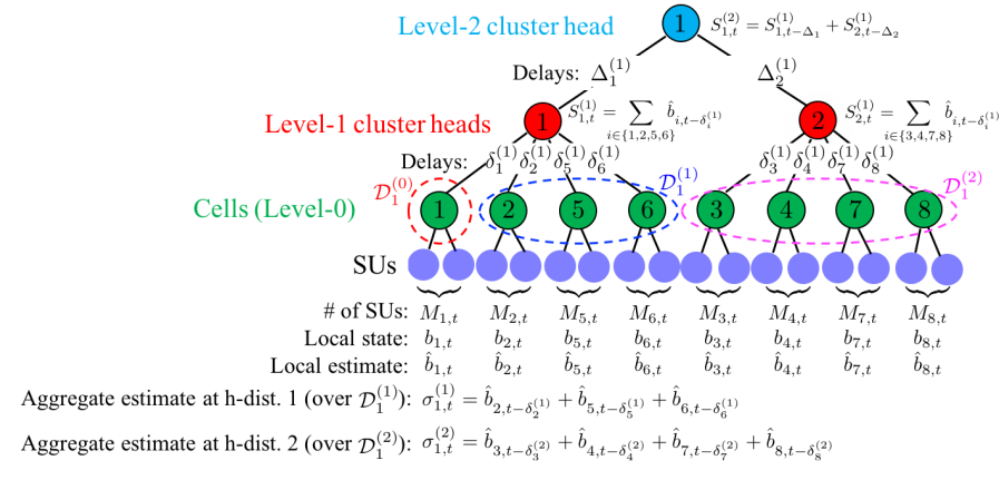
Figure 2: Aggregation process referred to Fig. 1, and aggregate estimates relative to cell $1$.

We assume that $\delta_{i}^{(L)}{\leq}\delta_{i}^{(L+1)}$, i.e., the delay augments as the local spectrum estimates are aggregated at higher levels. More precisely, let $\Delta_{m}^{(L-1)}$ be the delay between the level-$(L{-}1)$ cluster head $m$, and its level-$L$ cluster head $n$, with $m\in\mathcal{H}_{n}^{(L-1)}$. We can thus express $\delta_{i}^{(L)}$ as

$$\delta_{i}^{(L)}=\delta_{i}^{(L-1)}+\Delta_{h_{i}}^{(L-1)}=\sum_{l=1}^{L}\Delta_{h_{i}}^{(l-1)},$$ (20)

where $h_{i}^{(l)}$ is the level-$l$ cluster head of cell $i$. By the end of the spectrum sensing phase, the level-$1$ cluster head $m{\in}\mathcal{H}^{(1)}$ receives the spectrum estimates from its cluster $\mathcal{C}_{m}^{(1)}$: $\hat{b}_{i,t-\delta_{i}^{(1)}}$ is received from cell $i{\in}\mathcal{C}_{m}^{(1)}$ with delay $\delta_{i}^{(1)}{\geq}0$. These are aggregated at the level-$1$ cluster head as

$$S_{m,t}^{(1)}\triangleq\sum_{i\in\mathcal{C}_{m}^{(1)}}\hat{b}_{i,t-\delta_{i}^{(1)}},\ \forall m\in\mathcal{H}^{(1)},$$ (21)

each with its own delay. This process continues up the hierarchy: the level-$L$ cluster head $m{\in}\mathcal{H}^{(L)}$ receives $S_{k,t-\delta}^{(L-1)}$ from the level-$(L{-}1)$ cluster heads $k{\in}\mathcal{H}_{m}^{(L-1)}$ connected to it, with delay $\Delta_{k}^{(L-1)}$, and aggregates them as

$$S_{m,t}^{(L)}=\sum_{k\in\mathcal{H}_{m}^{(L-1)}}S_{k,t-\Delta_{k}}^{(L-1)},$$ (22)

each with its own delay $\Delta_{k}^{(L-1)}$. Importantly, these delays may differ from each other, hence $S_{m,t}^{(L)}$ does not truly reflect the aggregate spectrum at a given time. For this reason we denote $S_{m,t}^{(L)}$ as the delay mismatched aggregate spectrum estimate at level-$L$ cluster head $m$. The next lemma relates $S_{m,t}^{(L)}$ to the local estimates.

Lemma 1.

Let $m\in\mathcal{H}^{(L)}$ be a level-$L$ cluster head. Then,

$$S_{m,t}^{(L)}=\sum_{j\in\mathcal{C}_{m}^{(L)}}\hat{b}_{j,t-\delta_{j}^{(L)}}.$$ (23)

Proof.

See Appendix A. ∎

Despite mismatched delays, in Sec. IV we show that cell $i$ can compensate them via prediction.

Remark 2.

Note that the aggregation process runs in a decentralized fashion at each node: level-$L$ cluster head $m$ needs only information about the set of level-$(L{-}1)$ cluster heads connected to it, $k{\in}\mathcal{H}_{m}^{(L{-}1)}$, and the delays $\Delta_{k}^{(L{-}1)}$. This information is available at each node during tree formation; delays may be estimated using time-stamps associated with the control packets. The aggregation process has low complexity: each cluster-head simply aggregates the delay mismatched aggregate spectrum estimates from the lower level cluster heads connected to it, and transmits this aggregate estimate to its higher level cluster head.

Eventually, the aggregate spectrum measurements are fused at the root (level-$D$) as

$$S_{1,t}^{(D)}=\sum_{k\in\mathcal{H}_{1}^{(D-1)}}S_{k,t-\Delta_{k}}^{(D-1)}=\sum_{j\in\mathcal{C}}\hat{b}_{j,t-\delta_{j}^{(D)}},$$ (24)

where we used Lemma 1 and $\mathcal{C}_{1}^{(D)}{\equiv}\mathcal{C}$. Upon reaching level-$D$ and each of the lower levels, the aggregate spectrum estimates are propagated down to the individual cells $i{\in}\mathcal{C}$ over the tree.

Therefore, at the beginning of frame $t$, the SUs in cell $i$ receive the delay mismatched aggregate spectrum estimates from their level-$L$ cluster heads $h_{i}^{(L)},L=0,\dots,D$,

$$\left\{\begin{array}[]{rcl}S_{i,t}^{(0)}&=&\hat{b}_{i,t},\\ S_{h_{i},t}^{(L)}&=&\sum_{j\in\mathcal{C}_{h_{i}}^{(L)}}\hat{b}_{j,t-\delta_{j}^{(L)}},\ 1\leq L<D,\end{array}\right.$$

where we remind that $\mathcal{C}_{h_{i}}^{(L)}$ is the set of cells associated to $h_{i}^{(L)}$ at level $L$, and $\delta_{j}^{(L)}$ is the delay for the estimate of $b_{j,t}$ to propagate to the level-$L$ cluster head $h_{i}^{(L)}$. From this set of measurements, cell $i$ can compute the aggregate spectrum estimate of the cells at all h-distances from itself as

$$\left\{\begin{array}[]{lcl}\sigma_{i,t}^{(0)}&\triangleq&S_{h_{i},t}^{(0)}=\hat{b}_{i,t},\\ \sigma_{i,t}^{(L)}&\triangleq&S_{h_{i},t}^{(L)}{-}S_{h_{i},t-\Delta_{h_{i}}}^{(L-1)},\ 1{\leq}L{\leq}D.\end{array}\right.$$ (27)

To interpret $\sigma_{i,t}^{(L)}$ as the aggregate estimate at h-distance $L$ from cell $i$, note that Lemma 1 yields

$\sigma_{i,t}^{(L)}=\sum_{j\in\mathcal{C}_{h_{i}}^{(L)}}\hat{b}_{j,t-\delta_{j}^{(L)}}-\sum_{j\in\mathcal{C}_{h_{i}}^{(L-1)}}\hat{b}_{j,t-\delta_{j}^{(L-1)}-\Delta_{h_{i}}^{(L-1)}}.$

Since $i,j{\in}\mathcal{C}_{h_{i}}^{(L-1)}$ share the same level-$(L{-}1)$ and -$L$ cluster heads, $h_{i}^{(L-1)}$ and $h_{i}^{(L)}$, (20) yields

$\delta_{j}^{(L-1)}+\Delta_{h_{i}}^{(L-1)}=\delta_{j}^{(L)}.$

Then, $\forall\ L=1,2,\dots,D$, using Definition 2 we obtain

$$\sigma_{i,t}^{(L)}{=}\sum_{j\in\mathcal{C}_{h_{i}}^{(L)}}\hat{b}_{j,t-\delta_{j}^{(L)}}-\sum_{j\in\mathcal{C}_{h_{i}}^{(L-1)}}\hat{b}_{j,t-\delta_{j}^{(L)}}{=}\sum_{j\in\mathcal{D}_{i}^{(L)}}\hat{b}_{j,t-\delta_{j}^{(L)}},$$ (28)

so that $\sigma_{i,t}^{(L)}$ represents the delay mismatched aggregate spectrum estimate of cells at h-distance $L$ from cell $i$ ($j{\in}\mathcal{D}_{i}^{(L)}$). Thus, with this method, the SUs in cell $i$ can compute the delay mismatched aggregate estimate at multiple scales corresponding to different h-distances, given delayed measurements. Notably, only aggregate and delayed estimates are available, rather than timely information on the state of each cell. These are used to update the belief $\pi_{i,t}$ in Sec. IV.

IV Analysis

Given past and current delayed spectrum estimates across all h-distances, $\bm{\sigma}_{i,\tau}{=}(\sigma_{i,\tau}^{(0)},\sigma_{i,\tau}^{(1)},\dots,\sigma_{i,\tau}^{(D)}),$ $\tau{=}0,\dots,t$, the form of the local belief $\pi_{i,t}$ is provided in the following theorem.

Theorem 1.

Given $\bm{\sigma}_{i,\tau},\tau=0,1,\dots,t$, we have

$$\pi_{i,t}(\mathbf{b}){=}\prod_{L=0}^{D}\mathbb{P}\left(b_{j,t}{=}b_{j},\forall j\in\mathcal{D}_{i}^{(L)}|\sigma_{i,\tau}^{(L)},\forall\tau=0,\dots,t\right),$$ (29)

where, letting $x=\sum_{j\in\mathcal{D}_{i}^{(L)}}b_{j}$,

$$\mathbb{P}\Bigr{(}b_{j,t}=b_{j},\forall j\in\mathcal{D}_{i}^{(L)}\Bigr{|}\sigma_{i,\tau}^{(L)},\forall\tau=0,\dots,t\Bigr{)}\\ =\sum_{x=0}^{|\mathcal{D}_{i}^{(L)}|}\underbrace{\mathbb{P}\Bigr{(}\sum_{j\in\mathcal{D}_{i}^{(L)}}b_{j,t-\delta_{j}^{(L)}}=x\Bigr{|}\sigma_{i,\tau}^{(L)},\forall\tau=0,\dots,t\Bigr{)}}_{\text{A}}\\ \times\underbrace{\frac{x!|\mathcal{D}_{i}^{(L)}-x|!}{|\mathcal{D}_{i}^{(L)}|!}}_{\text{B}}\sum_{\tilde{b}_{j},j\in\mathcal{D}_{i}^{(L)}}\underbrace{\chi\Bigr{(}\sum_{l\in\mathcal{D}_{i}^{(L)}}\tilde{b}_{l}=x\Bigr{)}}_{\text{C}}\\ \times\prod_{l\in\mathcal{D}_{i}^{(L)}}\underbrace{\left[\pi_{B}{+}\mu^{\delta_{l}^{(L)}}\left(\tilde{b}_{l}{-}\pi_{B}\right)\right]^{b_{l}}}_{\text{D}}\underbrace{\left[1{-}\pi_{B}{-}\mu^{\delta_{l}^{(L)}}\left(\tilde{b}_{l}{-}\pi_{B}\right)\right]^{1{-}b_{l}}}_{\text{E}},$$ (30)

where $\chi(\cdot)$ is the indicator function. Additionally,

$$\mathbb{E}\Bigr{(}\sum_{j\in\mathcal{D}_{i}^{(L)}}b_{j,t-\delta_{j}^{(L)}}\Bigr{|}\sigma_{i,\tau}^{(L)},\forall\tau=0,\dots,t\Bigr{)}=\sigma_{i,t}^{(L)}.$$ (31)

Proof.

See Appendix B. ∎

We note the following facts related to Theorem 1:

1. Equation (29) implies that $\pi_{i,t}$ is statistically independent across the subsets of cells at different h-distances from cell $i$; this result follows from Assumption 1, which guarantees independence of spectrum occupancies and spectrum sensing across cells.

2. Equation (30) contains five terms. "$A$" is the probability distribution of the delay mismatched aggregate spectrum occupancy given past estimates. "$B$" is the probability of a specific realization of $b_{j,t-\delta_{j}^{(L)}},j{\in}\mathcal{D}_{i}^{(L)}$, given that its aggregate equals $x$, whereas "C" is the marginal over all these realizations; since there are $|\mathcal{D}_{i}^{(L)}|!/x!/(|\mathcal{D}_{i}^{(L)}|{-}x)!$ combinations of such spectrum occupancies, Assumption 1 implies that they are uniformly distributed, yielding "$B$". Finally, terms "$D$" and "$E$" represent the $\delta_{l}^{(L)}$ steps transition probability from $b_{l-\delta_{l}^{(L)}}{=}\tilde{b}_{l}$ to $b_{j,t}{=}1$ and $b_{j,t}{=}0$, respectively.

3. Equation (31) states that the expected delay mismatched aggregate occupancy over $\mathcal{D}_{i}^{(L)}$ equals $\sigma_{i,t}^{(L)}$, independently of past spectrum estimates. However, its probability distribution ("$A$" in (30)) does depend on past estimates.

4. In general, the term "$A$" in (30) cannot be computed in closed form, except in some special cases (e.g., noiseless measurements [2]). However, we will now show that a closed-form expression is not required to compute $I_{P,i}(\pi_{i,t})$, hence the expected utility in cell $i$ via (II). To this end, in the next lemma we compute $\mathbb{P}(b_{j,t}{=}1|\pi_{i,t})$ in closed form.

Lemma 2.

For $j\in\mathcal{D}_{i}^{(L)}$, i.e., we have

$$\mathbb{P}(b_{j,t}=1|\pi_{i,t})=\pi_{B}+\mu^{\delta_{j}^{(L)}}\Biggr{(}\frac{\sigma_{i,t}^{(L)}}{|\mathcal{D}_{i}^{(L)}|}-\pi_{B}\Biggr{)}.$$ (32)

Proof.

See Appendix C. ∎

We now compute $I_{P,i}(\pi_{i,t})$. Partitioning $\mathcal{C}$ based on the h-distances from $i$, (9) yields

$$I_{P,i}(\pi_{i,t})\triangleq\sum_{L=0}^{D}\sum_{j\in\mathcal{D}_{i}^{(L)}}\frac{\phi_{j,i}}{\phi_{i,i}}\mathbb{P}\left(b_{j,t}=1|\pi_{i,t}\right).$$ (33)

Then, substituting (32) in (33) and letting

$$\left\{\begin{array}[]{l}\Phi_{\mathrm{tot},i}\triangleq\sum_{j\in\mathcal{C}}\frac{\phi_{j,i}}{\phi_{i,i}},\\ \Phi_{\mathrm{del},i}^{(L)}\triangleq\sum_{j\in\mathcal{D}_{i}^{(L)}}\mu^{\delta_{j}^{(L)}}\frac{\phi_{j,i}}{\phi_{i,i}}\end{array}\right.$$ (36)

be the total mutual interference generated between the SUs in cell $i$ and the PU network ($\Phi_{\mathrm{tot},i}$), and the delay compensated mutual interference generated between cell $i$ and the cells at h-distance $L$ from cell $i$ ($\Phi_{\mathrm{del},i}^{(L)}$), we obtain the following lemma.

Lemma 3.

The expected PU activity experienced in cell $i$ is given by

$$I_{P,i}(\bm{\sigma}_{i,t})\triangleq\pi_{B}\Phi_{\mathrm{tot},i}+\sum_{L=0}^{D}\Biggr{(}\frac{\sigma_{i,t}^{(L)}}{|\mathcal{D}_{i}^{(L)}|}-\pi_{B}\Biggr{)}\Phi_{\mathrm{del},i}^{(L)}.$$ (37)

Above, for convenience, we have expressed the dependence of $I_{P,i}(\cdot)$ on $\bm{\sigma}_{i,t}$, rather than on $\pi_{i,t}$. Thus, the local utility (II) can be computed accordingly. Note that $I_{P,i}(\bm{\sigma}_{i,t})$ depends on the clustering of cells across multiple spatial scales that affect the delay mismatched aggregate spectrum estimates $\sigma_{i,t}^{(L)}$, hence on the tree employed for hierarchical information exchange. In the next section, we propose a tree design matched to the structure of interference.

V Tree Design

The network utility depends crucially on the tree employed for information exchange. Its optimization over all possible trees is a combinatorial problem with high complexity. Thus, we use agglomerative clustering, developed in [16, Ch. 14], in which a tree is built by successively combining smaller clusters based on a "closeness" metric, that we now develop.

Note that in our problem the goal is for cell $i$ to estimate the INR generated to the PUs as accurately as possible, $\sum_{j=1}^{N_{C}}\frac{\phi_{j,i}}{\phi_{i,i}}b_{j,t}$. This estimate is denoted as $I_{P,i}(\pi_{i,t})$, see (9). In fact, given $I_{P,i}(\pi_{i,t})$, SUs in cell $i$ can schedule the optimal SU traffic $a_{i,t}^{*}(I_{P,i}(\pi_{i,t}))$ via (II), hence the optimal utility via (II). With the hierarchical information exchange described in the previous section, this estimate is given by (37).

Therefore, the goal is to design the tree in such a way as to estimate $\sum_{j=1}^{N_{C}}\frac{\phi_{j,i}}{\phi_{i,i}}b_{j,t}$ as accurately as possible via $I_{P,i}(\bm{\sigma}_{i,t})$ in (37). At the same time, since all cells share the same tree, such design should take into account this goal across all cells. We develop a heuristic metric to attain this goal. To this end, we notice the following facts: 1) since higher levels correspond to larger and larger clusters over which spectrum estimates are aggregated (for instance, with reference to Fig. 1, $|\mathcal{D}_{1}^{(0)}|{=}1$, $|\mathcal{D}_{1}^{(1)}|{=}3$ and $|\mathcal{D}_{1}^{(2)}|{=}4$ at h-distances $0,1,2$, respectively), higher levels correspond to coarser estimates of spectrum occupancy, whereas lower levels correspond to fine-grained estimates; 2) from (37), it is apparent that terms with larger $\Phi_{\mathrm{del},i}^{(L)}$ affect more strongly $I_{P,i}(\bm{\sigma}_{i,t})$. Therefore, cluster aggregation resulting in larger $\Phi_{\mathrm{del},i}^{(L)}$ should occur at lower hierarchical levels, associated with fine-grained estimation. Taking these facts into account, we denote the "aggregation" metric between $n,m{\in}\mathcal{H}^{(L)}$ as

$$\Gamma_{n,m}^{(L)}{=}\mu^{\Delta_{n,m}}\Biggr{[}\sum_{i\in\mathcal{C}_{n}^{(L)}}\sum_{j\in\mathcal{C}_{m}^{(L)}}\mu^{\delta_{j}^{(L)}}\frac{\phi_{j,i}}{\phi_{i,i}}{+}\sum_{i\in\mathcal{C}_{m}^{(L)}}\sum_{j\in\mathcal{C}_{n}^{(L)}}\mu^{\delta_{j}^{(L)}}\frac{\phi_{j,i}}{\phi_{i,i}}\Biggr{]}.$$ (38)

$\Gamma_{n,m}^{(L)}$ represents the benefit of aggregating together the clusters associated to level-$L$ cluster-heads $m$ and $n$, $\mathcal{C}_{m}^{(L)}$ and $\mathcal{C}_{n}^{(L)}$, respectively, into one level-$(L{+}1)$ cluster, and $\Delta_{n,m}$ is the additional delay incurred to aggregate them. In fact, if such aggregation occurs, from the perspective of cell $i\in\mathcal{C}_{n}^{(L)}$, $\mathcal{C}_{m}^{(L)}$ will become the set of cells at h-distance $L+1$ from cell $i$, $\mathcal{D}_{i}^{(L+1)}\equiv\mathcal{C}_{m}^{(L)}$, so that, letting $\delta_{j}^{(L+1)}{=}\Delta_{n,m}{+}\delta_{j}^{(L)}$ as in (20), the first term associated to $i$ in (38) is equivalent to

$$\sum_{j\in\mathcal{C}_{m}^{(L)}}\mu^{\Delta_{n,m}+\delta_{j}^{(L)}}\frac{\phi_{j,i}}{\phi_{i,i}}=\Phi_{\mathrm{del},i}^{(L+1)}.$$ (39)

The second term in (38) has a similar interpretation, relative to cell $i\in\mathcal{C}_{m}^{(L)}$. Thus, the aggregation metric $\Gamma_{n,m}^{(L)}$ corresponds to $\sum_{i\in\mathcal{C}_{n}^{(L)}}\Phi_{\mathrm{del},i}^{(L+1)}+\sum_{i\in\mathcal{C}_{m}^{(L)}}\Phi_{\mathrm{del},i}^{(L+1)}$, if clusters $\mathcal{C}_{n}^{(L)}$ and $\mathcal{C}_{m}^{(L)}$ are aggregated together. As justified previously, this quantity should be made as large as possible in order to maximize the informativeness of the aggregation of estimates.

In addition, we want to limit the cost incurred to send measurements up and down the hierarchy. Assuming that estimates are transmitted via multi-hop, the cost will be proportional to the distance between clusters. Thus, each time we combine two clusters $\mathcal{C}_{n}^{(L)}$ and $\mathcal{C}_{m}^{(L)}$ to form the tree, we incur an additional aggregation cost per cell $C_{n,m}$, defined as

$$C_{n,m}\ =\frac{1}{N_{C}}\max_{i\in\mathcal{C}_{n}^{(L)},j\in\mathcal{C}_{m}^{(L)}}d_{i,j},$$ (40)

representing the worst-case aggregation cost, where $d_{i,j}$ is the distance between cells $i$ and $j$.

input : Cells $\mathcal{C}$, interference matrix $\bm{\Phi}$, max cost $C_{\max}$ (per cell)

output : A hierarchy of clusters $\mathcal{C}_{k}^{(L)}$, $k\in\mathcal{H}^{(L)}$, $L=1,\dots,D$, delays $\delta_{i}^{(L)}$, and aggregation cost $C_{\mathrm{cell}}$

Initialize: $L{\leftarrow}0$, $\mathcal{H}^{(L)}{\leftarrow}\mathcal{C}$, $\mathcal{C}_{i}^{(0)}{\leftarrow}\{i\}$, $\delta_{i}^{(0)}{=}0,\forall i{\in}\mathcal{C}$, $C_{\mathrm{cell}}{=}0$;

repeat

       $\Delta_{n,m},C_{n,m},\forall n,m\in\mathcal{H}^{(L)},n\neq m$ (delays and cost are computed, e.g., $\propto$#hops);

       $\mathcal{F}^{(L)}{\leftarrow}\{(n,m){\in}\mathcal{H}^{(L)2}:n,{\neq}m,C_{\mathrm{cell}}{+}C_{n,m}{\leq}C_{\max}\}$ (set of unpaired feasible pairs);

       if  $|\mathcal{F}^{(L)}|=0$ (cost exceeded)  then

             terminate

      $\mathcal{H}^{(L+1)}\leftarrow\emptyset$, $k_{next}\leftarrow 1$ (empty set of next level cluster heads and cluster head counter);

       $\mathcal{H}^{(L)}_{unp}\leftarrow\mathcal{H}^{(L)}$ (set of unpaired cluster heads);

       while $|\mathcal{F}^{(L)}|>0$ do

             $(n^{*},m^{*}){\leftarrow}\underset{(n,m){\in}\mathcal{F}^{(L)}}{\arg\max}\Gamma_{n,m}^{(L)}$ (find unpaired feasible cluster pair with max $\Gamma$, see (38));

             $\mathcal{H}^{(L+1)}\leftarrow\mathcal{H}^{(L+1)}\cup\{k_{next}\},\ \mathcal{C}_{k_{next}}^{(L+1)}\leftarrow\mathcal{C}_{n^{*}}^{(L)}\cup\mathcal{C}_{m^{*}}^{(L)}$;

             $\delta_{i}^{(L+1)}{=}\delta_{i}^{(L)}{+}\Delta_{n^{*},m^{*}},\forall i{\in}\mathcal{C}_{k_{next}}^{(L+1)},C_{\mathrm{cell}}{\leftarrow}C_{\mathrm{cell}}{+}C_{n^{*},m^{*}}$ (update delay and cost);

             $\mathcal{H}_{unp}^{(L)}\leftarrow\mathcal{H}_{unp}^{(L)}\setminus\{n^{*},m^{*}\}$ (remove paired clusters);

             $\mathcal{F}^{(L)}\leftarrow\{(n,m){\in}\mathcal{H}_{unp}^{(L)}\times\mathcal{H}_{unp}^{(L)}:n,{\neq}m,C_{\mathrm{cell}}{+}C_{n,m}{\leq}C_{\max}\}$ (updated feasible pairs);

             $k_{next}\leftarrow k_{next}+1$ ;

            

      forall $k\in\mathcal{H}_{unp}^{(L)}$ (unpaired clusters incur excessive cost, “pair” each with itself) do

             $\mathcal{H}^{(L+1)}\leftarrow\mathcal{H}^{(L+1)}\cup\{k_{next}\},\ \mathcal{C}_{k_{next}}^{(L+1)}\leftarrow\mathcal{C}_{k}^{(L)}$ ;

             $\delta_{i}^{(L+1)}=\delta_{i}^{(L)},\forall i\in\mathcal{C}_{k_{next}}^{(L+1)}$ (no additional delay/cost);

             $k_{next}\leftarrow k_{next}+1$ ;

            

      $L\leftarrow L+1$ (Proceed to the next level);

      

until termination;

Algorithm 1 Hierarchical Aggregation Tree Construction

The algorithm proceeds as shown in Algorithm 1. We initialize it with the $N_{C}$ sets containing the single cells, $\mathcal{C}_{i}^{(0)}=\{i\},i=1,2,\dots,N_{C}$, and aggregation cost (per cell) $C_{\mathrm{cell}}=0$. Then, at each level-$L$, we iterate over all cluster pairs, pairing those with highest aggregation metric $\Gamma$. This forms the set of level-$(L+1)$ clusters; we update the delays accordingly and update $C_{\mathrm{cell}}$ by adding $C_{n^{*},m^{*}}^{(L)}$. If the number of clusters at level-$L$ happens to be odd, one cluster may not be paired, in which case it forms its own level-$(L{+}1)$ cluster, and the delay remains unchanged. The algorithm proceeds until either: (1) the cluster $\mathcal{C}_{1}^{(L)}$ contains the entire network, i.e., a tree has been formed, or (2) $C_{\mathrm{cell}}>C_{\mathrm{max}}$, i.e., the allowed cost is exceeded. Agglomerative clustering has complexity $O(N_{C}^{2}\log(N_{C}))$, where the term $N_{C}^{2}$ owes to searching over all pairs of clusters, and the term $\log(N_{C})$ is related to the tree depth, which is logarithmic in the number of cells [16, Ch. 14]. In the next section, we will compare our scheme with the consensus-based scheme [17]: this scheme requires a "connected" graph to achieve consensus, whose complexity is $O(N_{C}^{3}d)$, with $d$ being the desired degree of each node in the graph [27]. Therefore, by leveraging the tree structure, our tree construction is more computationally efficient. However, tree design will be executed only at initialization, or when the network topology changes, which is infrequent in fixed cellular networks as considered in this work, hence it is not expected to have a significant impact on the long-term performance.

VI Numerical Results

In this section, we provide numerical results based on Monte Carlo simulations. We adopt a model with stochastic blockage [28]: rectangular blockages of fixed height and width are placed randomly on the boundaries between cells. Each blockage has width $1$ and height $5$, and is randomly placed. We say that links between cells $i,j$ are line of sight (LOS) if the line segment connecting the centers of cells $i$ and $j$ does not intersect any blockage object. Otherwise, such links are said to be non-LOS (NLOS). Accordingly, we define LOS and NLOS large-scale pathloss exponents $\alpha_{L}{=}2.1$ and $\alpha_{N}{=}3.3$, respectively. These values were derived experimentally in [24, Table I] at a reference frequency of $2\mathrm{GHz}$.

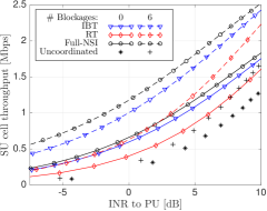
(a) Impact of blockages, delay parameter $\gamma=0$.

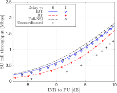
(b) Impact of delay, $1$ blockage.

Figure 3: SU cell throughput versus average INR experienced at PUs, cost constraint $C_{\max}=\infty$.

In the simulations, we consider a $16{\times}16$ cells network over an area of $1.6\mathrm{\mathrm{k}m}{\times}1.6\mathrm{\mathrm{k}m}$. We set the parameters as follows: SINR decoding threshold $\mathrm{SINR}_{\mathrm{th}}{=}5\mathrm{dB}$, noise power spectral density $N_{0}{=}-173\mathrm{dBm/Hz}$, bandwidth $W_{tot}{=}20\mathrm{MHz}$, $\nu_{1}{=}0.005$, $\nu_{0}{=}0.095$, hence $\pi_{B}{=}0.05$ and $\mu{=}0.9$. The interference matrix $\bm{\Phi}$ is calculated as in (II), where $P_{tx}{=}{-}11\mathrm{dBm}$ is the transmission power, common to all PUs and SUs, $L_{ref}{=}74\mathrm{dB}$ is the large-scale pathloss based on Friis’ free space propagation, calculated at a reference distance $d_{ref}{=}50\mathrm{m}$ (equal to the average cell radius); $\alpha_{i,j}{=}\alpha_{L}$ if there is LOS between the centers of cells $i$ and $j$, otherwise, $\alpha_{i,j}{=}\alpha_{N}$ in case of NLOS (path obstructed by blockage).

We assume that local estimation is error-free ($\epsilon_{F}{=}\epsilon_{M}{=}0$) and $M_{i,t}{\gg}1,\forall i,t$, corresponding to a dense setup with large number of SUs. In this work, we do not consider the overhead of local spectrum sensing within each cell, which can be severe in dense networks and may be reduced by using decentralized techniques to select the most informative SUs, such as in [8]; these considerations are outside the scope of this paper, and are left for future work. We average the results over $200$ realizations of the blockage model. For each one of these, we generate a sequence of $1000$ frames to generate the Markov process $\{\mathbf{b}_{t},t\geq 0\}$. We consider the following schemes:

• a scheme with the interference-based tree (IBT) generated with Algorithm 1 by leveraging the specific structure of interference, delays and aggregation costs;

• a scheme with a random tree (RT), in which the "max $\Gamma$" cluster association in Algorithm 1 is replaced with a random association. The aim of using this scheme is to test the importance of generating a tree matched to the structure interference;

• a scheme with full (but delayed) NSI (Full-NSI); since this scheme represents the best we can do, provided that we can afford the cost of acquisition of full NSI, it will be used to evaluate the sub-optimality of the proposed IBT in terms of the trade-off between SU cell throughput and interference to PUs;

• an uncoordinated scheme where SUs access the spectrum with constant probability $p_{tx}$, i.i.d. over time and across SUs (Uncoordinated).

We assume that the delay to propagate spectrum measurements between cells $i$ and $j$ is proportional to their distance, i.e., $\delta_{i,j}=\gamma d_{i,j}$, where $\gamma$ is varied in $[0,1]$.

In order to separate the effects of blockages, delay, and cost of aggregation on the performance, we evaluate the impact of: 1) Blockages, but no delay nor cost constraint ($\gamma{=}0$, $C_{\max}{=}\infty$, Fig. 3(a)); 2) Delay, with one blockage but no cost constraint (1 blockage, $C_{\max}{=}\infty$, Fig. 3(b)); 3) Cost of aggregation, with one blockage and no delay (1 blockages, $\gamma{=}0$, Fig. 4). In all these figures, unless otherwise stated, we evaluate the lower bound to the SU cell throughput, given by (II) and the INR experienced at the PUs (both averaged over cells and over time). We vary the parameter $\lambda$ in the utility function (II) and the SU access probability $p_{tx}$ in the "Uncoordinated" scheme, to obtain the desired trade-off between SU cell throughput and INR.

In Fig. 3(a), we notice that, for all schemes, the presence of blockages improves the performance. In fact, blockages provide a form of interference mitigation. By comparing the schemes with each other, the best performance is obtained with Full-NSI. In fact, each cell can leverage the most refined information on the interference pattern. However, as we will see in Fig. 4, this comes at a huge cost to propagate NSI over the network. Remarkably, IBT incurs only a 15% (for 6 blockages) and 10% (for no blockages) performance degradation with respect to Full-NSI, for a reference INR of $0$dB (this result becomes more remarkable when comparing the aggregation costs in Fig. 4). Additionally, RT incurs a severe performance degradation with respect to IBT (60% and 30% degradation for 6 blockages and no blockages, respectively, for a reference INR of $0$dB); this fact highlights the importance of designing a tree matched to the structure of interference, as done in Algorithm 1, and validates our choice of the $\Gamma$ metric used to associate clusters in the algorithm, defined in (38). Finally, we observe that the "Uncoordinated" scheme performs the worst, since it does not adapt the SU transmissions to interference.

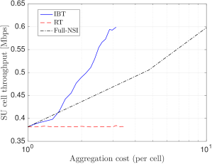
Figure 4: Impact of aggregation cost on the SU cell throughput, with $0$dB maximum constraint on the average INR caused to PUs. $1$ blockage; no delay.

In Fig. 3(b), we evaluate the impact of delay (note that "Uncoordinated" is not affected by delays). As expected, the SU cell throughput decreases as the delay augments. This follows from the fact that delayed spectrum estimates represent less accurately the actual spectrum occupancy, and may become outdated, and thus less informative for scheduling decisions of SUs. However, the performance degradation is minimal. In fact, the spectrum occupancy varies slowly over time: the expected duration of a period during which the spectrum is occupied by a PU is $1/\nu_{0}{\simeq}10$ frames, hence only the spectrum estimates received with delay larger than 10 become non informative; these estimates, in turn, correspond to cells that are farther away from the reference cell, hence less susceptible to interference caused by the reference cell. We notice a similar trend as in Fig. 3(a) in terms of the comparison among the schemes employed.

In Fig. 4, we evaluate the trade-off between aggregation cost and performance. To this end:

• We vary the cost constraint $C_{\max}$ in Algorithm 1 to obtain a trade-off for IBT and RT; we use a "worst-case" cost evaluation with multi-hop, given by (40).

• To evaluate Full-NSI, each cell collects partial but fine-grained NSI up to a certain radius; larger radius corresponds to more comprehensive NSI but larger cost; using multi-hop for NSI aggregation, the cost equals approximately the number of cells within the radius. This scheme borrows from [13], where each cell informs neighboring ones of the resource blocks used by its users.

We notice that IBT achieves a much better trade-off than Full-NSI: it enables SUs to gather relevant information for scheduling decisions, with minimal cost in the exchange of state information. In fact, by aggregating NSI at multiple layers, as opposed to maintaining fine-grained NSI, IBT retains the gains of partial NSI, but at a much smaller cost of aggregation. In particular, for a reference SU cell throughput of 0.6Mbps, IBT incurs one-third of the cost of aggregation of Full-CSI. On the other hand, RT does not improve as the cost increases; in fact, the random tree construction in RT results in information exchange which is not matched to the structure of interference, hence less informative to network control.

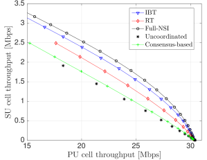
Figure 5: Simulation with random topology and realistic large-scale pathloss. Comparison with "consensus" scheme [17].

So far, in our analysis and numerical evaluation we have assumed that large-scale pathloss is calculated between cell centers, and collected in the INR matrix $\bm{\Phi}$. However, large-scale pathloss between a transmitter and a receiver depends on their mutual position within their respective cell. Additionally, we used the SU cell throughput lower bound (II). This motivates us to evaluate the performance in a more realistic scenario, where these assumptions are relaxed. In Fig. 5, we evaluate a realistic scenario with the following features:

• We generate $100$ independent realizations of the network topology with $N_{C}{=}256$ PU cells; in each realization, the transmitter-receiver pairs are deployed randomly over an area of $1.6\mathrm{\mathrm{k}m}{\times}1.6\mathrm{\mathrm{k}m}$; an irregular cell topology is thus defined based on minimum distance; 10 SUs are deployed randomly in each cell (each with its own receiver).

• The large-scale pathloss is computed between each transmitter and receiver based on their relative distance, as in (II). The INR matrix $\bm{\Phi}$ is computed relative to the cell centers. This is used to construct the hierarchical aggregation tree (Algorithm 1), to estimate $I_{S,i}(t)$ and $I_{P,i}(\pi_{i,t})$ as in (8) and (9), hence to compute the optimal SU traffic $a_{i,t}^{*}$ as in (II). However, the performance is evaluated under the actual distance-dependent large-scale pathloss and the realization of the Rayleigh fading process, as described in the next item.

• For each realization of the network topology, we generate 1000 frames with random SU access decisions; the PU spectrum occupancy process $\mathbf{b}_{t}$ evolves according to the Markov process described in Sec. II, with $\nu_{1}{=}0.005$, $\nu_{0}{=}0.095$; in each frame, the channel is generated according to the distance-dependent large-scale pathloss and Rayleigh fading distribution, independent over time and across users, as described in the signal model (2). The SINR is then computed at each SU and PU receiver, and the transmission is declared successful if and only if SINR${>}\mathrm{SINR}_{\mathrm{th}}{=}5\mathrm{dB}$. The SU and PU cell throughputs are then averaged out over the 1000 frames and 100 realizations of the network topology.

In addition to IBT, RT, Full-CSI and Uncoordinated schemes mentioned previously, we also evaluate the performance of the consensus-based scheme [17]. We set the degree of each node (cell head) to be $d=5$, based on which we generate a connected graph [27]. This scheme was originally designed for a single PU cell system without temporal dynamics in the PU spectrum occupancy, and therefore it is not optimized to our model, with multiple cells and temporal dynamics of spectrum occupancy in each cell. We argue that a consensus-based scheme, such as [17], is not well suited to capture the spatial distribution of interference, nor the temporal dynamics, due to the averaging process of consensus in both the spatial and temporal dimensions. Instead, our scheme allows each SU to estimate accurately the state of nearer cells, to which interference will be stronger, and to track more efficiently their temporal dynamics. Our numerical evaluation in Fig. 5 confirms this observation: the consensus strategy performs poorly, with performance close to the "Uncoordinated" scheme. On the other hand, the performance of IBT is very close to that of Full-NSI and significantly outperforms the "Uncoordinated" scheme. This evaluation confirms that, despite the approximation introduced in the INR matrix $\bm{\Phi}{\in}\mathbb{R}^{N_{C}\times N_{C}}$, our multi-scale spectrum estimation positively informs network control.

VII Conclusions

In this paper, we have proposed a multi-scale approach to spectrum sensing in cognitive cellular networks. To reduce the cost of acquisition of NSI, we have proposed a hierarchical scheme to obtain aggregate state information at multiple scales, at each cell. We have studied analytically the performance of the aggregation scheme in terms of the trade-off among the SU cell throughput, the interference generated by their activity to PUs, and the mutual interference of SUs. We have accounted for aggregation delays, local estimation errors, as well as the cost of aggregation. We have proposed an agglomerative clustering algorithm to find a multi-scale aggregation tree, matched to the structure of interference. We have shown that our proposed design achieves performance close to that with full NSI, using only one-third of the cost of exchange of spectrum estimates over the network.

Appendix A: Proof of Lemma 1

Proof.

We prove it by induction. At level-$1$, (23) holds by definition, see (21). Now, let $L{>}1$ and assume (23) holds at level-$(L{-}1)$. The induction hypothesis in (22) implies

$$S_{m,t}^{(L)}=\sum_{k\in\mathcal{H}_{m}^{(L-1)}}\sum_{j\in\mathcal{C}_{k}^{(L-1)}}\hat{b}_{j,t-\delta_{j}^{(L-1)}-\Delta_{k}^{(L)}}.$$ (41)

Then, using (20) we obtain

$$S_{m,t}^{(L)}=\sum_{k\in\mathcal{H}_{m}^{(L-1)}}\sum_{j\in\mathcal{C}_{k}^{(L-1)}}\hat{b}_{j,t-\delta_{j}^{(L)}}=\sum_{j\in\mathcal{C}_{m}^{(L)}}\hat{b}_{j,t-\delta_{j}^{(L)}},$$ (42)

where the last step follows from (16). The induction step, hence the lemma, are thus proved. ∎

Appendix B: Proof of Theorem 1

Proof.

Let $t\geq 0$. Eq. (29) follows from the fact that $\sigma_{i,t}^{(L)}$ is independent of $b_{j,\tau},\forall\tau\leq t$ for $j\notin\mathcal{D}_{i}^{(L)}$, and from the fact that $(b_{j,\tau},M_{j,\tau},\xi_{j,\tau}),\tau\leq t$ are independent across cells.

We now prove (30) for a given set $\mathcal{D}_{i}^{(L)}$ and h-distance $L$. With a slight abuse of notation, "$\forall j$" should be intended as "$\forall j{\in}\mathcal{D}_{i}^{(L)}$", and "$\sum_{j}$" as "$\sum_{j\in\mathcal{D}_{i}^{(L)}}$". Using (28),

$$\mathbb{P}\Bigr{(}b_{j,t}=b_{j},\forall j\Bigr{|}\sigma_{i,\tau}^{(L)}=o_{\tau}^{(L)},\forall\tau\leq t\Bigr{)}$$

$$=\mathbb{P}\Bigr{(}b_{j,t}=b_{j},\forall j\Bigr{|}\sum_{j}\hat{b}_{j,\tau-\delta_{j}^{(L)}}=o_{\tau}^{(L)},\forall\tau\leq t\Bigr{)}.$$

We can rewrite it as the marginal with respect to $b_{j,t-\delta_{j}^{(L)}},\forall j$ and $\sum_{j}b_{j,t-\delta_{j}^{(L)}}=x$, yielding

$$\mathbb{P}\left(b_{j,t}=b_{j},\forall j\left|\sigma_{i,\tau}^{(L)}=o_{\tau}^{(L)},\forall\tau\leq t\right.\right)$$ (43)

$$=\sum_{x=0}^{|\mathcal{D}_{i}^{(L)}|}\sum_{(\tilde{b}_{j,t-\delta_{j}^{(L)}})_{\forall j}}\mathbb{P}\Bigr{(}b_{j,t}=b_{j},\forall j\Bigr{|}b_{j,t-\delta_{j}^{(L)}}{=}\tilde{b}_{j,t-\delta_{j}^{(L)}},\forall j,$$

$$\quad\quad\sum_{j}b_{j,t-\delta_{j}^{(L)}}{=}x,\sum_{j}\hat{b}_{j,\tau-\delta_{j}^{(L)}}=o_{\tau}^{(L)},\forall\tau\leq t\Bigr{)}$$ (D;E)

$$\times\mathbb{P}\Bigr{(}b_{j,t-\delta_{j}^{(L)}}=\tilde{b}_{j,t-\delta_{j}^{(L)}},\forall j\Bigr{|}\sum_{j}b_{j,t-\delta_{j}^{(L)}}=x,$$

$$\qquad\quad\sum_{j}\hat{b}_{j,\tau-\delta_{j}^{(L)}}=o_{\tau}^{(L)},\forall\tau\leq t\Bigr{)}$$ (B;C)

$${\times}\mathbb{P}\Bigr{(}\sum_{j}b_{j,t-\delta_{j}^{(L)}}{=}x\Bigr{|}\sum_{j}\hat{b}_{j,\tau-\delta_{j}^{(L)}}{=}o_{\tau}^{(L)},\forall\tau{\leq}t\Bigr{)}.$$ (A)

Using the fact that $\{b_{j,t}\}$ is Markov and i.i.d. across cells, for the term (D;E) we obtain

$$\mathbb{P}\Bigr{(}b_{j,t}{=}b_{j},\forall j\Bigr{|}b_{j,t-\delta_{j}^{(L)}}{=}\tilde{b}_{j,t-\delta_{j}^{(L)}},\forall j,$$

$$\qquad\sum_{j}b_{j,t-\delta_{j}^{(L)}}=x,\sum_{j}\hat{b}_{j,\tau-\delta_{j}^{(L)}}=o_{\tau}^{(L)},\forall\tau\leq t\Bigr{)}$$

$$=\prod_{j}\mathbb{P}\left(b_{j,t}=b_{j}\left|b_{j,t-\delta_{j}^{(L)}}=\tilde{b}_{j,t-\delta_{j}^{(L)}}\right.\right),$$ (44)

since $b_{j,t}$ is independent of all other quantities given $b_{j,t-\delta_{j}^{(L)}}$. In particular, the probability term in (44) is the $\delta_{j}^{(L)}$ steps transition probability of the Markov chain $\{b_{j,\tau},\forall\tau\}$, i.e.,

$$\mathbb{P}\left(b_{j,t}=b_{j}\left|b_{j,t-\delta_{j}^{(L)}}=\tilde{b}_{j}\right.\right)$$ (45)

$${=}\left[\pi_{B}{+}\mu^{\delta_{j}^{(L)}}\left(\tilde{b}_{j}{-}\pi_{B}\right)\right]^{b_{j}}\left[1{-}\pi_{B}{-}\mu^{\delta_{j}^{(L)}}\left(\tilde{b}_{j}{-}\pi_{B}\right)\right]^{1{-}b_{j}}.$$

which is equivalent to the terms $D$ and $E$ in (30). Next, letting $\mathbf{b}_{t}^{(\delta)}=(b_{j,t-\delta_{j}^{(L)}})_{\forall j}$, we show that the term (B;C) is equivalent to $B$ and $C$ in (30). In fact,

$$\mathbb{P}\Bigr{(}\mathbf{b}_{t}^{(\delta)}{=}\tilde{\mathbf{b}}\Bigr{|}\sum_{j}b_{j,t}^{(\delta)}{=}x,\sum_{j}\hat{b}_{j,\tau-\delta_{j}^{(L)}}{=}o_{\tau}^{(L)},\forall\tau\leq t\Bigr{)}$$

$$=\chi\Bigr{(}\sum_{j}\tilde{b}_{j}=x\Bigr{)}\frac{x!(|\mathcal{D}_{i}^{(L)}|-x)!}{|\mathcal{D}_{i}^{(L)}|!}.$$ (46)

We obtain (30) by substituting (44)-(46) into (43).

To see (46), first note that, if $\sum_{j}\tilde{b}_{j}\neq x$, then (46) must be zero, since we are conditioning on $\sum_{j}b_{j,t}^{(\delta)}{=}x$. Thus, we focus on the case $\sum_{j}\tilde{b}_{j}=x$. Let $s_{j}=(M_{j,\tau},{\xi}_{j,\tau})_{\forall j,-\delta_{j}^{(L)}\leq\tau\leq t-\delta_{j}^{(L)}}$ and $\tilde{s}_{j}$ be a specific realization of the estimation process. From the expression of the local estimator, we note that $\hat{b}_{j,\tau}$ is a function of $(\hat{b}_{j,\tau-1},M_{j,\tau},\xi_{j,\tau})$. Then, by induction, $\hat{b}_{j,\tau}$ is a function of $(M_{j,\tau^{\prime}},\xi_{j,\tau^{\prime}})_{-\delta_{j}^{(L)}\leq\tau^{\prime}\leq\tau}$ (and thus of $s_{j}$), denoted as

$\hat{b}_{j,\tau}=g_{\tau+\delta_{j}^{(L)}}(s_{j}).$

Note that the subscript $\tau+\delta_{j}^{(L)}$ signifies that the first $\tau+\delta_{j}^{(L)}+1$ samples of $(M_{j,\tau^{\prime}},\xi_{j,\tau^{\prime}})$ are used to compute $\hat{b}_{j,\tau}$, since $-\delta_{j}^{(L)}\leq\tau^{\prime}\leq\tau$. Importantly, $\hat{b}_{j,\tau}$ depends on the cell index $j$ only through $\delta_{j}^{(L)}$ and $s_{j}$, so that

$\sum_{j}\hat{b}_{j,\tau-\delta_{j}^{(L)}}=\sum_{j}g_{\tau}(s_{j}).$

Let $\mathcal{BS}$ be the set of tuples $(\mathbf{b},\mathbf{s})$ such that

$\sum_{j}b_{j}=x,\ \sum_{j}g_{\tau}(s_{j})=o_{\tau}^{(L)},\forall 0\leq\tau\leq t.$

Using this definition, we write the left hand side of (46) as

$$\mathbb{P}\Bigr{(}\mathbf{b}_{t}^{(\delta)}{=}\tilde{\mathbf{b}}\Bigr{|}\sum_{j}b_{j}=x,\sum_{j}\hat{b}_{j,\tau-\delta_{j}^{(L)}}=o_{\tau}^{(L)},\forall\tau\leq t\Bigr{)}$$

$$=\mathbb{P}\left(\mathbf{b}_{t}^{(\delta)}=\tilde{\mathbf{b}}\left|(\mathbf{b}_{t}^{(\delta)},\mathbf{s})\in\mathcal{BS}\right.\right).$$ (47)

Consider a permutation $\mathcal{P}:\mathcal{D}_{i}^{(L)}\mapsto\mathcal{D}_{i}^{(L)}$ of the elements in the set $\mathcal{D}_{i}^{(L)}$. Thus,

$$\left\{\begin{array}[]{l}\sum_{j}g_{\tau}(s_{\mathcal{P}(j)})=\sum_{j}g_{\tau}(s_{j}),\\ \sum_{j}b_{\mathcal{P}(j)}=\sum_{j}b_{j}=x.\end{array}\right.$$ (50)

By definition of $\mathcal{BS}$, if $(\mathbf{b},\mathbf{s}){\in}\mathcal{BS}$ then, under any permutation, $(\mathbf{b}_{\mathcal{P}},\mathbf{s}_{\mathcal{P}}){\in}\mathcal{BS}$, where $\mathbf{b}_{\mathcal{P}}=(b_{\mathcal{P}(j)})_{\forall j}$ and $\mathbf{s}_{\mathcal{P}}=(s_{\mathcal{P}(j)})_{\forall j}$. We can thus partition $\mathcal{BS}$ into $|\mathcal{U}|$ sets, $\mathcal{BS}_{u},u\in\mathcal{U}$, where $\mathcal{U}$ is a set of indexes, such that $\mathcal{BS}_{u}$ contains all and only the permutations of its elements, that is

$$\left\{\begin{array}[]{l}(\mathbf{b},\mathbf{s})\in\mathcal{BS}_{u}\Leftrightarrow(\mathbf{b}_{\mathcal{P}},\mathbf{s}_{\mathcal{P}})\in\mathcal{BS}_{u},\ \forall\mathcal{P},\\ (\mathbf{b}^{(1)},\mathbf{s}^{(1)})\in\mathcal{BS}_{u},(\mathbf{b}^{(1)},\mathbf{s}^{(1)})\neq(\mathbf{b}^{(2)}_{\mathcal{P}},\mathbf{s}^{(2)}_{\mathcal{P}}),\forall\mathcal{P}\\ \qquad\qquad\Rightarrow(\mathbf{b}^{(2)}_{\mathcal{P}},\mathbf{s}^{(2)}_{\mathcal{P}})\notin\mathcal{BS}_{u},\\ \cup_{u\in\mathcal{U}}\mathcal{BS}_{u}\equiv\mathcal{BS},\ \mathcal{BS}_{u_{1}}\cap\mathcal{BS}_{u_{2}}\equiv\emptyset,\forall u_{1}\neq u_{2}.\end{array}\right.$$ (55)

By marginalizing with respect to the realization of the sequence $(\mathbf{b},\mathbf{s})$, we then obtain

$$\mathbb{P}\left(\mathbf{b}_{t}^{(\delta)}{=}\tilde{\mathbf{b}}\left|(\mathbf{b}_{t}^{(\delta)},\mathbf{s})\in\mathcal{BS}\right.\right)$$

$$=\sum_{u\in\mathcal{U}}\sum_{(\bar{\mathbf{b}},\bar{\mathbf{s}})\in\mathcal{BS}_{u}}\chi(\tilde{\mathbf{b}}{=}\bar{\mathbf{b}})\mathbb{P}\bigl{(}(\mathbf{b}_{t}^{(\delta)},\mathbf{s}){=}(\bar{\mathbf{b}},\bar{\mathbf{s}})\left|(\mathbf{b}_{t}^{(\delta)},\mathbf{s})\in\mathcal{BS}_{u}\right.\bigr{)}$$

$$\qquad\times\mathbb{P}\bigl{(}(\mathbf{b}_{t}^{(\delta)},\mathbf{s})\in\mathcal{BS}_{u}\left|(\mathbf{b}_{t}^{(\delta)},\mathbf{s})\in\mathcal{BS}\right.\bigr{)}.$$ (56)

Let $(\mathbf{b}^{(1)},\mathbf{s}^{(1)}){\in}\mathcal{BS}_{u}$ and $(\mathbf{b}^{(2)},\mathbf{s}^{(2)}){\in}\mathcal{BS}_{u}$. By definition of $\mathcal{BS}_{u}$, we have that $(\mathbf{b}^{(2)},\mathbf{s}^{(2)}){=}(\mathbf{b}_{\mathcal{P}}^{(1)},\mathbf{s}_{\mathcal{P}}^{(1)})$ under some permutation $\mathcal{P}$. Since $\{(b_{j,\tau},M_{j,\tau},\xi_{j,\tau}),-\delta_{j}^{(L)}\leq\tau\leq t-\delta_{j}^{(L)}\}$ is stationary over time and i.i.d. across cells, by permuting this sequence across cells, we obtain a sequence with the same probability of occurrence; in other words,

$$\mathbb{P}\left((\mathbf{b}_{t}^{(\delta)},\mathbf{s})=(\mathbf{b}^{(1)},\mathbf{s}^{(1)})\left|(\mathbf{b}_{t}^{(\delta)},\mathbf{s})\in\mathcal{BS}_{u}\right.\right)$$

$$=\mathbb{P}\left((\mathbf{b}_{t}^{(\delta)},\mathbf{s})=(\mathbf{b}^{(2)},\mathbf{s}^{(2)})\left|(\mathbf{b}_{t}^{(\delta)},\mathbf{s})\in\mathcal{BS}_{u}\right.\right)$$

$$=\mathbb{P}\left((\mathbf{b}_{t}^{(\delta)},\mathbf{s})=(\mathbf{b}_{\mathcal{P}}^{(1)},\mathbf{s}_{\mathcal{P}}^{(1)})\left|(\mathbf{b}_{t}^{(\delta)},\mathbf{s})\in\mathcal{BS}_{u}\right.\right),\ \forall\mathcal{P}.$$ (57)

Hence, $(\mathbf{b}_{t}^{(\delta)},\mathbf{s})$ has uniform distribution over the set $\mathcal{BS}_{u}$, and we must have

$\mathbb{P}\left((\mathbf{b}_{t}^{(\delta)},\mathbf{s}){=}(\mathbf{b}^{(1)},\mathbf{s}^{(1)})\left|(\mathbf{b}_{t}^{(\delta)},\mathbf{s}){\in}\mathcal{BS}_{u}\right.\right){=}\frac{1}{|\mathcal{BS}_{u}|}{=}\frac{1}{|\mathcal{D}_{i}^{(L)}|!},$

corresponding to all possible permutations. Substituting in (Proof.), we then obtain

$$\mathbb{P}\left(\mathbf{b}_{t}^{(\delta)}=\tilde{\mathbf{b}}\left|(\mathbf{b}_{t}^{(\delta)},\mathbf{s})\in\mathcal{BS}\right.\right){=}\frac{1}{|\mathcal{D}_{i}^{(L)}|!}\sum_{u\in\mathcal{U}}\sum_{(\bar{\mathbf{b}},\bar{\mathbf{s}})\in\mathcal{BS}_{u}}$$

$$\qquad\chi\left(\tilde{\mathbf{b}}{=}\bar{\mathbf{b}}\right)\mathbb{P}\bigl{(}(\mathbf{b}_{t}^{(\delta)},\mathbf{s}){\in}\mathcal{BS}_{u}\left|(\mathbf{b}_{t}^{(\delta)},\mathbf{s}){\in}\mathcal{BS}\right.\bigr{)}.$$ (58)

Since there are exactly $x!(|\mathcal{D}_{i}^{(L)}|{-}x)!$ combinations of $(\mathbf{b}_{t}^{(\delta)},\mathbf{s})$ within $\mathcal{BS}_{u}$ such that $\mathbf{b}_{t}^{(\delta)}{=}\tilde{\mathbf{b}}$ (since $\sum_{j}\tilde{b}_{j}{=}x$ by assumption), we obtain

$$\sum_{(\bar{\mathbf{b}},\bar{\mathbf{s}})\in\mathcal{BS}_{u}}\chi(\tilde{\mathbf{b}}=\bar{\mathbf{b}})=x!(|\mathcal{D}_{i}^{(L)}|-x)!.$$ (59)

Substituting in (58), we finally obtain

$$\mathbb{P}\left(\mathbf{b}_{t}^{(\delta)}=\tilde{\mathbf{b}}\left|(\mathbf{b}_{t}^{(\delta)},\mathbf{s})\in\mathcal{BS}\right.\right)$$

$$=\frac{x!(|\mathcal{D}_{i}^{(L)}|-x)!}{|\mathcal{D}_{i}^{(L)}|!}\sum_{u\in\mathcal{U}}\mathbb{P}\left((\mathbf{b}_{t}^{(\delta)},\mathbf{s})\in\mathcal{BS}_{u}\left|(\mathbf{b}_{t}^{(\delta)},\mathbf{s})\in\mathcal{BS}\right.\right)$$

$$=\frac{x!(|\mathcal{D}_{i}^{(L)}|-x)!}{|\mathcal{D}_{i}^{(L)}|!},$$ (60)

which proves (46) when $\sum_{j}\tilde{b}_{j}{=}x$. Eq. (30) is thus proved.

To conclude the proof of Theorem 1, we prove (31). We rewrite the left hand side of (31) as

$$\Theta\triangleq\mathbb{E}\Bigr{(}\sum_{j}b_{j,t}^{(\delta)}\Bigr{|}\sum_{j}g_{\tau}(s_{j})=o_{\tau}^{(L)},0{\leq}\tau{\leq}t\Bigr{)}.$$ (61)

Now, assume a genie-aided case which directly observes the sequence $\mathbf{s}$, rather than the aggregates $\sum_{j}g_{\tau}(s_{j}),\forall 0\leq\tau\leq t$. Using the notation of the previous part of the proof, let $\tilde{\mathbf{s}}$ be a specific realization such that $\sum_{j}g_{\tau}(\tilde{s}_{j}){=}o_{\tau}^{(L)},\forall 0{\leq}\tau{\leq}t$. In the genie aided case, by the linearity of expectation we obtain

$$\mathbb{E}\Bigr{(}\sum_{j}b_{j,t}^{(\delta)}\Bigr{|}\mathbf{s}=\tilde{\mathbf{s}}\Bigr{)}=\sum_{j}\mathbb{P}\left(\left.b_{j,t}^{(\delta)}{=}1\right|\mathbf{s}{=}\tilde{\mathbf{s}}\right).$$

Since $b_{j,t}^{(\delta)}$ is statistically independent of $s_{j^{\prime}}$ for $j^{\prime}\neq j$ given $s_{j}$, by definition of $s_{j}$ it follows that

$$\mathbb{E}\Bigr{(}\sum_{j}b_{j,t}^{(\delta)}\Bigr{|}\mathbf{s}=\tilde{\mathbf{s}}\Bigr{)}=\sum_{j}\mathbb{P}\left(\left.b_{j,t}^{(\delta)}=1\right|s_{j}=\tilde{s}_{j}\right)$$

$${=}\sum_{j}\mathbb{P}\left(b_{j,t}^{(\delta)}{=}1\left|(M_{j,\tau},\xi_{j\tau}){=}(\tilde{M}_{j,\tau},\tilde{\xi}_{j\tau}),\vphantom{\tilde{\xi}_{j\tau}}{-}\delta_{j}^{(L)}{\leq}\tau{\leq}t{-}\delta_{j}^{(L)}\right.\right)$$

$$=\sum_{j}\hat{b}_{j,t-\delta_{j}^{(L)}}\triangleq g_{t}(\mathbf{s}).$$

Thus, $g_{t}(\mathbf{s})$ is sufficient to compute the posterior expectation of $\sum_{j}b_{j,t}^{(\delta)}$ in the genie-aided case. Since $g_{t}(\mathbf{s})$ is also available in the non-genie-aided case, it must be the case that $\Theta=g_{t}(\mathbf{s})$ as well, yielding (31) via (28). The theorem is thus proved. ∎

Appendix C: Proof of Lemma 2

Proof.

Let $0{\leq}L{\leq}D$ and $j\in\mathcal{D}_{i}^{(L)}$. Using (29) we obtain

$$\mathbb{P}(b_{j,t}=1|\pi_{i,t})=\sum_{\mathbf{b}}\chi(b_{j}=1)\pi_{i,t}(\mathbf{b})$$ (62)

$${=}\sum_{b_{j^{\prime}},\forall j^{\prime}\in\mathcal{D}_{i}^{(L)}}\chi(b_{j}{=}1)\mathbb{P}\left(\left.b_{j^{\prime},t}{=}b_{j^{\prime}},\forall j^{\prime}{\in}\mathcal{D}_{i}^{(L)}\right|\sigma_{i,\tau}^{(L)}{=}o_{\tau}^{(L)},\forall{\tau}{\leq}t\right).$$

Since we are considering only the cells in the set $\mathcal{D}_{i}^{(L)}$, with a slight abuse of notation, "$\forall j$" should be intended as "$\forall j{\in}\mathcal{D}_{i}^{(L)}$"; "$\sum_{j}$" as "$\sum_{j\in\mathcal{D}_{i}^{(L)}}$"; and vectors are restricted to their indices in $\mathcal{D}_{i}^{(L)}$. Let $\mathbf{b}_{t}^{(\delta)}=(b_{j,t-\delta_{j}^{(L)}})_{\forall j}$. Using (30), we can rewrite (62) as

$$\mathbb{P}(b_{j,t}=1|\pi_{i,t})=\sum_{\tilde{\mathbf{b}}}\mathbb{P}(b_{j,t}=1|b_{j,t}^{(\delta)}=\tilde{b}_{j})$$

$$\qquad\times\mathbb{P}\left(\left.\mathbf{b}_{t}^{(\delta)}=\tilde{\mathbf{b}}\right|\sigma_{i,\tau}^{(L)}=o_{\tau}^{(L)},\forall\tau\leq t\right),$$ (63)

where

$\mathbb{P}(b_{j,t}=1|b_{j,t}^{(\delta)}=\tilde{b}_{j})=\pi_{B}+\mu^{\delta_{j}^{(L)}}\left(\tilde{b}_{j}-\pi_{B}\right).$

($\delta_{j}^{(L)}$ steps transition probability to $b_{j,t}=1$) and

$$\mathbb{P}\Bigr{(}\mathbf{b}_{t}^{(\delta)}{=}\tilde{\mathbf{b}}\Bigr{|}\sigma_{i,\tau}^{(L)}=o_{\tau}^{(L)},\forall\tau\leq t\Bigr{)}$$

$${=}\sum_{x=0}^{|\mathcal{D}_{i}^{(L)}|}\mathbb{P}\Bigr{(}\sum_{j}b_{j,t}^{(\delta)}{=}x\Bigr{|}\sigma_{i,\tau}^{(L)}=o_{\tau}^{(L)},\forall\tau\leq t\Bigr{)}$$

$$\qquad\times\frac{x!(|\mathcal{D}_{i}^{(L)}|-x)!}{|\mathcal{D}_{i}^{(L)}|!}\chi\Bigr{(}\sum_{j}\tilde{b}_{j}=x\Bigr{)}.$$ (64)

Thus, we obtain

$$\mathbb{P}(b_{j,t}=1|\pi_{i,t})=\pi_{B}(1-\mu^{\delta_{j}^{(L)}})$$

$$\quad+\mu^{\delta_{j}^{(L)}}\sum_{\tilde{\mathbf{b}}}\tilde{b}_{j}\mathbb{P}\left(\left.\mathbf{b}_{t}^{(\delta)}=\tilde{\mathbf{b}}\right|\sigma_{i,\tau}^{(L)}=o_{\tau}^{(L)},\forall\tau\leq t\right).$$ (65)

Now, using (Proof.) we obtain

$$\sum_{\tilde{\mathbf{b}}}\tilde{b}_{j}\mathbb{P}\Bigr{(}\mathbf{b}_{t}^{(\delta)}=\tilde{\mathbf{b}}\Bigr{|}\sigma_{i,\tau}^{(L)}=o_{\tau}^{(L)},\forall\tau\leq t\Bigr{)}$$ (66)

$$=\sum_{x=1}^{|\mathcal{D}_{i}^{(L)}|}\mathbb{P}\Bigr{(}\sum_{j^{\prime}}b_{j^{\prime}}=x\Bigr{|}\sigma_{i,\tau}^{(L)}=o_{\tau}^{(L)},\forall\tau\leq t\Bigr{)}$$

$$\qquad\times\frac{x!(|\mathcal{D}_{i}^{(L)}|-x)!}{|\mathcal{D}_{i}^{(L)}|!}\sum_{\tilde{\mathbf{b}}}\tilde{b}_{j}\chi\Bigr{(}\sum_{j^{\prime}}\tilde{b}_{j^{\prime}}=x\Bigr{)}.$$

Note that the sum over $x$ starts from $x=1$ instead of $x=0$. In fact, if $x=0$, then $\tilde{\mathbf{b}}=\mathbf{0}$ and $\tilde{b}_{j}=0$, which does not contribute to (66). Finally, since there are $|\mathcal{D}_{i}^{(L)}|-1$ over $x-1$ possible combinations of vectors $\tilde{\mathbf{b}}\in\{0,1\}^{|\mathcal{D}_{i}^{(L)}|}$ such that $\tilde{b}_{j}=1$ and $\sum_{j^{\prime}}\tilde{b}_{j^{\prime}}=x$, we obtain

$\frac{x!(|\mathcal{D}_{i}^{(L)}|-x)!}{|\mathcal{D}_{i}^{(L)}|!}\sum_{\tilde{\mathbf{b}}}\tilde{b}_{j}\chi\Bigr{(}\sum_{j^{\prime}}\tilde{b}_{j^{\prime}}=x\Bigr{)}=\frac{x}{|\mathcal{D}_{i}^{(L)}|},$

hence

$$\sum_{\tilde{\mathbf{b}}}\tilde{b}_{j}\mathbb{P}\Bigr{(}\mathbf{b}_{t}^{(\delta)}=\tilde{\mathbf{b}}\Bigr{|}\sigma_{i,\tau}^{(L)}=o_{\tau}^{(L)},\forall\tau\leq t\Bigr{)}$$ (67)

$${=}\frac{1}{|\mathcal{D}_{i}^{(L)}|}\sum_{x{=}0}^{|\mathcal{D}_{i}^{(L)}|}x\mathbb{P}\Bigr{(}\sum_{j^{\prime}}b_{j^{\prime}}{=}x\Bigr{|}\sigma_{i,\tau}^{(L)}{=}o_{\tau}^{(L)},\forall\tau{\leq}t\Bigr{)}{=}\frac{o_{t}^{(L)}}{|\mathcal{D}_{i}^{(L)}|},$$

where in the last step we used (31). The lemma is thus proved by substituting (67) into (Proof.). ∎

Nicolo Michelusi (S’09, M’13, SM’18) received the B.Sc. (with honors), M.Sc. (with honors) and Ph.D. degrees from the University of Padova, Italy, in 2006, 2009 and 2013, respectively, and the M.Sc. degree in Telecommunications Engineering from the Technical University of Denmark in 2009, as part of the T.I.M.E. double degree program. He was a post-doctoral research fellow at the Ming-Hsieh Department of Electrical Engineering, University of Southern California, USA, in 2013-2015. He is currently an Assistant Professor at the School of Electrical and Computer Engineering at Purdue University, IN, USA. His research interests lie in the areas of 5G wireless networks, millimeter-wave communications, stochastic optimization, distributed optimization. Dr. Michelusi serves as Associate Editor for the IEEE Transactions on Wireless Communications, and as a reviewer for several IEEE Transactions.

Matthew Nokleby (S04–M13) received the B.S. (cum laude) and M.S. degrees from Brigham Young University, Provo, UT, in 2006 and 2008, respectively, and the Ph.D. degree from Rice University, Houston, TX, in 2012, all in electrical engineering. From 2012–2015 he was a postdoctoral research associate in the Department of Electrical and Computer Engineering at Duke University, Durham, NC. In 2015 he joined the Department of Electrical and Computer Engineering at Wayne State University as an assistant professor. His research interests span machine learning, signal processing, and information theory, including distributed learning and optimization, sensor networks, and wireless communication. Dr. Nokleby received the Texas Instruments Distinguished Fellowship (2008-2012) and the Best Dissertation Award (2012) from the Department of Electrical and Computer Engineering at Rice University.

Urbashi Mitra received the B.S. and the M.S. degrees from the University of California at Berkeley and her Ph.D. from Princeton University. Dr. Mitra is currently the Gordon S. Marshall Professor in Engineering at the University of Southern California with appointments in Electrical Engineering and Computer Science. She is the inaugural Editor-in-Chief for the IEEE Transactions on Molecular, Biological and Multi-scale Communications. She has been a member of the IEEE Information Theory Society’s Board of Governors (2002-2007, 2012-2017), the IEEE Signal Processing Society’s Technical Committee on Signal Processing for Communications and Networks (2012-2016), the IEEE Signal Processing Society’s Awards Board (2017-2018), and the Vice Chair of the IEEE Communications Society, Communication Theory Working Group (2017-2018). Dr. Mitra is a Fellow of the IEEE. She is the recipient of: the 2017 IEEE Women in Communications Engineering Technical Achievement Award, a 2015 UK Royal Academy of Engineering Distinguished Visiting Professorship, a 2015 US Fulbright Scholar Award, a 2015-2016 UK Leverhulme Trust Visiting Professorship, IEEE Communications Society Distinguished Lecturer, 2012 Globecom Signal Processing for Communications Symposium Best Paper Award, 2012 US National Academy of Engineering Lillian Gilbreth Lectureship, the 2009 DCOSS Applications & Systems Best Paper Award, Texas Instruments Visiting Professorship (Fall 2002, Rice University), 2001 Okawa Foundation Award, 2000 Ohio State University’s College of Engineering Lumley Award for Research, 1997 Ohio State University’s College of Engineering MacQuigg Award for Teaching, and a 1996 National Science Foundation CAREER Award. She has been an Associate Editor for the following IEEE publications: Transactions on Signal Processing, Transactions on Information Theory, Journal of Oceanic Engineering, and Transactions on Communications. Dr. Mitra has held visiting appointments at: King’s College, London, Imperial College, the Delft University of Technology, Stanford University, Rice University, and the Eurecom Institute. Her research interests are in: wireless communications, communication and sensor networks, biological communication systems, detection and estimation and the interface of communication, sensing and control.

Robert Calderbank (M’89, SM’97, F’98) received the BSc degree in 1975 from Warwick University, England, the MSc degree in 1976 from Oxford University, England, and the PhD degree in 1980 from the California Institute of Technology, all in mathematics. Dr. Calderbank is Professor of Electrical and Computer Engineering at Duke University where he directs the Information Initiative at Duke (iiD). Prior to joining Duke in 2010, Dr. Calderbank was Professor of Electrical Engineering and Mathematics at Princeton University where he directed the Program in Applied and Computational Mathematics. Prior to joining Princeton in 2004, he was Vice President for Research at AT&T, responsible for directing the first industrial research lab in the world where the primary focus is data at scale. At the start of his career at Bell Labs, innovations by Dr. Calderbank were incorporated in a progression of voiceband modem standards that moved communications practice close to the Shannon limit. Together with Peter Shor and colleagues at AT&T Labs he developed the mathematical framework for quantum error correction. He is a co-inventor of space-time codes for wireless communication, where correlation of signals across different transmit antennas is the key to reliable transmission. Dr. Calderbank served as Editor in Chief of the IEEE TRANSACTIONS ON INFORMATION THEORY from 1995 to 1998, and as Associate Editor for Coding Techniques from 1986 to 1989. He was a member of the Board of Governors of the IEEE Information Theory Society from 1991 to 1996 and from 2006 to 2008. Dr. Calderbank was honored by the IEEE Information Theory Prize Paper Award in 1995 for his work on the Z4 linearity of Kerdock and Preparata Codes (joint with A.R. Hammons Jr., P.V. Kumar, N.J.A. Sloane, and P. Sole), and again in 1999 for the invention of space-time codes (joint with V. Tarokh and N. Seshadri). He has received the 2006 IEEE Donald G. Fink Prize Paper Award, the IEEE Millennium Medal, the 2013 IEEE Richard W. Hamming Medal, and the 2015 Shannon Award. He was elected to the US National Academy of Engineering in 2005.

References

- [1] N. Michelusi, M. Nokleby, U. Mitra, and R. Calderbank, “Dynamic Spectrum Estimation with Minimal Overhead via Multiscale Information Exchange,” in IEEE Global Communications Conference (GLOBECOM), Dec 2015, pp. 1–6.
- [2] ——, “Multi-scale spectrum sensing in small-cell mm-wave cognitive wireless networks,” in 2017 IEEE International Conference on Communications (ICC), May 2017, pp. 1–6.
- [3] ——, “Multi-scale spectrum sensing in millimeter wave cognitive networks,” in 2017 51st Asilomar Conference on Signals, Systems, and Computers, Oct 2017, pp. 1640–1644.
- [4] CISCO, “Cisco Visual Networking Index: Global Mobile Data Traffic Forecast Update, 2015-2020 White Paper,” Tech. Rep. [Online]. Available: http://www.cisco.com/c/en/us/solutions/collateral/service-provider/visual-networking-index-vni/mobile-white-paper-c11-520862.html
- [5] “Realizing the Full Potential of Government-Held Spectrum to Spur Economic Growth,” Tech. Rep., July 2012, report to the president. [Online]. Available: http://www.whitehouse.gov/sites/default/files/microsites/ostp/pcast_spectrum_report_final_july_20_2012.pdf
- [6] J. Mitola and G. Maguire, “Cognitive radio: making software radios more personal,” IEEE Personal Communications, vol. 6, no. 4, pp. 13–18, Aug. 1999.
- [7] J. Peha, “Sharing Spectrum Through Spectrum Policy Reform and Cognitive Radio,” Proceedings of the IEEE, vol. 97, no. 4, pp. 708–719, Apr. 2009.
- [8] Q. Wu, G. Ding, J. Wang, X. Li, and Y. Huang, “Consensus-based decentralized clustering for cooperative spectrum sensing in cognitive radio networks,” Chinese Science Bulletin, vol. 57, no. 28, pp. 3677–3683, Oct 2012.
- [9] W. Zhang, R. K. Mallik, and K. B. Letaief, “Optimization of cooperative spectrum sensing with energy detection in cognitive radio networks,” IEEE Transactions on Wireless Communications, vol. 8, no. 12, pp. 5761–5766, Dec. 2009.
- [10] G. Ding, J. Wang, Q. Wu, L. Zhang, Y. Zou, Y. D. Yao, and Y. Chen, “Robust Spectrum Sensing With Crowd Sensors,” IEEE Transactions on Communications, vol. 62, no. 9, pp. 3129–3143, Sept 2014.
- [11] W. Ejaz, G. Hattab, N. Cherif, M. Ibnkahla, F. Abdelkefi, and M. Siala, “Cooperative Spectrum Sensing With Heterogeneous Devices: Hard Combining Versus Soft Combining,” IEEE Systems Journal, vol. 12, no. 1, pp. 981–992, March 2018.
- [12] D. L. Goeckel, “Adaptive coding for time-varying channels using outdated fading estimates,” IEEE Transactions on Communications, vol. 47, no. 6, pp. 844–855, Jun 1999.
- [13] D. Lopez-Perez, X. Chu, A. V. Vasilakos, and H. Claussen, “On distributed and coordinated resource allocation for interference mitigation in self-organizing lte networks,” IEEE/ACM Transactions on Networking, vol. 21, no. 4, pp. 1145–1158, Aug 2013.
- [14] M. Nokleby, W. U. Bajwa, A. R. Calderbank, and B. Aazhang, “Toward resource-optimal consensus over the wireless medium,” IEEE Journal of Selected Topics in Signal Processing, vol. 7, no. 2, Apr. 2013.
- [15] F. Benezit, A. Dimakis, P. Thiran, and M. Vetterli, “Order-optimal consensus through randomized path averaging,” IEEE Transactions on Information Theory, vol. 56, no. 10, pp. 5150 –5167, oct. 2010.
- [16] J. Friedman, T. Hastie, and R. Tibshirani, The elements of statistical learning. Springer, 2001, vol. 1.
- [17] Z. Li, F. R. Yu, and M. Huang, “A distributed consensus-based cooperative spectrum-sensing scheme in cognitive radios,” IEEE Transactions on Vehicular Technology, vol. 59, no. 1, pp. 383–393, 2010.
- [18] Z. Fanzi, C. Li, and Z. Tian, “Distributed compressive spectrum sensing in cooperative multihop cognitive networks,” IEEE Journal of Selected Topics in Signal Processing, vol. 5, no. 1, pp. 37–48, 2011.
- [19] A. Hajihoseini and S. A. Ghorashi, “Distributed spectrum sensing for cognitive radio sensor networks using diffusion adaptation,” IEEE Sensors Letters, vol. 1, no. 5, pp. 1–4, Oct 2017.
- [20] Q. Wu, G. Ding, J. Wang, and Y. Yao, “Spatial-Temporal Opportunity Detection for Spectrum-Heterogeneous Cognitive Radio Networks: Two-Dimensional Sensing,” IEEE Transactions on Wireless Communications, vol. 12, no. 2, pp. 516–526, February 2013.
- [21] N. Michelusi and U. Mitra, “Cross-Layer Estimation and Control for Cognitive Radio: Exploiting Sparse Network Dynamics,” IEEE Transactions on Cognitive Communications and Networking, vol. 1, no. 1, pp. 128–145, March 2015.
- [22] J. A. Bazerque and G. B. Giannakis, “Distributed spectrum sensing for cognitive radio networks by exploiting sparsity,” IEEE Transactions on Signal Processing, vol. 58, no. 3, pp. 1847–1862, March 2010.
- [23] N. Michelusi and U. Mitra, “Cross-Layer Design of Distributed Sensing-Estimation With Quality Feedback – Part I: Optimal Schemes,” IEEE Transactions on Signal Processing, vol. 63, no. 5, pp. 1228–1243, March 2015.
- [24] S. Sun, T. S. Rappaport, T. A. Thomas, A. Ghosh, H. C. Nguyen, I. Z. Kovács, I. Rodriguez, O. Koymen, and A. Partyka, “Investigation of prediction accuracy, sensitivity, and parameter stability of large-scale propagation path loss models for 5g wireless communications,” IEEE Transactions on Vehicular Technology, vol. 65, no. 5, pp. 2843–2860, May 2016.
- [25] D. S. Bernstein, S. Zilberstein, and N. Immerman, “The Complexity of Decentralized Control of Markov Decision Processes,” in Proceedings of the Sixteenth Conference on Uncertainty in Artificial Intelligence, ser. UAI’00. San Francisco, CA, USA: Morgan Kaufmann Publishers Inc., 2000, pp. 32–37.
- [26] C. H. Rentel and T. Kunz, “A Mutual Network Synchronization Method for Wireless Ad Hoc and Sensor Networks,” IEEE Transactions on Mobile Computing, vol. 7, no. 5, pp. 633–646, May 2008.
- [27] H. Bhuiyan, M. Khan, and M. Marathe, “A parallel algorithm for generating a random graph with a prescribed degree sequence,” in 2017 IEEE International Conference on Big Data (Big Data), Dec 2017, pp. 3312–3321.
- [28] T. Bai, R. Vaze, and R. W. Heath, “Analysis of blockage effects on urban cellular networks,” IEEE Transactions on Wireless Communications, vol. 13, no. 9, pp. 5070–5083, 2014.