LQG Control and Sensing Co-Design

Abstract

We investigate a Linear Quadratic Gaussian (LQG) control and sensing co-design problem, where one jointly designs sensing and control policies. We focus on the realistic case where the sensing design is selected among a finite set of available sensors, where each sensor is associated with a different cost (e.g., power consumption). We consider two dual problem instances: sensing-constrained LQG control, where one maximizes control performance subject to a sensor cost budget, and minimum-sensing LQG control, where one minimizes sensor cost subject to performance constraints. We prove no polynomial time algorithm guarantees across all problem instances a constant approximation factor from the optimal. Nonetheless, we present the first polynomial time algorithms with per-instance suboptimality guarantees. To this end, we leverage a separation principle, that partially decouples the design of sensing and control. Then, we frame LQG co-design as the optimization of approximately supermodular set functions; we develop novel algorithms to solve the problems; and we prove original results on the performance of the algorithms, and establish connections between their suboptimality and control-theoretic quantities. We conclude the paper by discussing two applications, namely, sensing-constrained formation control and resource-constrained robot navigation.

I Introduction

Traditional approaches to systems control assume the choice of sensors fixed [1]. The sensors usually result from a preliminary design phase in which an expert selects a suitable sensor suite that accommodates estimation requirements, and system constraints (e.g., power consumption). However, the control applications of the Internet of Things (IoT) and Battlefield Things (IoBT) [2], pose serious limitations to the applicability of this traditional paradigm. Now, systems are not designed from scratch; instead, existing, standardized systems come together, along with their sensors, to form heterogeneous teams (such as robot teams), tasked with various control goals: from collaborative object manipulation to formation control [3, 4]. In such heterogeneous networked systems, where new nodes are continuously added and removed from the network, sensor redundancies are created, depending on the task at hand. At the same time, power, bandwidth, and/or computation constraints limit which sensors can be active [5, 6, 7] Therefore, to optimize the network’s operability and prolong its operation, one needs to decide which sensors are important for the task, and activate only these [7]. Evidently, in large-scale networks a manual activation policy is not scalable. Thus, ones needs to develop automated approaches. Motivated by this need, we consider the co-design of LQG control and sensor selection subject to sensor activation constraints. Particularly, we assume that the sensor constraints are captured by a prescribed budget (e.g., available battery power), and that each sensor is associated with an activation cost (e.g., power consumption).

Related work in control. Traditionally, the control literature has focused on co-designing control, estimation, actuation (i.e., actuator selection), and sensing (i.e., sensor selection) [1, 8, 9, 10, 11, 12, 13, 14, 15, 16, 17, 18, 19, 20, 21, 22, 5, 23, 24, 25, 26, 27, 6, 28, 29, 30, 31, 32, 33, 34, 35, 36, 37, 38, 39, 40, 41, 7]. However, the focus so far has mostly been different from the co-design problem we consider in this paper:

a) [1, 8, 9, 10, 11, 12, 13, 14] assume all sensors given and active (instead of choosing a few sensors to activate). They focus on the co-design of control and estimation over band-limited communication channels, and investigate trade-offs between communication constraints (e.g., quantization), and control performance (e.g., stability). In more detail, they provide results on the impact of quantization [10], and of finite data rates [11, 12], as well as, on separation principles for LQG design with communication constraints [13]. Recent works also focus on privacy constraints [14]. For a comprehensive review on LQG control and estimation, we refer to [1, 8, 9].

b) [15, 16, 17, 18, 19, 20, 21] extend the focus of the above works, by focusing on the co-design of control, estimation, and sensing. Yet, the choice of each sensor can be arbitrary (instead, in our framework, a few sensors are activated from a given finite set of available ones). For example, [15, 16, 17, 42, 18, 19] propose the optimization of steady state LQG costs, subject to sparsity constraints on the sensor matrices and/or on the feedback control and estimation gains. Finally, [20, 21] augment the LQG cost with an information-theoretic regularizer, and design the sensors matrices using semi-definite programming.

c) [22, 5, 23, 24, 25, 26, 27, 6, 28, 29, 30, 31, 32, 33, 34, 35, 36, 37, 38, 39, 40, 41, 7] focus on sensor selection, but they do not consider control aspects (with the exception of [40, 41, 7], which we discuss below). Specifically, [22] studies sensor placement to optimize maximum likelihood estimation over static parameters, whereas [5, 23, 24, 25, 26, 27, 6] focus on optimizing Kalman filtering and batch estimation accuracy over non-static parameters. [28, 29, 31, 32, 33, 34, 35, 36, 37] present sensor and actuator selection algorithms to optimize the average observability and controllability of systems; [30] focuses on actuator placement for stability in uncertain systems. For additional relevant applications, we refer to [38]. [42, Chapter 6.1.3] focuses on selecting a sensor for each edge of a consensus-type system for ${\cal H}_{2}$ optimization subject to sensor cost constraints, and sensor noise considerations (instead, we consider general systems). [39] selects the location of a phasor measurement unit (PMU) on a single edge of an electrical network to minimize estimation error (each placement happens independently of the rest). [40, 41] study sensor placement to optimize a steady state LQG cost; although the latter case is similar to our framework (we optimize a finite horizon LQG cost, instead of a steady state), the authors focus only on a small-scale system with a few sensors, where a brute-force selection is viable, and no scalable algorithms are proposed (instead, our focus is on scalable approximation algorithms). Finally, [7] studies an LQG control and scheduling co-design problem, where decoupled systems share a wireless sensor network, while power consumption constraints must be satisfied. Instead, we consider coupled systems, a framework that makes our co-design problem inapproximable in polynomial time, in contrast to [7]’s, which is optimally solved in polynomial time.

Related work on set function optimization. In this paper, a few sensors must be activated among a set of available ones. This is a combinatorial problem, and we prove it inapproximable: across all problem instances, no polynomial time algorithm can guarantee a constant approximation factor from the optimal. Thus, to provide efficient algorithms with per-instance suboptimality bounds instead, we resort to tools from combinatorial optimization, which has been a successful paradigm on this front [38, 43, 44, 45, 46, 38]. Specifically, the literature on combinatorial optimization includes investigation into (i) supermodular optimization subject to cardinality constraints (where only a prescribed number of sensors can be active) [47, 48]; (ii) supermodular optimization subject to cost constraints [49, 50, 51] (where only sensor combinations that meet a prescribed budget can be active —each sensor has a potentially different activation cost); and (iii) approximately supermodular optimization subject to cardinality constraints [43, 45, 46, 44]. The literature does not cover approximately submodular optimization subject to cost constraints, which is the setup of interest in this paper; hence we herein develop algorithms and novel suboptimality bounds for this case.

Contributions to control theory. We address an LQG control and sensing co-design problem. The problem extends LQG control to the case where, besides designing an optimal controller and estimator, one has to decide which sensors to activate, due to sensor cost constraints and a limited budget. That is, the sensor choice is restricted to a finite selection from the available sensors, rather than being arbitrary (for arbitrary sensing design, see [20, 15, 16, 17, 18]). And each sensor has a cost that captures the penalty incurred for using the sensor. Since different sensors (e.g., lidars, radars, cameras, lasers) have different power consumption, bandwidth utilization, and/or monetary value, we allow each sensor to have a different cost. We formulate two dual instances of the LQG co-design problem. The first, sensing-constrained LQG control, involves the joint design of control and sensing to minimize the LQG cost subject to a sensor cost budget. The second, minimum-sensing LQG control, involves the joint design of control and sensing to minimize the cost of the activated sensors subject to a desired LQG cost.

To solve the proposed LQG problems, we first leverage a separation principle that partially decouples the control and sensor selection. As a negative result, we prove the optimal sensor selection is inapproximable in polynomial time by a constant suboptimality bound across all problem instances. Therefore, we develop algorithms with per-instance suboptimality bounds instead. Particularly, we frame the sensor selection as the optimization of approximately supermodular set functions, using the notion of supermodularity ratio introduced in 2006 in [53] (see also [44]). Then, we provide the first polynomial time algorithms, which provably retrieve a close-to-optimal choice of sensors, and the corresponding optimal control policy. Specifically, the suboptimality gaps of the algorithms depend on the supermodularity ratio $\gamma$ of the LQG cost, and we establish connections between $\gamma$ and control-theoretic quantities, providing computable lower bounds for $\gamma$.

Contributions to set function optimization. To prove the aforementioned results, we extend the literature on supermodular optimization. Particularly, we provide the first efficient algorithm for approximately supermodular optimization (e.g., LQG cost optimization) subject to cost constraints for subset selection (e.g., sensor selection). To this end, we use the algorithm in [51], proposed for exactly supermodular optimization, and prove it maintains provable suboptimality bounds for even approximately supermodular optimization. Importantly, our bounds improve the previously known bounds for exactly supermodular optimization: our bounds become $1-1/e$ for supermodular optimization, tightening the known $1/2(1-1/e)$ [51]. Noticeably, $1-1/e$ is the best possible bound in polynomial time for supermodular optimization subject to cardinality constraints  [57]. That way, our analysis equates the approximation difficulty of cost and cardinality constrained optimization for the first time (among all algorithms with at most quadratic running time). That way, our results are relevant beyond sensing in control, such as in cost effective outbreak detection in networks [63].

Similarly, we provide the first algorithm for minimal cost subset selection subject to desired bounds on an approximately supermodular function. The algorithm relies on a simplification of the algorithm in [51]. Leveraging our novel bounds, we show the algorithm is the first with provable suboptimality bounds given approximately supermodular functions. Notably, for exactly supermodular functions the bound recovers the well-known bound for cardinality minimization [48]; that way, similarly to above, our analysis equates the approximation difficulty of cost and cardinality minimization for the first time.

Application examples. We demonstrate the effectiveness of the proposed algorithms in numerical experiments, by considering two application scenarios: sensing-constrained formation control, and resource-constrained robot navigation. We present a Monte Carlo analysis for both, which demonstrates that (i) the proposed sensor selection strategy is near-optimal, and, particularly, the resulting LQG cost matches the optimal selection in all tested instances for which the optimal selection could be computed via a brute-force approach; (ii) a more naive selection which attempts to minimize the state estimation error [24] (rather than the LQG cost) has degraded LQG performance, often comparable to a random selection; and (iii) the selection of a small subset of sensors using the proposed algorithms ensures an LQG cost that is close to the one obtained by using all available sensors, hence providing an effective alternative for control under sensing constraints.

Comparison with the preliminary results in [52] (which coincides with the preprint [64]). This paper (which coincides with the preprint [65]) extends the preliminary results in [52], and provides comprehensive presentation of the LQG co-design problem, by including both the sensing-constrained LQG control (introduced in [52]) and the minimum-sensing LQG control problem (not previously published). Moreover, we generalize the setup in [52] to account for any sensor costs (in [52] each sensor has unit cost, whereas herein sensors have different costs). Also, we extend the numerical analysis accordingly. Moreover, we prove the inapproximability of the problem. Most of the technical results (Theorems 1-4, and Algorithms 2-4) are novel, and have not been published.

Organization of the rest of the paper. Section II formulates the LQG control and sensing co-design problems. Section III presents a separation principle, the inapproximability theorem, and introduces the algorithms for the co-design problems. Section IV characterizes the performance of the algorithms, and establishes connections between their suboptimality bounds and control-theoretic quantities. Section V presents two examples of the co-design problems. Section VI concludes the paper. All proofs are given in the appendix.

Notation. Lowercase letters denote vectors and scalars (e.g., $v$); uppercase letters denote matrices (e.g., $M$). Calligraphic fonts denote sets (e.g., ${\cal S}$). ${\mathbf{I}}$ denotes the identity matrix.

II Problem Formulation:
LQG Control and Sensing Co-design

Here we formalize the LQG control and sensing co-design problem considered in this paper. Specifically, we present two “dual” statements of the problem: the sensing-constrained LQG control, and the minimum-sensing LQG control.

II-A System, sensors, and control policies

We start by introducing the paper’s framework:

System

We consider a discrete-time time-varying linear system with additive Gaussian noise,

$$x_{t+1}=A_{t}x_{t}+B_{t}u_{t}+w_{t},\quad t=1,2,\ldots,T,$$ (1)

where $x_{t}\in\mathbb{R}^{n}$ is the system’s state at time $t$, $u_{t}\in\mathbb{R}^{m_{t}}$ is the control action, $w_{t}$ is the process noise, $A_{t}$ and $B_{t}$ are known matrices, and $T$ is a finite horizon. Also, $x_{1}$ is a Gaussian random variable with covariance $\Sigma_{1|1}$, and $w_{t}$ is a Gaussian random variable with mean zero and covariance $W_{t}$, such that $w_{t}$ is independent of $x_{1}$ and $w_{t^{\prime}}$ for all $t^{\prime}=1,2,\ldots,T$, $t^{\prime}\neq t$.

Sensors

We consider the availability of a (potentially large) set ${\cal V}$ of sensors, which can take noisy linear observations of the system’s state. Particularly,

$$y_{i,t}=C_{i,t}x_{t}+v_{i,t},\quad i\in{\cal V},$$ (2)

where $y_{i,t}\in\mathbb{R}^{p_{i,t}}$ is the measurement of sensor $i$ at time $t$, $C_{i,t}$ is a sensing matrix, and $v_{i,t}$ is the measurement noise. We assume $v_{i,t}$ to be a Gaussian random variable with mean zero and positive definite covariance $V_{i,t}$, such that $v_{i,t}$ is independent of $x_{1}$, and of $w_{t^{\prime}}$ for any $t^{\prime}\neq t$, and independent of $v_{i^{\prime},t^{\prime}}$ for all $t^{\prime}\neq t$, and any $i^{\prime}\in{\cal V}$, $i^{\prime}\neq i$.

When only a subset ${\cal S}\subseteq{\cal V}$ of the sensors is active for all $t=1,2,\ldots,T$, then the measurement model becomes

$$y_{t}({\cal S})=C_{t}({\cal S})x_{t}+v_{t}({\cal S}),$$ (3)

where $y_{t}({\cal S})\triangleq[y_{i_{1},t}^{\mathsf{T}},y_{i_{2},t}^{\mathsf{T}},\ldots,y_{i_{|{\cal S}|},t}^{\mathsf{T}}]^{\mathsf{T}}\!$, $C_{t}({\cal S})\triangleq[C_{i_{1},t}^{\mathsf{T}},\ldots,$ $C_{i_{|{\cal S}|},t}^{\mathsf{T}}]^{\mathsf{T}}\!$, and $v_{t}({\cal S})$ is a mean zero Gaussian noise with cova- riance $V_{t}({\cal S})\triangleq\mathrm{diag}\left(V_{i_{1},t},\ldots,V_{i_{|{\cal S}|},t}\right)$.

Each sensor is associated with a (possibly different) cost, which captures, for example, the sensor’s monetary cost, its power consumption, or its bandwidth utilization. Specifically, we denote the cost of sensor $i$ by $c(i){\;\geq 0}$; and the cost of a sensor set ${\cal S}$ by $c({\cal S})$, where we set

$$c({\cal S})\;{\triangleq}\sum_{i\in{\cal S}}c(i).$$ (4)

Control policies

We consider control policies $u_{t}$ informed only by the active sensor set ${\cal S}$:

$$u_{t}=u_{t}({\cal S})=u_{t}\big{(}y_{1}({\cal S}),y_{2}({\cal S}),\ldots,y_{t}({\cal S})\big{)},\quad t=1,2,\ldots,T.$$

II-B LQG co-design problems

We define two versions of the co-design problem: sensing-constrained LQG control and minimum-sensing LQG control. Their unifying goal is to find active sensors ${\cal S}$ and a policy $u_{1:T}({\cal S})\triangleq\{u_{1}({\cal S}),$ $u_{2}({\cal S}),\ldots,u_{T}({\cal S})\}$, such that the sensor cost $c({\cal S})$ is low and the finite horizon LQG cost $h({\cal S},u_{1:T}({\cal S}))$ below is optimized:

$$h({\cal S},u_{1:T}({\cal S}))\triangleq\sum_{t=1}^{T}\mathbb{E}\left[\|x_{t+1}({\cal S})\|^{2}_{Q_{t}}+\|u_{t}({\cal S})\|^{2}_{R_{t}}\right],$$ (5)

where $Q_{1},\ldots,Q_{T}$ are known positive semi-definite matricies, $R_{1},\ldots,R_{T}$ are known positive definite matricies, and the expectation is taken with respect to $x_{1}$, $w_{1:T}$, and $v_{1:T}({\cal S})$. Particularly, the sensing-constrained LQG control minimizes the LQG cost subject to a sensor cost budget, and the dual minimum-sensing LQG control minimizes the sensor cost subject to a desired LQG cost.

Problem 1 (Sensing-constrained LQG control).

Given a budget $b\geq 0$ on the sensor cost, find sensors ${\cal S}$ and a policy $u_{1:T}({\cal S})\triangleq\{u_{1}({\cal S}),$ $u_{2}({\cal S}),\ldots,u_{T}({\cal S})\}$ to minimize the finite horizon LQG cost $h({\cal S},u_{1:T}({\cal S}))$:

$$\!\!\min_{\scriptsize\begin{array}[]{c}{\cal S}\subseteq{\cal V},\\ u_{1:T}({\cal S})\end{array}}h({\cal S},u_{1:T}({\cal S})){,\;\;\rm{s.t.}}\;\;c({\cal S})\leq b.$$ (6)

Problem 1 models the practical case where we cannot activate all sensors (due to power, cost, or bandwidth constraints), and instead need to activate a few sensors to optimize control performance. If the budget is increased so all sensors can be active, then Problem 1 reduces to standard LQG control.

Problem 2 (Minimum-sensing LQG control).

Find a minimal cost sensor set ${\cal S}$, and a policy $u_{1:T}({\cal S})$, such that the finite horizon LQG cost $h({\cal S},u_{1:T}({\cal S}))$ is at most $\kappa$, where $\kappa\;\geq 0$ is given:

$$\!\!\min_{\scriptsize\begin{array}[]{c}{\cal S}\subseteq{\cal V},\\ u_{1:T}({\cal S})\end{array}}c({\cal S}){,\;\;\rm{s.t.}}\;\;h({\cal S},u_{1:T}({\cal S}))\leq\kappa.$$ (7)

Problem 2 models the practical case where one wants to design a system with a prescribed performance, while incurring in the smallest sensor cost.

Remark 1 (Case of uniform-cost sensors).

When all sensors $i\in{\cal V}$ have the same cost , say $c(i)=\bar{c}>0$, the sensor budget constraint becomes a cardinality constraint:

$$c({\cal S})\leq b\;\;\Leftrightarrow\;\;\sum_{i\in{\cal S}}c(i)\leq b\;\;\Leftrightarrow\;\;|{\cal S}|\bar{c}\leq b\;\;\Leftrightarrow\;\;|{\cal S}|\leq\frac{b}{\bar{c}}.$$ (8)

III Co-design Principles, Hardness, and Algorithms

We leverage a separation principle to derive that the optimization of the sensor set ${\cal S}$ and of the control policy $u_{1:T}({\cal S})$ can happen in cascade. However, we show that optimizing for ${\cal S}$ is inapproximable in polynomial time. Nonetheless, we then present polynomial time algorithms for Problem 1 and Problem 2 with provable per-instance suboptimality bounds. Particularly, the bounds are presented in Section IV.

III-A Separability of optimal sensing and control design

We characterize the jointly optimal control and sensing solutions for Problem 1 and Problem 2, and prove they can be found in two separate steps, where first the sensor set is found, and then the control policy is computed.

Theorem 1 (Separability of optimal sensor set and control policy design).

For any active sensor set ${\cal S}$, let $\hat{x}_{t}({\cal S})$ be the Kalman estimator of the state $x_{t}$, and $\Sigma_{t|t}({\cal S})$ be $\hat{x}_{t}({\cal S})$’s error covariance. Additionally, let the matrices $\Theta_{t}$ and $K_{t}$ be the solution of the following backward Riccati recursion

$$\begin{array}[]{lll}S_{t}&=Q_{t}+N_{t+1},\\ N_{t}&=A_{t}^{\mathsf{T}}(S_{t}^{-1}+B_{t}R_{t}^{-1}B_{t}^{\mathsf{T}})^{-1}A_{t},\\ M_{t}&=B_{t}^{\mathsf{T}}S_{t}B_{t}+R_{t},\\ K_{t}&=-M_{t}^{-1}B_{t}^{\mathsf{T}}S_{t}A_{t},\\ \Theta_{t}&=K_{t}^{\mathsf{T}}M_{t}K_{t},\end{array}$$ (9)

with boundary condition $N_{T+1}=0$.

1. (Separability in Problem 1) Any optimal solution $({\cal S}^{\star},$ $u_{1:T}^{\star})$ to Problem 1 can be computed in cascade:

   $${\cal S}^{\star} \in\operatorname*{arg\,min}_{{\cal S}\subseteq{\cal V}}\sum_{t=1}^{T}\text{tr}[\Theta_{t}\Sigma_{t|t}({\cal S})]{,\;\;\rm{s.t.}}\;\;c({\cal S})\leq b,$$ (10)

   $$u_{t}^{\star} =K_{t}\hat{x}_{t}({\cal S}^{\star}),\quad t=1,\ldots,T.$$ (11)

2. (Separability in Problem 2) Define the constant $\bar{\kappa}\triangleq\kappa-\textrm{tr}\left(\Sigma_{1|1}N_{1}\right)-\sum_{t=1}^{T}\textrm{tr}\left(W_{t}S_{t}\right)$. Any optimal solution $({\cal S}^{\star},u_{1:T}^{\star})$ to Problem 2 can be computed in cascade:

   $${\cal S}^{\star} \in\operatorname*{arg\,min}_{\scriptsize{\cal S}\subseteq{\cal V}}c({\cal S}){,\;\;\rm{s.t.}}\;\;{\sum_{t=1}^{T}}\text{tr}[\Theta_{t}\Sigma_{t|t}({{\cal S}})]\leq\bar{\kappa},$$ (12)

   $$u_{t}^{\star} =K_{t}\hat{x}_{t}({\cal S}^{\star}),\quad t=1,\ldots,T.$$ (13)

Remark 2 (Certainty equivalence principle).

The control gain matrices $K_{1},K_{2},\ldots,K_{T}$ are the same as the ones that make the controllers $(K_{1}x_{1}$, $K_{1}x_{2},\ldots,K_{T}x_{T})$ optimal for the perfect state-information version of Problem 1, where the state $x_{t}$ is known to the controllers [1, Chapter 4].

Theorem 1 decouples the sensing design from the control policy design. Particularly, once an optimal sensor set ${\cal S}^{\star}$ is found, then the optimal controllers are equal to $K_{t}\hat{x}_{t}({\cal S}^{\star})$, which correspond to the standard LQG control policy.

An intuitive interpretation of the sensor design steps in eqs. (10) and (12) follows next.

Remark 3 (Control-aware sensor design).

To provide insight on $\sum_{t=1}^{T}\text{tr}[\Theta_{t}\Sigma_{t|t}({\cal S})]$ in eqs. (10) and (12), we rewrite it as

$$\!\!\!\displaystyle\sum_{t=1}^{T}\text{tr}[\Theta_{t}\Sigma_{t|t}({\cal S})] \!=\!\displaystyle\sum_{t=1}^{T}\mathbb{E}\left(\text{tr}\{[x_{t}-\hat{x}_{t}({\cal S})]^{\mathsf{T}}\Theta_{t}[x_{t}-\hat{x}_{t}({\cal S})]\}\right)$$

$$\!=\!\displaystyle\sum_{t=1}^{T}\mathbb{E}\left(\|K_{t}x_{t}-K_{t}\hat{x}_{t}({\cal S})\|^{2}_{M_{t}}\right),$$ (14)

since $\Sigma_{t|t}({\cal S})=\mathbb{E}\left[(x_{t}-\hat{x}_{t}({\cal S}))(x_{t}-\hat{x}_{t}({\cal S}))^{\mathsf{T}}\right]$, and $\Theta_{t}=K_{t}^{\mathsf{T}}M_{t}K_{t}$. From eq. (14), each $\text{tr}[\Theta_{t}\Sigma_{t|t}({\cal S})]$ captures the mismatch between the imperfect state-information controller $u_{t}({\cal S})=K_{t}\hat{x}_{t}({\cal S})$ (which is only aware of the measurements from the active sensors) and the perfect state-information controller $K_{t}x_{t}$. That is, while standard sensor selection minimizes the estimation covariance, for instance by minimizing

$$\sum_{t=1}^{T}\text{tr}[\Sigma_{t|t}({\cal S})]\triangleq\displaystyle\sum_{t=1}^{T}\mathbb{E}\left(\|x_{t}-\hat{x}_{t}({\cal S})\|^{2}_{2}\right),$$ (15)

the proposed LQG cost formulation selectively minimizes the estimation error focusing on the states that are most informative for control purposes. For example, the mismatch contribution in eq. (14) of any $x_{t}-\hat{x}_{t}({\cal S})$ in the null space of $K_{t}$ is zero; accordingly, the proposed sensor design approach has no incentive in activating sensors to observe states which are irrelevant for control purposes.

III-B Inapproximability of optimal sensing design

Theorem 2 (Inapproximability).

If NP$\neq$P, then there is no polynomial time algorithm for Problems 1 and 2 that returns an approximate solution within a constant factor from the optimal. This remains true, even if all sensors have cost $1$.

We prove the theorem by reducing the inapproximable problem in [66] —sensor selection with cost constraints for optimal steady state Kalman filtering error— to eq. (10).

Motivated by the inapproximability of Problem 1 and Problem 2, we next present practical algorithms, which in Section IV we prove to enjoy per-instance suboptimality bounds.

III-C Co-design algorithms for Problem 1

Algorithm 1 Joint sensing and control design for Problem 1.

1:Horizon $T$; system in eq. (1); covariance $\Sigma_{1|1}$; LQG cost matrices $Q_{t}$ and $R_{t}$ in eq. (5); sensors in eq. (2); sensor budget $b$; sensor cost $c(i)$, for all $i\in{\cal V}$.

2:Active sensors $\widehat{\mathcal{S}}$, and controls $\hat{u}_{1},\hat{u}_{2},\ldots,\hat{u}_{T}$.

3:Compute $\Theta_{1},\Theta_{2},\ldots,\Theta_{T}$ using eq. (9).

4:Return $\widehat{{\cal S}}$ returned by Algorithm 2, which finds a solution to the optimization problem in eq. (10);

5:Compute $K_{1},K_{2},\ldots,K_{T}$ using eq. (9).

6:At each $t=1\ldots,T$, compute the Kalman estimate of $x_{t}$:

$$\hat{x}_{t}\triangleq\mathbb{E}[x_{t}|y_{1}(\widehat{{\cal S}}),y_{2}(\widehat{{\cal S}}),\ldots,y_{t}(\widehat{{\cal S}})];$$

7:At each $t=1,\ldots,T$, return $\hat{u}_{t}=K_{t}\hat{x}_{t}$.

We present a practical algorithm for the sensing-constrained LQG control Problem 1 (Algorithm 1). The algorithm follows Theorem 1: it first computes a sensing design, and then a control design, as described below.

Sensing design for Problem 1. Theorem 1 implies an optimal sensor design for Problem 1 can be computed by solving eq. (10). To this end, Algorithm 1 first computes $\Theta_{1},\Theta_{2},\ldots,\Theta_{T}$ (Algorithm 1’s line 1). Next, since eq. (10) is inapproximable (Theorem 2), Algorithm 1 calls a greedy algorithm (Algorithm 2) to compute a solution to eq. (10) (Algorithm 1’s line 2).

Algorithm 2 computes a solution to eq. (10) as follows: first, Algorithm 2 creates two candidate active sensor sets $\widehat{{\cal S}}_{1}$ and $\widehat{{\cal S}}_{2}$ (lines 3-4), of which only one will be selected as the solution to eq. (10) (line 22). In more detail, Algorithm 2’s line 3 lets $\widehat{{\cal S}}_{1}$ be composed of a single sensor, namely the sensor $i\in{\cal V}$ that achieves the smallest value of the objective function in eq. (10) and has smaller cost than the budget $b$ ($c(i)\leq b$). Then, Algorithm 2’s line 4 initializes $\widehat{{\cal S}}_{2}$ with the empty set, and after the construction of $\widehat{{\cal S}}_{2}$ in Algorithm 2’s lines 5–21, Algorithm 2’s line 22 computes which of $\widehat{{\cal S}}_{1}$ and $\widehat{{\cal S}}_{2}$ achieves the smallest value for the objective function in eq. (10), and returns this set as the solution to eq. (10).

Algorithm 2 Sensing design for Problem 1.

1:Horizon $T$; system in eq. (1); covariance $\Sigma_{1|1}$; LQG cost matrices $Q_{t}$ and $R_{t}$ in eq. (5); sensors in eq. (2); sensor budget $b$; sensor cost $c(i)$, for all $i\in{\cal V}$.

2:Sensor set $\widehat{{\cal S}}$.

3:$\widehat{{\cal S}}_{1}\leftarrow\arg\min_{i\in{\cal V},c(i)\leq b}\sum_{t=1}^{T}\text{tr}[\Theta_{t}\Sigma_{t|t}(\{i\})]$;

4:$\widehat{{\cal S}}_{2}\leftarrow\emptyset$;  ${\cal V}^{\prime}\leftarrow{\cal V}$;

5:while ${\cal V}^{\prime}\neq\emptyset$ and $c(\widehat{{\cal S}}_{2})\leq b$ do

6:   for all $a\in{\cal V}^{\prime}$ do

7:      $\widehat{{\cal S}}_{2,\alpha}\leftarrow\widehat{{\cal S}}_{2}\cup\{a\}$;  $\Sigma_{1|1}(\widehat{{\cal S}}_{2,\alpha})\leftarrow\Sigma_{1|1}$;

8:      for all $t=1,\ldots,T$ do

9:         $\Sigma_{t+1|t}(\widehat{{\cal S}}_{2,\alpha})\leftarrow A_{t}\Sigma_{t|t}(\widehat{{\cal S}}_{2,\alpha})A_{t}^{\mathsf{T}}+W_{t}$;

10:         $\Sigma_{t|t}(\widehat{{\cal S}}_{2,\alpha})\leftarrow$

11:         $[\Sigma_{t|t-1}(\widehat{{\cal S}}_{2,\alpha})^{-1}+C_{t}(\widehat{{\cal S}}_{2,\alpha})^{\mathsf{T}}V_{t}(\widehat{{\cal S}}_{2,\alpha})^{-1}C_{t}(\widehat{{\cal S}}_{2,\alpha})]^{-1}$;

12:      end for

13:      $\text{gain}_{a}\leftarrow\sum_{t=1}^{T}\text{tr}\{\Theta_{t}[\Sigma_{t|t}(\widehat{{\cal S}}_{2})-\Sigma_{t|t}(\widehat{{\cal S}}_{2,\alpha})]\}$;

14:   end for

15:   $s\leftarrow\arg\max_{a\in{\cal V}^{\prime}}[{\text{gain}_{a}}/{c(a)}]$;

16:   $\widehat{{\cal S}}_{2}\leftarrow\widehat{{\cal S}}_{2}\cup\{s\}$;

17:   ${\cal V}^{\prime}\leftarrow{\cal V}^{\prime}\setminus\{s\}$;

18:end while

19:if $c(\widehat{{\cal S}}_{2})>b$ then

20:   $\widehat{{\cal S}}_{2}\leftarrow\widehat{{\cal S}}_{2}\setminus\{s\}$;

21:end if

22:$\widehat{{\cal S}}\leftarrow\arg\min_{{\cal S}\in\{\widehat{{\cal S}}_{1},\widehat{{\cal S}}_{2}\}}\sum_{t=1}^{T}\text{tr}[\Theta_{t}\Sigma_{t|t}({\cal S})]$.

Specifically, Algorithm 2’s lines 5–21 construct $\widehat{{\cal S}}_{2}$ as follows: at each iteration of the “while loop” (lines 5-18) a sensor is greedily added to $\widehat{{\cal S}}_{2}$, as long as $\widehat{{\cal S}}_{2}$’s cost does not exceed $b$. Particularly, for each remaining sensor $a$ in ${\cal V}\setminus\widehat{{\cal S}}_{2}$, the “for loop” (lines 6-14) computes first the estimation covariance resulting by adding $a$ in $\widehat{{\cal S}}_{2}$, and then the marginal gain in the objective function in eq. (10) (line 13). Afterwards, the sensor inducing the largest marginal gain (normalized by the sensor’s cost) is selected (line 15), and is added in $\widehat{{\cal S}}_{2}$ (line 16). Finally, the “if” in lines 19-21 ensure $\widehat{{\cal S}}_{2}$ has cost at most $b$, by removing last sensor added in $\widehat{{\cal S}}_{2}$ if necessary.

Control design for Problem 1. Theorem 1 implies that given a sensor set, the controls for Problem 1 can be computed according to the eq. (11). To this end, Algorithm 1 first computes $K_{1},K_{2},\ldots,K_{T}$ (line 3), and then, at each time $t=1,2,\ldots,T$, the Kalman estimate of the current state $x_{t}$ (line 4), and the corresponding control (line 5).

III-D Co-design algorithms for Problem 2

This section presents a practical algorithm for Problem 2 (Algorithm 3). Since the algorithm shares steps with Algorithm 1, we focus on the different ones.

Particularly, as Algorithm 1 calls Algorithm 2 to solve eq. (10), similarly, Algorithm 3 calls Algorithm 4 to solve eq. (12). Algorithm 4 is similar to Algorithm 2, with the difference that Algorithm 4 selects sensors until the upper bound $\bar{\kappa}$ in eq. (12) is met (Algorithm 4’s line 3), whereas Algorithm 2 selects sensors up to the point the cost budget $b$ is violated (Algorithm 2’s line 3).

IV Performance guarantees for LQG co-design

We now quantify the suboptimality and running time of Algorithms 1 and Algorithms 3. Particularly, we prove both algorithms enjoy per-instance suboptimality bounds, and run in quadratic time. To this end, we present a notion of supermodularity ratio (Definition 3), which we use to prove the suboptimality bounds. We then establish connections between the ratio and control-theoretic quantities (Theorem 5), and conclude that the algorithms’ suboptimality bounds are non-vanishing under control-theoretic conditions encountered in most real-world systems (Theorem 6).

IV-A Supermodularity ratio

To present the definition of supermodularity ratio, we start by defining monotonicity and supermodularity.

Definition 1 (Monotonicity [47]).

Consider any finite set $\mathcal{V}$. The set function $f:2^{\cal V}\mapsto\mathbb{R}$ is non-increasing if and only if for any sets $\mathcal{A}\subseteq{\mathcal{B}}\subseteq{\cal V}$, it holds $f(\mathcal{A})\geq f({\mathcal{B}})$.

Algorithm 3 Joint Sensing and Control design for Problem 2.

1:Horizon $T$; system in eq. (1); covariance $\Sigma_{1|1}$; LQG cost matrices $Q_{t}$ and $R_{t}$ in eq. (5); LQG cost bound $\kappa$l sensors in eq. (2); sensor cost $c(i)$, for all $i\in{\cal V}$.

2:Active sensors $\widehat{\mathcal{S}}$, and controls $\hat{u}_{1},\hat{u}_{2},\ldots,\hat{u}_{T}$.

3:Compute $\Theta_{1},\Theta_{2},\ldots,\Theta_{T}$ using eq. (9).

4:Return $\widehat{{\cal S}}$ returned by Algorithm 4, which finds a solution to the optimization problem in eq. (7) ;

5:Compute $K_{1},K_{2},\ldots,K_{T}$ using eq. (9).

6:At each $t=1\ldots,T$, compute the Kalman estimate of $x_{t}$:

$$\hat{x}_{t}\triangleq\mathbb{E}[x_{t}|y_{1}(\widehat{{\cal S}}),y_{2}(\widehat{{\cal S}}),\ldots,y_{t}(\widehat{{\cal S}})];$$

7:At each $t=1,\ldots,T$, return $\hat{u}_{t}=K_{t}\hat{x}_{t}$.

Definition 2 (Supermodularity [47, Proposition 2.1]).

Consider any finite set ${\cal V}$. The set function $f:2^{\cal V}\mapsto\mathbb{R}$ is supermodular if and only if for any sets $\mathcal{A}\subseteq{\mathcal{B}}\subseteq{\cal V}$, and any element ${{v}}\in{\cal V}$, it holds $f(\mathcal{A})-\!f(\mathcal{A}\cup\{{{v}}\})\geq f({\mathcal{B}})-\!f({\mathcal{B}}\cup\{{{v}}\})$.

That is, $f$ is supermodular if and only if it satisfies a diminishing returns property: for any ${{v}}\in\mathcal{V}$, the drop $f(\mathcal{A})-f(\mathcal{A}\cup\{{{v}}\})$ diminishes as the set $\mathcal{A}$ grows.

Definition 3 (Supermodularity ratio [53]).

Consider any finite set $\mathcal{V}$, and a non-increasing set function $f:2^{\cal V}\mapsto\mathbb{R}$. We define the supermodularity ratio of $f$ as

$$\gamma_{f}\triangleq\min_{\mathcal{A}\subseteq{\cal B}\subseteq\mathcal{V},{{v}}\in\mathcal{V}\setminus{\cal B}}\frac{f(\mathcal{A})-f(\mathcal{A}\cup\{{{v}}\})}{f(\mathcal{B})-f(\mathcal{B}\cup\{{{v}}\})}.$$

The supermodularity ratio $\gamma_{f}$ measures how far $f$ is from being supermodular. Particularly, $\gamma_{f}$ takes values in $[0,1]$, and if $\gamma_{f}=1$, then $f(\mathcal{A})-f(\mathcal{A}\cup\{{{v}}\})\geq f(\mathcal{B})-f(\mathcal{B}\cup\{{{v}}\})$, i.e., $f$ is supermodular. Whereas, if ${0<}\gamma_{f}<1$, then $f(\mathcal{A})-f(\mathcal{A}\cup\{{{v}}\})\geq\textstyle\gamma_{f}\left[f(\mathcal{B})-f(\mathcal{B}\cup\{{{v}}\})\right]$, i.e., $\gamma_{f}$ captures how much ones needs to discount $f(\mathcal{B})-f(\mathcal{B}\cup\{{{v}}\})$, such that $f(\mathcal{A})-f(\mathcal{A}\cup\{{{v}}\})$ is at least $f(\mathcal{B})-f(\mathcal{B}\cup\{{{v}}\})$. In this case, $f$ is called approximately (or weakly) supermodular [67].

Algorithm 4 Sensing design for Problem 2.

1:Horizon $T$; system in eq. (1); covariance $\Sigma_{1|1}$; LQG cost matrices $Q_{t}$ and $R_{t}$ in eq. (5); LQG cost bound $\kappa$l sensors in eq. (2); sensor cost $c(i)$, for all $i\in{\cal V}$.

2:Active sensors $\widehat{{\cal S}}$.

3:$\bar{\kappa}\leftarrow\kappa-\textrm{tr}\left(\Sigma_{1|1}N_{1}\right)-\sum_{t=1}^{T}\textrm{tr}\left(W_{t}S_{t}\right)$

4:$\widehat{{\cal S}}\leftarrow\emptyset$;  ${\cal V}^{\prime}\leftarrow{\cal V}$;  

5:while ${\cal V}^{\prime}\neq\emptyset$ and ${\sum_{t=1}^{T}}\text{tr}[\Theta_{t}\Sigma_{t|t}(\widehat{{\cal S}})]>{\bar{\kappa}}$ do

6:   for all $a\in{\cal V}^{\prime}$ do

7:      $\widehat{{\cal S}}_{\alpha}\leftarrow\widehat{{\cal S}}\cup\{a\}$;  $\Sigma_{1|1}(\widehat{{\cal S}}_{\alpha})\leftarrow\Sigma_{1|1}$;

8:      for all $t=1,\ldots,T$ do

9:         $\Sigma_{t+1|t}(\widehat{{\cal S}}_{\alpha})\leftarrow A_{t}\Sigma_{t|t}(\widehat{{\cal S}}_{\alpha})A_{t}^{\mathsf{T}}+W_{t}$;

10:         $\Sigma_{t|t}(\widehat{{\cal S}}_{\alpha})\leftarrow$

11:            $[\Sigma_{t|t-1}(\widehat{{\cal S}}_{\alpha})^{-1}+C_{t}(\widehat{{\cal S}}_{\alpha})^{\mathsf{T}}V_{t}(\widehat{{\cal S}}_{\alpha})^{-1}C_{t}(\widehat{{\cal S}}_{\alpha})]^{-1}$;

12:      end for

13:      $\text{gain}_{a}\leftarrow\sum_{t=1}^{T}\text{tr}\{\Theta_{t}[\Sigma_{t|t}(\widehat{{\cal S}})-\Sigma_{t|t}(\widehat{{\cal S}}_{\alpha})]\}$;

14:   end for

15:   $s\leftarrow\arg\max_{a\in{\cal V}^{\prime}}[{\text{gain}_{a}}/{c(a)}]$;

16:   $\widehat{{\cal S}}\leftarrow\widehat{{\cal S}}\cup\{s\}$;

17:   ${\cal V}^{\prime}\leftarrow{\cal V}^{\prime}\setminus\{s\}$;

18:end while

IV-B Performance analysis for Algorithm 1

We quantify Algorithm 1’s running time and suboptimality, using the notion of supermodularity ratio. We use the notation:

• $g({\cal S})$ is the optimal value of $h[{\cal S},u_{1:T}({\cal S})]$ across all $u_{1:T}({\cal S})$, given any ${\cal S}$:

  $$\textstyle g({\cal S})\triangleq\min_{\scriptsize u_{1:T}({\cal S})}h[{\cal S},u_{1:T}({\cal S})],$$ (16)

• $h^{\star}\triangleq\min_{\scriptsize{\cal S}\subseteq{\cal V},u_{1:T}({\cal S})}h[{\cal S},u_{1:T}({\cal S})]{,\;\;\rm{s.t.}}\;\;c({\cal S})\leq b$, i.e., the optimal value of Problem 1;

• $b^{\star}\triangleq\min_{\scriptsize{\cal S}\subseteq{\cal V},u_{1:T}({\cal S})}c({\cal S}){,\;\;\rm{s.t.}}\;\;h[{\cal S},u_{1:T}({\cal S})]\leq\kappa$, i.e., the optimal value of Problem 2.

Theorem 3 (Performance of Algorithm 1).

Algorithm 1 returns a sensor set $\widehat{{\cal S}}$ and control policies $u_{1:T}(\widehat{{\cal S}})$ such that

$$\begin{split}&\frac{h[\emptyset,u_{1:T}(\emptyset)]-h[\widehat{{\cal S}},u_{1:T}(\widehat{{\cal S}})]}{h[\emptyset,u_{1:T}(\emptyset)]-h^{\star}}\geq\\ &\qquad\qquad\max\left[\frac{\gamma_{g}}{2}\left(1-e^{-\gamma_{g}}\right),1-e^{-\gamma_{g}c(\widehat{{\cal S}})/b}\right],\end{split}$$ (17)

where $\gamma_{g}$ is the supermodularity ratio of $g({\cal S})$ in eq. (16).

Moreover, Algorithm 1 runs in $O(|{\cal V}|^{2}Tn^{2.4})$ time.

In ineq. (17), $h[\emptyset,u_{1:T}(\emptyset)]-h[\widehat{{\cal S}},u_{1:T}(\widehat{{\cal S}})]$ quantifies the gain from selecting $\widehat{{\cal S}}$, and ineq. (17)’s right-hand-side guarantees the gain is close to the optimal $h[\emptyset,u_{1:T}(\emptyset)]-h^{\star}$. Specifically, when either of the bounds in ineq. (17)’s right-hand-side is $1$, then the algorithm returns an optimal solution.

For comparison, in Fig. 1 we plot the bounds for $c(\widehat{{\cal S}})/b\in\{2/5,1,2\}$ and all $\gamma_{g}\in[0,1]$. We observe that $1-e^{-\gamma_{g}c(\widehat{{\cal S}})/b}$ dominates $\gamma_{g}/2\left(1-e^{-\gamma_{g}}\right)$ for $c(\widehat{{\cal S}})/b>2/5$. Moreover, as $c(\widehat{{\cal S}})/b$ and $\gamma_{g}$ increase, then $1-e^{-\gamma_{g}c(\widehat{{\cal S}})/b}$ tends to $1$, in which case, Algorithm 1 returns an optimal solution.

Figure 1: Plot of $f_{i}(\gamma_{g})$, where $i=1,2,3,4$, for increasing values of $\gamma_{g}$ (each $f_{i}$ is defined in the figure’s legend). By Definition 3 of $\gamma_{g}$, $\gamma_{g}$ takes values between $0$ and $1$.

Remark 4 (Novelty of algorithm and bounds).

Algorithm 1 is the first scalable algorithm for Problem 1. Notably, although Algorithm 2 (used in Algorithm 1) is the same as the Algorithm 1 in [51], the latter was introduced for exactly supermodular optimization, instead of approximately supermodular optimization, which is the optimization framework in this paper. Therefore, one of our contributions with Theorem 3 is to prove Algorithm 2 maintains suboptimality bounds even for approximately supermodular optimization. The novel bounds in Theorem 3 also improve upon the previously known [51, 63] for exactly supermodular optimization: particularly, our bounds can become $1-1/e$ for supermodular optimization (the closer $c(\widehat{{\cal S}})/b$ is to 1), tightening the known $1/2(1-1/e)$ [51, 63]. Noticeably, $1-1/e$ is the best possible bound in polynomial time for submodular optimization subject to cardinality constraints [47], instead of the general cost constraints in this paper. That way, our analysis equates the approximation difficulty of cost and cardinality constrained optimization for the first time (among all algorithms with at most quadratic running time in the number of available elements in ${\cal V}$, i.e., those in [51, 63, 47], and ours).

All in all, Theorem 3 guarantees that Algorithm 1 achieves a close-to-optimal solution for Problem 1, whenever $\gamma_{g}>0$. In Section IV-D we present conditions such that $\gamma_{g}>0$.

Finally, Theorem 3 also quantifies the scalability of Algorithm 1. Particularly, Algorithm 1’s running time $O(|{\cal V}|^{2}Tn^{2.4})$ is in the worst-case quadratic in the number of available sensors ${\cal V}$ (when all must be chosen active), and linear in the Kalman filter’s running time: specifically, the multiplier $Tn^{2.4}$ is due to the complexity of computing all $\Sigma_{t|t}$ for $t=1,2,\ldots,T$ [1, Appendix E].

IV-C Performance analysis for Algorithm 3

Theorem 4 (Performance of Algorithm 3).

Consider Algorithm 3 returns a sensor set $\widehat{{\cal S}}$ and control policies $u_{1:T}(\widehat{{\cal S}})$. Let $s_{l}$ be the last sensor added to $\widehat{{\cal S}}$. Then,

$$h[\widehat{{\cal S}},u_{1:T}(\widehat{{\cal S}})]\leq\kappa;$$ (18)

$$c(\widehat{{\cal S}})\leq c(s_{l})+\frac{1}{\gamma_{g}}\log\left(\frac{h[\emptyset,u_{1:T}(\emptyset)]-\kappa}{h[{\widehat{{\cal S}}}_{l-1},u_{1:T}({\widehat{{\cal S}}}_{l-1})]-\kappa}\right)b^{\star}\!\!,$$ (19)

where $\widehat{{\cal S}}_{l-1}\triangleq\widehat{{\cal S}}\setminus\{s_{l}\}$.

Additionally, Algorithm 3 runs in $O(|{\cal V}|^{2}Tn^{2.4})$ time.

Remark 5 (Novelty of algorithm and bound).

Algorithm 3 is the first scalable algorithm for Problem 2. Importantly, Algorithm 4, used in Algorithm 3, is the first scalable algorithm with suboptimality guarantees for the problem of minimal cost set selection where a bound to an approximately supermodular $g$ must be met. Particularly, Algorithm 4, generalizes previous algorithms [48] that focus instead on minimal cardinality set selection subject to bounds on an exactly supermodular function $g$ (in which case, $\gamma_{g}=1$). Notably, for $\gamma_{g}=1$, ineq. (19)’s bound recovers the guarantee established in [48, Theorem 1].

All in all, ineq. (18) implies Algorithm 3 returns a solution to Problem 2 with the prescribed LQG performance. And parallel to ineq. (17), ineq. (19) implies for $\gamma_{g}>0$ that Algorithm 3 achieves a close-to-optimal sensor cost.

IV-D Conditions for $\gamma_{g}>0$

We provide control-theoretic conditions such that $\gamma_{g}$ is non-zero, in which case both Algorithm 1 and Algorithm 3 guarantee a close-to-optimal performance. Particularly, we first prove that if $\sum_{t=1}^{T}\Theta_{t}\succ 0$, then $\gamma_{g}$ is non-zero. Afterwards, we show the condition holds true in all problem instances one typically encounters in the real-world. Specifically, we prove $\sum_{t=1}^{T}\Theta_{t}\succ 0$ holds whenever zero control would result in a suboptimal behavior for the system; that is, we prove $\sum_{t=1}^{T}\Theta_{t}\succ 0$ holds in all systems where LQG control improves system performance.

Theorem 5 (Non-zero computable bound for the supermodularity ratio $\gamma_{g}$).

For any sensor $i\in{\cal V}$, let $\bar{C}_{i,t}\triangleq V_{i,t}^{-1/2}{C}_{i,t}$ be the whitened measurement matrix. If the strict inequality $\sum_{t=1}^{T}\Theta_{t}\succ 0$ holds, then $\gamma_{g}\neq 0$. Additionally, if we assume $\textrm{tr}\left(\bar{C}_{i,t}\bar{C}_{i,t}^{\mathsf{T}}\right)=1$, and $\text{tr}[\Sigma_{t|t}(\emptyset)]\leq\lambda_{\max}^{2}[\Sigma_{t|t}(\emptyset)]$, then

$$\begin{split}\gamma_{g}\geq&\frac{\lambda_{\min}(\sum_{t=1}^{T}\Theta_{t})}{\lambda_{\max}(\sum_{t=1}^{T}\Theta_{t})}\frac{\min_{t\in\{1,2,\ldots,T\}}\lambda_{\min}^{2}[\Sigma_{t|t}({\cal V})]}{\max_{t\in\{1,2,\ldots,T\}}\lambda_{\max}^{2}[\Sigma_{t|t}(\emptyset)]}\\ &\;\;\;\dfrac{1+\min_{i\in{\cal V},t\in\{1,2\dots,T\}}\lambda_{\min}[\bar{C}_{i}\Sigma_{t|t}({\cal V})\bar{C}_{i}^{\mathsf{T}}]}{2+\max_{i\in{\cal V},t\in\{1,2\dots,T\}}\lambda_{\max}[\bar{C}_{i}\Sigma_{t|t}(\emptyset)\bar{C}_{i}^{\mathsf{T}}]}.\end{split}$$ (20)

Ineq. (20) suggests ways $\gamma_{g}$ can increase, and, correspondingly, the bounds for Algorithm 1 and of Algorithm 3 can improve: when $\lambda_{\min}(\sum_{t=1}^{T}\Theta_{t})/\lambda_{\max}(\sum_{t=1}^{T}\Theta_{t})$ increases to $1$, then the right-hand-side in ineq. (20) increases. Therefore, since each $\Theta_{t}$ weight the states depending on their relevance for control purposes (Remark 3), the right-hand-side in ineq. (20) increases when all the directions in the state space become equally important for control purposes. Indeed, in the extreme case where $\lambda_{\max}(\Theta_{t})=\lambda_{\min}(\Theta_{t})=\lambda$, the objective function in eq. (10) becomes

$$\sum_{t=1}^{T}\text{tr}[\Theta_{t}\Sigma_{t|t}({\cal S})] ={\lambda\sum_{t=1}^{T}\text{tr}[\Sigma_{t|t}({\cal S})]},$$

which matches the cost function in the classical sensor selection where all states are equally important (per eq. (15)).

Theorem 5 states $\gamma_{g}$ is non-zero whenever $\sum_{t=1}^{T}\Theta_{t}\succ 0$. To provide insight on the type of control problems for which this result holds, next we translate the technical condition $\sum_{t=1}^{T}\Theta_{t}\succ 0$ into an equivalent control-theoretic condition.

Theorem 6 (Control-theoretic condition for near-optimal co-design).

Consider the (noiseless, perfect state-information) LQG problem where at any $t=1,2,\ldots,T$, the state $x_{t}$ is known to each controller $u_{t}$ and the process noise $w_{t}$ is zero, i.e., the optimal control problem

$$\!\!\textstyle\min_{u_{1:T}}\sum_{t=1}^{T}\left.[\|x_{t+1}\|^{2}_{Q_{t}}+\|u_{t}(x_{t})\|^{2}_{R_{t}}]\right|_{\Sigma_{t|t}=W_{t}=0}.$$ (21)

Let $A_{t}$ be invertible for all $t=1,2,\ldots,T$; the strict inequality $\sum_{t=1}^{T}\Theta_{t}\succ 0$ holds if and only if for all non-zero initial conditions $x_{1}$, the all-zeroes control policy $u^{\circ}_{1:T}\triangleq(0,0,\ldots,0)$ is not an optimal solution to eq. (21):

$$u^{\circ}_{1:T}\!\notin\textstyle\arg\min_{u_{1:T}}\sum_{t=1}^{T}\!\left.[\|x_{t+1}\|^{2}_{Q_{t}}+\|u_{t}(x_{t})\|^{2}_{R_{t}}]\right|_{\Sigma_{t|t}=W_{t}=0}.$$

Theorem 6 suggests $\sum_{t=1}^{T}\Theta_{t}\succ 0$ holds if and only if for any non-zero initial condition $x_{1}$ the all-zeroes control policy $u^{\circ}_{1:T}=(0,0,\ldots,0)$ is suboptimal for the noiseless, perfect state-information LQG problem. Intuitively, this encompasses most practical control design problems where a zero controller would result in a suboptimal behavior of the system (LQG control design itself would be unnecessary in the case where a zero controller, i.e., no control action, can already attain the desired system performance).

Overall, Algorithm 1 and Algorithm 3 are the first scalable algorithms for Problem 1 and Problem 2, respectively, and they achieve non-vanishing per-instance performance guarantees.

V Numerical Evaluations

We consider two applications for the LQG control and sensing co-design framework: formation control and autonomous navigation. We present a Monte Carlo analysis for both, which demonstrates: (i) the proposed sensor selection strategy is near-optimal; particularly, the resulting LQG cost matches the optimal selection in all instances for which the optimal could be computed via a brute-force approach; (ii) a more naive selection which attempts to minimize the state estimation covariance [24] (rather than the LQG cost) has degraded LQG performance, often comparable to a random selection; (iii) in the considered instances, a clever selection of a small subset of sensors can ensure an LQG cost that is close to the one obtained by using all available sensors, hence providing an effective alternative for control under sensing constraints.

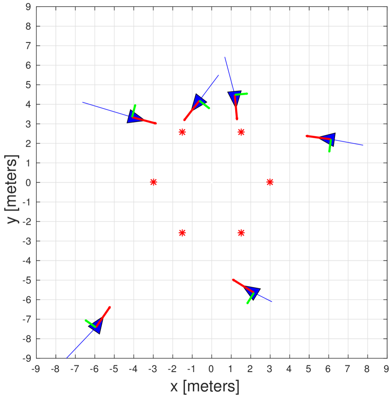
(a) formation control

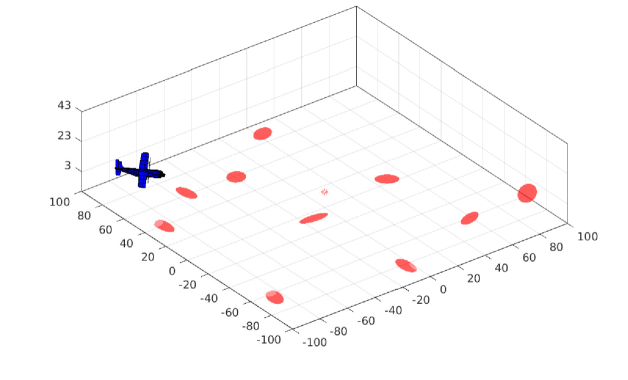
(b) robot navigation

Figure 2: Applications of the LQG control and sensing co-design framework.

V-A Sensing-constrained formation control

Simulation setup. The application scenario is illustrated in Fig. 2(a). A team of $n$ agents (blue triangles) moves in 2D. At $t=1$, the agents are randomly deployed in a $10\rm{m}\times 10\rm{m}$ square. Their objective is to reach a target formation shape (red stars); in Fig. 2(a) the desired formation has an hexagonal shape, while in general for a formation of $n$, the desired formation is an equilateral polygon with $n$ vertices. Each robot is modeled as a double-integrator, with state $x_{i}=[p_{i}\;v_{i}]^{\mathsf{T}}\in{{\mathbb{R}}^{4}}$ ($p_{i}$ is agent $i$’s position, and $v_{i}$ its velocity), and can control its acceleration $u_{i}\in{{\mathbb{R}}^{2}}$. The process noise is a diagonal matrix $W=\mathrm{diag}\left([1e^{-2},\;1e^{-2},\;1e^{-4},\;1e^{-4}]\right)$. Each robot $i$ is equipped with a GPS, which measures the agent position $p_{i}$ with a covariance $V_{gps,i}=2\cdot{\mathbf{I}}_{2}$. Moreover, the agents are equipped with lidars allowing each agent $i$ to measure the relative position of another agent $j$ with covariance $V_{lidar,ij}=0.1\cdot{\mathbf{I}}_{2}$. The agents have limited on-board resources, hence they want to activate only $k$ sensors.

For our tests, we consider two setups. In the first, named homogeneous formation control, the LQG weight matrix $Q$ is a block diagonal matrix with $4\times 4$ blocks, and each block $i$ chosen as $Q_{i}=0.1\cdot{\mathbf{I}}_{4}$; since each block of $Q$ weights equally the tracking error of a robot, in the homogeneous case the tracking error of all agents is equally important. In the second setup, named heterogeneous formation control, $Q$ is chose as above, except for one of the agents, say robot 1, for which we choose $Q_{1}=10\cdot{\mathbf{I}}_{4}$; this setup models the case in which each agent has a different role or importance, hence one weights differently the tracking error of the agents. In both cases the matrix $R$ is chosen to be the identity matrix. The simulation is carried on over $T$ time steps, and $T$ is also chosen as LQG horizon. Results are averaged over 100 Monte Carlo runs: at each run we randomize the initial estimation covariance $\Sigma_{1|1}$.

Compared techniques. We compare five techniques. All techniques use an LQG-based estimator and controller, and they only differ by the selections of the active sensors. The first approach is the optimal sensor selection, denoted as optimal, which attains the minimum in eq. (10), and which we compute by enumerating all possible subsets. The second approach is a pseudo-random sensor selection, denoted as random^∗, which selects all the GPS measurements and a random subset of the lidar measurements. The third approach, denoted as logdet, selects sensors so to minimize the average $\log\det$ of the estimation covariance over the horizon; this approach resembles [24] and is agnostic to the control task. The fourth approach is the proposed sensor selection strategy (Algorithm 2), and is denoted as s-LQG. Finally, we also report the LQG performance when all sensors are selected. This approach is denoted as allSensors.

Results. The results of the numerical analysis are reported in Fig. 3. When not specified otherwise, we consider a formation of $n=4$ agents, which can only use a total of $k=6$ sensors, and a control horizon $T=20$. Fig. 3(a) shows the LQG cost for the homogeneous case and for increasing horizon. We note that, in all tested instance, the proposed approach s-LQG matches the optimal selection optimal, and both approaches are relatively close to allSensors, which selects all the available sensors. On the other hand, logdet leads to worse tracking performance, and is often close to random^∗. These considerations are confirmed by the heterogeneous setup, in Fig. 3(b). In this case, the separation between our proposed approach and logdet becomes even larger; the intuition is that the heterogeneous case rewards differently the tracking errors at different agents, hence while logdet attempts to equally reduce the estimation error across the formation, the proposed approach s-LQG selects sensors in a task-oriented fashion, since the matrices $\Theta_{t}$ for all $t=1,2,\ldots,T$ in the cost function in eq. (10) incorporate the LQG weight matrices.

Fig. 3(c) shows the LQG cost attained for increasing number of selected sensors $k$ and for the homogeneous case. For increasing number of sensors all techniques converge to allSensors (since the entire ground set is selected). Fig. 3(d) shows the same statistics for the heterogeneous case. Now, s-LQG matches allSensors earlier, starting at $k=7$; intuitively, in the heterogeneous case, adding more sensors may have marginal impact on the LQG cost (e.g., if the cost rewards a small tracking error for robot 1, it may be of little value to take a lidar measurement between robot 3 and 4). This further stresses the importance of the proposed framework as a parsimonious way to control a system with minimal resources.

Fig. 3(e) and Fig. 3(f) show the LQG cost attained by the compared techniques for increasing number of agents. optimal quickly becomes intractable to compute, hence we omit values beyond $n=4$. In both figures, the separation among the techniques increases with the number of agents, since the set of available sensors quickly increases with $n$. In the heterogeneous case s-LQG remains relatively close to allSensors, implying that for the purpose of LQG control, using a cleverly selected small subset of sensors still ensures excellent tracking performance.

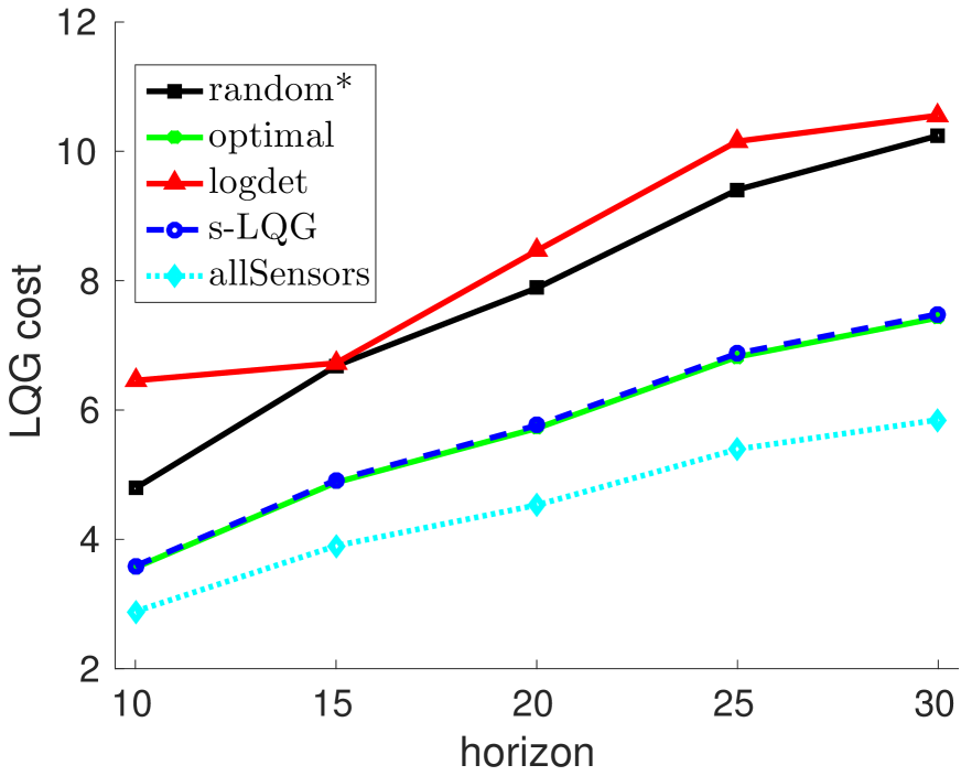
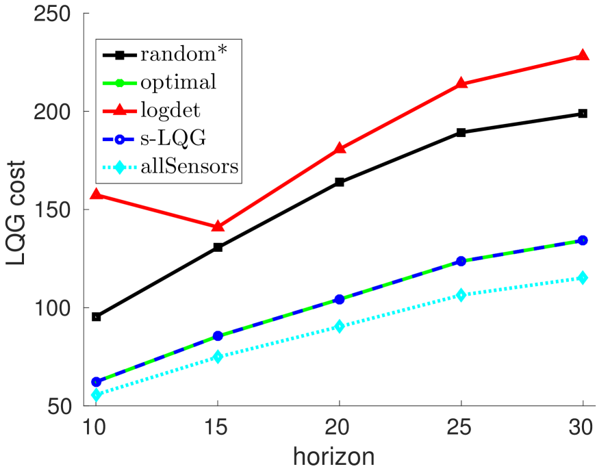
(a) homogeneous	(b) heterogeneous
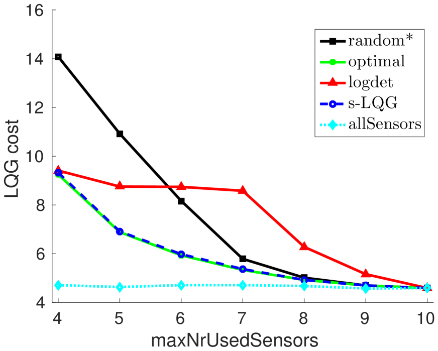
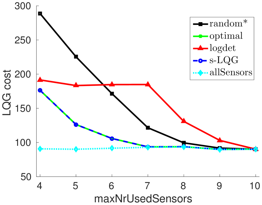
(c) homogeneous	(d) heterogeneous
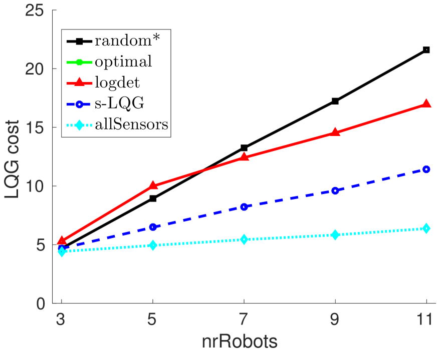
(e) homogeneous	(f) heterogeneous

Figure 3: LQG cost for increasing (a)-(b) control horizon $T$, (c)-(d) number of used sensors $k$ (all sensors are considered to have sensor-cost 1), and (e)-(f) number of agents $n$. Statistics are reported for the homogeneous formation control setup (left column), and the heterogeneous setup (right column).

V-B Resource-constrained robot navigation

Simulation setup. The second application scenario is illustrated in Fig. 2(b). An unmanned aerial robot (UAV) moves in a 3D space, starting from a randomly selected location. The objective of the UAV is to land, and specifically, to reach $[0,\;0,\;0]$ with zero velocity. The UAV is modeled as a double-integrator, with state $x=[p\;v]^{\mathsf{T}}\in{{\mathbb{R}}^{6}}$ ($p$ is the position, while $v$ its velocity), and can control its acceleration $u\in{{\mathbb{R}}^{3}}$. The process noise is $W={\mathbf{I}}_{6}$. The UAV is equipped with multiple sensors. It has an on-board GPS, measuring the UAV position $p$ with a covariance $2\cdot{\mathbf{I}}_{3}$, and an altimeter, measuring only the last component of $p$ (altitude) with standard deviation $0.5\rm{m}$. Moreover, the UAV can use a stereo camera to measure the relative position of $\ell$ landmarks on the ground; we assume the location of each landmark to be known approximately, and we associate to each landmark an uncertainty covariance (red ellipsoids in Fig. 2(b)), which is randomly generated at the beginning of each run. The UAV has limited on-board resources, hence it wants to use only a few of sensing modalities. For instance, the resource-constraints may be due to the power consumption of the GPS and the altimeter, or may be due to computational constraints that prevent to run multiple object-detection algorithms to detect all landmarks on the ground. We consider two sensing-constrained scenarios: (i) all sensors to have the same cost (equal to $1$), in which case, the UAV can activate at most $k$ sensors; (ii) the sensors to have heterogeneous costs: particularly, the GPS’s cost is set equal to $3$; the altimeter’s cost is set equal to 2; and each landmark’s cost is set equal to $1$.

We use $Q=\mathrm{diag}\left([1e^{-3},\;1e^{-3},\;10,\;1e^{-3},\;1e^{-3},\;10]\right)$ and $R={\mathbf{I}}_{3}$. The structure of $Q$ reflects the fact that during landing we are particularly interested in controlling the vertical direction and the vertical velocity (entries with larger weight in $Q$), while we are less interested in controlling accurately the horizontal position and velocity (assuming a sufficiently large landing site). In the following, we present results averaged over 100 Monte Carlo runs: in each run, we randomize the covariances describing the landmark position uncertainty.

Compared techniques. We consider the five techniques discussed in the previous section.

Results. The results of our numerical analysis are reported in Fig. 4 for the case where all sensors have the same sensor-cost, and in Fig. 5 for the case where sensors have different costs. When not specified otherwise, we consider a total of $k=3$ sensors to be selected, and a control horizon $T=20$.

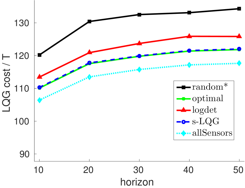
(a) heterogeneous

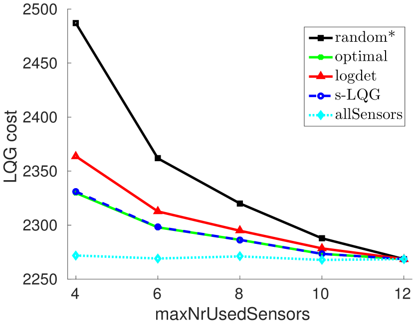
(b) heterogeneous

Figure 4: LQG cost for increasing (a) horizon $T$​, and (b) number of used sensors $k$ (all sensors are considered to have cost 1).

In Fig. 4(a) we plot the LQG cost normalized by the horizon, which makes more visible the differences among the techniques. Similarly to the formation control example, s-LQG matches the optimal selection optimal, while logdet and random^∗ have suboptimal performance. Fig. 4(b) shows the LQG cost attained by the compared techniques for increasing number of selected sensors $k$. All techniques converge to allSensors for increasing $k$, but in the regime in which few sensors are used s-LQG still outperforms alternative sensor selection schemes, and matches optimal.

Fig. 5 shows the LQG cost attained by the compared techniques for increasing control horizon and various sensor cost budgets $b$. Similarly to Fig. 4, s-LQG has the same performance as optimal, whereas logdet and random^∗ have suboptimal performance. Notably, for $b=15$ all sensors can be chosen; for this reason in Fig. 5(d) all compared techniques (but the random) have the same performance.

VI Concluding Remarks

We addressed an LQG control and sensing co-design problem, where one jointly designs control and sensing policies under resource constraints. The problem is central in modern IoT and IoBT control applications, ranging from large-scale networked systems to miniaturized robotic networks. Motivated by the inapproximability of the problem, we provided the first scalable algorithms with per-instance suboptimality bounds. Importantly, the bounds are non-vanishing under general control-theoretic conditions, encountered in most real-world systems. To this end, we also extended the literature on supermodular optimization: by providing scalable algorithms for optimizing approximately supermodular functions subject to heterogeneous cost constraints; and by providing novel suboptimality bounds that improve the known bounds even for exactly supermodular optimization.

The paper opens several avenues for future research. First, the development of distributed implementations of the proposed algorithms would offer computational speedups. Second, other co-design problems are interesting to be explored, such as the co-design of control-sensing-actuation. Third, while we provide bounds on an approximate sensor design against optimal design, one could provide bounds against the case where all sensors are used [68]. Finally, in adversarial or failure-prone scenarios, one must account for sensor failures; to this end, one could leverage recent results on robust combinatorial optimization [69].

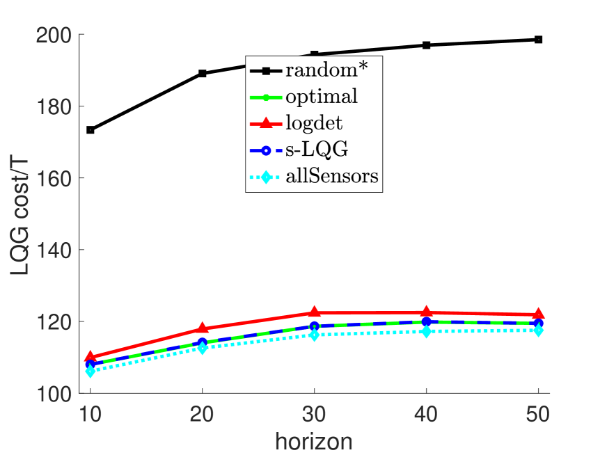
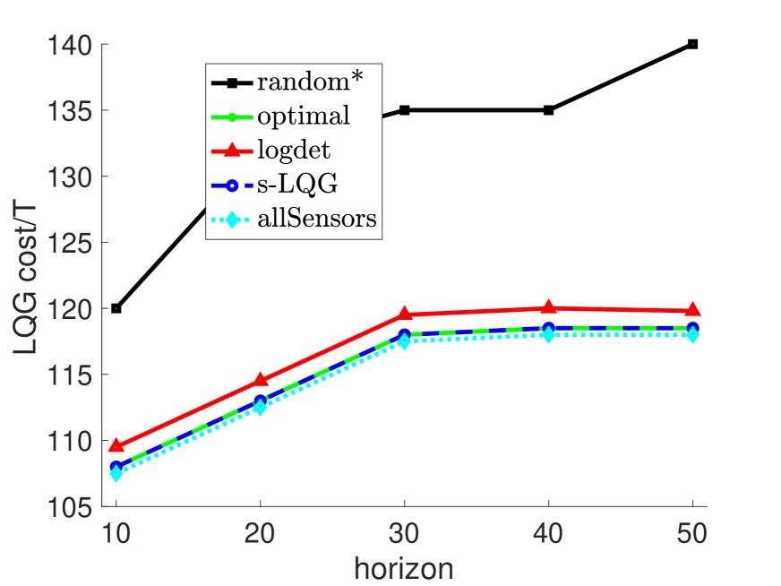
(a) budget $b=6$	(b) budget $b=8$
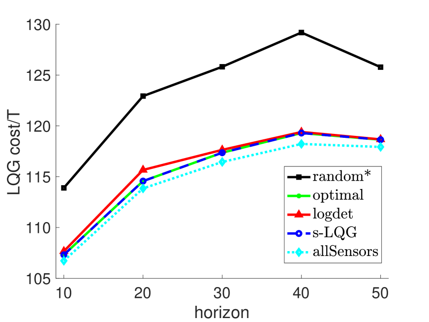
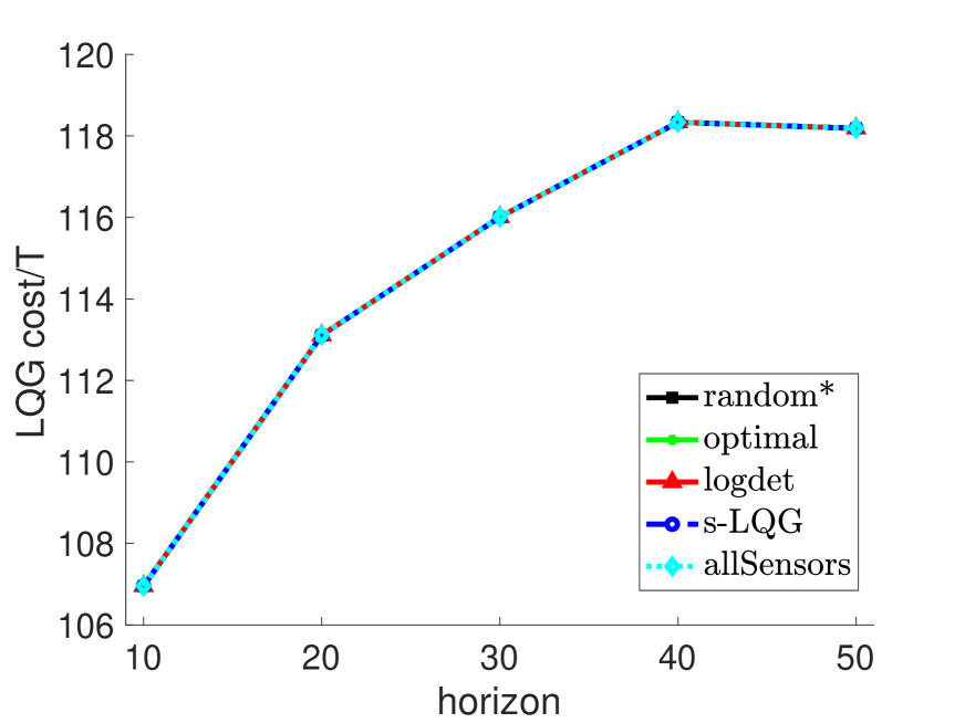
(c) budget $b=10$	(d) budget $b=15$

Figure 5: LQG cost for increasing horizon $T$ and for various sensing budgets $b$.

Appendix A: Preliminary facts

Lemma 1 ([70, Proposition 8.5.5]).

Consider two positive definite matrices $A_{1}$ and $A_{2}$. If $A_{1}\preceq A_{2}$, then $A_{2}^{-1}\preceq A_{1}^{-1}\!$.

Lemma 2 (Trace inequality [70, Proposition 8.4.13]).

Consider a symmetric $A$, and a positive semi-definite $B$. Then,

$$\lambda_{\min}(A)\textrm{tr}\left(B\right)\leq\textrm{tr}\left(AB\right)\leq\lambda_{\max}(A)\textrm{tr}\left(B\right).$$

Lemma 3 (Woodbury identity [70, Corollary 2.8.8]).

Consider $A$, $C$, $U$ and $V$ such that $A$, $C$, and $A+UCV$ are invertible. Then,

$$(A+UCV)^{-1}=A^{-1}-A^{-1}U(C^{-1}+VA^{-1}U)^{-1}VA^{-1}\!.$$

Lemma 4 ([70, Proposition 8.5.12]).

Consider two symmetric matrices $A_{1}$ and $A_{2}$, and a positive semi-definite matrix $B$. If $A_{1}\preceq A_{2}$, then $\textrm{tr}\left(A_{1}B\right)\leq\textrm{tr}\left(A_{2}B\right)$.

Lemma 5 ([1, Appendix E]).

For any sensors ${\cal S}$, $\Sigma_{t|t}({\cal S})$ is the solution of the Kalman filtering recursion

$$\begin{array}[]{rcl}\Sigma_{t|t}({\cal S})\!\!&\!\!=\!\!&\!\![\Sigma_{t|t-1}({\cal S})^{-1}+C_{t}({\cal S})^{\mathsf{T}}V_{t}({\cal S})^{-1}C_{t}({\cal S})]^{-1}\!,\\ \Sigma_{t+1|t}({\cal S})\!\!&\!\!=\!\!&\!\!A_{t}\Sigma_{t|t}({\cal S})A_{t}^{\mathsf{T}}+W_{t},\end{array}$$ (22)

with boundary condition $\Sigma_{1|1}({\cal S})=\Sigma_{1|1}$.

Lemma 6 ([64, Lemma 6]).

Consider two sensor sets ${\cal S}_{1},{\cal S}_{2}\subseteq{\cal V}$. If ${\cal S}_{1}\subseteq{\cal S}_{2}$, then $\Sigma_{1|1}({\cal S}_{1})\succeq\Sigma_{1|1}({\cal S}_{2})$.

Lemma 7 ([64, Corollary 1]).

Let $\Sigma_{t|t}$ be defined as in eq. (22) with boundary condition $\Sigma_{1|1}$; similarly, let $\bar{\Sigma}_{t|t}$ be defined as in eq. (22) with boundary condition $\bar{\Sigma}_{1|1}$. If $\Sigma_{t|t}\preceq\bar{\Sigma}_{t|t}$, then $\Sigma_{t+i|t+i}\preceq\bar{\Sigma}_{t+i|t+i}$ for any positive integer $i$.

Lemma 8 ([64, Corollary 2]).

Let $\Sigma_{t|t}$ be defined as in eq. (22) with boundary condition $\Sigma_{1|1}$; similarly, let $\bar{\Sigma}_{t|t}$ be defined as in eq. (22) with boundary condition $\bar{\Sigma}_{1|1}$. If $\Sigma_{t|t}\preceq\bar{\Sigma}_{t|t}$, then $\Sigma_{t+i|t+i-1}\preceq\bar{\Sigma}_{t+i|t+i-1}$ for any positive integer $i$.

Lemma 9.

Consider positive real numbers $a$, $b$, $\gamma$, $a_{1},a_{2},\ldots,a_{n}$ such that $\sum_{i=1}^{n}a_{i}=a$. Then,

$$f(a_{1},a_{2},\ldots,a_{n})=1-\prod_{i=1}^{n}\left(1-\gamma\frac{a_{i}}{b}\right)$$

has its minimum at $a_{1}=a_{2}=\ldots=a_{n}=a/n$, and

$$f(a/n,a/n,\ldots,a/n)=1-\left(1-{\frac{a\gamma}{bn}}\right)^{n}\geq 1-e^{-a\gamma/b}\!.$$

Proof of Lemma 9.

The proof is obtained using the method of Lagrange multipliers, and is omitted (for a complete proof, see [65, Proof of Lemma 9]) ∎

Lemma 10 (Monotonicity of cost function in eq. (10) [64, Proposition 2]).

Consider $\sum_{t=1}^{T}\textrm{tr}\left(\Theta_{t}\Sigma_{t|t}({\cal S})\right)$ in eq. (10). If ${\cal S}_{1}\subseteq{\cal S}_{2}$, then $\sum_{t=1}^{T}\textrm{tr}\left(\Theta_{t}\Sigma_{t|t}({\cal S}_{1})\right)\geq\sum_{t=1}^{T}\textrm{tr}\left(\Theta_{t}\Sigma_{t|t}({\cal S}_{2})\right)$.

Appendix B: Proof of Theorem 1

B.1. Proof of part (1) of Theorem 1

Lemma 11.

Consider any ${\cal S}$, and let ${u^{\star}_{1:T}({\cal S})}$ be the vector of control policies $(K_{1}\hat{x}_{1}({\cal S}),K_{2}\hat{x}_{2}({\cal S}),\ldots,K_{T}\hat{x}_{T}({\cal S}))$. Then $u^{\star}_{1:T}({\cal S})$ is an optimal control policy:

$$u^{\star}_{1:T}({\cal S})\in\operatorname*{arg\,min}_{u_{1:T}({\cal S})}h[{\cal S},u_{1:T}({\cal S})],$$ (23)

and, particularly, $u^{\star}_{1:T}({\cal S})$ attains an LQG cost equal to:

$$h[{\cal S},u^{\star}_{1:T}({\cal S})]=\mathbb{E}(\|x_{1}\|_{N_{1}})+\sum_{t=1}^{T}\left\{\text{tr}[\Theta_{t}\Sigma_{t|t}({\cal S})]+\textrm{tr}\left(W_{t}S_{t}\right)\right\}.$$ (24)

Proof of Lemma 11.

The proof follows Lemma 1’s proof in [20], and can also be found in [65, Appendix B]. ∎

Proof of part (1) of Theorem 1.

Eq. (10) is a direct consequence of eq. (24), since the value of Problem 1 is equal to $\min_{{\cal S}\subseteq{\cal V},c({\cal S})\leq b}h[{\cal S},u^{\star}_{1:T}({\cal S})]$, and both $\mathbb{E}(\|x_{1}\|_{N_{1}})=\textrm{tr}\left(\Sigma_{1|1}N_{1}\right)$ and $\sum_{t=1}^{T}\textrm{tr}\left(W_{t}S_{t}\right)$ are independent of ${\cal S}$. Finally, eq. (11) directly follows from eq. (23).

∎

B.1. Proof of part (2) of Theorem 1

Lemma 12.

${\cal S}^{\star}$, and $u^{\star}_{1:T}$ are a solution to Problem 2 if and only if they are a solution to

$$\min_{\scriptsize{\cal S}\subseteq{\cal V},u_{1:T}({\cal S})}c({\cal S}){,\;\;\rm{s.t.}}\;\;\min_{\scriptsize u_{1:T}({{\cal S}})}h\left[{{\cal S}},u_{1:T}({{\cal S}})\right]\leq\kappa.$$ (25)

Proof of Lemma 12.

We prove the lemma by contradiction. Particularly, let ${\cal S}^{\star}$ and $u^{\star}_{1:T}$ be a solution to Problem 2, and assume by contradiction that they are not to eq. (25), which instead has solution $\widehat{{\cal S}}$ and $\widehat{u}_{1:T}$. By optimality of $\widehat{{\cal S}}$ and $\widehat{u}_{1:T}$ (and suboptimality of ${\cal S}^{\star}$ and $u^{\star}_{1:T}$) in eq. (25), it follows $c(\widehat{{\cal S}})<c({\cal S}^{\star})$. In addition, $g(\widehat{{\cal S}})\leq\kappa$, since $(\widehat{{\cal S}},{\widehat{u}_{1:T}})$ must be feasible for eq. (25). However, the latter implies $h\left(\widehat{{\cal S}},{\widehat{u}_{1:T}}\right)\leq\kappa$. Therefore, $(\widehat{{\cal S}},{\widehat{u}_{1:T}})$ is feasible for Problem 2 and has a better objective value with respect to the optimal solution $({\cal S}^{\star},u^{\star}_{1:T})$ (we already observed $c(\widehat{{\cal S}})<c({\cal S}^{\star})$), leading to contradiction.

For the other direction, now let ${\cal S}^{\star}$ and ${u^{\star}_{1:T}}$ be a solution to eq. (25), and assume that they are not to Problem 2, which instead has solution $(\widehat{{\cal S}},\widehat{u}_{1:T})$. By optimality of $(\widehat{{\cal S}},\widehat{u}_{1:T})$ (and suboptimality of ${\cal S}^{\star}$ and $u^{\star}_{1:T}$) in Problem 2, it follows $c(\widehat{{\cal S}})<c({\cal S}^{\star})$. In addition, $h\left(\widehat{{\cal S}},{\widehat{u}_{1:T}}\right)\leq\kappa$, since $(\widehat{{\cal S}},{\widehat{u}_{1:T}})$ must be feasible for Problem 2, and, as a result, $g(\widehat{{\cal S}})\leq\kappa$. Therefore, $(\widehat{{\cal S}},{\widehat{u}_{1:T}})$ is feasible for eq. (25) and has a better objective value with respect to the optimal solution $({\cal S}^{\star},u^{\star}_{1:T})$ (we already observed $c(\widehat{{\cal S}})<c({\cal S}^{\star})$), leading to contradiction. ∎

Proof of part (2) of Theorem 1.

The proof follows from Lemma 11 and Lemma 12. ∎

Appendix C: Proof of Theorem 2

Consider a problem instance for Problem 1 and Problem 2, where $T=1$, and $A_{1}=B_{1}=C_{1}=Q_{1}=R_{1}=I$. Then, $\Theta_{1}={\mathbf{I}}/2$, and, as a result, the objective function in eq. (10) becomes $1/2\text{tr}[\Sigma_{1|1}({\cal S})]$. Now, choosing $\Sigma_{1|1}({\cal S})$ to be the steady state Kalman filtering matrix defined in [66, Theorem 2], as well as, $c({\cal S})$, $b$ be as in [66, Theorem 2], makes eq. (10) and the optimization problem in [66] equivalent. But, the latter is inapproximable in polynomial time [66, Theorem 2] (namely, unless NP$=$P, there is no polynomial time algorithm that guarantees a constant suboptimality bound). Therefore, eq. (10) is too, and due to Theorem 1 both Problem 1 and Problem 2 as well.

Appendix D: Proof of Theorem 3

For any ${\cal S}$, let $f({\cal S})\triangleq\sum_{t=1}^{T}\text{tr}[\Theta_{t}\Sigma_{t|t}({\cal S})]$ be the objective function in eq. (10), ${\cal S}^{\star}$ be a solution in eq. (10), and $b^{\star}\triangleq c({\cal S}^{\star})$. Let $\widehat{{\cal S}}_{2}$ be the set Algorithm 2 constructs by the end of line 21; let ${\cal G}\triangleq\widehat{{\cal S}}_{2}$. Let $s_{i}$ be the $i$-th element added in ${\cal G}$ during the $i$-th iteration of Algorithm 2’s “while loop” (lines 5-18). Let ${\cal G}_{i}\triangleq\{s_{1},s_{2},\ldots,s_{i}\}$. Finally, consider Algorithm 2’s “while loop” terminates after $l+1$ iterations.

Algorithm 2’s “while loop” terminates: (i) when ${\cal V}^{\prime}=\emptyset$, that is, when all available sensors in ${\cal V}$ can been chosen by Algorithm 2 as active while satisfying the budget constraint $b$; and (ii) when $c({\cal G}_{l+1})>b$, that is, when the addition of $s_{l+1}$ in ${\cal G}_{l}$ makes the cost of ${\cal G}_{l+1}$ to violate the budget $b$. Henceforth, we focus on the second scenario, which implies $s_{l+1}$ will be removed by the “if” statement in Algorithm 2’s lines 19–21 and, as a result, ${\cal G}_{l}=\widehat{{\cal S}}_{2}$.

Lemma 13 (Generalization of [51, Lemma 2]).

For $i=1,2,\ldots,l+1$, it holds

$$f({\cal G}_{i-1})-f({{\cal G}}_{i})\geq\frac{\gamma_{f}c(s_{i})}{b^{\star}}(f({{\cal G}}_{i-1})-f({\cal S}^{\star})).$$

Proof of Lemma 13.

Due to the monotonicity of the cost function $f$ in eq. (10) (Lemma 10),

$$f({\cal G}_{i-1})-f({\cal S}^{\star}) \leq f({\cal G}_{i-1})-f({\cal S}^{\star}\cup{\cal G}_{i-1})$$

$$=f({\cal G}_{i-1})-f[({\cal S}^{\star}\setminus{\cal G}_{i-1})\cup{\cal G}_{i-1}].$$

Let $\{z_{1},z_{2},\ldots,z_{m}\}\triangleq{\cal S}^{\star}\setminus{\cal G}_{i-1}$, and also let

$$d_{j}\triangleq f({\cal G}_{i-1}\cup\{z_{1},z_{2},\ldots,z_{j-1}\})-f({\cal G}_{i-1}\cup\{z_{1},z_{2},\ldots,z_{j}\}),$$

for $j=1,2,\ldots,m$. Then, $f({\cal G}_{i-1})-f({\cal S}^{\star})\leq\sum_{j=1}^{m}d_{j}$. Now,

$$\frac{d_{j}}{c(z_{j})}\leq\frac{f({\cal G}_{i-1})-f({\cal G}_{i-1}\cup\{z_{j}\})}{\gamma_{f}c(z_{j})}\leq\frac{f({\cal G}_{i-1})-f({\cal G}_{i})}{\gamma_{f}c(s_{i})},$$

where the first inequality holds due to the Definition 3 of $\gamma_{f}$, and the second due to the greedy rule (Algorithm 2’s line 15) and the definitions of ${\cal G}_{i}$, and $s_{i}$. Since $\sum_{j=1}^{m}c(z_{j})\leq b^{\star}$,

$$f({\cal G}_{i-1})-f({\cal S}^{\star})\leq\sum_{j=1}^{m}d_{j}\leq b^{\star}\frac{f({\cal G}_{i-1})-f({\cal G}_{i})}{\gamma_{f}c(s_{i})}.$$

∎

Lemma 14 (Adapation of [51, Lemma 3]).

For $i=1,2,\ldots,l+1$,

$$f(\emptyset)-f(G_{i})\geq\left[1-\prod_{j=1}^{i}\left(1-\frac{\gamma_{f}c(s_{j})}{b^{\star}}\right)\right][f(\emptyset)-f({\cal S}^{\star})].$$

Proof of Lemma 14.

We complete the proof inductively. For $i=1$, we need to prove $f(\emptyset)-f(G_{1})\geq\gamma_{f}c(s_{1})/b^{\star}[f(\emptyset)-f({\cal S}^{\star})]$, which follows from Lemma 13 for $i=1$. Then, for $i>1$,

$$f(\emptyset)-f({\cal G}_{i}) =f(\emptyset)-f({\cal G}_{i-1})+[f({\cal G}_{i-1})-f({\cal G}_{i})]$$

$$\geq f(\emptyset)-f({\cal G}_{i-1})+$$

$$\;\;\;\;\frac{\gamma_{f}c(s_{i})}{b^{\star}}(f(G_{i-1})-f({\cal S}^{\star}))$$

$$=\left(1-\frac{\gamma_{f}c(s_{i})}{b^{\star}}\right)[f(\emptyset)-f({\cal G}_{i-1}])+$$

$$\;\;\;\;\frac{\gamma_{f}c(s_{i})}{b^{\star}}[f(\emptyset)-f({\cal S}^{\star})]$$

$$\geq\left(1-\frac{\gamma_{f}c(s_{i})}{b^{\star}}\right)\left[1-\prod_{j=1}^{i-1}\left(1-\frac{\gamma_{f}c(s_{j})}{b^{\star}}\right)\right]$$

$$\;\;\;\;[f(\emptyset)-f({\cal S}^{\star})]+\frac{\gamma_{f}c(s_{i})}{b^{\star}}[f(\emptyset)-f({\cal S}^{\star})]$$

$$=\left[1-\prod_{j=1}^{i}\left(1-\frac{\gamma_{f}c(s_{j})}{b^{\star}}\right)\right][f(\emptyset)-f({\cal S}^{\star})],$$

where we used Lemma 13 for the first inequality, and the induction hypothesis for the second. ∎

Proof of part (1) of Theorem 3.

To prove Algorithm 1’s approximation bound $\gamma_{g}/2\left(1-e^{-\gamma_{g}}\right)$, we let $b^{\prime}\triangleq{\sum_{j=1}^{l+1}c(s_{j})}$. Then,

$$f(\emptyset)-f({\cal G}_{l+1}) \geq\left[1-\prod_{j=1}^{l+1}\left(1-\frac{\gamma_{f}c(s_{j})}{b^{\star}}\right)\right][f(\emptyset)-f({\cal S}^{\star})]$$

$$\geq\left(1-e^{-\gamma_{f}b^{\prime}/b^{\star}}\right)[f(\emptyset)-f({\cal S}^{\star})],$$

$$\geq\left(1-e^{-\gamma_{f}}\right)[f(\emptyset)-f({\cal S}^{\star})],$$ (26)

where the first inequality follows from Lemma 14, the second from Lemma 9, and ineq. (26) from that $b^{\prime}/b^{\star}\geq 1$ and, as a result, $e^{-\gamma_{f}b^{\prime}/b^{\star}}\leq e^{-\gamma_{f}}$​, that is, $1-e^{-\gamma_{f}b^{\prime}/b^{\star}}\geq 1-e^{-\gamma_{f}}$​.

Also, $f(\emptyset)-f(\widehat{{\cal S}}_{1})\geq\gamma_{f}[f({\cal G}_{l})-f({\cal G}_{l+1})]$ due to the Definition 3 of $\gamma_{g}$ and, as a result,

$$\!\!\!\gamma_{f}[f(\emptyset)-f({\cal G}_{l+1})]$$

$$\leq f(\emptyset)-f(\widehat{{\cal S}}_{1})+\gamma_{f}[f(\emptyset)-f({\cal G}_{l})]$$

$$\leq 2\max\left\{f(\emptyset)-f(\widehat{{\cal S}}_{1}),\gamma_{f}[f(\emptyset)-f({\cal G}_{l})]\right\}.$$ (27)

Substituting ineq. (26) in ineq. (27), and rearranging, gives

$$\!\!\!\max\left\{f(\emptyset)-f(\widehat{{\cal S}}_{1}),\gamma_{f}[f(\emptyset)-f({\cal G}_{l})]\right\}$$

$$\geq\frac{\gamma_{f}}{2}\left(1-e^{-\gamma_{f}}\right)[f(\emptyset)-f({\cal S}^{\star})],$$

which implies (since $\gamma_{f}$ takes values in $[0,1]$)

$$\!\!\!\max\left[f(\emptyset)-f(\widehat{{\cal S}}_{1}),f(\emptyset)-f({\cal G}_{l})\right]$$

$$\geq\frac{\gamma_{f}}{2}\left(1-e^{-\gamma_{f}}\right)[f(\emptyset)-f({\cal S}^{\star})].$$ (28)

Finally, the bound $\gamma_{g}/2\left(1-e^{-\gamma_{g}}\right)$ follows from ineq. (28) as the combination of the following three observations: i) ${\cal G}_{l}=\widehat{{\cal S}}_{2}$, and, as a result, $f(\emptyset)-f({\cal G}_{l})=f(\emptyset)-f(\widehat{{\cal S}}_{2})$. ii) Algorithm 2 returns $\widehat{{\cal S}}$ such at $\widehat{{\cal S}}\in\arg\max_{{\cal S}\in\{\widehat{{\cal S}}_{1},\widehat{{\cal S}}_{2}\}}\left[f(\emptyset)-f({\cal S})\right]$ and, as a result, the previous observation, along with ineq. (28), gives:

$$f(\emptyset)-f(\widehat{{\cal S}})\geq\frac{\gamma_{f}}{2}\left(1-e^{-\gamma_{f}}\right)[f(\emptyset)-f({\cal S}^{\star})].$$ (29)

iii) Finally, Lemma 11 implies that for any ${\cal S},{\cal S}^{\prime}$, $g({\cal S})=f({\cal S})+\mathbb{E}(\|x_{1}\|_{N_{1}})+\sum_{t=1}^{T}\textrm{tr}\left(W_{t}S_{t}\right)$, where $\mathbb{E}(\|x_{1}\|_{N_{1}})+\sum_{t=1}^{T}\textrm{tr}\left(W_{t}S_{t}\right)$ is independent of ${\cal S}$. As a result, for any ${\cal S},{\cal S}^{\prime}\subseteq{\cal V}$, then $f({\cal S})-f({\cal S}^{\prime})=g({\cal S})-g({\cal S}^{\prime})$, which implies $\gamma_{f}=\gamma_{g}$ due to Definition 3. In addition, Lemma 11 implies for any ${\cal S}\subseteq{\cal V}$ that $g({\cal S})=h[{\cal S},u_{1:T}({{\cal S}})]$ and $g^{\star}=g({\cal S}^{\star})$. Thereby, for any ${\cal S}$ that $f(\emptyset)-f({\cal S})=g(\emptyset)-g({\cal S})=h[\emptyset,u_{1:T}(\emptyset)]-h[{\cal S},u_{1:T}({{\cal S}})]$ and $f(\emptyset)-f({\cal S}^{\star})=g(\emptyset)-g({\cal S}^{\star})=h[\emptyset,u_{1:T}(\emptyset)]-g^{\star}$​​. Overall, ineq. (29) is written as

$$h[\emptyset,u_{1:T}(\emptyset)]-h[\widehat{{\cal S}},u_{1:T}({\widehat{{\cal S}}})]\geq$$

$$\qquad\qquad\qquad\frac{\gamma_{f}}{2}\left(1-e^{-\gamma_{f}}\right)\left\{h[\emptyset,u_{1:T}(\emptyset)]-g^{\star}\right\},$$

which implies the bound $\gamma_{g}/2\left(1-e^{-\gamma_{g}}\right)$.

It remains to prove $1-e^{-\gamma_{g}c(\widehat{{\cal S}})/b}$:

$$f(\emptyset)-f({\cal G}_{l}) \geq\left[1-\prod_{j=1}^{l}\left(1-\frac{\gamma_{f}c(s_{j})}{b^{\star}}\right)\right][f(\emptyset)-f({\cal G}_{l})]$$

$$\geq\left(1-e^{-\gamma_{f}c({\cal G}_{l})/b^{\star}}\right)[f(\emptyset)-f({\cal S}^{\star})],$$

$$\geq\left(1-e^{-\gamma_{f}c({\cal G}_{l})/b}\right)[f(\emptyset)-f({\cal S}^{\star})],$$ (30)

where the first inequality follows from Lemma 14, the second from Lemma 9, and ineq. (30) from that $c({\cal G}_{l})/b^{\star}\geq c({\cal G}_{l})/b$, since $b^{\star}\leq b$, which implies $e^{-\gamma_{f}c({\cal G}_{l})/b^{\star}}\leq e^{-\gamma_{f}c({\cal G}_{l})/b}$, i.e., $1-e^{-\gamma_{f}b^{\prime}/b^{\star}}\geq 1-e^{-\gamma_{f}c({\cal G}_{l})/b}$. The proof is completed using the observations (i)-(iii) above for $\gamma_{g}/2\left(1-e^{-\gamma_{g}}\right)$. ∎

Proof of part (2) of Theorem 3.

The proof is parallel to that of Theorem 2 in [71]. ∎

Appendix E: Proof of Theorem 4

We consider the notation in Appendix D. Also, let ${\cal S}^{\star}$ be a solution to Problem 2, and $b^{\star}=c({\cal S}^{\star})$. Consider the computation of the set $\widehat{{\cal S}}$ in Algorithm 4, and let ${\cal G}\triangleq\widehat{{\cal S}}$ be the returned one. Let $s_{i}$ be the $i$-th element added in ${\cal G}$ during the $i$-th iteration of Algorithm 4’s “while loop.” Finally, let ${\cal G}_{i}\triangleq\{s_{1},s_{2},\ldots,s_{i}\}$.

Lemma 15 (Adaptation of Lemma 13).

For $i=1,2,\ldots,|{\cal G}|$,

$$f({\cal G}_{i-1})-f(G_{i})\geq\frac{\gamma_{f}c(s_{i})}{b^{\star}}(f(G_{i-1})-f({\cal S}^{\star})).$$

Proof.

The proof is parallel to Lemma 13’s proof. ∎

Lemma 16 (Adaptation of Lemma 14).

For $i=1,2,\ldots,|{\cal G}|$,

$$f(\emptyset)-f(G_{i})\geq\left[1-\prod_{j=1}^{i}\left(1-\frac{\gamma_{f}c(s_{j})}{b^{\star}}\right)\right][f(\emptyset)-f({\cal S}^{\star})].$$

Proof.

The proof is parallel to Lemma 14’s proof. ∎

Proof of part (1) of Theorem 4.

We first observe ineq. (18) holds since Algorithm 3 returns $\widehat{{\cal S}}$ once $h[\widehat{{\cal S}},u_{1:T}(\widehat{{\cal S}})]\leq\kappa$ is satisfied.

It remains to prove ineq. (19). Let $l\triangleq|{\cal G}|$; then, ${\cal G}_{l}={\cal G}$, by the definition of ${\cal G}_{i}$, and from Lemma 14 for $i=l-1$,

$$f(\emptyset)-f({\cal G}_{l-1}) \geq\left[1-\prod_{j=1}^{l-1}\left(1-\frac{\gamma_{f}c(s_{j})}{b^{\star}}\right)\right][f(\emptyset)-f({\cal S}^{\star})]$$

$$\geq\left(1-e^{-\gamma_{f}c({\cal G}_{l-1})/b^{\star}}\right)[f(\emptyset)-f({\cal S}^{\star})],$$ (31)

where ineq. (31) follows from Lemma 9. Moreover, Lemma 11 implies that for any ${\cal S},{\cal S}^{\prime}$, it is $g({\cal S})=f({\cal S})+\mathbb{E}(\|x_{1}\|_{N_{1}})+\sum_{t=1}^{T}\textrm{tr}\left(W_{t}S_{t}\right)$, where $\mathbb{E}(\|x_{1}\|_{N_{1}})+\sum_{t=1}^{T}\textrm{tr}\left(W_{t}S_{t}\right)$ is independent of ${\cal S}$, and, as a result, $f({\cal S})-f({\cal S}^{\prime})=g({\cal S})-g({\cal S}^{\prime})$, which implies $\gamma_{f}=\gamma_{g}$. Moreover, Lemma 11 implies for any ${\cal S}\subseteq$ that $g({\cal S})=h[{\cal S},u_{1:T}({{\cal S}})]$, and, as a result, $f(\emptyset)-f({\cal G}_{l-1})=h[\emptyset,u_{1:T}(\emptyset)]-h[{\cal G}_{l-1},u_{1:T}({\cal G}_{l-1})]$ and $f(\emptyset)-f({\cal S}^{\star})=h[\emptyset,u_{1:T}(\emptyset)]-h[{\cal S}^{\star},u_{1:T}({\cal S}^{\star})]$. In sum, ineq. (31) is the same as the inequality

$$h[\emptyset,u_{1:T}(\emptyset)]-h[{\cal G}_{l-1},u_{1:T}({\cal G}_{l-1})]\geq$$

$$\;\;\;\left(1-e^{-\gamma_{g}c({\cal G}_{l-1})/b^{\star}}\right)\left\{h[\emptyset,u_{1:T}(\emptyset)]-h[{\cal S}^{\star},u_{1:T}({\cal S}^{\star})]\right\},$$

which, by letting ${{\beta}}\triangleq 1-e^{-\gamma_{g}c({\cal G}_{l-1})/b^{\star}}$ and rearranging, gives

$$h[{\cal G}_{l-1},u_{1:T}({\cal G}_{l-1})] \leq(1-{{\beta}})h[\emptyset,u_{1:T}(\emptyset)]+{{\beta}}h[{\cal S}^{\star}\!\!,u_{1:T}({\cal S}^{\star})]$$

$$\leq(1-{{\beta}})h[\emptyset,u_{1:T}(\emptyset)]+{{\beta}}\kappa,$$ (32)

where the second inequality holds because ${\cal S}^{\star}$ is a solution to Problem 2 and, as result, $h[{\cal S}^{\star}\!\!,u_{1:T}({\cal S}^{\star})]\leq\kappa$. Now, we recall Algorithm 4 returns ${\cal G}={\cal G}_{l}$ when for $i=l$ it is the first time $h[{\cal G}_{i},u_{1:T}({\cal G}_{i})]\leq\kappa$. Therefore, $h[{\cal G}_{l-1},u_{1:T}({\cal G}_{l-1})]>\kappa$ and, as a result, there exists $\epsilon>0$ such that $h[{\cal G}_{l-1},u_{1:T}({\cal G}_{l-1})]=(1+\epsilon)\kappa$, and ineq. (32) gives

$$(1+\epsilon)\kappa\leq(1-{{\beta}})h[\emptyset,u_{1:T}(\emptyset)]+{{\beta}}\kappa\Rightarrow$$

$$\epsilon\kappa\leq(1-{{\beta}})h[\emptyset,u_{1:T}(\emptyset)]-(1-{{\beta}})\kappa\Rightarrow$$

$$\epsilon\kappa\leq(1-{{\beta}})\{h[\emptyset,u_{1:T}(\emptyset)]-\kappa\}\Rightarrow$$

$$\epsilon\kappa\leq e^{-\gamma_{g}c({\cal G}_{l-1})/b^{\star}}\{h[\emptyset,u_{1:T}(\emptyset)]-\kappa\}\Rightarrow$$

$$\log\left(\frac{\epsilon\kappa}{h[\emptyset,u_{1:T}(\emptyset)]-\kappa}\right)\leq-\gamma_{g}c({\cal G}_{l-1})/b^{\star}\Rightarrow$$

$$c({\cal G}_{l-1})\leq\frac{1}{\gamma_{g}}\log\left(\frac{h[\emptyset,u_{1:T}(\emptyset)]-\kappa}{\epsilon\kappa}\right)b^{\star}\Rightarrow$$

$$c({\cal G})\leq c(s_{l})+\frac{1}{\gamma_{g}}\log\left(\frac{h[\emptyset,u_{1:T}(\emptyset)]-\kappa}{\epsilon\kappa}\right)b^{\star}\!\!,$$

where the latter holds since ${\cal G}={\cal G}_{l-1}\cup\{s_{l}\}$, due to the definitions of ${\cal G}$, ${\cal G}_{l-1}$, and $s_{l}$, and since $c({\cal G})=c({\cal G}_{l-1})+c(s_{l})$. Finally, since the definition of $\epsilon$ implies $\epsilon\kappa=h[{\cal G}_{l-1},u_{1:T}({\cal G}_{l-1})]-\kappa$, and the definition of ${\cal G}$ is ${\cal G}=\widehat{{\cal S}}$, the proof of ineq. (18) is complete. ∎

Proof of part (2) of Theorem 4.

The proof is similar to the proof of part (2) of Theorem 3. ∎

Appendix F: Proof of Theorem 5

We complete the proof by first deriving a lower bound for the numerator of $\gamma_{g}$, and then, by deriving an upper bound for the denominator $\gamma_{g}$. We use the following notation: $c\triangleq\mathbb{E}(x_{1}^{\mathsf{T}}N_{1}x_{1})+\sum_{t=1}^{T}\textrm{tr}\left(W_{t}S_{t}\right)$, and for any ${\cal S}$, and time $t=1,2,\ldots,T$, $f_{t}({\cal S})\triangleq\textrm{tr}\left(\Theta_{t}\Sigma_{t|t}({\cal S})\right)$. Then, $g({\cal S})=c+\sum_{t=1}^{T}f_{t}({\cal S}),$ due to eq. (24) in Lemma 11.

Lower bound for the numerator of $\gamma_{g}$

The numerator of $\gamma_{g}$ has the form $\sum_{t=1}^{T}[f_{t}({\cal S})-f_{t}({\cal S}\cup\{v\})]$, for some ${\cal S}$, and $v\in{\cal V}$. We now lower bound each $f_{t}({\cal S})-f_{t}({\cal S}\cup\{v\})$: from eq. (22) in Lemma 5, observe

$$\textstyle\Sigma_{t|t}({\cal S}\cup\{v\})=[\Sigma_{t|t-1}^{-1}({\cal S}\cup\{v\})+\sum_{i\in{\cal S}\cup\{v\}}\bar{C}_{i,t}^{\mathsf{T}}\bar{C}_{i,t}]^{-1}\!.$$

Define $\Omega_{t}=\Sigma_{t|t-1}^{-1}({\cal S})+\sum_{i\in{\cal S}}^{T}\bar{C}_{i,t}^{\mathsf{T}}\bar{C}_{i,t}$, and $\bar{\Omega}_{t}=\Sigma_{t|t-1}^{-1}({\cal S}\cup\{v\})+\sum_{i\in{\cal S}}^{T}\bar{C}_{i,t}^{\mathsf{T}}\bar{C}_{i,t}$; using Lemma 3,

$$f_{t}({\cal S}\cup\{v\}) =\textrm{tr}\left(\Theta_{t}\bar{\Omega}_{t}^{-1}\right)-$$

$$\hskip 3.99994pt\textrm{tr}\left(\Theta_{t}\bar{\Omega}_{t}^{-1}\bar{C}_{v,t}^{\mathsf{T}}(I+\bar{C}_{v,t}\bar{\Omega}_{t}^{-1}\bar{C}_{v,t}^{\mathsf{T}})^{-1}\bar{C}_{v,t}\bar{\Omega}_{t}^{-1}\right).$$

Therefore, for any time $t\in\{1,2\dots,T\}$,

$$f_{t}({\cal S})-f_{t}({\cal S}\cup\{v\})=$$

$$\textrm{tr}\left(\Theta_{t}\Omega_{t}^{-1}\right)-\textrm{tr}\left(\Theta_{t}\bar{\Omega}_{t}^{-1}\right)+$$

$$\textrm{tr}\left(\Theta_{t}\bar{\Omega}_{t}^{-1}\bar{C}_{v,t}^{\mathsf{T}}(I+\bar{C}_{v,t}\bar{\Omega}_{t}^{-1}\bar{C}_{v,t}^{\mathsf{T}})^{-1}\bar{C}_{v,t}\bar{\Omega}_{t}^{-1}\right)\geq$$

$$\textrm{tr}\left(\Theta_{t}\bar{\Omega}_{t}^{-1}\bar{C}_{v,t}^{\mathsf{T}}(I+\bar{C}_{v,t}\bar{\Omega}_{t}^{-1}\bar{C}_{v,t}^{\mathsf{T}})^{-1}\bar{C}_{v,t}\bar{\Omega}_{t}^{-1}\right),$$ (33)

where ineq. (33) holds because $\textrm{tr}\left(\Theta_{t}\Omega_{t}^{-1}\right)\geq\textrm{tr}\left(\Theta_{t}\bar{\Omega}_{t}^{-1}\right)$. In particular, $\textrm{tr}\left(\Theta_{t}\Omega_{t}^{-1}\right)\geq\textrm{tr}\left(\Theta_{t}\bar{\Omega}_{t}^{-1}\right)$ is implied as follows: Lemma 6 implies $\Sigma_{1|1}({\cal S})\succeq\Sigma_{1|1}({\cal S}\cup\{v\})$. Then, Corollary 8 implies $\Sigma_{t|t-1}({\cal S})\succeq\Sigma_{t|t-1}({\cal S}\cup\{v\})$, and as a result, Lemma 1 implies $\Sigma_{t|t-1}({\cal S})^{-1}\preceq\Sigma_{t|t-1}({\cal S}\cup\{v\})^{-1}\!$. Now, $\Sigma_{t|t-1}({\cal S})^{-1}\preceq\Sigma_{t|t-1}({\cal S}\cup\{v\})^{-1}$ and the definition of $\Omega_{t}$ and of $\bar{\Omega}_{t}$ imply $\Omega_{t}\preceq\bar{\Omega}_{t}$. Next, Lemma 1 implies $\Omega_{t}^{-1}\succeq\bar{\Omega}_{t}^{-1}$​​. As a result, since also $\Theta_{t}$ is a symmetric matrix, Lem- ma 4 gives the desired inequality $\textrm{tr}\left(\Theta_{t}\Omega_{t}^{-1}\right)\geq\textrm{tr}\left(\Theta_{t}\bar{\Omega}_{t}^{-1}\right)$.

Continuing from the ineq. (33),

$$f_{t}({\cal S})-f_{t}({\cal S}\cup\{v\})\geq$$

$$\textrm{tr}\left(\bar{C}_{v,t}\bar{\Omega}_{t}^{-1}\Theta_{t}\bar{\Omega}_{t}^{-1}\bar{C}_{v,t}^{\mathsf{T}}(I+\bar{C}_{v,t}\bar{\Omega}_{t}^{-1}\bar{C}_{v,t}^{\mathsf{T}})^{-1}\right)\geq$$

$$\lambda_{\min}((I+\bar{C}_{v,t}\bar{\Omega}_{t}^{-1}\bar{C}_{v,t}^{\mathsf{T}})^{-1})\textrm{tr}\left(\bar{C}_{v,t}\bar{\Omega}_{t}^{-1}\Theta_{t}\bar{\Omega}_{t}^{-1}\bar{C}_{v,t}^{\mathsf{T}}\right),$$ (34)

where ineq. (34) holds due to Lemma 2. From ineq. (34),

$$f_{t}({\cal S})-f_{t}({\cal S}\cup\{v\})\geq$$

$$=\lambda_{\max}^{-1}(I+\bar{C}_{v,t}\bar{\Omega}_{t}^{-1}\bar{C}_{v,t}^{\mathsf{T}})\textrm{tr}\left(\bar{C}_{v,t}\bar{\Omega}_{t}^{-1}\Theta_{t}\bar{\Omega}_{t}^{-1}\bar{C}_{v,t}^{\mathsf{T}}\right)$$

$$\geq\lambda_{\max}^{-1}(I+\bar{C}_{v,t}\Sigma_{t|t}(\emptyset)\bar{C}_{v,t}^{\mathsf{T}})\textrm{tr}\left(\bar{C}_{v,t}\bar{\Omega}_{t}^{-1}\Theta_{t}\bar{\Omega}_{t}^{-1}\bar{C}_{v,t}^{\mathsf{T}}\right)$$

$$=\lambda_{\max}^{-1}(I+\bar{C}_{v,t}\Sigma_{t|t}(\emptyset)\bar{C}_{v,t}^{\mathsf{T}})\textrm{tr}\left(\Theta_{t}\bar{\Omega}_{t}^{-1}\bar{C}_{v,t}^{\mathsf{T}}\bar{C}_{v,t}\bar{\Omega}_{t}^{-1}\right),$$ (35)

where we used $\bar{\Omega}_{t}^{-1}\preceq\Sigma_{t|t}(\emptyset)$, which holds since: $\bar{\Omega}_{t}$ implies $\bar{\Omega}_{t}\succeq\Sigma^{-1}_{t|t-1}({\cal S}\cup\{v\})$, and as a result, from Lemma 1 $\bar{\Omega}_{t}^{-1}\preceq\Sigma_{t|t-1}({\cal S}\cup\{v\})$. In addition, Corollary 8 and $\Sigma_{1|1}({\cal S}\cup\{v\})\preceq\Sigma_{1|1}(\emptyset)$, which holds due to Lemma 6, imply $\Sigma_{t|t-1}({\cal S}\cup\{v\})\preceq\Sigma_{t|t-1}(\emptyset)$. Finally, from eq. (22) in Lemma 5, $\Sigma_{t|t-1}(\emptyset)=\Sigma_{t|t}(\emptyset)$. Overall, $\bar{\Omega}_{t}^{-1}\preceq\Sigma_{t|t}(\emptyset)$.

Consider $t^{\prime}\in\{1,2\dots,T\}$ such that $\bar{\Omega}_{t^{\prime}}^{-1}\bar{C}_{v,t^{\prime}}^{\mathsf{T}}\bar{C}_{v,t^{\prime}}\bar{\Omega}_{t^{\prime}}^{-1}\preceq\bar{\Omega}_{t}^{-1}\bar{C}_{v,t}^{\mathsf{T}}\bar{C}_{v,t}\bar{\Omega}_{t}^{-1}$, for any $t=1,\ldots,T$. Also, let $\Phi\triangleq\bar{\Omega}_{t^{\prime}}^{-1}\bar{C}_{v,t^{\prime}}^{\mathsf{T}}\bar{C}_{v,t^{\prime}}\bar{\Omega}_{t^{\prime}}^{-1}$, and $l\triangleq\min_{t\in\{1,2\dots,T\},v\in{\cal V}}\lambda_{\max}^{-1}(I+\bar{C}_{v,t}\Sigma_{t|t}(\emptyset)\bar{C}_{v,t}^{\mathsf{T}})$. Summing ineq. (35) across all $t\in\{1,2\dots,T\}$, and using Lemmata 2 and 4,

$$\textstyle g({\cal S})-g({\cal S}\cup\{v\}) \textstyle\geq l\sum_{t=1}^{T}\textrm{tr}\left(\Theta_{t}\bar{\Omega}_{t}^{-1}\bar{C}_{v,t}^{\mathsf{T}}\bar{C}_{v,t}\bar{\Omega}_{t}^{-1}\right)$$

$$\textstyle\geq l\lambda_{\min}\left(\sum_{t=1}^{T}\Theta_{t}\right)\textrm{tr}\left(\Phi\right)>0,$$

which is non-zero because $\sum_{t=1}^{T}\Theta_{t}\succ 0$ and $\Phi$ is a non-zero positive semi-definite matrix.

Finally, we lower bound $\textrm{tr}\left(\Phi\right)$, using Lemma 2:

$$\textstyle\textrm{tr}\left(\Phi\right) =\textrm{tr}\left(\bar{\Omega}_{t^{\prime}}^{-1}\bar{C}_{v,t^{\prime}}^{\mathsf{T}}\bar{C}_{v,t^{\prime}}\bar{\Omega}_{t^{\prime}}^{-1}\right)$$

$$\geq\lambda_{\min}(\bar{\Omega}_{t^{\prime}}^{-2})\textrm{tr}\left(\bar{C}_{v,t^{\prime}}^{\mathsf{T}}\bar{C}_{v,t^{\prime}}\right)$$

$$\geq\lambda_{\min}^{2}(\Sigma_{t^{\prime}|t^{\prime}}({\cal V}))\textrm{tr}\left(\bar{C}_{v,t^{\prime}}^{\mathsf{T}}\bar{C}_{v,t^{\prime}}\right),$$ (36)

where ineq. (36) holds because $\bar{\Omega}_{t^{\prime}}^{-1}\succeq\Sigma_{t^{\prime}|t^{\prime}}({\cal V})$. Particularly, $\bar{\Omega}_{t^{\prime}}^{-1}\succeq\Sigma_{t^{\prime}|t^{\prime}}({\cal S}\cup\{v\})$ is derived by applying Lemma 1 to $\bar{\Omega}_{t^{\prime}}\preceq\bar{\Omega}_{t^{\prime}}+\bar{C}_{v,t}^{\mathsf{T}}\bar{C}_{v,t}^{\mathsf{T}}=\Sigma^{-1}_{t^{\prime}|t^{\prime}}({\cal S}\cup\{v\})$, where the equality holds by the definition of $\bar{\Omega}_{t^{\prime}}$. In addition, due to Lemma 6, $\Sigma_{1|1}({\cal S}\cup\{v\})\succeq\Sigma_{1|1}({\cal V})$, and as a result, from Corollary 7, $\Sigma_{t^{\prime}|t^{\prime}}({\cal S}\cup\{v\})\succeq\Sigma_{t^{\prime}|t^{\prime}}({\cal V})$. Overall, $\bar{\Omega}_{t^{\prime}}^{-1}\succeq\Sigma_{t^{\prime}|t^{\prime}}({\cal V})$ holds.

Upper bound for the denominator of $\gamma_{g}$

The proof follows similar ideas as above, and is omitted (for a complete proof, see [65, Proof of Theorem 5]).

Appendix G: Proof of Theorem 6

Lemma 17 (System-level condition for near-optimal co-design).

Let $N_{1}$ be defined as in eq. (9). The control policy $u^{\circ}_{1:T}\triangleq(0,0,\ldots,0)$ is suboptimal for the LQG problem in eq. (21) for all non-zero initial conditions $x_{1}$ if and only if

$$\textstyle\sum_{t=1}^{T}A_{1}^{\mathsf{T}}\cdots A_{t}^{\mathsf{T}}Q_{t}A_{t}\cdots A_{1}\succ N_{1}.$$ (37)

Proof of Lemma 17.

For any $x_{1}$, eq. (24) in Lemma 11 implies for eq. (21):

$$\textstyle\min_{u_{1:T}}\sum_{t=1}^{T}\left.[\|x_{t+1}\|^{2}_{Q_{t}}+\|u_{t}(x_{t})\|^{2}_{R_{t}}]\right|_{\Sigma_{t|t}=W_{t}=0}=x_{1}^{\mathsf{T}}N_{1}x_{1},$$ (38)

since $\mathbb{E}(\|x_{1}\|^{2}_{N_{1}})=x_{1}^{\mathsf{T}}N_{1}x_{1}$, because $x_{1}$ is known ($\Sigma_{1|1}=0$), and $\Sigma_{t|t}$ and $W_{t}$ are zero. In addition, for $u_{1:T}=(0,0,\ldots,0)$, the objective function in eq. (21) is

$$\begin{array}[]{lll}\textstyle&\sum_{t=1}^{T}\left.[\|x_{t+1}\|^{2}_{Q_{t}}+\|u_{t}(x_{t})\|^{2}_{R_{t}}]\right|_{\Sigma_{t|t}=W_{t}=0}\\ \textstyle&=\sum_{t=1}^{T}x_{t+1}^{\mathsf{T}}Q_{t}x_{t+1}\\ \textstyle&=x_{1}^{\mathsf{T}}\sum_{t=1}^{T}A_{1}^{\mathsf{T}}A_{2}^{\mathsf{T}}\cdots A_{t}^{\mathsf{T}}Q_{t}A_{t}A_{t-1}\cdots A_{1}x_{1},\end{array}$$ (39)

since $x_{t+1}=A_{t}A_{t-1}\cdots A_{1}x_{1}$ when all $u_{1},\ldots,u_{T}$ are zero.

From eqs. (38) and (LABEL:eq:it_always_aux_2), we have that $x_{1}^{\mathsf{T}}N_{1}x_{1}<x_{1}^{\mathsf{T}}\sum_{t=1}^{T}A_{1}^{\mathsf{T}}A_{2}^{\mathsf{T}}\cdots A_{t}^{\mathsf{T}}Q_{t}A_{t}A_{t-1}\cdots A_{1}x_{1}$ holds for any non-zero $x_{1}$ if and only if $N_{1}\prec\sum_{t=1}^{T}A_{1}^{\mathsf{T}}\cdots A_{t}^{\mathsf{T}}Q_{t}A_{t}A_{t-1}\cdots A_{1}.$ ∎

Lemma 18.

$\Theta_{t}=A_{t}^{\mathsf{T}}S_{t}A_{t}+Q_{t-1}-S_{t-1}$, for $t=1,\ldots,T$.

Proof of Lemma 18.

Using the Woobury identity in Lemma 3, and the notation in eq. (9), $N_{t}=A_{t}^{\mathsf{T}}(S_{t}^{-1}+B_{t}R_{t}^{-1}B_{t}^{\mathsf{T}})^{-1}A_{t}=A_{t}^{\mathsf{T}}S_{t}A_{t}-\Theta_{t}.$ The latter, gives $\Theta_{t}=A_{t}^{\mathsf{T}}S_{t}A_{t}-N_{t}$. In addition, from eq. (9), $-N_{t}=Q_{t-1}-S_{t-1}$, since $S_{t}=Q_{t}+N_{t+1}$. ∎

Lemma 19.

$\sum_{t=1}^{T}A_{1}^{\mathsf{T}}A_{2}^{\mathsf{T}}\cdots A_{t}^{\mathsf{T}}Q_{t}A_{t}A_{t-1}\cdots A_{1}\succ N_{1}$ if and only if $\sum_{t=1}^{T}A^{\mathsf{T}}_{1}A^{\mathsf{T}}_{2}\cdots A^{\mathsf{T}}_{t-1}\Theta_{t}A_{t-1}A_{t-2}\cdots A_{1}\succ 0.$

Proof.

For $i=t-1,\ldots,1$, we pre- and post-multiply the identity in Lemma 18 with $A_{i}^{\mathsf{T}}$ and $A_{i}$, respectively:

$$\begin{array}[]{lll}&\Theta_{t}=A_{t}^{\mathsf{T}}S_{t}A_{t}+Q_{t-1}-S_{t-1}\Rightarrow\\ &A_{t-1}^{\mathsf{T}}\Theta_{t}A_{t-1}=A_{t-1}^{\mathsf{T}}A_{t}^{\mathsf{T}}S_{t}A_{t}A_{t-1}+A_{t-1}^{\mathsf{T}}Q_{t-1}A_{t-1}-\\ &\qquad A_{t-1}^{\mathsf{T}}S_{t-1}A_{t-1}\Rightarrow\\ &A_{t-1}^{\mathsf{T}}\Theta_{t}A_{t-1}=A_{t-1}^{\mathsf{T}}A_{t}^{\mathsf{T}}S_{t}A_{t}A_{t-1}+A_{t-1}^{\mathsf{T}}Q_{t-1}A_{t-1}-\\ &\qquad\Theta_{t-1}+Q_{t-2}-S_{t-2}\Rightarrow\\ &\Theta_{t-1}+A_{t-1}^{\mathsf{T}}\Theta_{t}A_{t-1}=A_{t-1}^{\mathsf{T}}A_{t}^{\mathsf{T}}S_{t}A_{t}A_{t-1}+\\ &\qquad A_{t-1}^{\mathsf{T}}Q_{t-1}A_{t-1}+Q_{t-2}-S_{t-2}\Rightarrow\\ &\ldots\Rightarrow\\ &\qquad\ldots+A_{2}^{\mathsf{T}}Q_{2}A_{2}+Q_{1}-S_{1}\Rightarrow\\ &\Theta_{1}+A_{1}^{\mathsf{T}}\Theta_{2}A_{1}+\ldots+A_{1}^{\mathsf{T}}\cdots A_{t-1}^{\mathsf{T}}\Theta_{t}A_{t-1}\cdots A_{1}=\\ &A_{1}^{\mathsf{T}}\cdots A_{t}^{\mathsf{T}}S_{t}A_{t}\cdots A_{1}+A_{1}^{\mathsf{T}}\cdots A_{t-1}^{\mathsf{T}}Q_{t-1}A_{t-1}\cdots A_{1}+\\ &\qquad\ldots+A_{1}^{\mathsf{T}}Q_{1}A_{1}-N_{1}\Rightarrow\\ &\sum_{t=1}^{T}A^{\mathsf{T}}_{1}\cdots A^{\mathsf{T}}_{t-1}\Theta_{t}A_{t-1}\cdots A_{1}=\\ &\qquad\sum_{t=1}^{T}A_{1}^{\mathsf{T}}\cdots A_{t}^{\mathsf{T}}Q_{t}A_{t}\cdots A_{1}-N_{1}.\qed\end{array}$$

Lemma 20.

Consider for any $t=1,2,\ldots,T$ that $A_{t}$ is invertible. $\sum_{t=1}^{T}A^{\mathsf{T}}_{1}A^{\mathsf{T}}_{2}\cdots A^{\mathsf{T}}_{t-1}\Theta_{t}A_{t-1}A_{t-2}\cdots A_{1}\succ 0$ if and only if $\sum_{t=1}^{T}\Theta_{t}\succ 0.$

Proof of Lemma 20.

Let $U_{t}=A_{t-1}A_{t-2}\cdots A_{1}$.

We first prove that for any non-zero vector $z$, if it is $\sum_{t=1}^{T}A^{\mathsf{T}}_{1}A^{\mathsf{T}}_{2}\cdots A^{\mathsf{T}}_{t-1}\Theta_{t}A_{t-1}A_{t-2}\cdots A_{1}\succ 0$, then $\sum_{t=1}^{T}z^{\mathsf{T}}\Theta_{t}z>0$. Particularly, since $U_{t}$ is invertible, —because for any $t\in\{1,2,\ldots,T\}$, $A_{t}$ is,—

$$\begin{array}[]{lll}\sum_{t=1}^{T}z^{\mathsf{T}}\Theta_{t}z&=\sum_{t=1}^{T}z^{\mathsf{T}}U_{t}^{-\top}U_{t}^{\mathsf{T}}\Theta_{t}U_{t}U_{t}^{-1}z\\ &=\sum_{t=1}^{T}\textrm{tr}\left(\phi_{t}\phi_{t}^{\mathsf{T}}U_{t}^{\mathsf{T}}\Theta_{t}U_{t}\right),\end{array}$$ (40)

where we let $\phi_{t}\triangleq U_{t}^{-1}z$. Consider a time $t^{\prime}$ such that for any time $t\in\{1,2\ldots,T\}$, $\phi_{t^{\prime}}\phi_{t^{\prime}}^{\mathsf{T}}\preceq\phi_{t}\phi_{t}^{\mathsf{T}}$. From eq. (40), using Lemmata 2 and 4,

$$\textstyle\sum_{t=1}^{T}z^{\mathsf{T}}\Theta_{t}z \textstyle\geq\sum_{t=1}^{T}\textrm{tr}\left(\phi_{t^{\prime}}\phi_{t^{\prime}}^{\mathsf{T}}U_{t}^{\mathsf{T}}\Theta_{t}U_{t}\right)$$

$$\textstyle=\|\phi_{t^{\prime}}\|_{2}^{2}\lambda_{\min}(\sum_{t=1}^{T}U_{t}^{\mathsf{T}}\Theta_{t}U_{t})>0.$$

We finally prove that for any non-zero vector $z$, if $\sum_{t=1}^{T}\Theta_{t}\succ 0$, then $\sum_{t=1}^{T}zA^{\mathsf{T}}_{1}\cdots A^{\mathsf{T}}_{t-1}\Theta_{t}A_{t-1}\cdots A_{1}z\succ 0$:

$$\textstyle\sum_{t=1}^{T}z^{\mathsf{T}}U_{t}^{\mathsf{T}}\Theta_{t}U_{t}z \textstyle=\sum_{t=1}^{T}\textrm{tr}\left(\xi_{t}^{\mathsf{T}}\Theta_{t}\xi_{t}\right),$$ (41)

where we let $\xi_{t}\triangleq U_{t}z$. Consider time $t^{\prime}$ such that for any time $t\in\{1,\ldots,T\}$, $\xi_{t^{\prime}}\xi_{t^{\prime}}^{\mathsf{T}}\preceq\xi_{t}\xi_{t}^{\mathsf{T}}$. From eq. (40),

$$\textstyle\sum_{t=1}^{T}\textrm{tr}\left(\xi_{t}^{\mathsf{T}}\Theta_{t}\xi_{t}\right) \textstyle\geq\textrm{tr}\left(\xi_{t^{\prime}}\xi_{t^{\prime}}^{\mathsf{T}}\sum_{t=1}^{T}\Theta_{t}\right)$$

$$\textstyle=\|\xi_{t^{\prime}}\|_{2}^{2}\lambda_{\min}(\sum_{t=1}^{T}\Theta_{t})>0.$$

∎

Proof of Theorem 6.

Theorem 6 follows from the sequential application of Lemmata 17, 19, and 20. ∎

Vasileios Tzoumas (S’12-M’18) starts as an Assistant Professor at the University of Michigan, Ann Arbor, on January 2021. Currently, he is a research scientist at the Department of Aeronautics and Astronautics, and the Laboratory for Information and Decision Systems (LIDS) at MIT, where he previously was a post-doctoral associate. He received his Ph.D. at the Department of Electrical and Systems Engineering, University of Pennsylvania (2018). He was a visiting Ph.D. student at the MIT Institute for Data, Systems, and Society in 2017. He holds a diploma in Electrical and Computer Engineering from the National Technical University of Athens (2012); a Master of Science in Electrical Engineering from the University of Pennsylvania (2016); and a Master of Arts in Statistics from the Wharton School of Business at the University of Pennsylvania (2016). His research interests include control theory, perception, learning, and combinatorial and non-convex optimization, with applications to robotics, resource-constrained cyber-physical systems, and unmanned aerospace systems. He aims for a provably trustworthy autonomy. His work includes seminal results on provably optimal resilient combinatorial optimization, with applications to multi-robot information gathering for resiliency against robotic failures and adversarial removals. Dr. Tzoumas was a Best Student Paper Award finalist at the 56th IEEE Conference in Decision and Control (2017), and a Best Paper Award finalist in Robotic Vision at the 2020 IEEE International Conference on Robotics and Automation (ICRA).

Luca Carlone is the Charles Stark Draper Assistant Professor in the Department of Aeronautics and Astronautics at the Massachusetts Institute of Technology, and a Principal Investigator in the Laboratory for Information & Decision Systems (LIDS). He has obtained a B.S. degree in mechatronics from the Polytechnic University of Turin, Italy, in 2006; an S.M. degree in mechatronics from the Polytechnic University of Turin, Italy, in 2008; an S.M. degree in automation engineering from the Polytechnic University of Milan, Italy, in 2008; and a Ph.D. degree in robotics also the Polytechnic University of Turin in 2012. He joined LIDS as a postdoctoral associate (2015) and later as a Research Scientist (2016), after spending two years as a postdoctoral fellow at the Georgia Institute of Technology (2013-2015). His research interests include nonlinear estimation, numerical and distributed optimization, and probabilistic inference, applied to sensing, perception, and decision-making in single and multi-robot systems. His work includes seminal results on certifiably correct algorithms for localization and mapping, as well as approaches for visual inertial navigation and distributed mapping. He is a recipient of the 2017 Transactions on Robotics King-Sun Fu Memorial Best Paper Award, the Best Paper award at WAFR 2016, the Best Student Paper award at the 2018 Symposium on VLSI Circuits, and was best paper finalist at RSS 2015 and ICRA 2020.

George J. Pappas (S’90-M’91-SM’04-F’09) received the Ph.D. degree in electrical engineering and computer sciences from the University of California, Berkeley, CA, USA, in 1998. He is currently the Joseph Moore Professor and Chair of the Department of Electrical and Systems Engineering, University of Pennsylvania, Philadelphia, PA, USA. He also holds a secondary appointment with the Department of Computer and Information Sciences and the Department of Mechanical Engineering and Applied Mechanics. He is a Member of the GRASP Lab and the PRECISE Center. He had previously served as the Deputy Dean for Research with the School of Engineering and Applied Science. His research interests include control theory and, in particular, hybrid systems, embedded systems, cyberphysical systems, and hierarchical and distributed control systems, with applications to unmanned aerial vehicles, distributed robotics, green buildings, and biomolecular networks. Dr. Pappas has received various awards, such as the Antonio Ruberti Young Researcher Prize, the George S. Axelby Award, the Hugo Schuck Best Paper Award, the George H. Heilmeier Award, the National Science Foundation PECASE award and numerous best student papers awards.

Ali Jadbabaie (S’99-M’08-SM’13-F’15) is the JR East Professor of Engineering and Associate Director of the Institute for Data, Systems and Society at MIT, where he is also on the faculty of the department of civil and environmental engineering and a principal investigator in the Laboratory for Information and Decision Systems (LIDS). He is the director of the Sociotechnical Systems Research Center, one of MIT’s 13 laboratories. He received his Bachelors (with high honors) from Sharif University of Technology in Tehran, Iran, a Masters degree in electrical and computer engineering from the University of New Mexico, and his Ph.D. in control and dynamical systems from the California Institute of Technology. He was a postdoctoral scholar at Yale University before joining the faculty at Penn in July 2002. Prior to joining MIT faculty, he was the Alfred Fitler Moore a Professor of Network Science and held secondary appointments in computer and information science and operations, information and decisions in the Wharton School. He was the inaugural editor-in-chief of IEEE Transactions on Network Science and Engineering, a new interdisciplinary journal sponsored by several IEEE societies. He is a recipient of a National Science Foundation Career Award, an Office of Naval Research Young Investigator Award, the O. Hugo Schuck Best Paper Award from the American Automatic Control Council, and the George S. Axelby Best Paper Award from the IEEE Control Systems Society. His students have been winners and finalists of student best paper awards at various ACC and CDC conferences. He is an IEEE fellow and a recipient of the Vannevar Bush Fellowship from the office of Secretary of Defense. His current research interests include the interplay of dynamic systems and networks with specific emphasis on multi-agent coordination and control, distributed optimization, network science, and network economics.

References

- [1] D. P. Bertsekas, Dynamic programming and optimal control, Vol. I. Athena Scientific, 2005.
- [2] T. Abdelzaher, N. Ayanian, T. Basar, S. Diggavi, J. Diesner, D. Ganesan, R. Govindan, S. Jha, T. Lepoint, B. Marlin et al., “Toward an internet of battlefield things: A resilience perspective,” Computer, vol. 51, no. 11, pp. 24–36, 2018.
- [3] N. Michael, J. Fink, and V. Kumar, “Cooperative manipulation and transportation with aerial robots,” Autonomous Robots, vol. 30, no. 1, pp. 73–86, 2011.
- [4] A. Prorok, M. A. Hsieh, and V. Kumar, “The impact of diversity on optimal control policies for heterogeneous robot swarms,” IEEE Transactions on Robotics, vol. 33, no. 2, pp. 346–358.
- [5] V. Gupta, T. H. Chung, B. Hassibi, and R. M. Murray, “On a stochastic sensor selection algorithm with applications in sensor scheduling and sensor coverage,” Automatica, vol. 42, no. 2, pp. 251–260, 2006.
- [6] L. Carlone and S. Karaman, “Attention and anticipation in fast visual-inertial navigation,” in IEEE International Conference on Robotics and Automation, 2017, pp. 3886–3893.
- [7] T. Iwaki and K. H. Johansson, “Lqg control and scheduling co-design for wireless sensor and actuator networks,” in IEEE International Workshop on Signal Processing Advances in Wireless Communications, 2018, pp. 1–5.
- [8] G. Nair, F. Fagnani, S. Zampieri, and R. Evans, “Feedback control under data rate constraints: An overview,” Proceedings of the IEEE, vol. 95, no. 1, pp. 108–137, 2007.
- [9] J. Baillieul and P. Antsaklis, “Control and communication challenges in networked real-time systems,” Proceedings of the IEEE, vol. 95, no. 1, pp. 9–28, 2007.
- [10] N. Elia and S. Mitter, “Stabilization of linear systems with limited information,” IEEE Trans. on Automatic Control, vol. 46, no. 9, pp. 1384–1400, 2001.
- [11] G. Nair and R. Evans, “Stabilizability of stochastic linear systems with finite feedback data rates,” SIAM Journal on Control and Optimization, vol. 43, no. 2, pp. 413–436, 2004.
- [12] S. Tatikonda and S. Mitter, “Control under communication constraints,” IEEE Trans. on Automatic Control, vol. 49, no. 7, pp. 1056–1068, 2004.
- [13] V. Borkar and S. Mitter, “LQG control with communication constraints,” Comm., Comp., Control, and Signal Processing, pp. 365–373, 1997.
- [14] J. L. Ny and G. Pappas, “Differentially private filtering,” IEEE Trans. on Automatic Control, vol. 59, no. 2, pp. 341–354, 2014.
- [15] F. Lin and V. Adetola, “Sparse output feedback synthesis via proximal alternating linearization method,” arXiv preprint:1706.08191, 2017.
- [16] F. Lin, M. Fardad, and M. R. Jovanovic, “Augmented lagrangian approach to design of structured optimal state feedback gains,” IEEE Transactions on Automatic Control, vol. 56, no. 12, pp. 2923–2929, 2011.
- [17] F. Lin, M. Fardad, and M. R. Jovanović, “Design of optimal sparse feedback gains via the alternating direction method of multipliers,” IEEE Transactions on Automatic Control, vol. 58, no. 9, pp. 2426–2431, 2013.
- [18] A. Zare, H. Mohammadi, N. K. Dhingra, M. R. Jovanović, and T. T. Georgiou, “Proximal algorithms for large-scale statistical modeling and optimal sensor/actuator selection,” arXiv preprint:1807.01739, 2018.
- [19] T. Liu, S. Azarm, and N. Chopra, “On decentralized optimization for a class of multisubsystem codesign problems,” Journal of Mechanical Design, vol. 139, no. 12, p. 121404, 2017.
- [20] T. Tanaka and H. Sandberg, “SDP-based joint sensor and controller design for information-regularized optimal LQG control,” in IEEE Conference on Decision and Control, 2015, pp. 4486–4491.
- [21] T. Tanaka, P. M. Esfahani, and S. K. Mitter, “LQG control with minimum directed information: Semidefinite programming approach,” IEEE Trans. on Automatic Control, vol. 63, no. 1, pp. 37–52, 2018.
- [22] S. Joshi and S. Boyd, “Sensor selection via convex optimization,” IEEE Transactions on Signal Processing, vol. 57, no. 2, pp. 451–462, 2009.
- [23] J. L. Ny, E. Feron, and M. A. Dahleh, “Scheduling continuous-time kalman filters,” IEEE Trans. on Aut. Control, vol. 56, no. 6, pp. 1381–1394, 2011.
- [24] S. T. Jawaid and S. L. Smith, “Submodularity and greedy algorithms in sensor scheduling for linear dynamical systems,” Automatica, vol. 61, pp. 282–288, 2015.
- [25] Y. Zhao, F. Pasqualetti, and J. Cortés, “Scheduling of control nodes for improved network controllability,” in IEEE Conf. on Decision and Control, 2016, pp. 1859–1864.
- [26] L. F. Chamon, G. J. Pappas, and A. Ribeiro, “The mean square error in kalman filtering sensor selection is approximately supermodular,” in IEEE Conf. on Decision and Control, 2017, pp. 343–350.
- [27] V. Tzoumas, A. Jadbabaie, and G. J. Pappas, “Sensor placement for optimal Kalman filtering,” in Amer. Contr. Conf., 2016, pp. 191–196.
- [28] A. Clark, L. Bushnell, and R. Poovendran, “On leader selection for performance and controllability in multi-agent systems,” in IEEE 51st IEEE Conference on Decision and Control, 2012, pp. 86–93.
- [29] A. Clark, B. Alomair, L. Bushnell, and R. Poovendran, “Input selection for performance and controllability of structured linear descriptor systems,” SIAM Journal on Control and Optimization, vol. 55, no. 1, pp. 457–485, 2017.
- [30] Z. Liu, Y. Long, A. Clark, P. Lee, L. Bushnell, D. Kirschen, and R. Poovendran, “Minimal input selection for robust control,” in IEEE 56th Annual Conference on Decision and Control, 2017, pp. 2659–2966.
- [31] S. Pequito, S. Kar, and A. P. Aguiar, “A framework for structural input/output and control configuration selection in large-scale systems,” IEEE Transactions on Automatic Control, vol. 61, no. 2, pp. 303–318, 2015.
- [32] T. H. Summers, F. L. Cortesi, and J. Lygeros, “On submodularity and controllability in complex dynamical networks,” IEEE Transactions on Control of Network Systems, vol. 3, no. 1, pp. 91–101, 2016.
- [33] V. Tzoumas, M. A. Rahimian, G. J. Pappas, and A. Jadbabaie, “Minimal actuator placement with bounds on control effort,” IEEE Transactions on Control of Network Systems, vol. 3, no. 1, pp. 67–78, 2015.
- [34] T. Summers and M. Kamgarpour, “Performance guarantees for greedy maximization of non-submodular set functions in systems and control,” arXiv preprint:1712.04122, 2017.
- [35] T. Summers and J. Ruths, “Performance bounds for optimal feedback control in networks,” in American Control Conference, 2018, pp. 203–209.
- [36] E. Nozari, F. Pasqualetti, and J. Cortés, “Time-invariant versus time-varying actuator scheduling in complex networks,” in American Control Conference, 2017, pp. 4995–5000.
- [37] A. F. Taha, N. Gatsis, T. Summers, and S. Nugroho, “Time-varying sensor and actuator selection for uncertain cyber-physical systems,” IEEE Transactions on Control of Network Systems, vol. 6, no. 2, pp. 750–762, 2019.
- [38] A. Clark, B. Alomair, L. Bushnell, and R. Poovendran, Submodularity in dynamics and control of networked systems. Springer, 2017.
- [39] A. Chakrabortty and C. F. Martin, “Optimal measurement allocation algorithms for parametric model identification of power systems,” IEEE Transactions on Control Systems Technology, vol. 22, no. 5, pp. 1801–1812, 2014.
- [40] C. P. Moreno, H. Pfifer, and G. J. Balas, “Actuator and sensor selection for robust control of aeroservoelastic systems,” in American Control Conference, 2015, pp. 1899–1904.
- [41] K. Lim, “Method for optimal actuator and sensor placement for large flexible structures,” Journal of Guidance, Control, and Dynamics, vol. 15, no. 1, pp. 49–57, 1992.
- [42] D. Zelazo, “Graph-theoretic methods for the analysis and synthesis of networked dynamic systems,” Ph.D. dissertation, University of Washington.
- [43] A. Das and D. Kempe, “Submodular meets spectral: Greedy algorithms for subset selection, sparse approximation and dictionary selection,” in Intl. Conf. on Machine Learning, 2011, pp. 1057–1064.
- [44] Z. Wang, B. Moran, X. Wang, and Q. Pan, “Approximation for maximizing monotone non-decreasing set functions with a greedy method,” Journal of Combinatorial Optimization, vol. 31, no. 1, pp. 29–43, 2016.
- [45] M. Sviridenko, J. Vondrák, and J. Ward, “Optimal approximation for submodular and supermodular optimization with bounded curvature,” arXiv preprint:1311.4728, 2013.
- [46] ——, “Optimal approximation for submodular and supermodular optimization with bounded curvature,” Mathematics of Operations Research, vol. 42, no. 4, pp. 1197–1218, 2017.
- [47] G. Nemhauser, L. Wolsey, and M. Fisher, “An analysis of approximations for maximizing submodular set functions – I,” Mathematical Programming, vol. 14, no. 1, pp. 265–294, 1978.
- [48] L. A. Wolsey, “An analysis of the greedy algorithm for the submodular set covering problem,” Combinatorica, vol. 2, no. 4, pp. 385–393, 1982.
- [49] S. Khuller, A. Moss, and J. S. Naor, “The budgeted maximum coverage problem,” Info. Processing Letters, vol. 70, no. 1, pp. 39–45, 1999.
- [50] M. Sviridenko, “A note on maximizing a submodular set function subject to a knapsack constraint,” Operations Research Letters, vol. 32, no. 1, pp. 41–43, 2004.
- [51] A. Krause and C. Guestrin, “A note on the budgeted maximization of submodular functions,” 2005.
- [52] V. Tzoumas, L. Carlone, G. J. Pappas, and A. Jadbabaie, “Sensing-constrained LQG control,” in American Control Conference, 2018.
- [53] B. Lehmann, D. Lehmann, and N. Nisan, “Combinatorial auctions with decreasing marginal utilities,” Games and Economic Behavior, vol. 55, no. 2, pp. 270–296, 2006.
- [54] L. F. Chamon and A. Ribeiro, “Near-optimality of greedy set selection in the sampling of graph signals,” in IEEE Global Conference on Signal and Information Processing, 2016, pp. 1265–1269.
- [55] A. Hashemi, M. Ghasemi, H. Vikalo, and U. Topcu, “Submodular observation selection and information gathering for quadratic models,” in Intl. Conf. on Machine Learning, 2019, pp. 2653–2662.
- [56] B. Guo, O. Karaca, T. Summers, and M. Kamgarpour, “Actuator placement for optimizing network performance under controllability constraints,” arXiv preprint:1903.08120, 2019.
- [57] U. Feige, “A threshold of for approximating set cover,” Journal of the ACM, vol. 45, no. 4, pp. 634–652, 1998.
- [58] M. Sviridenko, “A note on maximizing a submodular set function subject to a knapsack constraint,” Operations Research Letters, vol. 32, no. 1, pp. 41–43, 2004.
- [59] H. Nguyen and R. Zheng, “On budgeted influence maximization in social networks,” IEEE Journal on Selected Areas in Communications, vol. 31, no. 6, pp. 1084–1094, 2013.
- [60] R. K. Iyer and J. A. Bilmes, “Submodular optimization with submodular cover and submodular knapsack constraints,” in Advances in Neural Information Processing Systems, 2013, pp. 2436–2444.
- [61] H. Zhang and Y. Vorobeychik, “Submodular optimization with routing constraints,” in AAAI Conference on Artificial Intelligence, 2016.
- [62] C. Qian, J.-C. Shi, Y. Yu, and K. Tang, “On subset selection with general cost constraints,” in International Joint Conference on Artificial Intelligence, 2017, pp. 2613–2619.
- [63] J. Leskovec, A. Krause, C. Guestrin, C. Faloutsos, C. Faloutsos, J. VanBriesen, and N. Glance, “Cost-effective outbreak detection in networks,” in ACM SIGKDD international conference on Knowledge discovery and data mining, 2007, pp. 420–429.
- [64] V. Tzoumas, L. Carlone, G. J. Pappas, and A. Jadbabaie, “Sensing-constrained LQG Control,” arXiv preprint: 1709.08826, 2017.
- [65] ——, “LQG control and sensing co-design,” arXiv preprint:1802.08376, 2018.
- [66] L. Ye, S. Roy, and S. Sundaram, “On the complexity and approximability of optimal sensor selection for Kalman filtering,” in American Control Conference, 2018, pp. 5049–5054.
- [67] A. Krause and V. Cevher, “Submodular dictionary selection for sparse representation,” in International Conference on Machine Learning, 2010.
- [68] M. Siami and A. Jadbabaie, “Deterministic polynomial-time actuator scheduling with guaranteed performance,” in European Control Conference, 2018, pp. 113–118.
- [69] V. Tzoumas, K. Gatsis, A. Jadbabaie, and G. J. Pappas, “Resilient monotone submodular maximization,” in IEEE Conf. on Decision and Control, 2017.
- [70] D. S. Bernstein, Matrix mathematics. Princeton University Press, 2005.
- [71] V. Tzoumas, A. Jadbabaie, and G. J. Pappas, “Near-optimal sensor scheduling for batch state estimation: Complexity, algorithms, and limits,” in IEEE Conference on Decision and Control, 2016, pp. 2695–2702.