Effects of shock and turbulence properties on electron acceleration

Abstract

Using test particle simulations we study electron acceleration at collisionless shocks with a two-component model turbulent magnetic field with slab component including dissipation range. We investigate the importance of shock normal angle $\theta_{\text{Bn}}$, magnetic turbulence level $\left(b/B_{0}\right)^{2}$, and shock thickness on the acceleration efficiency of electrons. It is shown that at perpendicular shocks the electron acceleration efficiency is enhanced with the decreasing of $\left(b/B_{0}\right)^{2}$, and at $\left(b/B_{0}\right)^{2}=0.01$ the acceleration becomes significant due to strong drift electric field with long time particles staying near the shock front for shock drift acceleration (SDA). In addition, at parallel shocks the electron acceleration efficiency is increasing with the increasing of $\left(b/B_{0}\right)^{2}$, and at $\left(b/B_{0}\right)^{2}=10.0$ the acceleration is very strong due to sufficient pitch-angle scattering for first-order Fermi acceleration, as well as due to large local component of magnetic field perpendicular to shock normal angle for SDA. On the other hand, the high perpendicular shock acceleration with $\left(b/B_{0}\right)^{2}=0.01$ is stronger than the high parallel shock acceleration with $\left(b/B_{0}\right)^{2}=10.0$, the reason might be the assumption that SDA is more efficient than first-order Fermi acceleration. Furthermore, for oblique shocks, the acceleration efficiency is small no matter the turbulence level is low or high. Moreover, for the effect of shock thickness on electron acceleration at perpendicular shocks, we show that there exists the bend-over thickness, $L_{\text{diff,b}}$. The acceleration efficiency does not change evidently if the shock thickness is much smaller than $L_{\text{diff,b}}$. However, if the shock thickness is much larger than $L_{\text{diff,b}}$, the acceleration efficiency starts to drop abruptly.

1 INTRODUCTION

The spectra of energetic charged particles in astrophysical plasmas are usually in power law mainly generated by the acceleration at collisionless shock waves. One important physical mechanism for shock acceleration is the first-order Fermi acceleration (Fermi, 1949; Krymsky, 1977; Axford et al., 1977; Bell, 1978; Blandford & Ostriker, 1978) in which charged particles gain energies by elastic scattering under magnetic fluctuations across the shock. Another important physical mechanism is shock drift acceleration (SDA) (Jokipii, 1982; Forman & Webb, 1985; Lee et al., 1996; Shapiro and Üçer, 2003; Guo et al., 2014). In SDA, with non-zero background magnetic field perpendicular to the shock normal, if particles gyro-rotate near the shock plane with part of gyro-cycles in the upstream and the rest part in the downstream, they would get acceleration in each rotation cycle because of the drift electric field and different gyro-radii between the upstream and downstream regions. The first-order Fermi acceleration and shock drift acceleration are incorporated into the theory of diffusive shock acceleration (DSA). This theory predicts a power-law distribution downstream of the shock, so DSA is widely accepted as the source of astrophysical energetic particles. However, there are spacecraft observed spectra that are not in agreement with DSA theory such as an exponential-like rollover at higher energies (Ellison & Ramaty, 1985).

The shock acceleration of ions has been widely studied in many acceleration sites such as interplanetary traveling shocks, coronal shocks, Earth’s bow shock, and the heliospheric termination shock in the past (e.g., Decker & Vlahos, 1986a, b; Desai & Burgess, 2008; le Roux & Webb, 2009; Florinski, 2009; Neergaard Parker & Zank, 2012; Neergaard Parker et al., 2014; Kong et al., 2017). In comparison with ions which usually have large gyro-radii, the low-energy electrons are thought to be difficult to interact with ambient magnetic fluctuations due to their small gyro-radii $r_{L}$ which makes electrons resonant frequency high enough to be in the turbulence dissipation range. Therefore, there is a challenge for us to understand electron acceleration. On the one hand, space energetic electrons can be produced by coronal shock waves associated with flares or coronal mass ejections (CMEs) (Uchida et al., 1973; Vrsnak et al., 1995; Stewart et al., 1974a, b; Classen & Aurass, 2002; Lara et al., 2003), on the other hand, they can also be produced by Jovian magnetosphere (e.g., Eraker, 1982; Moses, 1987). One direct evidence for electron acceleration is from solar type $\mathrm{II}$ radio bursts, which are the radio signature of traveling CME-driven shocks in the solar corona (Klassen et al., 2002). In addition, hard X-ray and $\gamma$-ray emission from impulsive solar flares (e.g., Rieger, 1994) demonstrates the production of energetic electrons by shock waves. Based on the observations, there have been many theoretical studies aiming at explaining electron acceleration at coronal shock waves over the last four decades. Holman & Pesses (1983) considered electron acceleration through a shock drift process and found that the production of type $\mathrm{II}$ emission was related to a high angle between the shock normal and the upstream magnetic field. Tsuneta & Naito (1998) studied first-order Fermi acceleration for non-thermal electrons produced in solar flares so that the impulsive hard X-ray source could be explained. Mann et al. (2001) showed that using a mirror (i.e., diffusive) acceleration mechanism at quasi-parallel shocks highly energetic electrons can be produced by shock waves in the solar corona.

In principle, the level of magnetic fluctuations has important effects on the shock acceleration, which should be different for shocks with varying obliquity. Low-energy electrons were found to interact with whistler waves (e.g., Miller et al., 1996), which scatter electrons in pitch angle and enable them to diffuse in multiple crossings of the shock. To reveal the role whistler waves play in the acceleration process, numerical simulations using different turbulence models have been performed. Giacalone (2005) showed that in the case of weak magnetic fluctuations the acceleration rate at parallel shocks is very small compared to perpendicular shocks, and that in the large-scale magnetic field fluctuations parallel shocks can efficiently accelerate particles to high energies. More recent numerical simulations of electron acceleration at shocks by Guo & Giacalone (2015) studying shocks propagating through a kinematically defined turbulent magnetic field showed that with a significant turbulent variance electrons can be accelerated to high energies regardless of the angle between the shock normal and the upstream magnetic field. In their paper the authors studied electron acceleration for various shock-normal angles, and found that the acceleration efficiency is strongly dependent on the shock normal angle under weak magnetic fluctuations, but has a weak dependence on the shock normal angle for the case of large turbulence. Besides, it is also found that the shocks with higher angles accelerate electrons more efficiently than the ones with smaller shock angles, and that the energy spectrum does not notably depend on the average shock-normal angle when the magnetic fluctuations are sufficiently large. It is noted that in the work of Guo & Giacalone (2015), dissipation range was not included in the turbulence. Li et al. (2013) studied shock acceleration of electrons by considering a turbulence model with power spectrum described by an inertial range and a dissipation range, to find the process in which electrons with lower energy gain energies through resonating in the dissipation range of magnetic turbulence, so that energy spectra with high energy hardening were obtained. It is essential to study the dependence of the acceleration efficiency of electrons on the shock-normal angle within such a more realistic turbulence model including both inertial and dissipation ranges.

Shock thickness is another factor to affect the shock acceleration of electrons. The observed shock transition layer can be very complicated: the magnetic profile only has ramp structures for low $\beta$ quasi-perpendicular shocks, while it may include foot, ramp, overshoot, and undershoot for high $\beta$, supercritical, quasi-perpendicular shocks (Scudder et al., 1986). Russell et al. (1982) examined quasi-perpendicular shocks with low Mach numbers and plasma beta using ISEE-1 and ISEE-2 observations to find the shock thickness to be close to one ion inertial length ($\sim$$c/\omega_{pi}$). Newbury et al. (1998) showed that the width of the ramp transition at quasi-perpendicular, high Mach number shocks is within the range 0.5–1.5 $c/\omega_{pi}$. Newbury & Russell (1996) and Yang et al. (2013), however, reported that the ramp region of a very thin shock tends to be only a few electron inertial length $c/\omega_{pe}$. Moreover, statistical studies of the shock density transition by Bale et al. (2003) concluded that the shock ramp scale is given by the convected ion gyroradius $v_{sh,n}/\Omega_{ci,2}$ over the range of Mach numbers 1–15, where $v_{sh,n}$ and $\Omega_{ci,2}$ indicate the shock velocity in the plasma frame and ion cyclotron frequency in the downstream of the shock, respectively. Based on the above studies, numerically investigating of the impact of shock thickness on the acceleration efficiency is necessary for a better understanding of electron acceleration at collisionless shocks.

Based on Kong et al. (2017), we use test particle simulations that include pre-existing magnetic field turbulence with two-component model (Qin et al., 2002a, b; Qin, 2002) to study acceleration of electrons at shocks. In this work, we include the dissipation range in the magnetic turbulence upstream and downstream of the shock because the resonant frequency of electrons in the turbulence is higher than that of ions due to the light mass of electrons. The layout of the paper is as follows. In Section 2, we describe the details of our numerical model. We show the results of the simulations in Section 3. In Section 4 we present our conclusions and discussion.

2 MODEL

The acceleration of particles at collisionless shocks is studied using test particle simulations that include pre-existing electric and magnetic fields in the shock region. This approach is efficient in accelerating the low-rigidity charged particles by describing their gyro-motions near the shock, and has been applied in many previous works (Decker & Vlahos, 1986a, b; Giacalone, 2005; Giacalone & Jokipii, 2009; Kong et al., 2017, etc.). Here, we use the model adopted from Zhang et al. (2017) and Kong et al. (2017).

Firstly we illustrate the shock geometry. For simplicity we assume a hyperbolic function to describe a planar shock, which is similar to the fitted density transition in Bale et al. (2003) and the flow speed model in Giacalone & Jokipii (2009). In the shock transition the plasma speed is given by

$$U(z)=\frac{U_{1}}{2s}\left\{(s+1)+(s-1)\tanh\left[\tan\left(-\pi z/L_{\text{diff}}\right)\right]\right\},$$ (1)

where $z=0$ is the location of the shock front, $z>0$ indicates plasma flow direction, $L_{\text{diff}}$ is the thickness of the shock transition. The shock parameters used in this study are listed in Table 1: the upstream plasma speed is set as $U_{1}$ = 500 km s^-1 and the compression ratio $s=U_{1}/U_{2}$, along with pre-specified upstream mean magnetic field $B_{01}$ and Alfv$\acute{\text{e}}$n Mach number $M_{\text{A1}}$. Generally, we set $s=4$ for simplicity, but we also do some calculations with $s=2.6$ for comparison. We take the shock thickness $L_{\text{diff}}$ to be 9.28$\times 10^{-6}$ AU if not otherwise stated. These parameters are in close analog with the values assumed by Guo & Giacalone (2015) for high-Mach number shocks, so that it is convenient to investigate the effect of different shock models on electron acceleration.

Note that in Guo & Giacalone (2015) the magnetic field was generated from the magnetic induction equation with an isotropic turbulence spectrum, while in this work we employ a “slab+2D” turbulence model as presented below. The magnetic field is taken to be time independent with the form

$$\bm{B}(x,y,z)=\bm{B}_{0}(z)+\bm{b}(x,y,z),$$ (2)

where $\bm{B}_{0}$ is the constant background field lying in the $x-z$ plane and $\bm{b}$ is a zero-mean random magnetostatic turbulent magnetic field transverse to $\bm{B}_{0}$. MHD Rankine–Hugoniot (RH) conditions are satisfied on average. The turbulent field $\bm{b}$ is composed of a slab component and a two-dimensional (2-D) component (Matthaeus et al., 1990; Zank & Matthaeus, 1992; Bieber et al., 1996; Gray et al., 1996; Zank et al., 2006). By following previous works (e.g., Qin et al., 2002b; Bieber et al., 2004; Matthaeus et al., 2003) we assume the slab correlation scale $\lambda$ = 0.02 AU. According to the recent research (Osman & Horbury, 2007; Dosch et al., 2013; Weygand et al., 2009, 2011) we set the 2D correlation scale $\lambda_{x}=\lambda/2.6$, see also Shen & Qin (2018).

It is known that the turbulence spectrum in the solar wind consists of inertial range and dissipation range. In Li et al. (2013), the dissipation range in the turbulence spectrum (or called power spectrum density, PSD) was included to study the electron acceleration in solar flares. As the resonant wavenumber of low-energy electrons could be very large to lie in the dissipation range, we also include this range in the magnetic turbulence of the slab component in our model. The power spectrum of $P(k)$ is given by

$$P(k)=C\frac{(1+k^{\prime 2})^{-\beta_{i}/2}(k_{b}^{\prime 2}+k^{\prime 2})^{-\beta_{d}/2}}{(1+k_{b}^{\prime 2}+k^{\prime 2})^{-\beta_{i}/2}},$$ (3)

where $\beta_{i}$ and $\beta_{d}$ are the spectral indices in the inertial and dissipation ranges, respectively, $k_{i}=1/\lambda$, $k^{\prime}=k/k_{i}$, and $k_{b}^{\prime}=k_{b}/k_{i}$. $k_{i}$ is the break wavenumber that separates from the energy range to inertial range, and $k_{b}$ is the break wavenumber that separates from the inertial range to dissipation range. We assume spectral index in the inertial range $\beta_{i}=5/3$ as Kolmogorov cascading. Spacecraft observations of the dissipation range index $\beta_{d}$ vary considerably (e.g., Smith et al., 2006), however, for simplicity, generally we set a constant $\beta_{d}=2.7$ according to Li et al. (2013) (see also, Leamon et al., 1999; Howes et al., 2008; Chen et al., 2010), and we also do some calculations with $\beta_{d}=3.4$ for comparison. We take the value $k_{b}=3\times 10^{4}/\lambda=10^{-5}$ m^-1, which is equal to the minimum wavenumber of $\sim$7.88 keV electrons and satisfies the requirement of Leamon et al. (1999). Regarding the magnetic energy density ratio of different turbulence component, although it can vary considerably in the dissipation range from spacecraft observations (e.g., Oughton et al., 2015), we assume $E_{slab}:E_{2D}=20:80$ for simplicity in the work. It should be also noted that from the resonance condition ($\omega-k_{\parallel}v_{\parallel}=n\Omega$, where $\omega$ and $\Omega$ are the wave frequency and electron cyclotron frequency, respectively), the resonant wave-vector is parallel to the background magnetic field, which corresponds to the slab component. In addition, to generate turbulence spectrum extending to dissipation range much more computing resources are needed for 2D component than that for slab component. Therefore, we do not include the dissipation range in the magnetic turbulence of 2D component (Qin, 2002; Qin et al., 2002b).

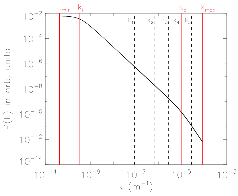
Figure 1: $P(k)$ in arbitrary units as a function of $k$ with the energy, inertial, and dissipation ranges. The wavenumber $k_{min}$, $k_{i}$, $k_{b}$, and $k_{max}$ are indicated in red lines, and wavenumber $k_{1}$, $k_{2}$, $k_{3}$, $k_{4}$, and $k_{5}$ are indicated in dashed lines.

In addition, we describe some important parameters relevant to the numerical simulation box. For the spatial domain size in $x$, $y$, and $z$ directions, we take $x_{\text{box}}=y_{\text{box}}=z_{\text{box}}=10^{4}\lambda$, which defines a box large enough so that electrons are not easy to escape. The power spectrum of turbulence is continuous and nonperiodic in nature, so there is no way to realize the actual turbulence in the simulations. We here adopt a turbulence box of size $L_{x}=L_{y}=10\lambda$, and $L_{z}=50\lambda$, for the 2D and slab components, respectively. In fact, we have checked that it is very difficult for electrons to transport in space larger than the size of the slab-2D box. The number of grids in the slab modes is set as $N_{z}=2^{22}$, and the minimum and maximum wavenumber of the slab turbulence are $k_{min}=2\pi/L_{z}\sim 4.2\times 10^{-11}$ m^-1 and $k_{max}=2\pi N_{z}/2L_{z}\sim 8.8\times 10^{-5}$ m^-1, respectively. We plot the $P(k)$ in arbitrary units as a function of $k$ in Figure 1, with the wavenumber $k_{min}$, $k_{i}$, $k_{b}$, and $k_{max}$ indicated in red vertical lines. We also show the minimum resonant wavenumber $k_{1}$, $k_{2}$, $k_{3}$, $k_{4}$, and $k_{5}$ indicated in dashed lines for electrons with energies of $10,000$, $1,000$, $100$, $10$, and $1$ keV, respectively. It can be clearly seen that low-energy electrons which are below 10 keV resonate in the dissipation range, while the electrons with energies above 10 keV may resonate in the inertial range. For the 2D modes, we set the number of grids as $N_{x}=N_{y}=4096$. Note that we take smaller box size in perpendicular direction than that in parallel direction since the movement range of particles in perpendicular directions is much smaller than that in parallel direction because of the smaller perpendicular diffusion coefficients. For more details on the settings and realization of the slab-2D magnetic field model in numerical code, see Qin et al. (2002a, b), Qin (2002), Zhang et al. (2017), and Kong et al. (2017).

A large number of electrons with energies of 1 keV in the upstream plasma frame at $z_{0}=-5.80\times 10^{-5}$ AU are isotropically injected, and each electron’s trajectory is obtained by solving the Lorentz motion equation in the shock frame of reference with a fourth-order Runge–Kutta method with an adjustable time step which maintains accuracy of the order of $10^{-9}$. The motion equation is given by

$$\frac{\mathrm{d}\bm{p}}{\mathrm{d}t}=q\left[\bm{E}(\bm{r},t)+\bm{v}\times\bm{B}(\bm{r},t)\right],$$ (4)

where $\bm{p}$ is the particle momentum, $\bm{v}$ is the particle velocity, $q$ is the electron charge, t is time, and the frame of reference is moving with the shock front. $\bm{E}=-\bm{U}\times\bm{B}$ is the convective electric field under the MHD approximation.

3 Numerical RESULTS

3.1 Effects of shock geometry and turbulence level

Using numerical simulations, we first investigate the acceleration of electrons at shocks with different angles $\theta_{\text{Bn}}$ between the shock normal and the upstream mean magnetic field, and different levels of magnetic turbulence $\left(b/B_{0}\right)^{2}$. We change $\theta_{\text{Bn}}$ from 0^∘ to 90^∘ with 15^∘ interval. For each value of $\theta_{\text{Bn}}$, $\left(b/B_{0}\right)^{2}$ varies in four values, $0.01$, $0.1$, $1.0$, and $10.0$. In each simulation with certain values of $\theta_{\text{Bn}}$ and $\left(b/B_{0}\right)^{2}$, we calculate the trajectories of electrons for $t_{\text{acc}}=23.2$ min, which is equivalent to the value of the acceleration time in Guo & Giacalone (2015), and at the end of simulations the kinetic energy is computed in the reference frame of shock front.

Figure 2 shows the energy spectra of electrons downstream of the shock at the end of simulations for different shock normal angles $\theta_{\text{Bn}}$ and turbulence levels $\left(b/B_{0}\right)^{2}$. Dashed and solid lines indicate $\theta_{\text{Bn}}=0^{\circ}$ and $90^{\circ}$, respectively. Black, yellow, blue, and red lines are for $\left(b/B_{0}\right)^{2}=0.01$, $0.1$, $1.0$, and $10.0$, respectively. For the cases of parallel shocks (dashed lines) we have following results. It is shown that with low turbulence levels, $\left(b/B_{0}\right)^{2}=0.01$ and $0.1$, the energy spectrum curves of black and yellow dashed lines, respectively, abruptly decrease with the increase of electron energy in the range around 1–10 keV. However, with $\left(b/B_{0}\right)^{2}=0.1$, the energy spectrum curve has higher level in the energy range around 1–10 keV, and it becomes flat in the higher energy range around 10–200 keV, and then decreases again in the even higher energy range around 200–600 keV. The energy spectrum with higher turbulence level, $\left(b/B_{0}\right)^{2}=1.0$, indicated by blue dashed line is larger than the one with $\left(b/B_{0}\right)^{2}=0.1$, and the spectral index in the range around 1–200 keV is also larger, and the energy of particles extends as high as $1$ MeV. When the turbulence level increases to $\left(b/B_{0}\right)^{2}=10.0$ (red dashed line), the energy spectrum becomes even larger, and electrons are found to be accelerated to the energies as high as $2$ MeV. On the other hand, for perpendicular shocks ($\theta_{\text{Bn}}=90^{\circ}$), all of the spectra curves of the accelerated particles downstream of the shocks for $\left(b/B_{0}\right)^{2}=0.01$, $0.1$, $1.0$ and $10.0$ indicated by black, yellow, blue, and red solid lines, respectively, are similar in the energy range around 1–10 keV, but in the energy range $\gtrsim 10$ keV, the ones with $\left(b/B_{0}\right)^{2}=0.01$ and $0.1$ are larger than that with $\left(b/B_{0}\right)^{2}=1$ and $10$, and in the range $\gtrsim 100$ keV, the one with $\left(b/B_{0}\right)^{2}=0.01$ is much larger than the one with $\left(b/B_{0}\right)^{2}=0.1$. In addition, the spectrum for parallel shock (parallel spectrum hereafter) with $\left(b/B_{0}\right)^{2}=10$ is similar as the spectra for perpendicular shocks (perpendicular spectra hereafter) in the energy range around 1–10 keV. Furthermore, the perpendicular one with $\left(b/B_{0}\right)^{2}=0.01$ is larger than the parallel one with $\left(b/B_{0}\right)^{2}=10$ in the energy range $\gtrsim 10$ keV, but the perpendicular one with $\left(b/B_{0}\right)^{2}=0.1$ is smaller than the parallel one with $\left(b/B_{0}\right)^{2}=10$ in the energy range $\gtrsim 200$ keV, and the perpendicular ones with $\left(b/B_{0}\right)^{2}=1$ and $10$ are smaller than the parallel ones with $\left(b/B_{0}\right)^{2}=1$ and $10$ in the energy range $\gtrsim 100$ keV.

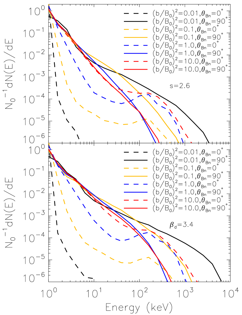
Figure 3: Top and bottom panels are similar as Figure 2, except that $s=2.6$ and $\beta_{d}=3.4$, respectively.

In this work we generally do not vary compression ratio $s$ for simplicity, and we consider strong shock acceleration, so we set $s=4$. For comparison, we also make simulations with $s=2.6$. Moreover, because spacecraft observations of the spectral index in the dissipation range vary in the range $-4<\beta_{d}<-1$ (e.g., Smith et al., 2006), we perform additional simulations with a spectral index value $\beta_{d}=3.4$ for comparison. Top and bottom panels of Figure 3 show simulation results for cases similar as that in Figure 2 except that $s=2.6$ and $\beta_{d}=3.4$, respectively. In both panels of Figure 3, the spectral features for various values of the turbulence level at parallel and perpendicular shocks, in general, are similar to those shown in Figure 2. For instance, in the energy range of 1–10 keV, the spectra for perpendicular shocks and that for parallel shocks with $(b/B_{0})^{2}=10.0$ are similar, with values higher than that for parallel shocks with $(b/B_{0})^{2}=0.01$, $0.1$, and $1.0$. In addition, the perpendicular shocks for low turbulence levels ($(b/B_{0})^{2}=0.01$ and $0.1$) accelerate electrons to higher energies compared to that for high turbulence levels ($(b/B_{0})^{2}=1.0$ and $10.0$). The details of the energy spectra in Figure 3, however, are different from that shown in Figure 2. For example, for weak shocks with $s=2.6$ in the top panel, in any condition of turbulence level and $\theta_{\text{Bn}}$, the spectra extend to lower energies in comparison with the strong shocks with $s=4.0$ shown in Figure 2. In addition, in the energy range about 10–200 keV, for the case of steeper spectral slope in the turbulence dissipation range ($\beta_{d}=3.4$) in the bottom panel of Figure 3, the spectrum for $(b/B_{0})^{2}=0.1$ at parallel shock is less flatter compared to the similar case but $\beta_{d}=2.7$ in Figure 2. Figure 3 suggests that $s=4$ and $\beta_{d}=2.7$ can be used as representative parameters to study shock acceleration. Therefore, in the rest of the paper, we study electron acceleration at shocks in fixed compression ratio, $s=4$, and spectral index in dissipation range $\beta_{d}=2.7$.

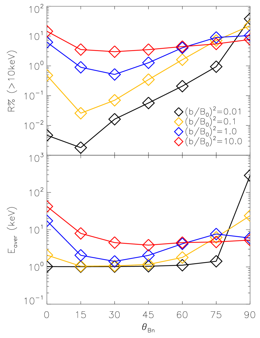
Figure 4: The acceleration efficiency of electrons versus shock-normal angle for various turbulence levels. $R\%$ (top panel) and $E_{\text{aver}}$ (bottom panel) represents the fraction of accelerated electrons with energies of more than 10 keV and average energy of electrons, respectively, at the end of the simulations.

In Figure 4 as a function of shock normal angle $\theta_{\text{Bn}}$, we present the percentage $R\%$ of electrons accelerated to more than 10 keV (top panel) and average electron energy $E_{\text{aver}}$ (bottom panel) at the end of simulations, for four different turbulence levels $\left(b/B_{0}\right)^{2}=0.01$, $0.1$, $1.0$, and $10$ indicated by black, yellow, blue, and red lines, respectively. Here, we use $R\%$ and $E_{\text{aver}}$ as measures of the efficiency of electron acceleration. It can be seen that the accelerated percentage, $R\%$, and average energy $E_{\text{aver}}$ have the same trend as a function of $\theta_{\text{Bn}}$, i.e., they decrease with $\theta_{\text{Bn}}$ increasing from $0^{\circ}$ to $15^{\circ}$, and then generally increase with $\theta_{\text{Bn}}$ increasing from $30^{\circ}$ to $90^{\circ}$. In addition, with $\theta_{\text{Bn}}\lesssim 60^{\circ}$ ($\theta_{\text{Bn}}>75^{\circ}$), $R\%$ and $E_{\text{aver}}$ increase (decrease) with the increasing of turbulence level. It is shown that, in parallel shocks with $\theta_{\text{Bn}}\sim 0^{\circ}$, $R\%$ and $E_{\text{aver}}$ are much larger with high turbulence level than that with low turbulence level, on the other hand, in perpendicular shocks with $\theta_{\text{Bn}}\sim 90^{\circ}$, $R\%$ and $E_{\text{aver}}$ are much larger with low turbulence level than that with high turbulence level. Furthermore, as $\theta_{\text{Bn}}\gtrsim 30^{\circ}$ the acceleration efficiency in general increases with increasing of $\theta_{\text{Bn}}$, and its largest variation with $\theta_{\text{Bn}}$ is seen at a low turbulence level $\left(b/B_{0}\right)^{2}=0.01$. $R\%$ and $E_{\text{aver}}$ in the case of perpendicular shock and $\left(b/B_{0}\right)^{2}=0.01$ are larger than that in the case of parallel shock and $\left(b/B_{0}\right)^{2}=10$. We can also see that in high turbulence level, the shock acceleration efficiency of electrons is in weak dependence of shock normal angle, especially when $\theta_{\text{Bn}}>0^{\circ}$.

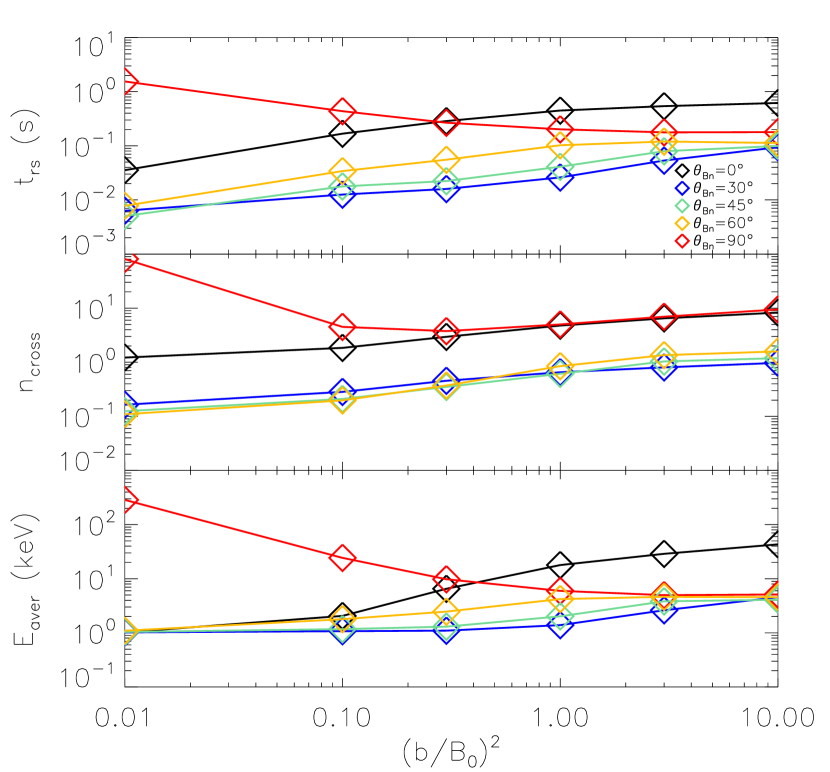
Figure 5: Average time particles staying within a gyration radius from the shock front $t_{\text{rs}}$, average shock crossing times $n_{\text{cross}}$, and average energy $E_{\text{aver}}$, in top, middle, and bottom panels, respectively, as a function of turbulence level. Black, blue, green, yellow, and red lines indicate $\theta_{\text{Bn}}=0^{\circ}$, $30^{\circ}$, $45^{\circ}$, $60^{\circ}$, $90^{\circ}$, respectively.

In Figure 5 we continue to study shock acceleration of electrons. Black, blue, green, yellow, and red lines indicate $\theta_{\text{Bn}}=0^{\circ}$, $30^{\circ}$, $45^{\circ}$, $60^{\circ}$, and $90^{\circ}$, respectively. The top panel shows average time particles staying within a gyration radius from the shock front $t_{\text{rs}}$ as a function of turbulence level $\left(b/B_{0}\right)^{2}$. From this panel it is shown that with low turbulence level, $\left(b/B_{0}\right)^{2}=0.01$, particles would stay within a gyration radius from the shock front for a long and short time in the cases of perpendicular and parallel shocks, respectively. In addition, for oblique shocks, i.e., $\theta_{\text{Bn}}=30^{\circ}$, $45^{\circ}$, and $60^{\circ}$, $t_{\text{rs}}$ is much smaller than that for both parallel and perpendicular shocks. As $\left(b/B_{0}\right)^{2}$ increases from $0.01$ to $10$, $t_{\text{rs}}$ for perpendicular shocks is decreasing while $t_{\text{rs}}$ for parallel and oblique shocks is increasing. With $\left(b/B_{0}\right)^{2}\sim 0.3$, $t_{\text{rs}}$ for perpendicular and parallel shocks are equal, and with $\left(b/B_{0}\right)^{2}\gg 0.3$, $t_{\text{rs}}$ for parallel shocks is larger than that for perpendicular ones. However, $t_{\text{rs}}$ for perpendicular shocks with $\left(b/B_{0}\right)^{2}=0.01$ is much larger than that for parallel ones, and $t_{\text{rs}}$ for oblique shocks is always smaller than that for perpendicular and parallel ones. The middle panel shows average crossing times $n_{\text{cross}}$ as a function of $\left(b/B_{0}\right)^{2}$. From this panel it is shown that for parallel shocks particles would cross the shock front more times with the increasing of $\left(b/B_{0}\right)^{2}$. However, for perpendicular shock acceleration, $n_{\text{cross}}$ would decrease as $\left(b/B_{0}\right)^{2}$ increases from $0.01$ to $\sim 0.3$, and it would have the similar value as that for parallel shocks with $\left(b/B_{0}\right)^{2}\gtrsim 0.3$. In addition, for oblique shocks, $n_{\text{cross}}$ has the similar trend as that for parallel shocks but in a much lower level. Bottom panel shows average energy of particles at the end of simulations $E_{\text{aver}}$ as a function of turbulence level. From this panel it is shown that as $\left(b/B_{0}\right)^{2}$ is very small, i.e., $\left(b/B_{0}\right)^{2}=0.01$, $E_{\text{aver}}\gg E_{0}$ for perpendicular shocks, but $E_{\text{aver}}\sim E_{0}$ for parallel and oblique shocks. As $\left(b/B_{0}\right)^{2}$ increases from $0.01$ to $10$, $E_{\text{aver}}$ decreases and increases for perpendicular and non-perpendicular shocks, respectively. However, $E_{\text{aver}}$ for parallel shocks would increases more sharply than that for oblique shocks with $\left(b/B_{0}\right)^{2}$ in the range from $0.1$ to $10$, so $E_{\text{aver}}$ for parallel shocks is much larger than that for oblique shocks with $\left(b/B_{0}\right)^{2}\gtrsim 0.1$. With $\left(b/B_{0}\right)^{2}\lesssim 0.4$ and $\gtrsim 0.4$, $E_{\text{aver}}$ for perpendicular shocks is larger and smaller than that for parallel ones, respectively.

From Figure 5 we can see that as turbulence level is very low, for perpendicular shocks particles could stay near the shock front for a long time, so they can get large acceleration from SDA, and for parallel shocks particles could not get efficient parallel scatterings to cross the shock front for many times to get large acceleration from first-order Fermi scattering process. As $\left(b/B_{0}\right)^{2}$ increases, for perpendicular shocks, the local magnetic fields would have larger component across the shock front so that it is more difficult for particles to keep near the shock front to get acceleration from SDA, but for parallel shocks, particles would get stronger parallel scatterings to cross the shock front many times and get acceleration from first-order Fermi process. In addition, for parallel shocks with large $\left(b/B_{0}\right)^{2}$, there is strong local magnetic field component perpendicular to the shock normal direction, so particles could also get acceleration from SDA. Furthermore, for oblique shocks, following results could be obtained: Firstly, particles can not stay near the shock front for long time to get large acceleration from SDA since there is strong cross shock magnetic component. Secondly, as $\left(b/B_{0}\right)^{2}$ is large, the parallel scatterings of particles only have partial contribution to shock front crossing because of the field obliquity, so that particles can not get large acceleration from first-order Fermi process too. Therefore, oblique shocks have low acceleration effects for both low and high turbulence levels.

3.2 Effects of shock thickness

We next examine the effect of shock thickness on electron acceleration by perpendicular shocks with $\left(b/B_{0}\right)^{2}=0.1$ and $1$, by varying $L_{\text{diff}}$ in Equation (1).

Figure 6 shows the average energy (top panel) and average gyro-radii considering pitch angle and upstream background magnetic field (bottom panel) versus shock thickness $L_{\text{diff}}$ for $\theta_{\text{Bn}}=90^{\circ}$ and $\left(b/B_{0}\right)^{2}=0.1$. At the end of simulations with $t_{\text{acc}}=23.2$ min, we calculate average energy and gyro-radii of particles with significant acceleration, i.e., for particles from top, second, third, fifth, and seventh $2\%$ of accelerated electrons ordered in energy with solid, dotted, dashed, dash-dotted, and dash-dotted-dotted lines, respectively. The blue dotted vertical lines (from left to right) indicate the $L_{\text{diff}}$ as the maximum gyro-radii of $10$ keV ($r_{10\text{keV}}\sim 1.13\times 10^{5}$ m), $100$ keV ($r_{100\text{keV}}\sim 3.72\times 10^{5}$ m), and $1000$ keV ($r_{1000\text{keV}}\sim 1.58\times 10^{6}$ m) electrons in the upstream. In the bottom panel, the red solid line indicates $R_{\text{gyro}}=L_{\text{diff}}$. It is shown that there exists a bend-over thickness $L_{\text{diff,b}}$, the average energy does not have obvious variation for thin shock thickness $L_{\text{diff}}\lesssim L_{\text{diff,b}}$, while it decreases rapidly with the increasing of $L_{\text{diff}}$ when $L_{\text{diff}}\gtrsim L_{\text{diff,b}}$. It is seen that $L_{\text{diff,b}}$ is in the scale of the average gyro-radii of particles.

For each curve of $R_{\text{gyro}}$ as function of $L_{\text{diff}}$ of the top, second, third, …, twelfth $2\%$ of accelerated particles ordered in energy, we fit the four data points of the smallest $L_{\text{diff}}$ as a line in log-log space, and fit the five data points of the largest $L_{\text{diff}}$ as another line in log-log space. The intersection of the two lines are assumed to be the bend-over point, denoted as $(L_{\text{diff,b}},R_{\text{gyro,b}})$. Figure 7 shows $R_{\text{gyro,b}}$ as a function of $L_{\text{diff,b}}$ from the fitting, with the red line indicating $R_{\text{gyro,b}}=L_{\text{diff,b}}$. It is shown that generally the bend-over points of the curves, $E_{\text{aver}}$–$L_{\text{diff}}$, can be approximately expressed as $R_{\text{gyro,b}}=L_{\text{diff,b}}$.

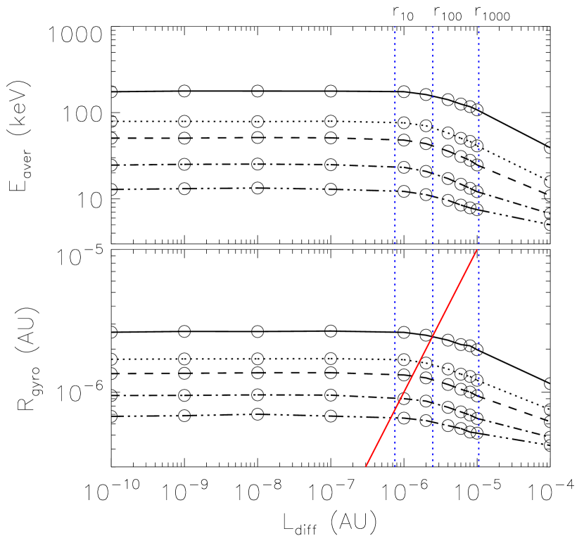
Figure 8: Similar to Figure 6 except that the turbulence level is $\left(b/B_{0}\right)^{2}=1.0$.

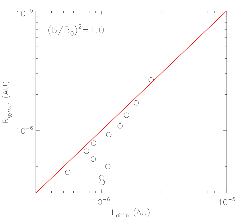
Figure 9: Similar as Figure 7 except that $\left(b/B_{0}\right)^{2}=1.0$.

Similar phenomenon can also be shown in the case of $\theta_{\text{Bn}}=90^{\circ}$ with higher turbulence level. Figures 8 and 9 are similar as Figures 6 and 7, respectively, except that $\left(b/B_{0}\right)^{2}=1.0$. Figures 6–9 suggest that there exists a critical length scale of shock thickness for perpendicular shocks in the scale of the average gyro-radii of particles with different magnetic turbulence levels $\left(b/B_{0}\right)^{2}$, the only difference is that with higher $\left(b/B_{0}\right)^{2}$ particles get weaker acceleration.

4 CONCLUSIONS AND discussion

In this paper, we use test particle simulations that include pre-existing two-component magnetic field turbulence (Qin et al., 2002a, b; Qin, 2002) upstream and downstream of the shock (Kong et al., 2017) to study electron acceleration. In our numerical model, we generate magnetic turbulence of slab component with the dissipation range in which low-energy electrons resonate, since electrons have higher gyrofrequency because of their light mass. We investigate the effects of the turbulence level $\left(b/B_{0}\right)^{2}$ and shock obliquity $\theta_{\text{Bn}}$ on the accelerated electrons spectra. It is shown that at perpendicular shocks the acceleration of electrons, which depends mainly on SDA, is found enhanced under lower turbulence levels, since it is suggested that in the presence of turbulence, the drift coefficients are reduced (e.g., Engelbrecht et al., 2017). In addition, at parallel shocks the acceleration of electrons is enhanced under higher turbulence levels with the mechanism as the following. On the one hand, it is assumed that parallel shocks can strongly accelerate particles with first-order Fermi mechanism if the turbulence level is high since there would exist effective particle scatterings to cause multiple shock crossings. On the other hand, with parallel shocks, particles do not feel drift effects due to the large scale background magnetic field, so there is no acceleration from SDA in weak turbulence. However, with stronger turbulence, there exists large local component of magnetic field perpendicular to the shock normal affected by magnetic turbulence, due to which particles would feel drift effects, therefore, electrons could get large acceleration from SDA. Moreover, for oblique shocks the acceleration of electrons is weak with both low and high turbulence levels. Our results also show that parallel shock acceleration with large turbulence level (the highest parallel shock acceleration) is less effective than perpendicular shock acceleration with small turbulence (the highest perpendicular shock acceleration). The reason might be that SDA is more effective than first-order Fermi acceleration, and in a perpendicular shock with low turbulence level, the shock acceleration is mainly from SDA, but in a parallel shock with high turbulence level, only part of shock acceleration is from SDA. Recently, Yang et al. (2018) studied acceleration of electrons by ICME-driven shocks by comparing strongest parallel and perpendicular shock acceleration events observed by the WIND 3DP instrument from 1995 through 2014 at 1 AU. They found that quasi-perpendicular shocks are more effective in the acceleration of electrons than quasi-parallel shocks are. It is shown that our results are compatible to the observations (Yang et al., 2018). The acceleration efficiency in general increases with the increasing of $\theta_{\text{Bn}}$, and its largest variation with $\theta_{\text{Bn}}$ is seen at a low turbulence level $\left(b/B_{0}\right)^{2}=0.01$. When strong magnetic fluctuations, i.e., $\left(b/B_{0}\right)^{2}=10.0$, exists at the shock front, electron acceleration is found weakly dependent on the shock-normal angle, which is in agreement with the study by Guo & Giacalone (2015). However, although Guo & Giacalone (2015) showed that perpendicular shocks with $\left(b/B_{0}\right)^{2}=1$ are more effective to accelerate particles than that with $\left(b/B_{0}\right)^{2}=10$, perpendicular shocks with low turbulence level, i.e., $\left(b/B_{0}\right)^{2}=0.1$ are less effective to accelerate particles than that with high turbulence, i.e., $\left(b/B_{0}\right)^{2}=1$ and $10.0$. We think the difference is because of the difference in the turbulence models we adopt.

Furthermore, we study the impact of shock thickness on the electron acceleration at perpendicular shocks. For the dependence of electron acceleration on the shock thickness, our simulations with perpendicular shocks indicate that there exists a bend-over thickness $L_{\text{diff,b}}$ in the scale of particles gyro-radii. The acceleration efficiency does not change evidently if the shock thickness is much smaller than $L_{\text{diff,b}}$. However, if the shock thickness is much larger than $L_{\text{diff,b}}$, the acceleration efficiency starts to drop abruptly. Previous studies have shown that the shock thickness may be of the order of ion inertial length ($c/\omega_{pi}$) (Russell et al., 1982; Newbury et al., 1998), electron inertial length ($c/\omega_{pe}$) (Newbury & Russell, 1996; Yang et al., 2013), or convected ion gyroradius ($U_{1}/\Omega_{ci,2}$) (Bale et al., 2003). Different length scale of shock thickness in solar wind would have different shock acceleration efficiency. In the condition of this work, our simulations show that the bend-over thickness $L_{\text{diff,b}}$ is in the order of ion inertial length, however, in other conditions, the bend-over thickness may be in other length scale.

In this work, we mainly concentrate on strong shock ($s=4$) acceleration of electrons. In the future, we may study the weak strength ($s=2.6$) shock acceleration in detail, so we are able to investigate what would happen in the termination shock. In addition, the pickup ion formation-driven waves which would add an extra component to the slab component of magnetic turbulence spectrum, essentially changing its form and level at wavenumbers corresponding to the proton gyrofrequency (see, e.g., Williams & Zank, 1994), could have a significant effect on low-energy electron transport parameters in the outer heliosphere (e.g., Engelbrecht, 2017). However, because of our model limitations, we do not consider the pickup ion formation-driven waves in turbulence. Furthermore, in our turbulence model, we mainly consider gentle spectral index ($\beta_{d}=-2.7$) in the dissipation range. Moreover, we do not include dissipation range in 2D component. We also do not include the variation of ratio of slab/2D magnetic turbulence energy in dissipation range. In the future, we may modify our model to make turbulence more realistic, e.g., we may include the pickup ion formation-driven waves in our model. We could also consider to include 2D dissipation range in magnetic turbulence. In addition, in dissipation range, we may vary the turbulence spectra index and the ratio of slab/2D magnetic turbulence energy.

Prinsloo et al. (2017) used modulation model to study GCR electrons and suggested that DSA can explain observed increases in electron intensities at the termination shock with ad hoc models for the transport parameters. It is interesting to find out whether the approach taken in the numerical simulations in this paper would agree with the conclusions of Prinsloo et al. (2017) if the model is set up for termination shock conditions in the future.

Figure 2: Simulated downstream energy spectra at $t_{\text{acc}}=23.2$ min for different shock-normal angles $\theta_{\text{Bn}}$ and turbulence levels $\left(b/B_{0}\right)^{2}$. Dashed and solid lines indicate $\theta_{\text{Bn}}=0^{\circ}$ and $\theta_{\text{Bn}}=90^{\circ}$, respectively. Black, yellow, blue, and red lines are for $\left(b/B_{0}\right)^{2}=0.01$, 0.1, 1.0, and 10.0, respectively. The kinetic energy of electrons is measured in the shock frame.

Figure 6: Average energy (upper panel) and average gyro-radii considering pitch angle and upstream background magnetic field (bottom panel) versus shock thickness $L_{\text{diff}}$ for $\theta_{\text{Bn}}=90^{\circ}$ and $\left(b/B_{0}\right)^{2}=0.1$. Solid, dotted, dashed, dash-dotted, and dash-dotted-dotted lines indicate particles from top, second, third, fifth, and seventh $2\%$ of accelerated electrons ordered in energy. The dotted vertical lines in each panel indicate the $L_{\text{diff}}$ equals to the gyro-radii of 10, 100 and 1000 keV electrons. Red line indicates $R_{\text{gyro}}=L_{\text{diff}}$.

Figure 7: $R_{\text{gyro,b}}$ as a function of $L_{\text{diff,b}}$ with $\left(b/B_{0}\right)^{2}=0.1$. Solid line indicates $R_{\text{gyro,b}}=L_{\text{diff,b}}$.

Table 1: Input Parameters for Simulations

Parameter		Value
$U_{1}$		500 km s-1
$s$		4
$B_{01}$		3 nT
$M_{\text{A1}}$		10
$L_{\text{diff}}$		9.28$\times 10^{-6}$ AU
$\lambda$		0.02 AU
$\theta_{1}$		0∘, 15∘, 30∘, 45∘, 60∘, 75∘, 90∘
$\left(b/B_{0}\right)^{2}$		0.01, 0.1, 1.0, 10.0
$z_{0}$		-5.80$\times 10^{-5}$ AU
$E_{0}$		1 keV
$t_{acc}$		23.2 min

References

- Axford et al. (1977) Axford, W. I., Leer, E., & Skadron, G. 1977, Proc. 15th ICRC, 11, 132
- Bale et al. (2003) Bale, S. D., Mozer, F. S., & Horbury, T. S. 2003, PhRvL, 91, 265004
- Bell (1978) Bell, A. R. 1978, MNRAS, 182, 147
- Bieber et al. (1996) Bieber, J. W., Wanner, W., & Matthaeus, W. H. 1996, J. Geophys. Res., 101, 2511
- Bieber et al. (2004) Bieber, J. W., Matthaeus, W. H., Shalchi, A. & Qin, G. 2004, Geophys. Res. Lett., 31, L10805
- Blandford & Ostriker (1978) Blandford, R. D., & Ostriker, J. P. 1978, ApJ, 221, L29
- Chen et al. (2010) Chen, C. H. K., Horbury, T. S., & Schekochihin, A. A., et al. 2010, Phys. Rev. Lett., 104, 255002
- Classen & Aurass (2002) Classen, H. T. & Aurass, H. 2002, A&A, 384, 1098
- Decker & Vlahos (1986a) Decker, R. B., & Vlahos, L. 1986a, ApJ, 306, 710
- Decker & Vlahos (1986b) Decker, R. B., & Vlahos, L. 1986b, J. Geophys. Res., 91, 13349
- Desai & Burgess (2008) Desai, M. I., & Burgess, D. 2008, J. Geophys. Res., 113, A00B06
- Dosch et al. (2013) Dosch, A., Adhikari, L., & Zank, G. P. 2013, 13th International Solar Wind Conference (Solar Wind 13), 1539, 155
- Engelbrecht (2017) Engelbrecht, N. E. 2017, ApJ, 849, L15
- Engelbrecht et al. (2017) Engelbrecht, N. E., Strauss, R. D., le Roux, J. A., & Burger, R. A. 2017, ApJ, 841, 107
- Ellison & Ramaty (1985) Ellison, D. C., & Ramaty, R. 1985, ApJ, 298, 400
- Eraker (1982) Eraker, J. H. 1982, ApJ, 257, 862
- Fermi (1949) Fermi, E. 1949, Phys. Rev. 75, 1169
- Florinski (2009) Florinski, V. 2009, Space Sci. Rev., 143, 111
- Forman & Webb (1985) Forman, M. A., & Webb, G. M. 1985, in Collisionless Shocks in the Heliosphere: A Tutorial Review, Geophysical Monograph, Vol. 34, ed. R. G. Stone & B. T. Tsurutani (Washington, DC: American Geophysical Union), 91
- Giacalone (2005) Giacalone, J. 2005, ApJ, 624, 765
- Giacalone & Jokipii (2009) Giacalone, J., & Jokipii, J. R. 2009, ApJ, 701, 1865
- Guo & Giacalone (2015) Guo, F., & Giacalone, J. 2015, ApJ, 802, 97
- Gray et al. (1996) Gray, P. C., Pontius, D. H., Jr., & Matthaeus, W. H. 1996, Geophys. Res. Lett., 23, 965
- Guo et al. (2014) Guo, X. Y., Sironi, L., & Narayan, R. 2014, ApJ, 794, 153
- Holman & Pesses (1983) Holman, G. D., & Pesses, M. E. 1983, ApJ, 267, 837
- Howes et al. (2008) Howes, G. G., Cowley, S. C., & Dorland, W., et al. 2008, J. Geophys. Res., 113, A05103
- Jokipii (1982) Jokipii, J. R. 1982, ApJ, 255, 716
- Klassen et al. (2002) Klassen, A., Bothmer, V., & Mann, G., et al. 2002, A&A, 385, 1078
- Kong et al. (2017) Kong, F.-J., Qin, G., & Zhang, L.-H. 2017, ApJ, 845, 43
- Krymsky (1977) Krymsky, G. F. 1977, Dokl. Akad. Nauk SSSR, 234, 1306
- Lara et al. (2003) Lara, A., Gopalswamy, N., Nunes, S., Muoz, G., & Yashiro, S. 2003, Geophys. Res. Lett., 30, 8016
- le Roux & Webb (2009) le Roux, J. A., & Webb, G. M. 2009, ApJ, 693, 534
- Leamon et al. (1999) Leamon, R. J., Smith, C. W., Ness, N. F., & Wong, H. K. 1999, J. Geophys. Res., 104, 22331
- Lee et al. (1996) Lee, M. A., Shapiro, V. D., & Sagdeev, R. Z. 1996, J. Geophys. Res., 101, 4777
- Li et al. (2013) Li, G., Kong, X., Zank, G., & Chen, Y. 2013, ApJ, 769, 22
- Mann et al. (2001) Mann, G., Classen, H. T., & Motschmann, U. 2001, J. Geophys. Res., 106, 25323
- Matthaeus et al. (1990) Matthaeus, W. H., Goldstein, M. L., & Roberts, D. A. 1990, J. Geophys. Res., 95, 20673
- Miller et al. (1996) Miller, J. A., LaRosa, T. N., & Moore, R. L. 1996, ApJ, 461, 445
- Matthaeus et al. (2003) Matthaeus, W. H., Qin, G., Bieber, J. W., & Zank, G. P. 2003, ApJ, 590, L53
- Moses (1987) Moses, D. 1987, ApJ, 313, 471
- Neergaard Parker & Zank (2012) Neergaard Parker, L., & Zank, G. P. 2012, ApJ, 757, 97
- Neergaard Parker et al. (2014) Neergaard Parker, L., Zank, G. P., & Hu, Q. 2014, ApJ, 782, 52
- Newbury & Russell (1996) Newbury, J. A., & Russell, C. T. 1996, Geophys. Res. Lett., 23, 781
- Newbury et al. (1998) Newbury, J. A., Russell, C. T., & Gedalin, M. 1998, J. Geophys. Res., 103, 29581
- Osman & Horbury (2007) Osman, K. T., & Horbury, T. S. 2007, ApJ, 654, L103
- Oughton et al. (2015) Oughton, S., Matthaeus, W. H., Wan, M., & Osman, K. T. 2015, Phil. Trans. R. Soc. A, 373, 20140152
- Prinsloo et al. (2017) Prinsloo, P. L., Potgieter, M. S., & Strauss, R. D. 2017, ApJ, 836, 100
- Qin (2002) Qin, G. 2002, PhD thesis, University of Delaware
- Qin et al. (2002a) Qin, G., Matthaeus, W. H., & Bieber, J. W. 2002a, Geophys. Res. Lett., 29, 1048
- Qin et al. (2002b) Qin, G., Matthaeus, W. H., & Bieber, J. W. 2002b, ApJ, 578, L117
- Rieger (1994) Rieger, E. 1994, Astroph. J. Suppl. Series, 90, 645
- Russell et al. (1982) Russell, C. T., Hoppe, M. M., Livesey, W. A., Gosling, J. T., & Bame, S. J. 1982, Geophys. Res. Lett., 9, 1171
- Shen & Qin (2018) Shen, Z. N., & Qin, G. 2018, ApJ, 854, 137
- Scudder et al. (1986) Scudder, J. D., Mangeney, A., & Lacombe, C., et al. 1986, J. Geophys. Res., 91, 11019
- Smith et al. (2006) Smith, C. W., Hamilton, K., Vasquez, B. J., & Leamon, R. J. 2006, ApJ, 645, L85
- Shapiro and Üçer (2003) Shapiro, V. D., & Üçer, D. 2003, Planet. Space Sci., 51, 665
- Stewart et al. (1974a) Stewart, R. T., Howard, R. A., Hansen, F., Gergely, T., & Kundu, M. 1974a, Sol. Phys., 36, 219
- Stewart et al. (1974b) Stewart, R. T., McCabe, M. K., Koomen, M. J., Hansen, R. T., & Dulk, G. A. 1974b, Sol. Phys., 36, 203
- Tsuneta & Naito (1998) Tsuneta, S., & Naito, T. 1998, ApJ, 495, L67
- Uchida et al. (1973) Uchida, Y., Altschuler, M. D., & Newkirk, G. Jr. 1973, Sol. Phys., 28, 495
- Vrsnak et al. (1995) Vrnak, B., Rudjak, V., Zlobec, P., & Aurass, H. 1995, Sol. Phys., 158, 331
- Weygand et al. (2009) Weygand, J. M., Matthaeus, W. H., Dasso, S., et al. 2009, J. Geophys. Res., 114, A07213
- Weygand et al. (2011) Weygand, J. M., Matthaeus, W. H., Dasso, S., & Kivelson, M. G. 2011, J. Geophys. Res., 116, A08102
- Williams & Zank (1994) Williams, L. L., & Zank, G. P. 1994, J. Geophys. Res., 99, 19229
- Yang et al. (2018) Yang, L., Wang, L., Li, G., et al. 2018, ApJ, 853, 89
- Yang et al. (2013) Yang, Z., Lu, Q., Gao, X., et al. 2013, PhPl, 20, 092116
- Zank & Matthaeus (1992) Zank, G. P., & Matthaeus, W. H. 1992, J. Geophys. Res., 97, 17189
- Zank et al. (2006) Zank, G. P., Li, G., Florinski, V., Hu, Q., Lario, D., & Smith, C. W. 2006, J. Geophys. Res., 111, A06108
- Zhang et al. (2017) Zhang, L.-H., Qin, G., Sun, P., & Wang, H.-N. 2017, arXiv:1702.04647