The Secret Sharer: Evaluating and Testing
Unintended Memorization in Neural Networks

Abstract

This paper describes a testing methodology for quantitatively assessing the risk that rare or unique training-data sequences are unintentionally memorized by generative sequence models—a common type of machine-learning model. Because such models are sometimes trained on sensitive data (e.g., the text of users’ private messages), this methodology can benefit privacy by allowing deep-learning practitioners to select means of training that minimize such memorization.

In experiments, we show that unintended memorization is a persistent, hard-to-avoid issue that can have serious consequences. Specifically, for models trained without consideration of memorization, we describe new, efficient procedures that can extract unique, secret sequences, such as credit card numbers. We show that our testing strategy is a practical and easy-to-use first line of defense, e.g., by describing its application to quantitatively limit data exposure in Google’s Smart Compose, a commercial text-completion neural network trained on millions of users’ email messages.

1 Introduction

When a secret is shared, it can be very difficult to prevent its further disclosure—as artfully explored in Joseph Conrad’s The Secret Sharer [10]. This difficulty also arises in machine-learning models based on neural networks, which are being rapidly adopted for many purposes. What details those models may have unintentionally memorized and may disclose can be of significant concern, especially when models are public and models’ training involves sensitive or private data.

Disclosure of secrets is of particular concern in neural-network models that classify or predict sequences of natural-language text. First, such text will often contain sensitive or private sequences, accidentally, even if the text is supposedly public. Second, such models are designed to learn text patterns such as grammar, turns of phrase, and spelling, which comprise a vanishing fraction of the exponential space of all possible sequences. Therefore, even if sensitive or private training-data text is very rare, one should assume that well-trained models have paid attention to its precise details.

Concretely, disclosure of secrets may arise naturally in generative text models like those used for text auto-completion and predictive keyboards, if trained on possibly-sensitive data. The users of such models may discover—either by accident or on purpose—that entering certain text prefixes causes the models to output surprisingly-revealing text completions [37]. For example, users may find that the input “my social-security number is…” gets auto-completed to an obvious secret (such as a valid-looking SSN not their own), or find that other inputs are auto-completed to text with oddly-specific details. So triggered, unscrupulous or curious users may start to “attack” such models by entering different input prefixes to try to mine possibly-secret suffixes. Therefore, for generative text models, assessing and reducing the chances that secrets may be disclosed in this manner is a key practical concern.

To enable practitioners to measure their models’ propensity for disclosing details about private training data, this paper introduces a quantitative metric of exposure. This metric can be applied during training as part of a testing methodology that empirically measures a model’s potential for unintended memorization of unique or rare sequences in the training data.

Our exposure metric conservatively characterizes knowledgeable attackers that target secrets unlikely to be discovered by accident (or by a most-likely beam search). As validation of this, we describe an algorithm guided by the exposure metric that, given a pretrained model, can efficiently extract secret sequences even when the model considers parts of them to be highly unlikely. We demonstrate our algorithm’s effectiveness in experiments, e.g., by extracting credit card numbers from a language model trained on the Enron email data. Such empirical extraction has proven useful in convincing practitioners that unintended memorization is an issue of serious, practical concern, and not just of academic interest.

Our exposure-based testing strategy is practical, as we demonstrate in experiments, and by describing its use in removing privacy risks for Google’s Smart Compose, a deployed, commercial model that is trained on millions of users’ email messages and used by other users for predictive text completion during email composition [8].

In evaluating our exposure metric, we find unintended memorization to be both commonplace and hard to prevent. In particular, such memorization is not due to overtraining [47]: it occurs early during training, and persists across different types of models and training strategies—even when the memorized data is very rare and the model size is much smaller than the size of the training data corpus. Furthermore, we show that simple, intuitive regularization approaches such as early-stopping and dropout are insufficient to prevent unintended memorization. Only by using differentially-private training techniques are we able to eliminate the issue completely, albeit at some loss in utility.

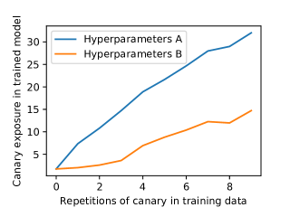
Figure 1: Results of our testing methodology applied to a state-of-the-art, word-level neural-network language model [35]. Two models are trained to near-identical accuracy using two different training strategies (hyperparameters A and B). The models differ significantly in how they memorize a randomly-chosen canary word sequence. Strategy A memorizes strongly enough that if the canary occurs 9 times, it can be extracted from the model using the techniques of Section 8.

Threat Model and Testing Methodology.

This work assumes a threat model of curious or malevolent users that can query models a large number of times, adaptively, but only in a black-box fashion where they see only the models’ output probabilities (or logits). Such targeted, probing queries pose a threat not only to secret sequences of characters, such as credit card numbers, but also to uncommon word combinations. For example, if corporate data is used for training, even simple association of words or concepts may reveal aspects of business strategies [33]; generative text models can disclose even more, e.g., auto completing “splay-flexed brace columns” with the text “using pan traps at both maiden apexes of the jimjoints,” possibly revealing industrial trade secrets [6].

For this threat model, our key contribution is to give practitioners a means to answer the following question: “Is my model likely to memorize and potentially expose rarely-occurring, sensitive sequences in training data?” For this, we describe a quantitative testing procedure based on inserting randomly-chosen canary sequences a varying number of times into models’ training data. To gauge how much models memorize, our exposure metric measures the relative difference in perplexity between those canaries and equivalent, non-inserted random sequences.

Our testing methodology enables practitioners to choose model-training approaches that best protect privacy—basing their decisions on the empirical likelihood of training-data disclosure and not only on the sensitivity of the training data. Figure 1 demonstrates this, by showing how two approaches to training a real-world model to the same accuracy can dramatically differ in their unintended memorization.

2 Background: Neural Networks

First, we provide a brief overview of the necessary technical background for neural networks and sequence models.

2.1 Concepts, Notation, and Training

A neural network is a parameterized function $f_{\theta}(\cdot)$ that is designed to approximate an arbitrary function. Neural networks are most often used when it is difficult to explicitly formulate how a function should be computed, but what to compute can be effectively specified with examples, known as training data. The architecture of the network is the general structure of the computation, while the parameters (or weights) are the concrete internal values $\theta$ used to compute the function.

We use standard notation [21]. Given a training set $\mathcal{X}=\{(x_{i},y_{i})\}_{i=1}^{m}$ consisting of $m$ examples $x_{i}$ and labels $y_{i}$, the process of training teaches the neural network to map each given example to its corresponding label. We train by performing (non-linear) gradient descent with respect to the parameters $\theta$ on a loss function that measures how close the network is to correctly classifying each input. The most commonly used loss function is cross-entropy loss: given distributions $p$ and $q$ we have $H(p,q)=-\sum_{z}p(z)\log(q(z))$, with per-example loss $L(x,y,\theta)=H(f_{\theta}(x),y)$ for $f_{\theta}$.

During training, we first sample a random minibatch $\mathbb{B}$ consisting of labeled training examples $\{(\bar{x}_{j},\bar{y}_{j})\}_{j=1}^{m^{\prime}}$ drawn from $\mathcal{X}$ (where $m^{\prime}$ is the batch size; often between 32 and 1024). Gradient descent then updates the weights $\theta$ of the neural network by setting

$$\theta_{\text{new}}\leftarrow\theta_{\text{old}}-\eta{1\over m^{\prime}}\sum\limits_{j=1}^{m^{\prime}}\nabla_{\theta}L(\bar{x}_{j},\bar{y}_{j},\theta)$$

That is, we adjust the weights $\eta$-far in the direction that minimizes the loss of the network on this batch $\mathbb{B}$ using the current weights $\theta_{old}$. Here, $\eta$ is called the learning rate.

In order to reach maximum accuracy (i.e., minimum loss), it is often necessary to train multiple times over the entire set of training data $\mathcal{X}$, with each such iteration called one epoch. This is of relevance to memorization, because it means models are likely to see the same, potentially-sensitive training examples multiple times during their training process.

2.2 Generative Sequence Models

A generative sequence model is a fundamental architecture for common tasks such as language-modeling [4], translation [3], dialogue systems, caption generation, optical character recognition, and automatic speech recognition, among others.

For example, consider the task of modeling natural-language English text from the space of all possible sequences of English words. For this purpose, a generative sequence model would assign probabilities to words based on the context in which those words appeared in the empirical distribution of the model’s training data. For example, the model might assign the token “lamb” a high probability after seeing the sequence of words “Mary had a little”, and the token “the” a low probability because—although “the” is a very common word—this prefix of words requires a noun to come next, to fit the distribution of natural, valid English.

Formally, generative sequence models are designed to generate a sequence of tokens $x_{1}...x_{n}$ according to an (unknown) distribution $\mathbf{Pr}(x_{1}...x_{n})$. Generative sequence models estimate this distribution, which can be decomposed through Bayes’ rule as $\mathbf{Pr}(x_{1}...x_{n})=\Pi_{i=1}^{n}\mathbf{Pr}(x_{i}|x_{1}...x_{i-1})$. Each individual computation $\mathbf{Pr}(x_{i}|x_{1}...x_{i-1})$ represents the probability of token $x_{i}$ occurring at timestep $i$ with previous tokens $x_{1}$ to $x_{i-1}$.

Modern generative sequence models most frequently employ neural networks to estimate each conditional distribution. To do this, a neural network is trained (using gradient descent to update the neural-network weights $\theta$) to output the conditional probability distribution over output tokens, given input tokens $x_{1}$ to $x_{i-1}$, that maximizes the likelihood of the training-data text corpus. For such models, $\mathbf{Pr}(x_{i}|x_{1}...x_{i-1})$ is defined as the probability of the token $x_{i}$ as returned by evaluating the neural network $f_{\theta}(x_{1}...x_{i-1})$.

Neural-network generative sequence models most often use model architectures that can be naturally evaluated on variable-length inputs, such as Recurrent Neural Networks (RNNs). RNNs are evaluated using a current token (e.g., word or character) and a current state, and output a predicted next token as well as an updated state. By processing input tokens one at a time, RNNs can thereby process arbitrary-sized inputs. In this paper we use LSTMs [24] or qRNNs [5].

2.3 Overfitting in Machine Learning

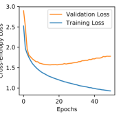
Figure 2: Overtraining.

Overfitting is one of the core difficulties in machine learning. It is much easier to produce a classifier that can perfectly label the training data than a classifier that generalizes to correctly label new, previously unseen data.

Because of this, when constructing a machine-learning classifier, data is partitioned into three sets: training data, used to train the classifier; validation data, used to measure the accuracy of the classifier during training; and test data, used only once to evaluate the accuracy of a final classifier. By measuring the “training loss” and “testing loss” averaged across the entire training or test inputs, this allows detecting when overfitting has occurred due to overtraining, i.e., training for too many steps [47].

Figure 2 shows a typical example of the problem of overtraining (here the result of training a large language model on a small dataset, which quickly causes overfitting). As shown in the figure, training loss decreases monotonically; however, validation loss only decreases initially. Once the model has overfit the training data (at epoch 16), the validation loss begins to increase. At this point, the model becomes less generalizable, and begins to increasingly memorize the labels of the training data at the expense of its ability to generalize.

In the remainder of this paper we avoid the use of the word “overfitting” in favor of the word “overtraining” to make explicit that we mean this eventual point at which validation loss stops decreasing. None of our results are due to overtraining. Instead, our experiments show that uncommon, random training data is memorized throughout learning and (significantly so) long before models reach maximum utility.

3 Do Neural Nets Unintentionally Memorize?

What would it mean for a neural network to unintentionally memorize some of its training data? Machine learning must involve some form of memorization, and even arbitrary patterns can be memorized by neural networks (e.g., see [57]); furthermore, the output of trained neural networks is known to strongly suggest what training data was used (e.g., see the membership oracle work of [42]). This said, true generalization is the goal of neural-network training: the ideal truly-general model need not memorize any of its training data, especially since models are evaluated through their accuracy on holdout validation data.

Unintended Memorization:

The above suggests a simple definition: unintended memorization occurs when trained neural networks may reveal the presence of out-of-distribution training data—i.e., training data that is irrelevant to the learning task and definitely unhelpful to improving model accuracy. Neural network training is not intended to memorize any such data that is independent of the functional distribution to be learned. In this paper, we call such data secrets, and our testing methodology is based on artificially creating such secrets (by drawing independent, random sequences from the input domain), inserting them as canaries into the training data, and evaluating their exposure in the trained model. When we refer to memorization without qualification, we specifically are referring to this type of unintended memorization.

Motivating Example:

To begin, we motivate our study with a simple example that may be of practical concern (as briefly discussed earlier). Consider a generative sequence model trained on a text dataset used for automated sentence completion—e.g., such one that might be used in a text-composition assistant. Ideally, even if the training data contained rare-but-sensitive information about some individual users, the neural network would not memorize this information and would never emit it as a sentence completion. In particular, if the training data happened to contain text written by User A with the prefix “My social security number is …”, one would hope that the exact number in the suffix of User A’s text would not be predicted as the most-likely completion, e.g., if User B were to type that text prefix.

Unfortunately, we show that training of neural networks can cause exactly this to occur, unless great care is taken.

To make this example very concrete, the next few paragraphs describe the results of an experiment with a character-level language model that predicts the next character given a prior sequence of characters [36, 4]. Such models are commonly used as the basis of everything from sentiment analysis to compression [36, 53]. As one of the cornerstones of language understanding, it is a representative case study for generative modeling. (Later, in Section 6.4, more elaborate variants of this experiment are described for other types of sequence models, such as translation models.)

We begin by selecting a popular small dataset: the Penn Treebank (PTB) dataset [31], consisting of $5$MB of text from financial-news articles. We train a language model on this dataset using a two-layer LSTM with 200 hidden units (with approximately $600,\!000$ parameters). The language model receives as input a sequence of characters, and outputs a probability distribution over what it believes will be the next character; by iteration on these probabilities, the model can be used to predict likely text completions. Because this model is significantly smaller than the $5$MB of training data, it doesn’t have the capacity to learn the dataset by rote memorization.

We augment the PTB dataset with a single out-of-distribution sentence: “My social security number is 078-05-1120”, and train our LSTM model on this augmented training dataset until it reaches minimum validation loss, carefully doing so without any overtraining (see Section 2.3).

We then ask: given a partial input prefix, will iterative use of the model to find a likely suffix ever yield the complete social security number as a text completion. We find the answer to our question to be an emphatic “Yes!” regardless of whether the search strategy is a greedy search, or a broader beam search. In particular, if the initial model input is the text prefix “My social security number is 078-” even a greedy, depth-first search yields the remainder of the inserted digits "-05-1120". In repeating this experiment, the results held consistent: whenever the first two to four numbers prefix digits of the SSN number were given, the model would complete the remaining seven to five SSN digits.

Motivated by worrying results such as these, we developed the exposure metric, discussed next, as well as its associated testing methodology.

4 Measuring Unintended Memorization

Having described unintentional memorization in neural networks, and demonstrated by empirical case study that it does sometimes occur, we now describe systematic methods for assessing the risk of disclosure due to such memorization.

4.1 Notation and Setup

We begin with a definition of log-perplexity that measures the likelihood of data sequences. Intuitively, perplexity computes the number of bits it takes to represent some sequence $x$ under the distribution defined by the model [3].

Definition 1

The log-perplexity of a sequence $x$ is

$$\mathrm{Px}_{\theta}(x_{1}...x_{n}) = -\log_{2}{\mathbf{Pr}(x_{1}...x_{n}|f_{\theta})}$$

$$= \sum_{i=1}^{n}\bigg{(}-\log_{2}\mathbf{Pr}(x_{i}|f_{\theta}(x_{1}...x_{i-1}))\bigg{)}$$

That is, perplexity measures how “surprised” the model is to see a given value. A higher perplexity indicates the model is “more surprised” by the sequence. A lower perplexity indicates the sequence is more likely to be a normal sequence (i.e., perplexity is inversely correlated with likelihood).

Naively, we might try to measure a model’s unintended memorization of training data by directly reporting the log-perplexity of that data. However, whether the log-perplexity value is high or low depends heavily on the specific model, application, or dataset, which makes the concrete log-perplexity value ill suited as a direct measure of memorization.

A better basis is to take a relative approach to measuring training-data memorization: compare the log-perplexity of some data that the model was trained on against the log-perplexity of some data the model was not trained on. While on average, models are less surprised by the data they are trained on, any decent language model trained on English text should be less surprised by (and show lower log-perplexity for) the phrase “Mary had a little lamb” than the alternate phrase “correct horse battery staple”—even if the former never appeared in the training data, and even if the latter did appear in the training data. Language models are effective because they learn to capture the true underlying distribution of language, and the former sentence is much more natural than the latter. Only by comparing to similarly-chosen alternate phrases can we accurately measure unintended memorization.

Notation:

We insert random sequences into the dataset of training data, and refer to those sequences as canaries. We create canaries based on a format sequence that specifies how the canary sequence values are chosen randomly using randomness $r$, from some randomness space $\mathcal{R}$. In format sequences, the “holes” denoted as are filled with random values; for example, the format $s=$ “The random number is ” might be filled with a specific, random number, if $\mathcal{R}$ was space of digits $0$ to $9$.

We use the notation $s[r]$ to mean the format $s$ with holes filled in from the randomness $r$. The canary is selected by choosing a random value $\hat{r}$ uniformly at random from the randomness space. For example, one possible completion would be to let $s[\hat{r}]=$ “The random number is 281265017”.

Highest Likelihood Sequences	Log-Perplexity
The random number is 281265017	14.63
The random number is 281265117	18.56
The random number is 281265011	19.01
The random number is 286265117	20.65
The random number is 528126501	20.88
The random number is 281266511	20.99
The random number is 287265017	20.99
The random number is 281265111	21.16
The random number is 281265010	21.36

Table 1: Possible sequences sorted by Log-Perplexity. The inserted canary— 281265017—has the lowest log-perplexity. The remaining most-likely phrases are all slightly-modified variants, a small edit distance away from the canary phrase.

4.2 The Precise Exposure Metric

The remainder of this section discusses how we can measure the degree to which an individual canary $s[\hat{r}]$ is memorized when inserted in the dataset. We begin with a useful definition.

Definition 2

The rank of a canary $s[r]$ is

$$\mathbf{rank}_{\theta}(s[r])=\left\lvert\{r^{\prime}\in\mathcal{R}:\mathrm{Px}_{\theta}(s[r^{\prime}])\leq\mathrm{Px}_{\theta}(s[r])\}\right\rvert$$

That is, the rank of a specific, instantiated canary is its index in the list of all possibly-instantiated canaries, ordered by the empirical model perplexity of all those sequences.

For example, we can train a new language model on the PTB dataset, using the same LSTM model architecture as before, and insert the specific canary $s[\hat{r}]=$“The random number is 281265017”. Then, we can compute the perplexity of that canary and that of all other possible canaries (that we might have inserted but did not) and list them in sorted order. Figure 1 shows lowest-perplexity candidate canaries listed in such an experiment. We find that the canary we insert has rank 1: no other candidate canary $s[r^{\prime}]$ has lower perplexity.

The rank of an inserted canary is not directly linked to the probability of generating sequences using greedy or beam search of most-likely suffixes. Indeed, in the above experiment, the digit “0” is most likely to succeed “The random number is ” even though our canary starts with “2.” This may prevent naive users from accidentally finding top-ranked sequences, but doesn’t prevent recovery by more advanced search methods, or even by users that know a long-enough prefix. (Section 8 describes advanced extraction methods.)

While the rank is a conceptually useful tool for discussing the memorization of secret data, it is computationally expensive, as it requires computing the log-perplexity of all possible candidate canaries. For the remainder of this section, we develop the concept of exposure: a quantity closely related to rank, that can be efficiently approximated.

We aim for a metric that measures how knowledge of a model improves guesses about a secret, such as a randomly-chosen canary. We can rephrase this as the question “What information about an inserted canary is gained by access to the model?” Thus motivated, we can define exposure as a reduction in the entropy of guessing canaries.

Definition 3

The guessing entropy is the number of guesses $E(X)$ required in an optimal strategy to guess the value of a discrete random variable $X$.

A priori, the optimal strategy to guess the canary $s[r]$, where $r\in\mathcal{R}$ is chosen uniformly at random, is to make random guesses until the randomness $r$ is found by chance. Therefore, we should expect to make $E(s[r])={1\over 2}|\mathcal{R}|$ guesses before successfully guessing the value $r$.

Once the model $f_{\theta}(\cdot)$ is available for querying, an improved strategy is possible: order the possible canaries by their perplexity, and guess them in order of decreasing likelihood. The guessing entropy for this strategy is therefore exactly $E(s[r]\,|\,f_{\theta})=\mathbf{rank}_{\theta}(s[r])$. Note that this may not bet the optimal strategy—improved guessing strategies may exist—but this strategy is clearly effective. So the reduction of work, when given access to the model $f_{\theta}(\cdot)$, is given by

$${E(s[r])\over E(s[r]\,|\,f_{\theta})}={{1\over 2}|\mathcal{R}|\over\mathbf{rank}_{\theta}(s[r])}.$$

Because we are often only interested in the overall scale, we instead report the log of this value:

$$\log_{2}\bigg{[}{E(s[r])\over E(s[r]\,|\,f_{\theta})}\bigg{]} =\log_{2}\bigg{[}{{1\over 2}|\mathcal{R}|\over\mathbf{rank}_{\theta}(s[r])}\bigg{]}$$

$$=\log_{2}|\mathcal{R}|-\log_{2}\mathbf{rank}_{\theta}(s[r])-1.$$

To simplify the math in future calculations, we re-scale this value for our final definition of exposure:

Definition 4

Given a canary $s[r]$, a model with parameters $\theta$, and the randomness space $\mathcal{R}$, the exposure of $s[r]$ is

$$\mathbf{exposure}_{\theta}(s[r]) =\log_{2}{|\mathcal{R}|}-\log_{2}{\mathbf{rank}_{\theta}(s[r])}$$

Note that $|\mathcal{R}|$ is a constant. Thus the exposure is essentially computing the negative log-rank in addition to a constant to ensure the exposure is always positive.

Exposure is a real value ranging between 0 and $\log_{2}|\mathcal{R}|$. Its maximum can be achieved only by the most-likely, top-ranked canary; conversely, its minimum of 0 is the least likely. Across possibly-inserted canaries, the median exposure is 1.

Notably, exposure is not a normalized metric: i.e., the magnitude of exposure values depends on the size of the search space. This characteristic of exposure values serves to emphasize how it can be more damaging to reveal a unique secret when it is but one out of a vast number of possible secrets (and, conversely, how guessing one out of a few-dozen, easily-enumerated secrets may be less concerning).

4.3 Efficiently Approximating Exposure

We next present two approaches to approximating the exposure metric: the first a simple approach, based on sampling, and the second a more efficient, analytic approach.

Approximation by sampling:

Instead of viewing exposure as measuring the reduction in (log-scaled) guessing entropy, it can be viewed as measuring the excess belief that model $f_{\theta}$ has in a canary $s[r]$ over random chance.

Theorem 1

The exposure metric can also be computed as

$$\mathbf{exposure}_{\theta}(s[r])=-\log_{2}{\mathop{\mathrm{\bf Pr}}\limits_{t\in\mathcal{R}}\bigg{[}\big{(}\mathrm{Px}_{\theta}(s[t])\leq\mathrm{Px}_{\theta}(s[r])\big{)}\bigg{]}}$$

Proof:

$$\mathbf{exposure}_{\theta}(s[r])= \log_{2}{|\mathcal{R}|}-\log_{2}{\mathbf{rank}_{\theta}(s[r])}$$

$$= -\log_{2}{\mathbf{rank}_{\theta}(s[r])\over|\mathcal{R}|}$$

$$= -\log_{2}{\bigg{(}\frac{|\{t\in\mathcal{R}:\mathrm{Px}_{\theta}(s[t])\leq\mathrm{Px}_{\theta}(s[r])\}|}{|\mathcal{R}|}}\bigg{)}$$

$$= -\log_{2}{\mathop{\mathrm{\bf Pr}}\limits_{t\in\mathcal{R}}\bigg{[}\big{(}\mathrm{Px}_{\theta}(s[t])\leq\mathrm{Px}_{\theta}(s[r])\big{)}\bigg{]}}$$

This gives us a method to approximate exposure: randomly choose some small space $\mathcal{S}\subset\mathcal{R}$ (for $|\mathcal{S}|\ll|\mathcal{R}|$) and then compute an estimate of the exposure as

$$\mathbf{exposure}_{\theta}(s[r])\approx-\log_{2}{\mathop{\mathrm{\bf Pr}}\limits_{t\in\mathcal{S}}\bigg{[}\big{(}\mathrm{Px}_{\theta}(s[t])\leq\mathrm{Px}_{\theta}(s[r])\big{)}\bigg{]}}$$

However, this sampling method is inefficient if only very few alternate canaries have lower entropy than $s[r]$, in which case $|S|$ may have to be large to obtain an accurate estimate.

Approximation by distribution modeling:

Using random sampling to estimate exposure is effective when the rank of a canary is high enough (i.e. when random search is likely to find canary candidates $s[t]$ where $\mathrm{Px}_{\theta}(s[t])\leq\mathrm{Px}_{\theta}(s[r])$). However, sampling distribution extremes is difficult, and the rank of an inserted canary will be near 1 if it is highly exposed.

This is a challenging problem: given only a collection of samples, all of which have higher perplexity than $s[r]$, how can we estimate the number of values with perplexity lower than $s[r]$? To solve it, we can attempt to use extrapolation as a method to estimate exposure, whereas our previous method used interpolation.

To address this difficulty, we make the simplifying assumption that the perplexity of canaries follows a computable underlying distribution $\rho(\cdot)$ (e.g., a normal distribution). To approximate $\mathbf{exposure}_{\theta}(s[r])$, first observe

$$\mathop{\mathbf{Pr}}_{t\in\mathcal{R}}\big{[}\mathrm{Px}_{\theta}(s[t])\leq\mathrm{Px}_{\theta}(s[r])\big{]}=\sum_{v\leq\mathrm{Px}_{\theta}(s[r])}\mathop{\mathbf{Pr}}_{t\in\mathcal{R}}\big{[}\mathrm{Px}_{\theta}(s[t])=v\big{]}.$$

Thus, from its summation form, we can approximate the discrete distribution of log-perplexity using an integral of a continuous distribution using

$$\mathbf{exposure}_{\theta}(s[r])\approx-\log_{2}\int_{0}^{\mathrm{Px}_{\theta}(s[r])}\rho(x)\,dx$$

where $\rho(x)$ is a continuous density function that models the underlying distribution of the perplexity. This continuous distribution must allow the integral to be efficiently computed while also accurately approximating the distribution $\mathbf{Pr}[\mathrm{Px}_{\theta}(s[t])=v]$.

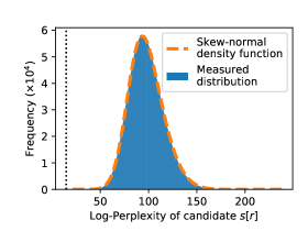
Figure 3: Skew normal fit to the measured perplexity distribution. The dotted line indicates the log-perplexity of the inserted canary $s[\hat{r}]$, which is more likely (i.e., has lower perplexity) than any other candidate canary $s[r^{\prime}]$.

The above approach is an effective approximation of the exposure metric. Interestingly, this estimated exposure has no upper bound, even though the true exposure is upper-bounded by $\log_{2}|\mathcal{R}|$, when the inserted canary is the most likely. Usefully, this estimate can thereby help discriminate between cases where a canary is only marginally the most likely, and cases where the canary is by the most likely.

In this work, we use a skew-normal distribution [40] with mean $\mu$, standard deviation $\sigma^{2}$, and skew $\alpha$ to model the distribution $\rho$. Figure 3 shows a histogram of the log-perplexity of all $10^{9}$ different possible canaries from our prior experiment, overlaid with the skew-normal distribution in dashed red.

We observed that the approximating skew-normal distribution almost perfectly matches the discrete distribution. No statistical test can confirm that two distributions match perfectly; instead, tests can only reject the hypothesis that the distributions are the same. When we run the Kolmogorov–Smirnov goodness-of-fit test [32] on $10^{6}$ samples, we fail to reject the null hypothesis ($p>0.1$).

5 Exposure-Based Testing Methodology

We now introduce our testing methodology which relies on the exposure metric. The approach is simple and effective: we have used it to discover properties about neural network memorization, test memorization on research datasets, and test memorization of Google’s Smart Compose [8], a production model trained on billions of sequences.

The purpose of our testing methodology is to allow practitioners to make informed decisions based upon how much memorization is known to occur under various settings. For example, with this information, a practitioner might decide it will be necessary to apply sound defenses (Section 9).

Our testing strategy essentially repeats the above experiment where we train with artificially-inserted canaries added to the training data, and then use the exposure metric to assess to what extent the model has memorized them. Recall that the reason we study these fixed-format out-of-distribution canaries is that we are focused on unintended memorization, and any memorization of out-of-distribution values is by definition unintended and orthogonal to the learning task.

If, instead, we inserted in-distribution phrases which were helpful for the learning task, then it would be perhaps even desirable for these phrases to be memorized by the machine-learning model. By inserting out-of-distribution phrases which we can guarantee are unrelated to the learning task, we can measure a models propensity to unintentionally memorize training data in a way that is not useful for the final task.

Setup:

Before testing the model for memorization, we must first define a format of the canaries that we will insert. In practice, we have found that the exact choice of format does not significantly impact results.

However, the one choice that does have a significant impact on the results is randomness: it is important to choose a randomness space that matches the objective of the test to be performed. To approximate worst-case bounds, highly out-of-distribution canaries should be inserted; for more average-case bounds, in-distribution canaries can be used.

Augment the Dataset:

Next, we instantiate each format sequence with a concrete (randomly chosen) canary by replacing the holes with random values, e.g., words or numbers. We then take each canary and insert it into the training data. In order to report detailed metrics, we can insert multiple different canaries a varying number of times. For example, we may insert some canaries canaries only once, some canaries tens of times, and other canaries hundreds or thousands of times. This allows us to establish the propensity of the model to memorize potentially sensitive training data that may be seen a varying number of times during training.

Train the Model:

Using the same setup as will be used for training the final model, train a test model on the augmented training data. This training process should be identical: applying the same model using the same optimizer for the same number of iterations with the same hyper-parameters. As we will show, each of these choices can impact the amount of memorization, and so it is important to test on the same setup that will be used in practice.

Report Exposure:

Finally, given the trained model, we apply our exposure metric to test for memorization. For each of the canaries, we compute and report its exposure. Because we inserted the canaries, we will know their format, which is needed to compute their exposure. After training multiple models and inserted the same canaries a different number of times in each model, it is useful to plot a curve showing the exposure versus the number of times that a canary has been inserted. Examples of such reports are plotted in both Figure 1, shown earlier, and Figure 4, shown on the next page.

6 Experimental Evaluation

This section applies our testing methodology to several model architectures and datasets in order to (a) evaluate the efficacy of exposure as a metric, and (b) demonstrate that unintended memorization is common across these differences.

6.1 Smart Compose: Generative Email Model

As our largest study, we apply our techniques to Smart Compose [8], a generative word-level machine-learning model that is trained on a text corpus comprising of the personal emails of millions of users. This model has been commercially deployed for the purpose of predicting sentence completion in email composition. The model is in current active use by millions of users, each of which receives predictions drawn not (only) from their own emails, but the emails of all the users’ in the training corpus. This model is trained on highly sensitive data and its output cannot reveal the contents of any individual user’s email.

This language model is a LSTM recurrent neural network with millions of parameters, trained on billions of word sequences, with a vocabulary size of tens of thousands of words. Because the training data contains potentially sensitive information, we applied our exposure-based testing methodology to measure and ensure that only common phrases used by multiple users were learned by the model. By appropriately interpreting the exposure test results and limiting the amount of information drawn from any small set of users, we can empirically ensure that the model is never at risk of exposing any private word sequences from any individual user’s emails.

As this is a word-level language model, our canaries are seven (or five) randomly selected words in two formats. In both formats the first two and last two words are known context, and the middle three (or one) words vary as the randomness. Even with two or three words from a vocabulary of tens of thousands, the randomness space $\mathcal{R}$ is large enough to support meaningful exposure measurements.

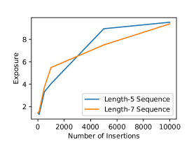
Figure 4: Exposure plot for our commercial word-level language model. Even with a canary inserted 10,000 times, exposure reaches only $10$: the model is $1,000\times$ more likely to generate this canary than another (random) possible phrase, but it is still not a very likely output, let alone the most likely.

In more detail, we inserted multiple canaries in the training data between 1 and 10,000 times (this does not impact model accuracy), and trained the full model on 32 GPUs over a billion sequences. Figure 4 contains the results of this analysis.

(Note: The measured exposure values are lower than in most of other experiments due to the vast quantity of training data; the model is therefore exposed to the same canary less often than in models trained for a large number of epochs.)

When we compute the exposure of each canary, we find that when secrets are very rare (i.e., one in a billion) the model shows no signs of memorization; the measured exposure is negligible. When the canaries are inserted at higher frequencies, exposure begins to increase so that the inserted canaries become with $1000\times$ more likely than non-inserted canaries. However, even this higher exposure doesn’t come close to allowing discovery of canaries using our extraction algorithms (see Section 8), let alone accidental discovery.

Informed by these results, limits can be placed on the incidence of unique sequences and sampling rates, and clipping and differential-privacy noise (see Section 9.3) can be added to the training process, such that privacy is empirically protected by eliminating any measured signal of exposure.

6.2 Word-Level Language Model

Next we apply our technique to one of the current state-of-the-art world-level language models [35]. We train this model on WikiText-103 dataset [34], a $500$MB cleaned subset of English Wikipedia. We do not alter the open-source implementation provided by the authors; we insert a canary five times and train the model with different hyperparameters. We choose as a format a sequence of eight words random selected from the space of any of the 267,735 different words in the model’s vocabulary (i.e., that occur in the training dataset).

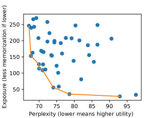
Figure 5: The results of applying our testing methodology to a word-level language model [35] inserting a canary five times. An exposure of $144$ indicates extraction should be possible. We train many models each with different hyperparameters and find vast differences in the level of memorization. The highest utility model memorizes the canary to such a degree it can be extracted. Other models that reach similar utility exhibit less memorization. A practitioner would prefer one of the models on the Pareto frontier, which we highlight.

We train many models with different hyperparameters and report in Figure 5 the utility as measured by test perplexity (i.e., the exponential of the model loss) against the measured exposure for the inserted canary. While memorization and utility are not highly correlated (r=-0.32), this is in part due to the fact that many choices of hyperparameters give poor utility. We show the Pareto frontier with a solid line.

6.3 Character-Level Language Model

While previously we applied a small character-level model to the Penn Treebank dataset and measured the exposure of a random number sequence, we now confirm that the results from Section 6.2 hold true for a state-of-the-art character-level model. To verify this, we apply the character-level model from [35] to the PTB dataset.

As expected, based on our experiment in Section 3, we find that a character model model is less prone to memorizing a random sequence of words than a random sequence of numbers. However, the character-level model still does memorize the inserted random words: it reaches an exposure of $60$ (insufficient to extract) after $16$ insertions, in contrast to the word-models from the previous section that showed exposures much higher than this at only $5$ insertions.

6.4 Neural Machine Translation

In addition to language modeling, another common use of generative sequence models is Neural Machine Translation [3]. NMT is the process of applying a neural network to translate from one language to another. We demonstrate that unintentional memorization is also a concern on this task, and because the domain is different, NMT also provides us with a case study for designing a new perplexity measure.

NMT receives as input a vector of words $x_{i}$ in one language and outputs a vector of words $y_{i}$ in a different language. It achieves this by learning an encoder $e:\vec{x}\to\mathbb{R}^{k}$ that maps the input sentence to a “thought vector” that represents the meaning of the sentence. This $k$-dimensional vector is then fed through a decoder $d:\mathbb{R}^{k}\to\vec{y}$ that decodes the thought vector into a sentence of the target language.

Internally, the encoder is a recurrent neural network that maintains a state vector and processes the input sequence one word at a time. The final internal state is then returned as the thought vector $v\in\mathbb{R}^{k}$. The decoder is then initialized with this thought vector, which the decoder uses to predict the translated sentence one word at a time, with every word it predicts being fed back in to generate the next.

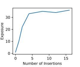
Figure 6: Exposure of a canary inserted in a Neural Machine Translation model. When the canary is inserted four times or more, it is fully memorized.

We take our NMT model directly from the TensorFlow Model Repository [12]. We follow the steps from the documentation to train an English-Vietnamese model, trained on 100k sentences pairs. We add to this dataset an English canary of the format “My social security number is - - ” and a corresponding Vietnamese phrase of the same format, with the English text replaced with the Vietnamese translation, and insert this canary translation pair.

Because we have changed problem domains, we must define a new perplexity measure. We feed the initial source sentence $\vec{x}$ through the encoder to compute the thought vector. To compute the perplexity of the source sentence mapping to the target sentence $\vec{y}$, instead of feeding the output of one layer to the input of the next, as we do during standard decoding, we instead always feed $y_{i}$ as input to the decoder’s hidden state. The perplexity is then computed by taking the log-probability of each output being correct, as is done on word models. Why do we make this change to compute perplexity? If one of the early words is guessed incorrectly and we feed it back in to the next layer, the errors will compound and we will get an inaccurate perplexity measure. By always feeding in the correct output, we can accurately judge the perplexity when changing the last few tokens. Indeed, this perplexity definition is already implemented in the NMT code where it is used to evaluate test accuracy. We re-purpose it for performing our memorization evaluation.

Under this new perplexity measure, we can now compute the exposure of the canary. We summarize these results in Figure 6. By inserting the canary only once, it already occurs $1000\times$ more likely than random chance, and after inserting four times, it is completely memorized.

7 Characterizing Unintended Memorization

While the prior sections clearly demonstrate that unintended memorization is a problem, we now investigate why and how models unintentionally memorize training data by applying the testing methodology described above.

Experimental Setup:

Unless otherwise specified, the experiments in this section are performed using the same LSTM character-level model discussed in Section 3 trained on the PTB dataset with a single canary inserted with the format “the random number is ” where the maximum exposure is $\log_{2}(10^{9})\approx 30$.

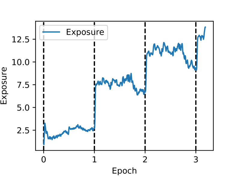
Figure 7: Exposure as a function of training time. The exposure spikes after the first mini-batch of each epoch (which contains the artificially inserted canary), and then falls overall during the mini-batches that do not contain it.

7.1 Memorization Throughout Training

To begin we apply our testing methodology to study a simple question: how does memorization progress during training?

We insert the canary near the beginning of the Penn Treebank dataset, and disable shuffling, so that it occurs at the same point within each epoch. After every mini-batch of training, we estimate the exposure of the canary. We then plot the exposure of this canary as the training process proceeds.

Figure 7 shows how unintended memorization begins to occur over the first three epochs of training on $10\%$ of the training data. Each time the model trains on a mini-batch that contains the canary, the exposure spikes. For the remaining mini-batches (that do not contain the canary) the exposure randomly fluctuates and sometimes decreases due to the randomness in stochastic gradient descent.

It is also interesting to observe that memorization begins to occur after only one epoch of training: at this point, the exposure of the canary is already 3, indicating the canary is $2^{3}=8\times$ more likely to occur than another random sequence chosen with the same format. After three epochs, the exposure is $8$: access to the model reduces the number of guesses that would be needed to guess the canary by over $100\times$.

7.2 Memorization versus Overtraining

Next, we turn to studying how unintended memorization relates to overtraining. Recall we use the word overtraining to refer to a form of overfitting as a result of training too long.

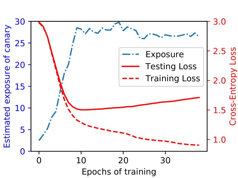
Figure 8: Comparing training and testing loss to exposure across epochs on $5\%$ of the PTB dataset . Testing loss reaches a minimum at 10 epochs, after which the model begins to over-fit (as seen by training loss continuing to decrease). Exposure also peaks at this point, and decreases afterwards.

Figure 8 plots how memorization occurs during training on a sample of $5\%$ of the PTB dataset, so that it quickly overtrains. The first few epochs see the testing loss drop rapidly, until the minimum testing loss is achieved at epoch 10. After this point, the testing loss begins to increase—the model has overtrained.

Comparing this to the exposure of the canary, we find an inverse relationship: exposure initially increases rapidly, until epoch 10 when the maximum amount of memorization is achieved. Surprisingly, the exposure does not continue increasing further, even though training continues. In fact, the estimated exposure at epoch 10 is actually higher than the estimated exposure at epoch 40 (with p-value $p<.001$). While this is interesting, in practice it has little effect: the rank of this canary is $1$ for all epochs after 10.

Taken together, these results are intriguing. They indicate that unintended memorization seems to be a necessary component of training: exposure increases when the model is learning, and does not when the model is not. This result confirms one of the findings of Tishby and Schwartz-Ziv [43] and Zhang et al. [57], who argue that neural networks first learn to minimize the loss on the training data by memorizing it.

7.3 Additional Memorization Experiments

Appendix A details some further memorization experiments.

8 Validating Exposure with Extraction

How accurate is the exposure metric in measuring memorization? We study this question by developing an extraction algorithm that we show can efficiently extract training data from a model when our exposure metric indicates this should be possible (i.e., when the exposure is greater than $\log_{2}{|\mathcal{R}|}$).

8.1 Efficient Extraction Algorithm

Proof of concept brute-force search:

We begin with a simple brute-force extraction algorithm that enumerates all possible sequences, computes their perplexity, and returns them in order starting from the ones with lowest perplexity. Formally, we compute $\mathop{\text{arg min}}_{r\in\mathcal{R}}\mathrm{Px}_{\theta}(s[r])$. While this approach might be effective at validating our exposure metric accurately captures what it means for a sequence to be memorized, it is unable to do so when the space $\mathcal{R}$ is large. For example, brute-force extraction over the space of credit card numbers ($10^{16}$) would take 4,100 commodity GPU-years.

Shortest-path search:

In order to more efficiently perform extraction, we introduce an improved search algorithm, a modification of Dijkstra’s algorithm, that in practice reduces the complexity by several orders of magnitude.

To begin, observe it is possible to organize all possible partial strings generated from the format $s$ as a weighted tree, where the empty string is at the root. A partial string $b$ is a child of $a$ if $b$ expands $a$ by one token $t$ (which we denote by $b=a@t$). We set the edge weight from $a$ to $b$ to $-\log{\mathbf{Pr}(t|f_{\theta}(a))}$ (i.e., the negative log-likelihood assigned by the model to the token $t$ following the sequence $a$).

Leaf nodes on the tree are fully-completed sequences. Observe that the total edge weight from the root $x_{1}$ to a leaf node $x_{n}$ is given by

$$\sum-\log_{2}{\mathbf{Pr}(x_{i}|f_{\theta}(x_{1}...x_{i-1}))}$$

$$=\mathrm{Px}_{\theta}(x_{1}...x_{n})$$ (By Definition 1)

Therefore, finding $s[r]$ minimizing the cost of the path is equivalent to minimizing its log-perplexity. Figure 9 presents an example to illustrate the idea. Thus, finding the sequence with lowest perplexity is equivalent to finding the lightest path from the root to a leaf node.

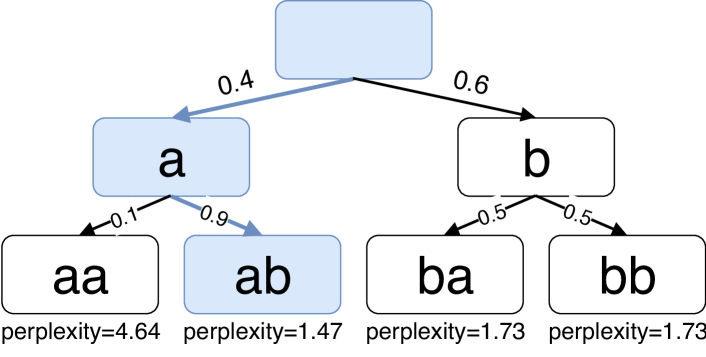
Figure 9: An example to illustrate the shortest path search algorithm. Each node represents one partially generated string. Each edge denotes the conditional probability $\mathbf{Pr}(x_{i}|x_{1}...x_{i-1})$. The path to the leaf with minimum perplexity is highlighted, and the log-perplexity is depicted below each leaf node.

Concretely, we implement a shortest-path algorithm directly inspired by Dijkstra’s algorithm [11] which computes the shortest distance on a graph with non-negative edge weights. The algorithm maintains a priority queue of nodes on the graph. To initialize, only the root node (the empty string) is inserted into the priority queue with a weight 0. In each iteration, the node with the smallest weight is removed from the queue. Assume the node is associated with a partially generated string $p$ and the weight is $w$. Then for each token $t$ such that $p@t$ is a child of $p$, we insert the node $p@t$ into the priority queue with $w-\log{\mathbf{Pr}(t|f_{\theta}(p))}$ where $-\log{\mathbf{Pr}(t|f_{\theta}(p))}$ is the weight on the edge from $p$ to $p@t$.

The algorithm terminates once the node pulled from the queue is a leaf (i.e., has maximum length). In the worst-case, this algorithm may enumerate all non-leaf nodes, (e.g., when all possible sequences have equal perplexity). However, empirically, we find shortest-path search enumerate from 3 to 5 orders of magnitude fewer nodes (as we will show).

During this process, the main computational bottleneck is computing the edge weights $-\log{\mathbf{Pr}(t|f_{\theta}(p))}$. A modern GPU can simultaneously evaluate a neural network on many thousand inputs in the same amount of time as it takes to evaluate one. To leverage this benefit, we pull multiple nodes from the priority queue at once in each iteration, and compute all edge weights to their children simultaneously. In doing so, we observe a $50\times$ to $500\times$ reduction in overall run-time.

Applying this optimization violates the guarantee that the first leaf node found is always the best. We compensate by counting the number of iterations required to find the first full-length sequence, and continuing that many iterations more before stopping. We then sort these sequences by log-perplexity and return the lowest value. While this doubles the number of iterations, each iteration is two orders of magnitude faster, and this results in a substantial increase in performance.

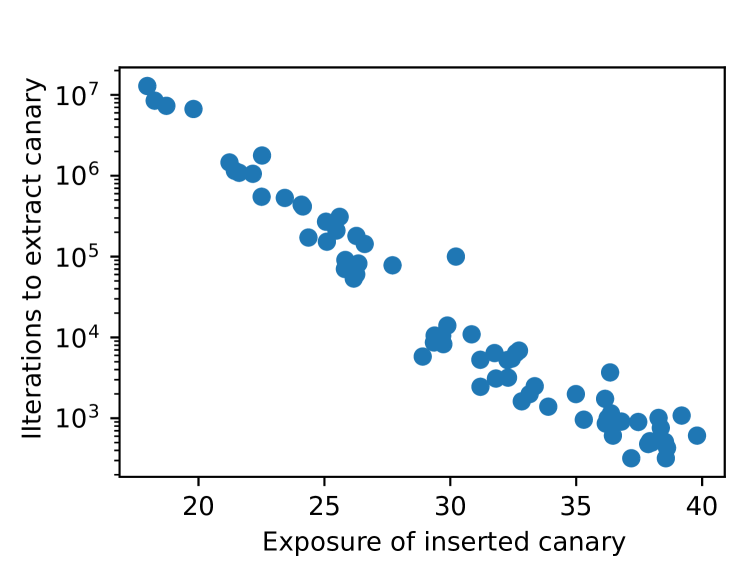
Figure 10: Number of iterations the shortest-path search requires before an inserted canary is returned, with $|\mathcal{R}|=2^{30}$. At exposure 30, when the canary is fully memorized, our algorithm requires over four orders of magnitude fewer queries compared to brute force.

8.2 Efficiency of Shortest-Path Search

We begin by again using our character level language model as a baseline, after inserting a single 9-digit random canary to the PTB dataset once. This model completely memorizes the canary: we find its exposure is over 30, indicating it should be extractable. We verify that it actually does have the lowest perplexity of all candidates canaries by enumerating all $10^{9}$.

Shortest path search:

We apply our shortest-path algorithm to this model and find that it takes only $10^{5}$ total queries: four orders of magnitude fewer than a brute-force approach takes.

Perhaps as is expected, we find that the shortest-path algorithm becomes more efficient when the exposure of the canary is higher. We train multiple different models containing a canary to different final exposure values (by varying model capacity and number of training epochs). Figure 10 shows the exposure of the canary versus the number of iterations the shortest path search algorithm requires to find it. The shortest-path search algorithm reduces the number of values enumerated in the search from $10^{9}$ to $10^{4}$ (a factor of $100,000\times$ reduction) when the exposure of the inserted phrase is greater than 30.

8.3 High Exposure Implies Extraction

Turning to the main purpose of our extraction algorithm, we verify that it actually means something when the exposure of a sequence is high. The underlying hypothesis of our work is that exposure is a useful measure for accurately judging when canaries have been memorized. We now validate that when the exposure of a phrase is high, we can extract the phrase from the model (i.e., there are not many false positives, where exposure is high but we can’t extract it). We train multiple models on the PTB dataset inserting a canary (drawn from a randomness space $|\mathcal{R}|\approx 2^{30}$) a varying number of times with different training regimes (but train all models to the same final test accuracy). We then measure exposure on each of these models and attempt to extract the inserted canary.

Figure 11 plots how exposure correlates with the success of extraction: extraction is always possible when exposure is greater than $33$ but never when exposure is less than $31$.

8.4 Enron Emails: Memorization in Practice

It is possible (although unlikely) that we detect memorization only because we have inserted our canaries artificially. To confirm this is not the case, we study a dataset that has many naturally-occurring secrets already in the training data. That is to say, instead of running experiments on data with the canaries we have artificially inserted and treated as “secrets”, we run experiments on a dataset where secrets are pre-existing.

Figure 11: Extraction is possible when the exposure indicates it should be possible: when $|\mathcal{R}|=2^{30}$, at an exposure of $30$ extraction quickly shifts from impossible to possible.

The Enron Email Dataset consists of several hundred thousand emails sent between employees of Enron Corporation, and subsequently released by the Federal Energy Regulatory Commission in its investigation of the company. The complete dataset consists of the full emails, with attachments. Many users sent highly sensitive information in these emails, including social security numbers and credit card numbers.

We pre-process this dataset by removing all attachments, and keep only the body of the email. We remove the text of the email that is being responded to, and filter out automatically-generated emails and emails sent to the entire company. We separate emails by sender, ranging from $1.7$MB to $5.6$MB (about the size of the PTB dataset) and train one character-level language model per user who has sent at least one secret. The language model we train is again a 2-layer LSTM, however to model the more complex nature of writing we increase the number of units in each layer to 1024. We again train to minimum validation loss.

User	Secret Type	Exposure	Extracted?
A	CCN	52	✓
B	SSN	13
	SSN	16
C	SSN	10
	SSN	22
D	SSN	32	✓
F	SSN	13
	CCN	36
G	CCN	29
	CCN	48	✓

Table 2: Summary of results on the Enron email dataset. Three secrets are extractable in $<1$ hour; all are heavily memorized.

We summarize our results in Table 2. Three of these secrets (that pre-exist in the data) are memorized to a degree that they can be extracted by our shortest-path search algorithm. When we run our extraction algorithm locally, it requires on the order of a few hours to extract the credit card and social security numbers. Note that it would be unfair to draw from this that an actual attack would only take a few hours: this local attack can batch queries to the model and does not include any remote querying in the run-time computation.

9 Preventing Unintended Memorization

As we have shown, neural networks quickly memorize secret data. This section evaluates (both the efficacy and impact on accuracy) three potential defenses against memorization: regularization, sanitization, and differential privacy.

9.1 Regularization

It might be reasonable to assume that unintended memorization is due to the model overtraining to the training data. To show this is not the case, we apply three state-of-the-art regularization approaches (weight decay [29], dropout [46], and quantization [26]) that help prevent overtraining (and overfitting) and find that none of these can prevent the canaries we insert from being extracted by our algorithms.

9.1.1 Weight Decay

Weight decay [29] is a traditional approach to combat overtraining. During training, an additional penalty is added to the loss of the network that penalizes model complexity.

Our initial language $600$k parameters and was trained on the $5$MB PTB dataset. It initially does not overtrain (because it does not have enough capacity). Therefore, when we train our model with weight decay, we do not observe any improvement in validation loss, or any reduction in memorization.

In order to directly measure the effect of weight decay on a model that does overtrain, we take the first $5\%$ of the PTB dataset and train our language model there. This time the model does overtrain the dataset without regularization. When we add $L_{2}$ regularization, we see less overtraining occur (i.e., the model reaches a lower validation loss). However, we observe no effect on the exposure of the canary.

9.1.2 Dropout

Dropout [46] is a regularization approach proposed that has been shown to effectively prevent overtraining in neural networks. Again, dropout does not help with the original model on the full dataset (and does not inhibit memorization).

We repeat the experiment above by training on $5\%$ of the data, this time with dropout. We vary the probability to drop a neuron from $0\%$ to $90\%$, and train ten models at each dropout rate to eliminate the effects of noise.

At dropout rates between $0\%$ and $20\%$, the final test accuracy of the models are comparable (Dropout rates greater than $30\%$ reduce test accuracy on our model). We again find that dropout does not statistically significantly reduce the effect of unintended memorization.

9.1.3 Quantization

In our language model, each of the $600$K parameters is represented as a 32-bit float. This puts the information theoretic capacity of the model at $2.4$MB, which is larger than the $1.7$MB size of the compressed PTB dataset. To demonstrate the model is not storing a complete copy of the training data, we show that the model can be compressed to be much smaller while maintaining the same exposure and test accuracy.

To do this, we perform weight quantization [26]: given a trained network with weights $\theta$, we force each weight to be one of only $256$ different values, so each parameter can be represented in 8 bits. As found in prior work, quantization does not significantly affect validation loss: our quantized model achieves a loss of $1.19$, compared to the original loss of $1.18$. Additionally, we find that the exposure of the inserted canary does not change: the inserted canary is still the most likely and is extractable.

9.2 Sanitization

Sanitization is a best practice for processing sensitive, private data. For example, we may construct blacklists and filter out sentences containing what may be private information from language models, or may remove all numbers from a model trained where only text is expected. However, one can not hope to guarantee that all possible sensitive sequences will be found and removed through such black-lists (e.g., due to the proliferation of unknown formats or typos).

We attempted to construct an algorithm that could automatically identify potential secrets by training two models on non-overlapping subsets of training data and removing any sentences where the perplexity between the two models disagreed. Unfortunately, this style of approach missed some secrets (and is unsound if the same secret is inserted twice).

While sanitization is always a best practice and should be applied at every opportunity, it is by no means a perfect defense. Black-listing is never a complete approach in security, and so we do not consider it to be effective here.

9.3 Differential Privacy

Differential privacy [13, 15, 16] is a property that an algorithm can satisfy which bounds the information it can leak about its inputs. Formally defined as follows.

Definition 5

A randomized algorithm $\mathcal{A}$ operating on a dataset $\mathcal{D}$ is $(\varepsilon,\delta)$-differentially private if

$$\mathbf{Pr}[\mathcal{A}(\mathcal{D})\in S]\leq\exp(\varepsilon)\cdot\mathbf{Pr}[\mathcal{A}(\mathcal{D}^{\prime})\in S]+\delta$$

for any set $S$ of possible outputs of $\mathcal{A}$, and any two data sets $\mathcal{D},\mathcal{D}^{\prime}$ that differ in at most one element.

Intuitively, this definition says that when adding or removing one element from the input data set, the output distribution of a differentially private algorithm does not change by much (i.e., by more than an a factor exponentially small in $\varepsilon$). Typically we set $\varepsilon=1$ and $\delta<{|\mathcal{X}|^{-1}}$ to give strong privacy guarantees. Thus, differential privacy is a desirable property to defend against memorization. Consider the case where $\mathcal{D}$ contains one occurrence of some secret training record $x$, and $\mathcal{D}^{\prime}=\mathcal{D}-\{x\}$. Imprecisely speaking, the output model of a differentially private training algorithm running over $\mathcal{D}$, which contains the secret, must be similar to the output model trained from $\mathcal{D}^{\prime}$, which does not contain the secret. Thus, such a model can not memorize the secret as completely.

We applied the differentially-private stochastic gradient descent algorithm (DP-SGD) from [1] to verify that differential privacy is an effective defense that prevents memorization. We used the initial, open-source code for DP-SGD to train our character-level language model from Section 3. We slightly modified this code to adapt it to recurrent neural networks and improved its baseline performance by replacing the plain SGD optimizer with an RMSProp optimizer, as it often gives higher accuracy than plain SGD [48].

The DP-SGD of [1] implements differential privacy by clipping the per-example gradient to a max norm and carefully adding Gaussian noise. Intuitively, if the added noise matches the clipping norm, every single, individual example will be masked by the noise, and cannot affect the weights of the network by itself. As more noise is added, relative to the clipping norm, the more strict the $\varepsilon$ upper-bound on the privacy loss that can be guaranteed.

			Test	Estimated	Extraction
	Optimizer	$\varepsilon$	Loss	Exposure	Possible?
With DP
	RMSProp	0.65	1.69	1.1
	RMSProp	1.21	1.59	2.3
	RMSProp	5.26	1.41	1.8
	RMSProp	89	1.34	2.1
	RMSProp	$2\times 10^{8}$	1.32	3.2
	RMSProp	$1\times 10^{9}$	1.26	2.8
	SGD	$\infty$	2.11	3.6
No DP
	SGD	N/A	1.86	9.5
	RMSProp	N/A	1.17	31.0	✓

Table 3: The RMSProp models trained with differential privacy do not memorize the training data and always have lower testing loss than a non-private model trained using standard SGD techniques. (Here, $\varepsilon=\infty$ indicates the moments accountant returned an infinite upper bound on $\varepsilon$.)

We train seven differentially private models using various values of $\varepsilon$ for $100$ epochs on the PTB dataset augmented with one canary inserted. Training a differentially private algorithm is known to be slower than standard training; our implementation of this algorithm is $10-100\times$ slower than standard training. For computing the $(\varepsilon,\delta)$ privacy budget we use the moments accountant introduced in [1]. We set $\delta=10^{-9}$ in each case. The gradient is clipped by a threshold $L=10.0$. We initially evaluate two different optimizers (the plain SGD used by authors of [1] and RMSProp), but focus most experiments on training with RMSProp as we observe it achieves much better baseline results than SGD. Table 3 shows the evaluation results.

The differentially-private model with highest utility (the lowest loss) achieves only $10\%$ higher test loss than the baseline model trained without differential privacy. As we decrease $\varepsilon$ to $1.0$, the exposure drops to $1$, the point at which this canary is no more likely than any other. This experimentally verifies what we already expect to be true: DP-RMSProp fully eliminates the memorization effect from a model. Surprisingly, however, this experiment also show that a little-bit of carefully-selected noise and clipping goes a long way—as long as the methods attenuate the signal from unique, secret input data in a principled fashion. Even with a vanishingly-small amount of noise, and values of $\varepsilon$ that offer no meaningful theoretical guarantees, the measured exposure is negligible.

Our experience here matches that of some related work. In particular, other, recent measurement studies have also found an orders-of-magnitude gap between the empirical, measured privacy loss and the upper-bound $\varepsilon$ DP guarantees—with that gap growing (exponentially) as $\varepsilon$ becomes very large [27]. Also, without modifying the training approach, improved proof techniques have been able to improve guarantees by orders of magnitude, indicating that the analytic $\varepsilon$ is not a tight upper bound. Of course, these improved proof techniques often rely on additional (albeit realistic) assumptions, such as that random shuffling can be used to provide unlinkability [17] or that the intermediate model weights computed during training can be hidden from the adversary [18]. Our $\varepsilon$ calculation do not utilize these improved analysis techniques.

10 Related Work and Conclusions

There has been a significant amount of related work in the field of privacy and machine learning.

Membership Inference.

Prior work has studied the privacy implications of training on private data. Given a neural network $f(\cdot)$ trained on training data $\mathcal{X}$, and an instance $x$, it is possible to construct a membership inference attack [42] that answers the question “Is $x$ a member of $\mathcal{X}$?”.

Exposure can be seen as an improvement that quantifies how much memorization has occurred (and not just if it has). We also show that given only access to $f(\cdot)$, we extract an $x$ so that $x\in\mathcal{X}$ (and not just infer if it is true that $x\in\mathcal{X}$), at least in the case of generative sequence models.

Membership inference attacks have seen further study, including examining why membership inference is possible [50], or mounting inference attacks on other forms of generative models [23]. Further work shows how to use membership inference attacks to determine if a model was trained by using any individual user’s personal information [45]. These research directions are highly important and orthogonal to ours: this paper focuses on measuring unintended memorization, and not on any specific attacks or membership inference queries. Indeed, the fact that membership inference is possible is also highly related to unintended memorization.

More closely related to our paper is work which produces measurements for how likely it is that membership inference attacks will be possible [30] by developing the Differential Training Privacy metric for cases when differentially private training will not be possible.

Generalization in Neural Networks.

Zhang et al. [57] demonstrate that standard models can be trained to perfectly fit completely random data. Specifically, the authors show that the same architecture that can classify MNIST digits correctly with $99.5\%$ test accuracy can also be trained on completely random data to achieve $100\%$ train data accuracy (but clearly poor test accuracy). Since there is no way to learn to classify random data, the only explanation is that the model has memorized all training data labels.

Recent work has shown that overtraining can directly lead to membership inference attacks [54]. Our work indicates that even when we do not overtrain our models on the training data, unintentional memorization remains a concern.

Training data leakages.

Ateniese et al. [2] show that if an adversary is given access to a remote machine learning model (e.g., support vector machines, hidden Markov models, neural networks, etc.) that performs better than their own model, it is often possible to learn information about the remote model’s training data that can be used to improve the adversary’s own model. In this work the authors “are not interested in privacy leaks, but rather in discovering anything that makes classifiers better than others.” In contrast, we focus only on the problem of private training data.

Backdoor (intentional) memorization.

Song et al.  [44] also study training data extraction. The critical difference between their work and ours is that in their threat model, the adversary is allowed to influence the training process and intentionally back-doors the model to leak training data. They are able to achieve incredibly powerful attacks as a result of this threat model. In contrast, in our paper, we show that memorization can occur, and training data leaked, even when there is not an attacker present intentionally causing a back-door.

Model stealing

studies a related problem to training data extraction: under a black-box threat model, model stealing attempts to extract the parameters $\theta$ (or parameters similar to them) from a remote model, so that the adversary can have their own copy [49]. While model extraction is designed to steal the parameters $\theta$ of the remote model, training data extraction is designed to extract the training data that was used to generate $\theta$. That is, even if we were given direct access to $\theta$ it is still difficult to perform training data extraction.

Later work extended model-stealing attacks to hyperparameter-stealing attacks [51]. These attacks are highly effective, but are orthogonal to the problems we study in this paper. Related work [39] also makes a similar argument that it can be useful to steal hyperparameters in order to mount more powerful attacks on models.

Model inversion

[19, 20] is an attack that learns aggregate statistics of the training data, potentially revealing private information. For example, consider a face recognition model: given an image of a face, it returns the probability the input image is of some specific person. Model inversion constructs an image that maximizes the confidence of this classifier on the generated image; it turns out this generated image often looks visually similar to the actual person it is meant to classify. No individual training instances are leaked in this attack, only an aggregate statistic of the training data (e.g., what the average picture of a person looks like). In contrast, our extraction algorithm reveals specific training examples.

Private Learning.

Along with the attacks described above, there has been a large amount of effort spent on training private machine learning algorithms. The centerpiece of these defenses is often differential privacy [13, 15, 16, 7, 1]. Our analysis in Section 9.3 directly follows this line of work and we confirm that it empirically prevents the exposure of secrets. Other related work [41] studies membership attacks on differentially private training, although in the setting of a distributed honest-but-curious server.

Other related work [38] studies how to apply adversarial regularization to reduce the risk of black-box membership inference attacks, although using different approach than taken by prior work. We do not study this type of adversarial regularization in this paper, but believe it would be worth future analysis in follow-up work.

10.1 Limitations and Future Work

This work in this paper represents a practical step towards measuring unintended memorization in neural networks. There are several areas where our work is limited in scope:

• Our paper only considers generative models, as they are models that are likely to be trained on sensitive information (credit card numbers, names, addresses, etc). Although, our approach here will apply directly to any type of model with a defined measure of perplexity, further work is required to handle other types of machine-learning models, such as image classifiers.

• Our extraction algorithm presented here was designed to validate that canaries with a high exposure actually correspond to some real notion of the potential to extract that canary, and by analogy other possible secrets present in training data. However, this algorithm has assumptions that make it ill-suited to real-world attacks. To begin, real-world models usually only return the most likely (i.e., the arg max) output. Furthermore, we assume knowledge of the surrounding context and possible values of the canary, which may not hold true in practice.

• Currently, we only make use of the input-output behavior of the model to compute the exposure of sequences. When performing our testing, we have full white-box access including the actual weights and internal activations of the neural network. This additional information might be used to develop stronger measures of memorization.

We hope future work will build on ours to develop further metrics for testing unintended memorization of unique training data details in machine-learning models.

10.2 Conclusions

The fact that deep learning models overfit and overtrain to their training data has been extensively studied [57]. Because neural network training should minimize loss across all examples, training must involve a form of memorization. Indeed, significant machine learning research has been devoted to developing techniques to counteract this phenomenon [46].

In this paper we consider the related phenomenon of what we call unintended memorization: deep learning models (in particular, generative models) appear to often memorize rare details about the training data that are completely unrelated to the intended task while the model is still learning the underlying behavior (i.e., while the test loss is still decreasing). As we show, traditional approaches to avoid overtraining do not inhibit unintentional memorization.

Such unintended memorization of rare training details may raise significant privacy concerns when sensitive data is used to train deep learning models. Most worryingly, such memorization can happen even for examples that are present only a handful of times in the training data, especially when those examples are outliers in the data distribution; this is true even for language models that make use of state-of-the-art regularization techniques to prevent traditional forms of overfitting and overtraining.

To date, no good method exists for helping practitioners measure the degree to which a model may have memorized aspects of the training data. Towards this end, we develop exposure: a metric which directly quantifies the degree to which a model has unintentionally memorized training data. We use exposure as the basis of a testing methodology whereby we insert canaries (orthogonal to the learning task) into the training data and measure their exposure. By design, exposure is a simple metric to implement, often requiring only a few dozen lines of code. Indeed, our metric has, with little effort, been applied to construct regression tests for Google’s Smart Compose [8]: a large industrial language model trained on a privacy-sensitive text corpus.

In this way, we contribute a technique that can usefully be applied to aid machine learning practitioners throughout the training process, from curating the training data, to selecting the model architecture and hyperparameters, all the way to extracting meaning from the $\varepsilon$ values given by applying the provably private techniques of differentially private stochastic gradient descent.

Appendix A Additional Memorization Experiments

A.1 Across Different Architectures

We evaluate different neural network architectures in Table 4 again on the PTB dataset, and find that all of them unintentionally memorize. We observe that the two recurrent neural networks, i.e., LSTM [24] and GRU [9], demonstrate both the highest accuracy (lowest loss) and the highest exposure. Convolutional neural networks’ accuracy and exposure are both lower. Therefore, through this experiment, we show that the memorization is not only an issue to one particular architecture, but appears to be common to neural networks.

Architecture	Layers	Units	Test Loss	Exposure
GRU	1	370	1.18	36
GRU	2	235	1.18	37
LSTM	1	320	1.17	38
LSTM	2	200	1.16	35
CNN	1	436	1.29	24
CNN	2	188	1.28	19
CNN	4	122	1.25	22
WaveNet	2	188	1.24	18
WaveNet	4	122	1.25	20

Table 4: Exposure of a canary for various model architectures. All models have 620K (+/- 5K) parameters and so have the same theoretical capacity. Convolutional neural networks (CNN/WaveNet) perform less well at the language modeling task, and memorize the canary to a lesser extent.

A.2 Across Training Strategies

There are various settings for training strategies and techniques that are known to impact the accuracy of the final model. We briefly evaluate the impact that each of these have on the exposure of the inserted canary.

Batch Size.

In stochastic gradient descent, we train on minibatches of multiple examples simultaneously, and average their gradients to update the model parameters. This is usually done for computational efficiency—due to their parallel nature, modern GPUs can evaluate a neural network on many thousands of inputs simultaneously.

To evaluate the effect of the batch size on memorization, we train our language model with different capacity (i.e., number of LSTM units) and batch size, ranging from $16$ to $1024$. (At each batch size for each number of units, we train 10 models and average the results.) All models with the same number of units reach nearly identical final training loss and testing loss. However, the models with larger batch size exhibit significantly more memorization, as shown in Table 5. This experiment provides additional evidence for prior work which has argued that using a smaller batch size yields more generalizable models [25]; however we ensure that all models reach the same final accuracy.

While this does give a method of reducing memorization for some models, it unfortunately comes at a significant cost: training with a small batch can be prohibitively slow, as it may prevent parallelizing training across GPUs (and servers, in a decentralized fashion).

Shuffling, Bagging, and Optimization Method.

Given a fixed batch-size, we examine how other choices impact memorization. We train our model with different optimizers: SGD, Momentum SGD, RMSprop [48], Adagrad [14], Adadelta [56], and Adam [28]; and with either shuffling, or bagging (where minibatches are sampled with replacement).

Not all models converge to the same final test accuracy. However, when we control for the final test accuracy by taking a checkpoint from an earlier epoch from those models that perform better, we found no statistically significant difference in the exposure of the canary with any of these settings; we therefore do not include these results.

Batch Size		Number of LSTM Units
		50	100	150	200	250
	16	1.7	4.3	6.9	9.0	6.4
	32	4.0	6.2	14.4	14.1	14.6
	64	4.8	11.7	19.2	18.9	21.3
	128	9.9	14.0	25.9	32.5	35.4
	256	12.3	21.0	26.4	28.8	31.2
	512	14.2	21.8	30.8	26.0	26.0
	1024	15.7	23.2	26.7	27.0	24.4

Table 5: Exposure of models trained with varying model sizes and batch sizes. Models of the same size trained for the same number of epochs and reached similar test loss. Larger batch sizes, and larger models, both increase the amount of memorization. The largest memorization in each column is highlighted in italics bold, the second largest in bold.

A.3 Across Formats and Context

We find that the context we are aware of affects our ability to detect whether or not memorization has occurred.

In our earlier experiments we computed exposure with the prefix “The random number is” and then placing the randomness as a suffix. What if instead we knew a suffix, and the randomness was a prefix? Alternatively, what if the randomness had a unique structure (e.g., SSNs have dashes)?

We find that the answer is yes: additional knowledge about the format of the canary increases our ability to detect it was memorized. To show this, we study different insertion formats, along with the exposure of the given canary after 5 and 10 epochs of training in Table 6, averaged across ten models trained with each of the formats.

Format	Exposure at Epoch
	5	10
	5.0	6.1
$\langle$s$\rangle$	6.3	7.1
$\langle$e$\rangle$	5.0	6.8
$\langle$s$\rangle$ $\langle$e$\rangle$	6.1	7.5
- -	5.1	9.5
- - - - - - - -	5.2	11.1

Table 6: Exposure of canaries when the we are aware of different amounts of surrounding context ($\langle$s$\rangle$ and $\langle$e$\rangle$ are in practice unique context characters of five random characters). The exposure is computed at epoch 5 and 10, before the models completely memorize the inserted canary.

For the first four rows of Table 6, we use the same model, but compute the exposure using different levels of context. This ensures that it is only our ability to detect exposure that changes. For the remaining two rows, because the format has changed, we train separate models. We find that increasing the available context also increases the exposure, especially when inner context is available; this additional context becomes increasingly important as training proceeds.

References

- [1] Martín Abadi, Andy Chu, Ian Goodfellow, H Brendan McMahan, Ilya Mironov, Kunal Talwar, and Li Zhang. Deep learning with differential privacy. In ACM CCS, 2016.
- [2] Giuseppe Ateniese, Luigi V Mancini, Angelo Spognardi, Antonio Villani, Domenico Vitali, and Giovanni Felici. Hacking smart machines with smarter ones: How to extract meaningful data from machine learning classifiers. International Journal of Security and Networks, 2015.
- [3] D Bahdanau, K Cho, and Y Bengio. Neural machine translation by jointly learning to align and translate. ICLR, 2015.
- [4] Yoshua Bengio, Réjean Ducharme, Pascal Vincent, and Christian Jauvin. A neural probabilistic language model. JMLR, 2003.
- [5] James Bradbury, Stephen Merity, Caiming Xiong, and Richard Socher. Quasi-recurrent neural networks. arXiv preprint arXiv:1611.01576, 2016.
- [6] Lord Castleton. Review: Amazon’s ‘Patriot’ is the best show of the year. 2017. Pajiba. http://www.pajiba.com/tv_reviews/review-amazons-patriot-is-the-best-show-of -the-year.php.
- [7] Kamalika Chaudhuri and Claire Monteleoni. Privacy-preserving logistic regression. In NIPS, 2009.
- [8] Mia Xu Chen, Benjamin N Lee, Gagan Bansal, Yuan Cao, Shuyuan Zhang, Justin Lu, Jackie Tsay, Yinan Wang, Andrew M Dai, Zhifeng Chen, et al. Gmail smart compose: Real-time assisted writing. arXiv preprint arXiv:1906.00080, 2019.
- [9] Junyoung Chung, Caglar Gulcehre, KyungHyun Cho, and Yoshua Bengio. Empirical evaluation of gated recurrent neural networks on sequence modeling. NIPS Workshop, 2014.
- [10] Joseph Conrad. The Secret Sharer. EBook #220. Project Gutenberg, 2009. Originally published in Harper’s Magazine, 1910.
- [11] T Cormen, C Leiserson, R Rivest, and C Stein. Introduction to Algorithms. MIT Press, 2009.
- [12] TensorFlow Developers. Tensorflow neural machine translation tutorial. https://github.com/tensorflow/nmt, 2017.
- [13] Irit Dinur and Kobbi Nissim. Revealing information while preserving privacy. In Proceedings of the twenty-second ACM SIGMOD-SIGACT-SIGART symposium on Principles of database systems. ACM, 2003.
- [14] John Duchi, Elad Hazan, and Yoram Singer. Adaptive subgradient methods for online learning and stochastic optimization. Journal of Machine Learning Research, 12(Jul):2121–2159, 2011.
- [15] C Dwork, F McSherry, K Nissim, and A Smith. Calibrating noise to sensitivity in private data analysis. In TCC, volume 3876, 2006.
- [16] Cynthia Dwork. Differential privacy: A survey of results. In Intl. Conf. on Theory and Applications of Models of Computation, 2008.
- [17] Úlfar Erlingsson, Vitaly Feldman, Ilya Mironov, Ananth Raghunathan, Kunal Talwar, and Abhradeep Thakurta. Amplification by shuffling: From local to central differential privacy via anonymity. In Proceedings of the Thirtieth Annual ACM-SIAM Symposium on Discrete Algorithms, pages 2468–2479. SIAM, 2019.
- [18] Vitaly Feldman, Ilya Mironov, Kunal Talwar, and Abhradeep Thakurta. Privacy amplification by iteration. In IEEE FOCS, 2018.
- [19] Matt Fredrikson, Somesh Jha, and Thomas Ristenpart. Model inversion attacks that exploit confidence information and basic countermeasures. In ACM CCS, 2015.
- [20] Matthew Fredrikson, Eric Lantz, Somesh Jha, Simon Lin, David Page, and Thomas Ristenpart. Privacy in pharmacogenetics: An end-to-end case study of personalized Warfarin dosing. In USENIX Security Symposium, pages 17–32, 2014.
- [21] Ian Goodfellow, Yoshua Bengio, Aaron Courville, and Yoshua Bengio. Deep learning, volume 1. MIT press Cambridge, 2016.
- [22] Priya Goyal, Piotr Dollár, Ross Girshick, Pieter Noordhuis, Lukasz Wesolowski, Aapo Kyrola, Andrew Tulloch, Yangqing Jia, and Kaiming He. Accurate, large minibatch SGD: Training ImageNet in 1 hour. arXiv preprint arXiv:1706.02677, 2017.
- [23] Jamie Hayes, Luca Melis, George Danezis, and Emiliano De Cristofaro. LOGAN: Evaluating privacy leakage of generative models using generative adversarial networks. PETS, 2018.
- [24] Sepp Hochreiter and Jürgen Schmidhuber. Long short-term memory. Neural computation, 9(8):1735–1780, 1997.
- [25] Elad Hoffer, Itay Hubara, and Daniel Soudry. Train longer, generalize better: Closing the generalization gap in large batch training of neural networks. arXiv preprint arXiv:1705.08741, 2017.
- [26] I Hubara, M Courbariaux, D Soudry, R El-Yaniv, and Y Bengio. Quantized neural networks: Training neural networks with low precision weights and activations. arXiv preprint arXiv:1609.07061, 2016.
- [27] Bargav Jayaraman and David Evans. Evaluating differentially private machine learning in practice. In USENIX Security Symposium, 2019.
- [28] Diederik Kingma and Jimmy Ba. Adam: A method for stochastic optimization. ICLR, 2015.
- [29] Anders Krogh and John A Hertz. A simple weight decay can improve generalization. In NIPS, pages 950–957, 1992.
- [30] Yunhui Long, Vincent Bindschaedler, and Carl A Gunter. Towards measuring membership privacy. arXiv preprint 1712.09136, 2017.
- [31] Mitchell P Marcus, Mary Ann Marcinkiewicz, and Beatrice Santorini. Building a large annotated corpus of English: The Penn Treebank. Computational linguistics, 19(2):313–330, 1993.
- [32] Frank J Massey Jr. The Kolmogorov-Smirnov test for goodness of fit. Journal of the American statistical Association, 46(253), 1951.
- [33] Joseph Menn. Amazon posts a tell-all of buying lists. 1999. Los Angeles Times. https://www.latimes.com/archives/la-xpm-1999-aug-26-fi-3760-story.html.
- [34] Stephen Merity, Nitish Shirish Keskar, and Richard Socher. Regularizing and optimizing LSTM language models. arXiv preprint arXiv:1708.02182, 2017.
- [35] Stephen Merity, Nitish Shirish Keskar, and Richard Socher. An analysis of neural language modeling at multiple scales. arXiv preprint arXiv:1803.08240, 2018.
- [36] Tomas Mikolov, Martin Karafiát, Lukas Burget, Jan Cernockỳ, and Sanjeev Khudanpur. Recurrent neural network based language model. In Interspeech, volume 2, page 3, 2010.
- [37] Randall Munroe. Predictive models. https://xkcd.com/2169/, 2019.
- [38] Milad Nasr, Reza Shokri, and Amir Houmansadr. Machine learning with membership privacy using adversarial regularization. In Proceedings of the 2018 ACM SIGSAC Conference on Computer and Communications Security, pages 634–646. ACM, 2018.
- [39] Seong Joon Oh, Max Augustin, Mario Fritz, and Bernt Schiele. Towards reverse-engineering black-box neural networks. In ICLR, 2018.
- [40] A O’hagan and Tom Leonard. Bayes estimation subject to uncertainty about parameter constraints. Biometrika, 63(1), 1976.
- [41] Le Trieu Phong, Yoshinori Aono, Takuya Hayashi, Lihua Wang, and Shiho Moriai. Privacy-preserving deep learning: Revisited and enhanced. In International Conference on Applications and Techniques in Information Security, pages 100–110. Springer, 2017.
- [42] Reza Shokri, Marco Stronati, Congzheng Song, and Vitaly Shmatikov. Membership inference attacks against machine learning models. In IEEE Symposium on Security and Privacy, 2017.
- [43] Ravid Shwartz-Ziv and Naftali Tishby. Opening the black box of deep neural networks via information. arXiv preprint 1703.00810, 2017.
- [44] Congzheng Song, Thomas Ristenpart, and Vitaly Shmatikov. Machine learning models that remember too much. In ACM CCS, 2017.
- [45] Congzheng Song and Vitaly Shmatikov. The natural auditor: How to tell if someone used your words to train their model. arXiv preprint arXiv:1811.00513, 2018.
- [46] Nitish Srivastava, Geoffrey E Hinton, Alex Krizhevsky, Ilya Sutskever, and Ruslan Salakhutdinov. Dropout: A simple way to prevent neural networks from overfitting. JMLR, 15(1):1929–1958, 2014.
- [47] Igor V. Tetko, David J. Livingstone, and Alexander I. Luik. Neural network studies. 1. Comparison of overfitting and overtraining. Journal of Chemical Information and Computer Sciences, 35(5):826–833, 1995.
- [48] Tijmen Tieleman and Geoffrey Hinton. Lecture 6.5-rmsprop: Divide the gradient by a running average of its recent magnitude. COURSERA: Neural networks for machine learning, 4(2):26–31, 2012.
- [49] Florian Tramèr, Fan Zhang, Ari Juels, Michael K Reiter, and Thomas Ristenpart. Stealing machine learning models via prediction APIs. In USENIX Security Symposium, pages 601–618, 2016.
- [50] Stacey Truex, Ling Liu, Mehmet Emre Gursoy, Lei Yu, and Wenqi Wei. Towards demystifying membership inference attacks. arXiv preprint arXiv:1807.09173, 2018.
- [51] Binghui Wang and Neil Zhenqiang Gong. Stealing hyperparameters in machine learning. arXiv preprint arXiv:1802.05351, 2018.
- [52] Yonghui Wu, Mike Schuster, Zhifeng Chen, Quoc V Le, Mohammad Norouzi, Wolfgang Macherey, Maxim Krikun, Yuan Cao, Qin Gao, Klaus Macherey, et al. Google’s neural machine translation system: Bridging the gap between human and machine translation. arXiv preprint arXiv:1609.08144, 2016.
- [53] Yuanshun Yao, Bimal Viswanath, Jenna Cryan, Haitao Zheng, and Ben Y Zhao. Automated crowdturfing attacks and defenses in online review systems. ACM CCS, 2017.
- [54] Samuel Yeom, Irene Giacomelli, Matt Fredrikson, and Somesh Jha. Privacy risk in machine learning: Analyzing the connection to overfitting. In 2018 IEEE 31st Computer Security Foundations Symposium (CSF), pages 268–282. IEEE, 2018.
- [55] Yang You, Igor Gitman, and Boris Ginsburg. Scaling SGD batch size to 32k for ImageNet training. arXiv preprint arXiv:1708.03888, 2017.
- [56] Matthew D Zeiler. ADADELTA: An adaptive learning rate method. arXiv preprint arXiv:1212.5701, 2012.
- [57] Chiyuan Zhang, Samy Bengio, Moritz Hardt, Benjamin Recht, and Oriol Vinyals. Understanding deep learning requires rethinking generalization. ICLR, 2017.