SCRank: Spammer and Celebrity Ranking in Directed Social Networks

Abstract.

Many online social networks allow directed edges: Alice can unilaterally add an “edge” to Bob, typically indicating some kind of interest in Bob, or in Bob’s content, without Bob necessarily reciprocating with an “add-back” edge that would have indicated Bob’s interest in Alice. This significantly affects the dynamics of interactions in the social network. Most importantly, we observe the rise of two distinctive classes of users, celebrities and follow spammers, who accrue unreciprocated directed links in two different directions: celebrities attract many unreciprocated incoming links, and follow spammers create many unreciprocated outgoing links. Identifying users in both of these two categories is an important problem since a user’s status as a celebrity or as a follow spammer is an important factor in abuse detection, user and content ranking, privacy choices, and other social network features.

In this paper we develop SCRank, an iterative algorithm that exploits a deep connection between these two categories, and classifies both celebrities and follow spammers using purely the social graph structure. We analyze SCRank both theoretically and experimentally. Our theoretical analysis shows that SCRank always decreases a potential function, and therefore converges to an approximate equilibrium point. We then use experimental evaluation on a real global-scale social network and on synthetically generated graphs to observe that the algorithm converges very quickly, and consistently to the same solution. Using synthetic data with built-in ground truth, we also experimentally show that the algorithm provides a good approximation to the built-in set of celebrities and spammers. Finally, we generalize our convergence proof to a general class of “scoring” algorithms, and prove that under mild conditions, algorithms in this class minimize a (non-trivial) potential function and therefore converge. We give several examples to demonstrate the versatility of this general framework and usefulness of our techniques in proving theoretical results on the convergence of iterative algorithms.

1. Introduction

Online social networks can be divided into two categories: undirected networks such as LinkedIn or (pre-2011) Facebook that require the consent of both endpoints in order to establish an edge, and directed ones such as Twitter, Google$+$, and Flickr, that allow one user to unilaterally create a directed edge to another, such as by “following” the latter’s public updates, without the latter creating a reciprocal (anti-parallel) edge to the former. As has been observed in practice (OReillyRant, ), this simple distinction significantly affects the dynamics of relationships in the system: undirected social networks like Facebook tend to cultivate socializing with friends, while directed networks like Twitter, interacting with content produced by strangers constitutes a significant portion of social interactions. In the latter case, there are often a few individuals who collect many incoming links, either because they are already famous outside the social network, or because they contribute exceptionally engaging, viral content to the social network’s ecosystem. These individuals are in a sense the “celebrities” of the network. On the other hand, we have nodes who accumulate many outgoing links to random strangers. We call these nodes “(follow) spammers”. As we explain below, identifying celebrities and spammers of a network are intertwined problems. This paper focuses on developing algorithms to identify users in these two classes.

The simplest approach to identify a spammer is to count the number of unreciprocated outgoing edges of each node and classify the node as a spammer if this number exceeds a threshold. The problem with this approach is that often a non-negligible number of regular users follow many celebrities, and this approach can identify such users as spammers. Similarly, classifying celebrities by counting the number of unreciprocated incoming links suffers from the problem that it can classify regular users who are targeted by many spammers (for example, by the virtue of having their name mentioned in a public, crawlable space) as celebrities. Instead, we focus on this recursive definition of celebrities and spammers:

• A celebrity is a node who is followed by many non-spammers.

• A spammer is a node who follows many non-celebrities.

This recursive definition hints at a natural iterative approach for finding celebrities and spammers. In the next section, we mathematically formulate the problem and the iterative algorithm, which we call SCRank. We then analyze the convergence properties of SCRank, both theoretically and experimentally, and argue that its output provides useful information. We will use a real-world data set from LiveJournal, as well as randomly generated data, to experimentally evalute the convergence properties of our algorithm. To evaluate the output of our algorithm, we use randomly generated data with built in ground-truth, and show that the algorithm can recover a significant portion of the ground truth efficiently and accurately.

Finally, in Section 5, we give a generalization of our potential function argument to a more general framework of scoring problems, and prove that for any scoring problem satisfying a mild symmetry and monotonicity assumption, a (non-trivial) potential function can be associated with the natural iterative algorithm for the problem, and therefore the iterative algorithm provably converges. We give three concrete examples of this general framework to demonstrate the versatility of our framework.

1.1. Related work

Various measures of an individual’s standing in a social network has been the subject of much research in sociology and social computing, starting well before the dawn of online social networks.

Among the two axes we study, celebrities and follow spammers, the lion’s share of the prior work on social graph structure has focused on celebrities, typically with a goal of understanding and algorithmically locating highly influential people for the purposes of ranking, marketing, predicting cascades, etc. (Freemann77, ), (Bonacich87, ), and many other early sociometric studies focused on defining and evaluating social centrality metrics. In the digital age, algorithms for selecting high-influence sets of social network users from the social graph structure were pioneered by (KKT03, ), followed by a large literature of its own. Much of the search engine literature focuses on finding influential nodes on the web graph, with the results on PageRank (PageRank, ) and HITS (HA, ) forming perhaps the most influential nodes in the citation network. These and related techniques have been borrowed for social network applications as well, such as by (WhiteSmyth2003, ). While much of this work has focused on the relatively more sophisticated notion of influence, as measured by impact on viral cascades, less attention has been paid to questioning the idea that a high in-degree determines a user’s “celebrity” status. For the corresponding problem on the Web graph, (Upstill2003, ) notably gave experimental evidence that corporate websites’ in-degree is a better predictor of a company’s prominence and worth than PageRank.

The follow spam problem has been recognized for several years now (GawkerTwitter, ; Ghosh12, ), but most of the existing work that does consider the structure of the social graph still focuses on holistic machine-learning approaches that combine graph properties with a many signals derived from user content (Wang10, ; benevenuto2009, ; SLK2011, ) — a very pragmatic approach for detecting existing spamming activity, but of limited utility in the common case where creating sibyl accounts is cheap (Yang2011, ), and most abuser accounts are thus young.

The existing approaches also assign some form of “trust” semantics to each directed edge, typically making it difficult to cope with “social capitalists” (Ghosh12, ): the many legitimately popular celebrities such as Barack Obama or Lady Gaga who have been observed to reciprocate follow edges indiscriminately. Even when such indiscriminate behavior is fairly common, SCRank is unaffected, since it entirely ignores reciprocated edges, and requires only a fraction of users to be discerning about follow-backs to get enough input signals.

The potential function that makes our analysis work combines the potential functions of potential games (potentialgames, ) and Max-Cut games (maxcutgame, ). The form of the SCRank algorithm itself is inspired various iterative numerical algorithms used in machine learning such as EM and belief propagation (MLBook, ), and more directly by the HITS (HA, ) algorithm for web ranking. The differences between SCRank and HITS are subtle, but vital to understanding the operation and analysis behind SCRank, so we now address this specific relationship.

1.2. SCRank vs HITS

At first blush, our reciprocal definition of spammers and celebrities in terms of one another appears parallel to the definitions of hubs and authorities in HITS. But mathematically, the structures are quite different. HITS is expressible as a linear transformation of either the original hub or authority vector, which converges by the Perron-Frobenius theorem to the (positive real) principal eigenvector of a matrix based on the original graph. There are two properties that set the spammer-celebrity iteration apart from HITS. First, the core update step of the spammer-celebrity iteration involves an affine transformation rather than a linear transformation; such transformations do not in general attain fixed points. Thus, we use the current spammer vector $\vec{s}$ to compute an intermedate celebrity value $\vec{c^{\prime}}=A(\textbf{1}-\vec{s})$ via an affine transformation. Second, for reasons we describe below, the particular update we seek requires an elementwise modification to the results of the affine transformation by an arbitrary increasing function $F_{s}$. The new version of $\vec{s}$ is given by $\vec{s}=F_{s}(\vec{c^{\prime}})$. The actual transformation is therefore no longer affine, but will in general be non-linear. Likewise, a similar transformation applies to produce a new spammer vector from the current celebrity vector. Combining both the affine transformation and the non-linear modification, we have $\vec{c}=F_{c}\left(A^{t}(\textbf{1}-\vec{s})\right)$.

We now offer two words of intuition on the form of our update. First, the affine structure comes about because, unlike HITS, outliers on the celebrity scale provide no information about spammers. On the contrary, only nodes that receive low scores on one scale may provide significant contributions to the score of nodes on the other scale. A little algebraic manipulation will convince the reader that this property is fundamental to the nature of the relationship between these classes, and cannot be overcome by simple linear transformations of the variables, such as introducing “non-spammer” scores or the like.

Second, the non-linear transfer function comes about for a related reason. The $\textbf{1}-\vec{s}$ term can be interpreted as a “non-spammer” score if spammer scores lie in $[0,1],$ but in general if spammer scores may grow large, the affine transformation will produce large negative non-spammer scores, which break the intuition that links from spammers should not contribute one way or the other to celebrity scores. Thus, scores must be scaled to remain in $[0,1]$ in order to perform the iteration with the semantics we desire.

In general, the machinery we develop here is appropriate in any situation that shows anti-reinforcing behavior: shady groups fund dishonest politicians, while honest politicians are funded by non-shady groups; and so forth.

2. The Algorithm

To formalize an algorithm based on the recursive definition of the celebrities and spammers in the previous section, we define a celebrity score $c_{v}$ and a spammer score $s_{v}$ for each node $v$. All these scores are in $[0,1]$. The algorithm is parameterized by two increasing functions $F_{c}$ and $F_{s}$ that map non-negative reals to $[0,1]$. We denote the directed social network by $G$, and the vertex set, the edge set, and the number of vertices of $G$ by $V$, $E$, and $n$. Also, the set of unreciprocated directed edges of $G$ is denoted by $A$. In other words, $A=\{(u,v):(u,v)\in E\mbox{ and }(v,u)\not\in E\}$.

The algorithm in presented in detail as Algorithm 1. We refer to this algorithm as the SCRank algorithm, for Spammer-Celebrity Rank. The algorithm is based on iterating the following two assignments until either an approximate fixed point is found, or a maximum number of iterations is reached:

(1) $$c_{v}=\displaystyle F_{c}\left(\sum_{(u,v)\in A}\left(1-s_{u}\right)\right)\quad s_{v}=\displaystyle F_{s}\left(\sum_{(v,u)\in A}\left(1-c_{u}\right)\right)$$

Algorithm 1 (SCRank)

0:  Directed social network $G$; functions $F_{c}$ and $F_{s}$;parameters $\varepsilon$ and $T$

0:  Celebrity score $c_{v}$ and spammer score $s_{v}$ for each $v\in V$

1:  for all $v$ in $V$ do

2:     $c_{v}\leftarrow 0$, $s_{v}\leftarrow 0$

3:  end for

4:  $k\leftarrow 0$

5:  repeat

6:     for all $v$ in $V$ do

7:        $c^{new}_{v}\leftarrow F_{c}(\sum_{(u,v)\in A}(1-s_{u}))$

8:     end for

9:     for all $v$ in $V$ do

10:        $s^{new}_{v}\leftarrow F_{s}(\sum_{(v,u)\in A}(1-c^{new}_{u}))$

11:     end for

12:     $\delta\leftarrow\max\{||c-c^{new}||_{\infty},||s-s^{new}||_{\infty}\}$

13:     $c\leftarrow c^{new}$

14:     $s\leftarrow s^{new}$

15:     $k\leftarrow k+1$

16:  until $\delta<\varepsilon$ or $k>T$

For our experiments, we will use the CDF of a normal distribution with mean $\mu_{c}$ and standard deviation $\sigma_{c}$ as the function $F_{c}$. This is essentially a soft step function where $\mu_{c}$ controls the location of the step (the threshold for the number of non-spammer followers to count a user as a celebrity) and $\sigma_{c}$ controls the smoothness of this step function (a large $\sigma_{c}$ means a smooth threshold at $\mu_{c}$, while a small $\sigma_{c}$ we get a sharp threshold). Similarly, we use the CDF of normal distribution with mean $\mu_{s}$ and standard deviation $\sigma_{s}$ as $F_{s}$.

We note that our results go through even if the functions $F_{s}$ and $F_{c}$ depend on the vertex $v$. This might be practically useful, for example, by allowing the threshold $\mu_{s}$ to depend on the number of reciprocated neighbors of the vertex (i.e., if a node has a large number of reciprocated edges, allow it to have more unreciprocated edges without counting it as a spammer). This and further generalizations will be discussed in Section 5.

Our algorithm is similar in spirit to the Hubs and Authorities algorithm of Kleinberg (HA, ). The major difference is that in our setting, the celebrity score of a node is related to the non-spammer score of its followers. This negation makes a significant difference: we need the spammer scores to be scaled in $[0,1]$ with 0 meaning a non-spammer and 1 meaning a spammer (and similarly for celebrities), whereas in the hubs and authorities algorithm it was enough to compute scores that induce reasonable rankings. This, forces us to use non-linear operators $F_{s}$ and $F_{c}$. This is in contrast with hubs and authorities, which uses linear operators and therefore can characterize the scores as eigenvectors of a matrix.

Note on the implementation

In order to be able to use the SCRank algorithm on graphs with hundreds of millions of nodes (as we do in Section 4), we need to take advantage of parallel computation. Fortunately, for the SCRank algorithm this is not hard to do, since the celebrity scores in each iteration only depend on the spammer scores last computed and vice versa. Using this, we implemented each iteration of SCRank as two Map-Reduce stages, without any blow-up in the size of the data in each iteration. This yielded a very efficient implementation which easily accommodated even our largest experiments in Section 4, on a social graph of over 400,000,000 nodes.

3. Convergence of the algorithm

Ideally, we would like to show that: (1) when there is no bound $T$ on the number of iterations, SCRank converges to an (approximate) fixed point; (2) the fixed point is unique; and (3) the algorithm converges quickly to the fixed point. In this section, we theoretically show that (1) holds for all directed social networks. We will give an example that shows that the fixed point of the function is not necessarily unique, much like in HITS and other similar algorithms (hits-nonunique, ). However, as we will discuss in the next section, we have not observed such examples in real or randomly generated data sets. Finally, we will experimentally show that the SCRank algorithm often converges very quickly.

We start by proving that the algorithm never falls into a loop. This is done by showing that there is a potential function whose value decreases in every iteration. The intuition behind this (complicated-looking) potential function is that it combines the potential function for max cut games (maxcutgame, ) with those of potential games (potentialgames, ).

In the following theorem, we show the existence of this potential function. We will then use this result to prove that the algorithm converges to an approximate fixed point of the Equations (1).

Theorem 3.1.

For every directed social network $G$ and every pair of increasing differentiable functions $F_{s}$ and $F_{c}$, there is a function of the the vector $(c,s)$ computed by the SCRank algorithm that strictly decreases in every iteration. Therefore, the algorithm will never fall in an infinite loop.

Proof.

Let $R_{c}=F_{c}([0,n])$, i.e., $R_{c}$ is the range of $F_{c}$ when its domain is $[0,n]$. Since $F_{c}$ is increasing and differentiable, its inverse on $R_{c}$ is a well defined strictly increasing function ${F_{c}}^{-1}$. Next, we define the following function:

$$G_{c}(x)=\int_{0}^{x}F_{c}^{-1}(t)dt.$$

Similarly, using $F_{s}$, we can define $R_{s}$ and $G_{s}$. We are now ready to define our potential function. For any vector of celebrity and spammer scores $(c,s)\in\mathbb{R}^{2n}$, the function $P$ is defined as follows:

(2) $$P(c,s):=\sum_{(u,v)\in A}(1-s_{u})(1-c_{v})+\sum_{v\in V}G_{c}(c_{v})+\sum_{v\in V}G_{s}(s_{v})$$

Next, we show that the value of this potential function decreases in every iteration of the algorithm. To do this, take the derivative of $P$ with respect to $c_{v}$, for a vertex $v$:

$$\frac{\partial P(c,s)}{\partial c_{v}}=-\sum_{u:(u,v)\in A}(1-s_{u})+F_{c}^{-1}(c_{v})$$

This derivative is zero when $c_{v}$ is equal to

$$c^{*}_{v}:=F_{c}(\sum_{u:(u,v)\in A}(1-s_{u})),$$

negative when $c_{v}<c^{*}_{v}$, and positive when $c_{v}>c^{*}_{v}$. Therefore, by changing $c_{v}$ from its old value $c^{old}_{v}$ to $c^{*}_{v}$, the value of the potential function can not increase. This means that the updates in line 7 of Algorithm 1 never increase the value of $P$. In fact, since $F_{c}^{-1}$ is a strictly increasing function, if at least one of the $c_{v}$’s change, then the potential function must strictly decrease. A similar argument shows that the updates in line 10 of Algorithm 1 also do not increase the value of $P$. This is enough to show that the algorithm never falls into an infinite loop. ∎

Next, we prove that the SCRank algorithm eventually converges to an approximate fixed point (also referred to as an approximate equilibrium). Before stating the theorem, we need to define the notion of approximate fixed point.

Definition 3.2.

An $\varepsilon$-approximate fixed point of Equations (1) is a set of celebrity and spammer scores $(c_{v},s_{v})$ for each node such that for each vertex $v$, we have

(3) $$\begin{array}[]{lll}|c_{v}-\displaystyle F_{c}(\sum_{(u,v)\in A}(1-s_{u}))|&\leq&\varepsilon\\[19.91692pt] |s_{v}-\displaystyle F_{s}(\sum_{(v,u)\in A}(1-c_{u}))|&\leq&\varepsilon\end{array}$$

Theorem 3.3.

For every $\varepsilon>0$, there is a finite number of iterations after which the vector $(c,s)$ computed by the SCRank algorithm is an $\varepsilon$-approximate fixed point of Equations (1).

Proof.

We use the notation from the proof of Theorem 3.1. Since $F_{c}$ is increasing and differentiable on a closed interval $[0,n]$, there is an absolute constant $\alpha$, such that for every non-negative $x\in[0,n]$, the derivative of $F_{c}$ at $x$ is at most $\alpha_{c}$. This implies that the derivative of the function $F_{c}^{-1}$ on every point in $R_{c}$ is at least $1/\alpha_{c}$. Similarly, we can define $\alpha_{s}$ for $F_{s}$ and show that the derivative of $F_{s}^{-1}$ on $R_{s}$ is at least $1/\alpha_{s}$. Let $\alpha=\max(\alpha_{c},\alpha_{s})$.

Next, we prove that if an update operation changes the values by too much, it must also significantly decrease the value of the potential function. Assume in an iteration the value of $c_{v}$ is changed from $c^{old}_{v}$ to $c^{*}_{v}$, where $|c^{old}_{v}-c^{*}_{v}|\geq\varepsilon$. Assume $c^{*}_{v}<c^{old}_{v}$ (the $c^{*}_{v}>c^{old}_{v}$ case can be handled similarly). Then for every $x\in[c^{*}_{v},c^{old}_{v}]$, we have

$$F_{c}^{-1}(x) > F_{c}^{-1}(c^{*}_{v})+(x-c^{*}_{v})/\alpha_{c}$$

$$= \sum_{u:(u,v)\in A}(1-s_{u})+(x-c^{*}_{v})/\alpha_{c}.$$

Therefore, the derivative of the function $P(c,v)$ with respect to $c_{v}$ at $c_{v}=x$ is at least $(x-c^{*}_{v})/\alpha_{c}$. Thus, the value of $P(c,v)$ at $c_{v}=c^{old}_{v}$ is at least its value at $c_{v}=c^{*}_{v}$ plus $\int_{c^{*}_{v}}^{c^{old}_{v}}(x-c^{*}_{v})/\alpha_{c}dx\geq\frac{\varepsilon^{2}}{2\alpha_{c}}$. In other words, in each iteration where the value of at least one $c_{v}$ changes by at least $\varepsilon$, the value of the potential function decreases by at least $\varepsilon^{2}/(2\alpha_{c})\geq\varepsilon^{2}/(2\alpha)$. Similarly, if the value of at least one $s_{v}$ changes by at least $\varepsilon$, the potential function decreases by at least $\varepsilon^{2}/(2\alpha_{c})\geq\varepsilon^{2}/(2\alpha)$. Since the value of the potential function decreases in every iteration and can never become negative, after a finite number of iterations it must decrease by an amount less than $\varepsilon^{2}/(2\alpha)$. This means that at this iteration, each score changes by at most $\varepsilon$, showing that we are at an $\varepsilon$-approximate fixed point. ∎

Uniqueness of the fixed point

It would be nice if we could prove that the fixed point of Equations (1) is unique. This would mean that the values that the SCRank algorithm seeks to compute are uniquely well-defined. Unfortunately, this result is not true in the worst-case, as the following example shows.

Proposition 1.

There is a directed social network $D$ and functions $F_{c}$ and $F_{s}$ such that more than one $(c,s)$ satisfies the Equations (1).

Proof.

Consider a regular bipartite graph with all the edges directed from part 1 to part 2. Intuitively, this situation can be explained by either declaring nodes in part 1 as spammers, or nodes in part 2 as celebrities. For a numeric example, say the degrees are 500, $\mu_{s}=\mu_{c}=100$, and $\sigma_{s}=\sigma_{c}=25$. Let $F=F_{c}=F_{s}$. Then nodes in part 1 will have celebrity score $F(0)\approx 0$ and spammer score $s$, and nodes in part 2 will have celebrity score $c$ and spammer score $F(0)\approx 0$, for values of $(c,s)$ satisfying $c=F(500(1-s))$ and $s=F(500(1-c))$. These equations are plotted in Figure 1. As can be seen in the picture, there are 3 fixed points with $(c,s)$ approximately equal to $(1,0)$, $(0,1)$, and $(0.8,0.8)$. The first fixed point corresponds to declaring nodes in part 1 as spammers, the second corresponds to declaring nodes in part 2 as celebrities, and the third is an unstable fixed point between the other two. ∎

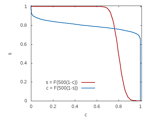
Figure 1. Example with more than one fixed point

Despite the above example, as we will see in the next section, in none of the real world or randomly generated instances we have tried we have been able to discover more than one solution.

4. Experiments

In this section, we present the results of experiments showing that on real and generated data, the algorithm presented in the last section converges quickly and to the same point, independent of the starting configuration. We also show that the computed scores are reasonable quantifications of celebritiness and spamminess in the social networks. This is done with randomly generated data sets with a random generation process that embeds the ground truth against which the output of the algorithm can be evaluated. For experimentally evaluating convergence and uniqueness properties, we use randomly generated data as well as two real-world data sets, as described in the following.

4.1. Data Sets

We use two sources of data in our experiments. The first is based on real-world data from LiveJournal. The second is randomly generated data according to a model described below. Randomly generated data allows us to compare the results of the algorithm with the “ground truth” that the model is based on. This is in contrast with the real-world data set, which is used to evaluate the convergence and uniqueness properties of the SCRank algorithm. As we show, manually skimming the results on this data suggests that the outputs are reasonable, but we do not have quantifiable ground truth.

In the rest of this section, we describe the random generation process and basic information about our real-world data set.

The random generation process

We use the following method to generate a random directed graph $G$ that will be used as a test case for our algorithm: There are $N$ nodes in the graph, out of which two disjoint sets $C$ and $S$ are designated as the set of celebrities and spammers. We then use a graph generation method such as Erdős-Rényi or preferential attachment to generate an undirected graph $H$ with the vertex set $V(G)$. The edges of this graph represent real friendship relationships among individuals. For each such edge $uv$ in $H$, with probability $1-p$ we add both directed edges $uv$ and $vu$ to $G$. With probability $p$, we add one of these two edges picked at random. This represent the fact that even among the edges corresponding to mutual friendship, some are not reciprocated. In addition to these edges, we add random directed edges from $S$ to $V(G)$ and from $V(G)$ to $C$. We underscore that this models spammers indiscriminately linking to some subset of all nodes, including possibly celebrities and other spammers, and the converse for inbound links to celebrities. For generating these edges, we use a simple model of independent coin flips: for each pair $(u,v)$ where $u\in S$ and $v\in V(G)$, we add $(u,v)$ independently with probability $p_{s}$. Similarly, for each $(u,v)$ where $u\in V(G)$ and $v\in C$, we add this edge independently with probability $p_{c}$. There is no other edge in the graph $G$.

The parameters of the model are as follows: $N$, $|C|$, $|S|$, $p$, $p_{c}$, $p_{s}$, and the parameters of the generation model for the graph $H$. The algorithm is successful if it gives high $c_{v}$ scores to nodes in $C$ (and low $c_{v}$ to nodes in $V(G)\setminus C$) and high $s_{v}$ scores to nodes in $S$ (and low $s_{v}$ to nodes in $V(G)\setminus S$).

For the experimental results we present in this paper, we have picked the following set parameters: $N=2000000$, $|C|=1000$, $|S|=5000$, $p=0.2$, $p_{c}=p_{s}=0.00025$, and the graph $H$ is a random graph with expected degree distribution that is a power law with exponent $0.5$. The average degree in $H$ is 100. These choices are mostly based on our intuition for typical numbers on a social network. We have also tried the experiments on several other sets of parameters, and did not observe any significant change in our conclusions.

LiveJournal Data Set

Each node in this data set is a LiveJournal profile, and edges correspond to friendship relationships declared on the profiles. This data set is crawled, and contains more than 4.8 million vertices and 660 million edges. LiveJournal users may choose to disallow crawling of their metadata via the robots.txt mechanism. Any user who did so was not included in the crawl, with all edges to and from this user removed from the data set.

4.2. Convergence speed

Let $\mathbf{c}$ and $\mathbf{s}$ denote the vector of $c_{v}$’s and $s_{v}$’s, respectively. We can compute the $\ell_{1}$ distance between the vector $\mathbf{c}$ computed at the end of iteration $t$, and the one computed at the end of iteration $t+1$ (and similarly for $\mathbf{s}$). When both of these values reach zero, it means that the algorithm has converged to a solution. Therefore, we can use these values as a measure of the convergence of the algorithm. We plot these values as a function of $t$ for different data sets and for different initializations of the scores, to see if and how the initialization affects convergence speed. The results (in log scale) for the three data sets are presented in Figure 2.

The initializations labelled init 0, init 1, and init 0.5 correspond to initializing all scores to zero, all scores to one, and all scores to $0.5$. We also tried initializing each score to a random number picked uniformly from $[0,1]$; this initialization produced results that were essentially indistinguishable from init 0.5 in all data sets. As can be seen in the plots, different initializations do not differ significantly in terms of their convergence rate, although init 0.5 often performs marginally better. In all cases, the convergence seems to be exponentially fast (i.e., the log-scale plot has an almost constant negative slope)

4.3. Uniqueness of the solution

To test whether the scores converge to a single point independent of the starting point, we plot the $l_{1}$ distance between the vector computed by our algorithm starting from different initializations. In particular, we measure the difference between init 0 and init 1, and between init 0 and init 0.5. The graphs, plotted as functions of $t$ in the log scale, are shown in Figure 3 for the LiveJournal and randomly generated data sets.

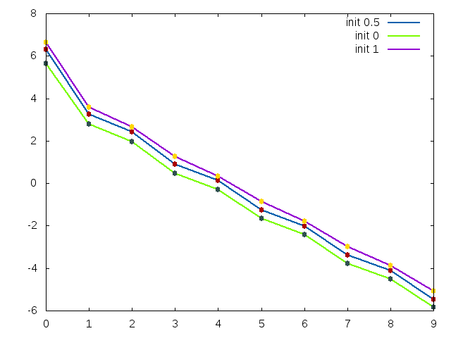
(a) LJ celebrity score

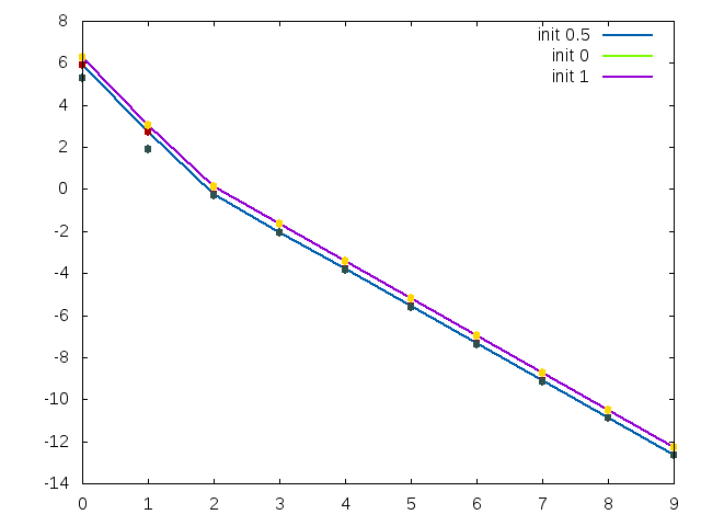
(b) Synthetic graph celebrity score

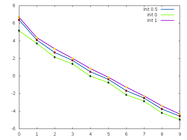
(c) LJ spammer score

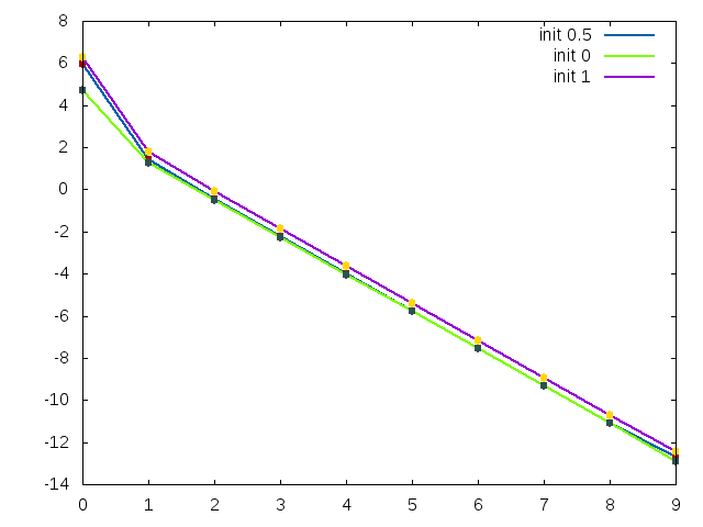
(d) Synthetic graph spammer score

Figure 2. Log-scale $l_{1}$ change in scores for LiveJournal and synthetic data, as a function of time

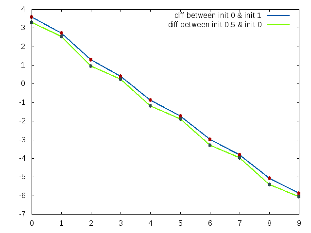
(a) LJ: celebrity scores

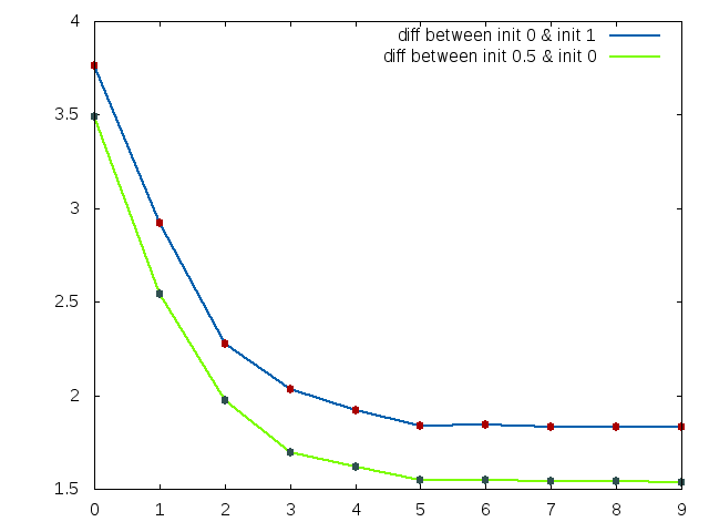
(b) Synthetic graph: celebrity scores

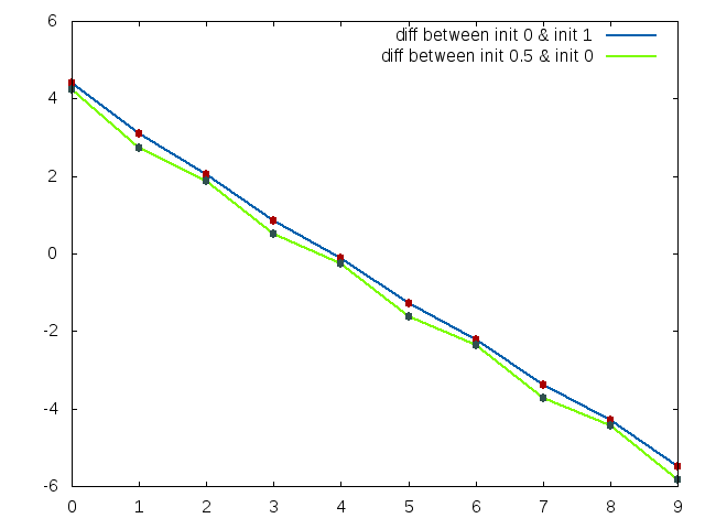
(c) LJ: spammer scores

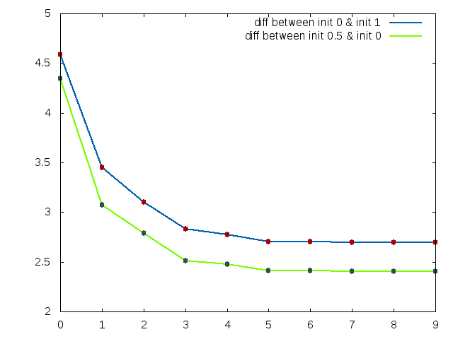
(d) Synthetic graph: spammer scores

Figure 3. Log of $l_{1}$ difference between scores computed with different initializations, as a function of time

As these graphs show, on the real-world data set after less than $10$ rounds, the solutions computed with different initializations are virtually identical. In randomly generated instances, even though the distance between the solutions decrease by about two orders of magnitude in the first five iterations, they do not converge to zero. This indicates that randomly generated instances probably contains small pockets of nodes with non-unique solutions.

4.4. Solution quality

In this section, we argue that SCRank can recover a significant portion of celebrities and spammers. To show this experimentally, we use randomly generated graphs with the sets $C$ and $S$ in the random generation process as the hidden ground truth. The algorithm is successful if it assigns high celebrity scores to nodes in $C$ and high spammer score to nodes in $S$. Figure 4 shows the distribution of celebrity and spammer scores, comparing, respectively, all vertices versus vertices in $C$; and all vertices versus vertices in $S$. The score distributions on these synthetic inputs are almost completely bimodal, with both celebrity and spammer scores of generic vertices being strongly concentrated around zero. To better observe the difference between the two distributions, we also show plots of the distribution densities with logarithmic $y$-axes.

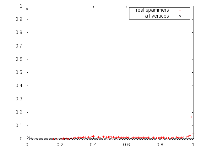
(a) Linear-scale spammer scores

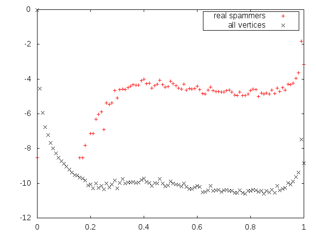
(b) Log-scale spammer scores

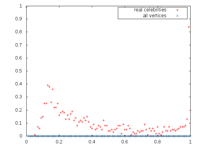
(c) Linear-scale celebrity scores

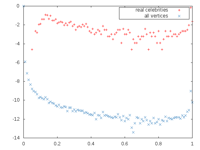
(d) Log-scale celebrity scores

Figure 4. Score distributions (p.d.f.)

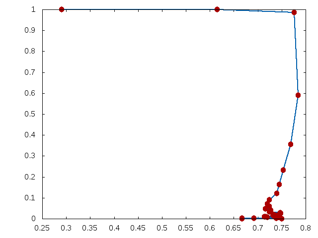
Figure 5. Precision-recall graph for the detection of spammers in a randomly generated data set.

We can also study the precision-recall tradeoff of the output of the algorithm. We plot the precision of the algorithm (which we define as the percentage of users with celebrity/spammer score more than $0.5$ who are in $C$/$S$, respectively) against recall (defined as the percentage of nodes in $C$/$S$ for which we compute a celebrity or spammer score, respectively, of more than $0.5$). By adjusting the parameters of the model, we get a tradeoff between precision and recall that is plotted in Figure 5.

5. Generalization

The potential function argument used in Section 3 to guarantee SCRank’s convergence can be generalized to a much broader class of iterative algorithms, which we expect will be of independent interest. In particular, we will show that the same argument applies to any iteration that simulates best-response dynamics in a game where players have bounded real-valued strategies, and whose utilities are strictly monotic, continuously differentiable per-variable functions which depend only on a linear combination of the others’ strategies, with symmetric linear combination weights.

Before we define this formally, let us observe how this describes the SCRank algorithm. SCRank uses $2n$ variables — two “players” per SCRank agent. The convergence argument can be rephrased to ignore the fact the variables are arranged in pairs in the original setup. The updates in lines 6–11 of the algorithm are equivalent to the $c_{i}$ players making best-response moves one at a time, then the $s_{i}$ players taking their turns. The utility/update functions for the $c_{v}$s and $s_{u}$s both depend only on a linear combination of other variables: $F_{c_{v}}(L=\sum_{u|(u,v)\in A}-s_{u})=F_{c}(\operatorname{indeg}v+L)$, and similarly for $F_{s_{u}}$. For every $(u,v)\in A$, $c_{v}$’s update function input will include $s_{u}$ with weight $-1$, and $s_{u}$’s update function input will include $c_{v}$ with weight $-1$. This meets the “symmetricity” condition — that the matrix $W$ of variable weights in the update function inputs must be symmetric. In SCRank, $W_{c_{v}s_{u}}=W_{s_{u}c_{v}}=-1$, and is 0 elsewhere.

Formally, we define a general Monotonic Üpdate on Symmetric Linear combinations Iteration (MÜSLI) system as:

• Real-valued variables $x_{1},\ldots,x_{n}$ with $x_{i}\in[a_{i},b_{i}]$

• A symmetric weight matrix $W$ with 0s on the diagonal.

• For each variable, a strictly increasing, continously differentiable update function $F_{i}:\mathbb{R}\to\mathbb{R}$ which takes as input only $(Wx)_{i}$, the linear combination of the $x_{i}$s weighted by $W$’s $i$th row. $F_{i}$ must preserve the bounds on $x_{i}$, i.e. $a_{i}\leq F_{i}((W\vec{x})_{i})\leq b_{i}$ whenever $x_{j}\in[a_{j},b_{j}]$)

• An activation sequence $A:\mathbb{Z}_{\geq 0}\to\{1,\ldots,n\}$ determining, for each iteration $t\geq 0$, the unique variable $x_{A(t)}$ that gets updated to $F_{A(t)}((Wx)_{A(t)})$.

The proof of Theorem 3.3 generalizes to show:

Theorem 5.1.

The state of a MÜSLI system, $\vec{x}$, converges to a fixed point under its iteration.

Proof.

The argument is very similar, relying just on a generalization of the potential function. As above, the strictly increasing, continuously differentiable $F_{i}$s have well-defined strictly increasing inverses $F_{i}^{-1}$, which lets us define $G_{i}(z)$ and the potential function $P(\vec{x})$ as:

$$G_{i}(z) =\int_{0}^{z}F_{i}^{-1}(t)dt\quad;\quad P(\vec{x})=\sum_{i}G_{i}(x_{i})-\frac{1}{2}\vec{x}^{T}W\vec{x}$$

This yields the partials:

$$\frac{\partial P}{\partial x_{i}}=-(W\vec{x})_{i}+F_{i}^{-1}(x_{i})$$

.

For $x^{*}_{i}=F_{i}((W\vec{x})_{i})$, this is zero, and, since $W_{ii}=0$, the first term is constant relative to $x_{i}$, and the monotonicity of $F_{i}^{-1}$ guarantees that updating $x_{i}$ to $x^{*}_{i}$ can’t increase $P(\vec{x})$.

As before, $0<\frac{dF_{i}(t)}{dt}\leq\alpha_{i}$ for some $\alpha_{i}$, and $\frac{dF^{-1}_{i}(t)}{dt}\geq 1/\alpha_{i}$. An iteration that starts at state $x^{\mathrm{old}}$ and updates $x_{i}$ from $x^{\mathrm{old}}_{i}$ to, WLOG, a lower value $x^{*}_{i}<x^{\mathrm{old}}_{i}$, changing it by $x^{\mathrm{old}}_{i}-x^{*}_{i}\geq\varepsilon$, will have, for all $t\in[x^{*}_{i},x^{\mathrm{old}}_{i}]$:

$$F^{-1}_{i}(t) >F^{-1}_{i}(x^{*}_{i})+(t-x^{*}_{i})/\alpha_{i}$$

$$=(Wx^{\mathrm{old}})_{i}+(t-x^{*}_{i})/\alpha_{i}$$

$$\frac{\partial P}{\partial x_{i}}(x^{\mathrm{old}}_{-i},t) \geq(t-x^{*}_{i})/\alpha_{i}$$

$$P(x^{\mathrm{old}})-P(x^{\mathrm{old}}_{-i},x^{*}_{i}) \geq\int_{x^{\mathrm{old}}_{i}}^{x^{*}_{i}}\frac{t-x^{*}_{i}}{\alpha_{i}}dt\geq\frac{\varepsilon^{2}}{2\alpha_{i}}$$

Since $\vec{x}$ remains within the compact set defined by $x_{i}\in[a_{i},b_{i}]$, $P(\vec{x})$ is bounded, and, since it decreases at each step of the iteration, there is, by the same argument as above, for any $\delta>0$, a step $k^{*}$ such that the update won’t change $x_{i}$ by more than $\sqrt{2\alpha_{i}\delta}$. ∎

Note that the proof doesn’t even require that each variable be “activated” infinitely often, but we expect most practical uses of this result will require that each $x_{i}$ be updated infinitely often for convergence to a relevant value, or more often than some threshold for stronger convergence bounds.

To demonstrate the breadth of these systems, we now give a couple of examples.

5.1. Example: Graph connectivity

As a trivial example of another algorithmic task solvable via a MÜSLI best-response iteration, consider the question of (undirected) graph reachability. If the graph’s adjacency matrix is used as weights, with nodes as players, using starting state 0 for all players except the origin, iterating updates of sigmoid $F_{i}(\sum_{N(i)}x_{i})$ that approximates a step function at $x=1$ will clearly converge rapidly to a state where all nodes reachable from the origin are $1$.

5.2. Example: Influence games

In SCRank and the above example, MÜSLI systems are used as algorithms to compute a fixed point of interest. We note that the one-at-a-time update dynamics and the $W_{ii}=0$ constraint mean that MÜSLI iterations can also be interpreted as classical best-response dynamics in games, immediately yielding:

Corollary 5.2.

A game whose best-response dynamics form a MÜSLI system (i.e. an $n$-player game with bounded real-valued strategies and strictly increasing, continuously differentiable best-response functions that depend only on a linear combination of the other players, with symmetric weights) is a potential game (potentialgames, ), with the above potential function, and is guaranteed to converge.

This class of games is fairly broad, including, for instance:

The party affiliation game. In the well-studied party affiliation game (FPT04, ), agents pick “political parties” $-1$ and $1$ based on the weighted sum of their friends’ and enemies’ affiliations: a player tries to be in the same party as her friends and in a different party than her enemies. Allowing fractional strategies and softening the best-response function from the original step function $F_{i}(\vec{x})=\operatorname{sgn}\sum_{j}x_{i}x_{j}w_{ij}$ to a sigmoid that approximates it produces a game whose best-response dynamics are a MÜSLI system. The above argument guarantees a potential function and convergence. We note that this is quite natural, since our potential function argument is an extension of the max cut game potential argument that underlies the analysis of the party affiliation game.

The symmetrical technology diffusion game. Consider a social network where agents are deciding, e.g., between 2 technologies with a network effect such as cellular providers where a user benefits from having more friends use the same technology. In the US cellular market, this corresponds to free phone calls to people on the same network, and heavy charges for calls to people on another network beyond a fixed monthly limit. Let weight $W_{ij}$ indicate how many minutes $i$ and $j$ expect to talk on the phone per month, $0$ and $1$ represent the provider choices, and $\vec{x}\in[0,1]^{n}$ be the current fractional provider choices, optionally considered as probabilities. A natural best-response function for $i$ is to use $(W\vec{x})_{i}$, the expected number of minutes she will spend talking to people using provider 1 (assuming minutes and provider choices are independent), as an input to a sigmoid that is a soft step function at or near the maximum number of free calling minutes for users of provider 0 when calling users of provider 1. Assuming all phone calls are 2-way, the best-response dynamics constitute a MÜSLI system, immediately demonstrating that the game is a potential game and guaranteeing convergence.

6. Conclusion

In this paper, we presented a framework for iterative algorithms for giving scores to nodes defined recursively in terms of the scores of their neighbors, with a focus with one application in which such a recursive definition comes quite naturally: computing celebrity and spammer scores on a directed social network. We theoretically proved that under a mild symmetry and monotonicity assumption, there is a potential function that decreases in every iteration of the iterative algorithm, and therefore, the iterative algorithm always converges to an approximate equilibrium. In the case of celebrity/spammer scoring, we experimentally showed that this convergence is extremely fast, the convergence point is unique, and when applied on randomly generated data with a built-in ground truth, it provides a good approximation to the ground truth.

In addition to the obvious application of finding celebrities and link-spammers in online directed social networks, we believe that our potential function framework has the potential to be quite useful in theoretical analysis of iterative algorithms on social networks. Iterative algorithms such as belief propagation are notoriously hard to analyze theoretically, despite widespread practical use.

The obvious open directions are to find other applications or generalizations of our framework, or prove a theoretical bound on the convergence speed of the algorithm that is close to the practical observation.

References

- (1) F. Benevenuto, T. Rodrigues, V. Almeida, J. Almeida, and M. Gonçalves. Detecting spammers and content promoters in online video social networks. In Proc. of SIGIR, pages 620–627. ACM, 2009.
- (2) P. Bonacich. Power and centrality: a family of measures. Amer. J. Sociology, 92:1170–1182, 1987.
- (3) P. Boutin. What’s “follow spam” on Twitter? http://gawker.com/5036236/ whats-follow-spam-on-twitter, August 12, 2008.
- (4) G. Christodoulou, V. S. Mirrokni, and A. Sidiropoulos. Convergence and approximation in potential games. In STACS 2006, volume 3884 of Lecture Notes in Computer Science, pages 349–360. 2006.
- (5) A. Fabrikant, C. H. Papadimitriou, and K. Talwar. The complexity of pure Nash equilibria. In Proc. of STOC, pages 604–612, 2004.
- (6) A. Farahat, T. LoFaro, J. C. Miller, G. Rae, and L. A. Ward. Authority rankings from hits, pagerank, and salsa: Existence, uniqueness, and effect of initialization. SIAM Journal on Scientific Computing, 27(4):1181–1201, 2006.
- (7) L. Freemann. A set of measures of centrality based on betweenness. Sociometry, 40:35–41, 1977.
- (8) S. Ghosh, B. Viswanath, F. Kooti, N. K. Sharma, G. Korlam, F. Benevenuto, N. Ganguly, and K. P. Gummadi. Understanding and combating link farming in the twitter social network. In Proc. WWW, pages 61–70, 2012.
- (9) D. Kempe, J. Kleinberg, and E. Tardos. Maximizing the spread of influence through a social network. In Proc. of KDD, pages 137–146, 2003.
- (10) J. Kleinberg. Authoritative sources in a hyperlinked environment. J. ACM, 46, 1999.
- (11) D. Monderer and L. Shapley. Potential games. Games and Economic Behavior, 14:124–143, 1996.
- (12) T. O’Reilly. Goodreads vs twitter: The benefits of asymmetric follow. http://radar.oreilly.com/2009/05/ goodreads-vs-twitter-asymmetric-follow.html, May 10, 2009.
- (13) L. Page, S. Brin, R. Motwani, and T. Winograd. The PageRank citation ranking: bringing order to the web. 1999.
- (14) S. Russell, P. Norvig, and E. Davis. Artificial intelligence: a modern approach. Prentice Hall, 2010.
- (15) J. Song, S. Lee, and J. Kim. Spam filtering in twitter using sender-receiver relationship. In R. Sommer, D. Balzarotti, and G. Maier, editors, Recent Advances in Intrusion Detection, volume 6961 of LNCS, pages 301–317. 2011.
- (16) T. Upstill, N. Craswell, and D. Hawking. Predicting fame and fortune: Pagerank or indegree? In ADCS, 2003.
- (17) A. Wang. Don’t follow me: Spam detection in twitter. In Proc. SECRYPT, pages 1–10, 2010.
- (18) S. White and P. Smyth. Algorithms for estimating relative importance in networks. In Proc. of KDD, pages 266–275, 2003.
- (19) Z. Yang, C. Wilson, X. Wang, T. Gao, B. Y. Zhao, and Y. Dai. Uncovering social network sybils in the wild. In Proc. IMC, pages 259–268, 2011.