Projection-Free Online Optimization with Stochastic Gradient: From Convexity to Submodularity

Abstract

Online optimization has been a successful framework for solving large-scale problems under computational constraints and partial information. Current methods for online convex optimization require either a projection or exact gradient computation at each step, both of which can be prohibitively expensive for large-scale applications. At the same time, there is a growing trend of non-convex optimization in machine learning community and a need for online methods. Continuous DR-submodular functions, which exhibit a natural diminishing returns condition, have recently been proposed as a broad class of non-convex functions which may be efficiently optimized. Although online methods have been introduced, they suffer from similar problems. In this work, we propose Meta-Frank-Wolfe, the first online projection-free algorithm that uses stochastic gradient estimates. The algorithm relies on a careful sampling of gradients in each round and achieves the optimal $O(\sqrt{T})$ adversarial regret bounds for convex and continuous submodular optimization. We also propose One-Shot Frank-Wolfe, a simpler algorithm which requires only a single stochastic gradient estimate in each round and achieves an $O(T^{2/3})$ stochastic regret bound for convex and continuous submodular optimization. We apply our methods to develop a novel “lifting” framework for the online discrete submodular maximization and also see that they outperform current state-of-the-art techniques on various experiments.

1 Introduction

As the amount of collected data becomes massive in both size and complexity, algorithm designers are faced with unprecedented challenges in statistics, machine learning, and control. In the past decade, online optimization has provided a successful computational framework for tackling a wide variety of challenging problems, ranging from non-parametric regression to portfolio management (Calandriello et al., 2017; Agarwal et al., 2006). In online optimization, a large or complex optimization problem is broken down into a sequence of smaller optimization problems, each of which must be solved with limited information. This framework captures many real-world scenarios in which standard optimization theory does not apply. For instance, a machine learning application cannot feasibly process terabytes of data at a single time; rather, subsets of data may be handled in a sequential fashion. Another example is when the true objective function is the expectation of an unknown distribution of functions, and may only be accessible via samples, as is the case for problems in online learning and control theory (Xiao, 2010; Wang & Boyd, 2008).

Online convex optimization, a branch of online optimization that considers sequentially minimizing convex functions, has proved particularly useful for statistical and machine learning applications. Online convex optimization has enjoyed much success in these areas because most offline machine learning techniques utilize the existing theory of convex optimization. As in the offline setting, gradient methods are a popular class of algorithms for online convex optimization due to their simplicity; however, they require projections onto the constraint set, which involve solving a quadratic program in the general case. These projections are infeasible for large scale applications with complicated constraints such as matrix completion, network routing problems, and maximum matchings. Online projection-free methods have been proposed and are much more efficient , replacing a projection onto the constraint set with a linear optimization over the constraint set at each iteration (Hazan & Kale, 2012; Garber & Hazan, 2013). However, these projection-free methods require exact gradient computations, which may be prohibitively expensive for even moderately sized data sets and intractable when a closed form does not exist. Thus, there is a huge need for online convex optimization routines that are projection-free and also robust to stochastic gradient estimates.

While convex programs may be efficiently solved (at least in theory), there is a growing number of non-convex problems arising in machine learning and statistics. Notable examples include nonnegative principle component analysis, low-rank matrix recovery, sigmoid loss functions for binary classification, and the training of deep neural networks, to name a few. Understanding which types of non-convex functions may be efficiently optimized and developing techniques for doing so is a pressing research question for both theory and practice. Recently, continuous DR-submodular functions have been proposed as a broad class of non-convex functions which admit efficient approximate maximization routines, even though exact maximization is NP-Hard (Bian et al., 2017). These functions capture many real-life applications, such as optimal experiment design, non-definite quadratic programming, coverage and diversity functions, and continuous relaxation of discrete submodular functions. Recent works (Chen et al., 2018) have proposed methods for online continuous DR-submodular optimization; however, these too require either expensive projections or exact gradient computations.

Our contributions

In this paper, we present a suite of projection-free algorithms for online optimization that use stochastic estimates of the gradient and leverage the averaging technique (Mokhtari et al., 2018a, b) to reduce their variance. This includes

• Meta-Frank-Wolfe, the first projection-free algorithm for adversarial online optimization which requires only stochastic gradient estimates. The algorithm relies on a careful sampling of gradients in each round and achieves optimal $O(\sqrt{T})$ regret and $(1-1/e)$-regret bounds for convex and submodular optimization, respectively.

• One-Shot Frank-Wolfe, a simpler projection-free algorithm for stochastic online optimization which requires only a single stochastic gradient estimate in each round. This simpler algorithm achieves $O(T^{2/3})$ regret and $(1-1/e)$-regret bounds for the convex and submodular case, respectively.

• A novel class of algorithms for online discrete submodular optimization which are based on lifting discrete functions to the continuous domain, applying our methods with an extremely efficient sampling technique, and using rounding schemes to produce a discrete solution.

Finally, to demonstrate the effectiveness of our algorithms, we tested their performance on an extensive set of experiments and measured against common baselines.

2 Related Work

The Frank-Wolfe algorithm, also known as the conditional gradient descent, was originally proposed for the offline setting in (Frank & Wolfe, 1956). The framework of online convex optimization was introduced by Zinkevich (2003), in which the online projected gradient descent was proposed and proved to achieve an $O(\sqrt{T})$ regret bound. However, the projections required for such an algorithm are too expensive for many large-scale online problems. The online conditional gradient descent was the first projection-free online algorithm, originally proposed in (Hazan & Kale, 2012). An improved conditional gradient algorithm was later designed for smooth and strongly convex optimization which achieves the optimal $O(\sqrt{T})$ adversarial regret bound (Garber & Hazan, 2013). However, both of these algorithms can perform arbitrarily poorly if supplied with stochastic gradient estimates. Lafond et al. (2015) proposed an online Frank-Wolfe variant for the any-time stochastic online setting that converges to a stationary point for non-convex expected functions . While convergence is an important property of the any-time methods, arbitrary stationary points do not yield approximation guarantees for general non-convex functions.

Johnson & Zhang (2013) introduced the variance reduction technique for accelerating stochastic gradient descent. It was independently discovered by Mahdavi et al. (2013). Allen-Zhu & Hazan (2016) applied this technique to non-convex optimization. Hazan & Luo (2016) devised a projection-free stochastic convex optimization algorithm based on this technique. Mokhtari et al. (2018a, b) proposed the first sample-efficient variance reduction technique for projection-free algorithms that does not require increasing batch sizes. Their method achieves the tight $(1-1/e)$ approximation guarantee for monotone and continuous DR-submodular functions. Although these variance reduction techniques have enjoyed success in the offline setting, they have yet to be as extensively applied in the online setting that we consider in this paper.

In the discrete domain, Streeter & Golovin (2009) studied the online maximization problem of monotone submodular set functions subject to a knapsack constraint and introduced the meta-action technique. In a celebrated work, Calinescu et al. (2011) proposed an (offline) method for maximizing monotone submodular set functions subject to a matroid constraint by working in the continuous domain via the multilinear extension, then rounding the fractional solution. By combining the meta-action and lifting techniques, Golovin et al. (2014) presented an algorithm whose $(1-1/e)$-regret is bounded by $O(\sqrt{T})$. The lifting method therein relies on an expensive sampling procedure that does not scale favorably to large applications.

Bach (2015) demonstrated connections between continuous submodular functions and convex functions in the context of minimization. Building upon the continuous greedy algorithm of (Calinescu et al., 2011), Bian et al. (2017) proposed an algorithm that achieves a $(1-1/e)$-approximation guarantee for maximizing monotone continuous DR-submodular functions subject to down-closed convex constraints. Projected gradient methods were investigated in (Hassani et al., 2017) and were shown to attain a $1/2$-approximation ratio for monotone continuous DR-submodular functions. Very recently, Chen et al. (2018) borrowed the idea of meta-action (Streeter & Golovin, 2009) and proposed several online algorithms for maximizing monotone continuous DR-submodular functions. However, each of these methods either requires an expensive projection step at each iteration or cannot handle stochastic gradient estimates.

3 Preliminaries

In this work, we are interested in optimizing two classes of functions, namely convex and continuous DR-submodular. To begin defining continuous submodular functions, we first recall the definition of a submodular set function. A real-valued set function $f:2^{\Omega}\rightarrow\mathbb{R}_{+}$ is submodular if

$$f(A)+f(B)\geq f(A\cup B)+f(A\cap B)$$

for all $A,B\subset\Omega$. The notion of submodularity has been extended to continuous domains (Wolsey, 1982; Vondrák, 2007; Bach, 2015). Consider a function $f:\mathcal{X}\rightarrow\mathbb{R}_{+}$ where the domain is of the form $\mathcal{X}=\prod_{i=1}^{n}\mathcal{X}_{i}$ and each $\mathcal{X}_{i}$ is a compact subset of $\mathbb{R}_{+}$. We say that $f$ is continuous submodular if $f$ is continuous and for all $\mathbf{x},\mathbf{y}\in\mathcal{X}$, we have

$$f(\mathbf{x})+f(\mathbf{y})\geq f(\mathbf{x}\vee\mathbf{y})+f(\mathbf{x}\wedge\mathbf{y})$$

where $\mathbf{x}\vee\mathbf{y}$ and $\mathbf{x}\wedge\mathbf{y}$ are component-wise maximum and minimum, respectively. Note that we have defined both discrete and continuous functions to be nonnegative on their respective domains. For efficient maximization, we also require that these functions satisfy a diminishing returns condition (Bian et al., 2017). We say that $f$ is continuous DR-submodular if $f$ is differentiable and

$$\nabla f(\mathbf{x})\geq\nabla f(\mathbf{y})$$

for all $\mathbf{x}\leq\mathbf{y}$. The main attraction of continuous DR-submodular functions is that they are concave in positive directions; that is, for all $\mathbf{x}\leq\mathbf{y}$,

$$f(\mathbf{y})\leq f(\mathbf{x})+\langle\nabla f(\mathbf{x}),\mathbf{y}-\mathbf{x}\rangle$$

(Calinescu et al., 2011; Bian et al., 2017). A function $f$ is monotone if $f(\mathbf{x})\leq f(\mathbf{y})$ for all $\mathbf{x}\leq\mathbf{y}$. A function $f$ is $L$-smooth if $\|\nabla f(\mathbf{x})-\nabla f(\mathbf{y})\|\leq L\|\mathbf{x}-\mathbf{y}\|$ for all $\mathbf{x},\mathbf{y}$.

We now provide a brief introduction to online optimization, referring the interested reader to the excellent survey of (Hazan et al., 2016). In the online setting, a player seeks to iteratively optimize a sequence of functions $f_{1},\dots f_{T}$ over $T$ rounds. In each round, a player must first choose a point $\mathbf{x}_{t}$ from the constraint set $\mathcal{K}$. After playing $\mathbf{x}_{t}$, the value of $f_{t}(\mathbf{x}_{t})$ is revealed to the player, along with access to the gradient $\nabla f$. Although the player does not know the function $f_{t}$ while choosing $\mathbf{x}_{t}$, they may use information of previously seen functions to guide their choice. The situation where an arbitrary sequence of functions $f_{1},\dots,f_{T}$ is presented is known as the adversarial online setting. In the adversarial setting, the goal of the player is to minimize adversarial regret, which is defined as

$$\mathcal{R}_{T}\triangleq\sum_{t=1}^{T}f_{t}(\mathbf{x}_{t})-\inf_{\mathbf{x}\in\mathcal{K}}\sum_{t=1}^{T}f_{t}(\mathbf{x})$$

for minimization problems and analogously defined for maximization problems. Intuitively, a player’s regret is low if the accumulated value of their actions over the $T$ rounds is close to that of the single best action in hindsight. Indeed, this is a natural framework for data-intensive applications where the entire data may not fit onto a single disk and thus needs to be processed in $T$ batches. The algorithm designer would like to devise a scheme to process the $T$ batches separately in a way that is competitive with the best single disk solution.

A slightly different formulation known as stochastic online setting is when the functions are chosen $i.i.d.$ from some unknown distribution $f_{t}\sim\mathcal{D}$. In this case, the player seeks to minimize stochastic regret, which is defined as

$$\mathcal{SR}_{T}\triangleq\sum_{t=1}^{T}f(\mathbf{x}_{t})-T\cdot\inf_{\mathbf{x}\in\mathcal{K}}f(\mathbf{x})$$

where $f(\mathbf{x})=\mathbb{E}_{f_{t}\sim\mathcal{D}}[f_{t}(\mathbf{x})]$ denotes the expected function. This is a natural framework for many statistical and machine learning applications, such as empirical risk minimization, where the true objective is unknown but pairs of data points and labels are sampled. While the stochastic setting appears “easier” than the adversarial setting (in the sense that any strategy for the adversarial settings applies to stochastic settings and obtains a potentially lower regret), the strategies designed for the stochastic setting may be much simpler and more computationally efficient. For both adversarial and stochastic settings, a strategy that achieves a regret that is sublinear in $T$ is considered good and $O(\sqrt{T})$ regret bounds are optimal for convex functions in both settings. Although convex programs can be efficiently solved to high accuracy, general non-convex programs cannot be efficiently exactly optimized, thus necessitating another definition of regret. The $\alpha$-regret is defined as

$$\alpha\mbox{-}\mathcal{R}_{T}\triangleq\alpha\sup_{\mathbf{x}\in\mathcal{K}}\sum_{t=1}^{T}f_{t}(\mathbf{x})-\sum_{t=1}^{T}f_{t}(\mathbf{x}_{t})$$

for adversarial maximization problems, and may be analogously extended to other scenarios. Intuitively, $\alpha$-regret compares a player’s actions with the best $\alpha$-approximation to the optimal solution in hindsight. This is appropriate when the objective functions do not admit efficient optimization routines, but do admit constant-factor approximations, as is the case with continuous DR-submodular functions.

Nearly all optimization methods for both offline and online settings use first order information of the objective function; however, exact gradient computations can be costly, especially when the objective function is only readily expressed as a large sum of individual functions or is itself an expectation over an unknown distribution. In this case, stochastic estimates are usually much more computationally efficient to obtain via sampling or simulation. In this work, we assume that once a function $f_{t}$ is revealed, the player gains oracle access to unbiased stochastic estimates of the gradient, rather than the exact gradient. More precisely, the player may query the oracle to obtain a random linear function $\tilde{\nabla}f(x)$ such that $\mathbb{E}[\nabla f(x)-\tilde{\nabla}f(x)]=0$ for all $x$. This computational model captures commonly used mini-batch methods for estimating gradients, among other examples. In this work, we make a few main assumptions that allow our algorithms to be analyzed.

Assumption 1.

The constraint set $\mathcal{K}$ is convex and compact, with diameter $D=\sup_{\mathbf{x},\mathbf{y}\in\mathcal{K}}\|\mathbf{x}-\mathbf{y}\|$ and radius $R=\sup_{\mathbf{x}\in\mathcal{K}}\|\mathbf{x}\|$.

Assumption 2.

In the adversarial setting, each function $f_{t}$ is $L$-smooth and in the stochastic setting, the expected function $f$ is $L$-smooth.

Assumption 3.

In the adversarial setting, the gradient oracle is unbiased $\mathbb{E}[\nabla f_{t}(\mathbf{x})-\tilde{\nabla}f_{t}(\mathbf{x})]=0$ and has a bounded variance $\mathbb{E}[\|\nabla f_{t}(\mathbf{x})-\tilde{\nabla}f_{t}(\mathbf{x})\|^{2}]\leq\sigma^{2}$ for all points $\mathbf{x}$ and functions $f_{t}$. In the stochastic setting, the gradient oracle is unbiased $\mathbb{E}[\nabla f(\mathbf{x})-\tilde{\nabla}f_{t}(\mathbf{x})]=0$ and has a bounded variance $\mathbb{E}[\|\nabla f(\mathbf{x})-\tilde{\nabla}f_{t}(\mathbf{x})\|^{2}]\leq\sigma^{2}$ for all points $\mathbf{x}$ and functions $f_{t}$.

We remark that in the stochastic setting and under mild regularity conditions, unbiasedness of the gradients $\mathbb{E}[\nabla f_{t}(\mathbf{x})-\tilde{\nabla}f_{t}(\mathbf{x})]=0$ implies unbiasedness $\mathbb{E}[\nabla f(\mathbf{x})-\tilde{\nabla}f_{t}(\mathbf{x})]=0$ in Assumption 3 because $f(\mathbf{x})=\mathbb{E}_{f_{t}\sim\mathcal{D}}[f_{t}(\mathbf{x})]$ Moreover, upper bounds on the variance terms $\mathbb{E}[\|\nabla f(\mathbf{x})-\nabla f_{t}(\mathbf{x})\|^{2}]\leq\sigma_{a}^{2}$ and $\mathbb{E}[\|\nabla f_{t}(\mathbf{x})-\tilde{\nabla}f_{t}(\mathbf{x})\|^{2}]\leq\sigma_{b}^{2}$ yield a variance bound of $\mathbb{E}[\|\nabla f(\mathbf{x})-\tilde{\nabla}f_{t}(\mathbf{x})\|^{2}]\leq\sigma_{a}^{2}+\sigma_{b}^{2}$ , by the triangle inequality.

4 Main Results

We now present two algorithms for online optimization of convex and continuous DR-submodular functions in the adversarial and stochastic settings. Unlike previous work, these methods are projection-free and require only stochastic estimates of the gradients, rather than exact gradient computations. In both algorithms, the main computational primitive is linear optimization over a compact convex set. In addition, we remark that both algorithms can be converted into an anytime algorithm that does not require the knowledge of the horizon $T$ via the doubling trick; see Section 2.3.1 of (Shalev-Shwartz et al., 2012).

4.1 Adversarial Online Setting

Algorithm 1 combines the recent variance reduction technique of (Mokhtari et al., 2018a) along with the use of online linear optimization oracles to minimize the regret in each round. An online linear optimization oracle is an instance of an online linear optimization (minimization/maximization in the convex/DR-submodular setting, respectively) algorithm that optimizes linear objectives in a sequential manner. Both the variance reduction in the stochastic gradient estimates and the online linear oracles are crucial in the algorithm, as just one technique is not enough to get sublinear regret bounds in the adversarial setting. At a high level, our algorithm produces iterates $x_{t}$ by running $K$ steps of a Frank-Wolfe procedure, using an average of previous gradient estimates and linear online optimization oracles in place of exact optimization of the true gradient. After a point $x_{t}$ is played in round $t$, our algorithm queries the gradient oracle $\tilde{\nabla}f_{t}$ at $K$ points. Then, the gradient estimates are averaged with those from previous rounds and fed as objective functions into $K$ linear online optimization oracles. The $K$ points chosen by the oracles are used as iterates in a full $K$-step Frank-Wolfe subroutine to obtain the next point $x_{t+1}$. A formal description is provided in Algorithm 1.

0:  convex set $\mathcal{K}$, time horizon $T$, linear optimization oracles $\mathcal{E}^{(1)}\dots\mathcal{E}^{(K)}$, step sizes $\rho_{k}\in(0,1)$ and $\eta_{k}\in(0,1)$, and initial point $\mathbf{x}_{1}$

0:  $\{\mathbf{x}_{t}:1\leq t\leq T\}$

1:  Initialize online linear optimization oracles $\mathcal{E}^{(1)}\ldots\mathcal{E}^{(K)}$

2:  Initialize $\mathbf{d}_{t}^{(0)}=0$ and $\mathbf{x}_{t}^{(1)}=\mathbf{x}_{1}$

3:  for $t\leftarrow 1,2,3,\ldots,T$ do

4:     $\mathbf{v}_{t}^{(k)}\leftarrow$ output of oracle $\mathcal{E}^{(k)}$ in round $t-1$

5:     $\mathbf{x}_{t}^{(k+1)}\leftarrow update(\mathbf{x}_{t}^{(k)},\mathbf{v}_{t}^{(k)},\eta_{k})$ for $k=1\dots K$

6:     Play $\mathbf{x}_{t}=\mathbf{x}_{t}^{(K+1)}$, then obtain value $f_{t}(\mathbf{x}_{t})$ and unbiased oracle access to $\nabla f_{t}$

7:     $\mathbf{d}_{t}^{(k)}\leftarrow(1-\rho_{k})\mathbf{d}_{t}^{(k-1)}+\rho_{k}\tilde{\nabla}f_{t}(\mathbf{x}_{t}^{(k)})$ for $k=1\ldots K$

8:     Feedback $\langle\mathbf{v}_{t}^{(k)},\mathbf{d}_{t}^{(k)}\rangle$ to $\mathcal{E}^{(k)}$ for $k=1\dots K$

9:  end for

Algorithm 1 Meta-Frank-Wolfe

There are only a few differences in Algorithm 1 for convex and submodular optimization. First, the online oracles should be minimizing in the case of convex optimization and maximizing in the case of submodular optimization. Second, the initial point $\mathbf{x}_{1}$ may be any point in $\mathcal{K}$ for convex problems but should be set to $0$ for submodular problems (even if $\mathcal{K}$ is not down-closed). Finally, the update rule is

$$\mathbf{x}_{t}^{(k+1)}\leftarrow(1-\eta_{k})\mathbf{x}_{t}^{(k)}+\eta_{k}\mathbf{v}_{t}^{(k)}$$

for convex problems and

$$\mathbf{x}_{t}^{(k+1)}\leftarrow\mathbf{x}_{t}^{(k)}+\eta_{k}\mathbf{v}_{t}^{(k)}$$

for submodular problems. We now provide a formal regret bound.

Theorem 1 (Proof in Appendices C and B).

Suppose Assumptions 1 - 3 hold, the online linear optimization oracles have regret at most $\mathcal{R}_{T}^{\mathcal{E}}$, and the averaging parameters are chosen as $\rho_{k}=\frac{2}{(k+3)^{2/3}}$. Then for convex functions $f_{1},\dots,f_{T}$ and step sizes $\eta_{k}=\frac{1}{k+3}$, the adversarial regret of Algorithm 1 is at most

$$\frac{4TDQ^{1/2}}{K^{1/3}}+\frac{4T}{K}\left(M+\frac{LD^{2}}{3}\log(K+1)\right)+\frac{4}{3}\mathcal{R}_{T}^{\mathcal{E}}$$

in expectation, where $M=\max_{1\leq t\leq T}\left[f_{t}(\mathbf{x}_{1})-f_{t}(\mathbf{x}^{*})\right]$ and $Q\triangleq\max\{4^{2/3}\max_{1\leq t\leq T}\|\nabla f_{t}(\mathbf{x}_{1})\|^{2},4\sigma^{2}+3(LD)^{2}/2\}$. For monotone continuous DR-submodular functions $f_{1},\dots,f_{T}$ and step sizes $\eta_{k}=\frac{1}{K}$, the adversarial $(1-1/e)$-regret of Algorithm 1 is at most

$$\frac{3TDQ^{1/2}}{2K^{1/3}}+\frac{LD^{2}T}{2K}+\mathcal{R}_{T}^{\mathcal{E}}$$

in expectation, where $Q\triangleq\max\{\max_{1\leq t\leq T}\lVert\nabla f_{t}(\mathbf{x}_{1})\rVert^{2}4^{2/3},4\sigma^{2}+6L^{2}R^{2}\}$.

From Theorem 1, we observe that by setting $K=T^{3/2}$ and choosing a projection-free online linear optimization oracle with $\mathcal{R}_{T}^{\mathcal{E}}=O(\sqrt{T})$, such as Follow the Perturbed Leader (Cohen & Hazan, 2015), both regrets are bounded above by $O(\sqrt{T})$. We remark that the expectation in Theorem 1 is with respect to the stochastic gradient estimates.

4.2 Stochastic Online Setting

In the stochastic online setting, where functions are sampled i.i.d. $f_{t}\sim\mathcal{D}$, we can develop much simpler algorithms that still achieve sublinear regret. Algorithm 2 works without instantiating any online linear optimization oracles and requires only a single stochastic estimate of the gradient at each round. Indeed, because the functions are not arbitrarily chosen, variance reduction along with one Frank-Wolfe step suffices to achieve a sublinear regret bound.

0:  convex set $\mathcal{K}$, time horizon $T$, step sizes $\rho_{t}\in(0,1)$ and $\eta_{t}\in(0,1)$, and initial point $\mathbf{x}_{1}$

0:  $\{\mathbf{x}_{t}:1\leq t\leq T\}$

1:  $\mathbf{d}_{0}\leftarrow 0$

2:  for $t\leftarrow 1,2,3,\ldots,T$ do

3:     Play $\mathbf{x}_{t}$, then obtain value $f_{t}(\mathbf{x}_{t})$ and unbiased oracle access to $\nabla f_{t}$

4:     $\mathbf{d}_{t}\leftarrow(1-\rho_{t})\mathbf{d}_{t-1}+\rho_{t}\tilde{\nabla}f_{t}(\mathbf{x}_{t})$

5:     $\mathbf{v}_{t}\leftarrow\operatorname*{arg\,max}_{\mathbf{v}\in\mathcal{K}}\langle\mathbf{d}_{t},\mathbf{v}\rangle$

6:     $\mathbf{x}_{t+1}\leftarrow update(\mathbf{x}_{t},\mathbf{v}_{t},\eta_{t})$

7:  end for

Algorithm 2 One-Shot Frank-Wolfe

The differences in Algorithm 2 for convex and submodular optimization are similar to those in Algorithm 1. Namely, the update rules are the same and the initial point $\mathbf{x}_{1}$ may be arbitrarily chosen from $\mathcal{K}$ for convex optimization, and set to $0$ for submodular optimization.

Theorem 2 (Proof in Appendices E and D).

Suppose Assumptions 1 - 3 hold and the averaging parameters are chosen as $\rho_{t}=\frac{2}{(t+3)^{2/3}}$. Then for a convex expected function $f$ and step sizes $\eta_{t}=\frac{1}{t+3}$, the stochastic regret of Algorithm 1 is at most

$$4M\log(T+1)+6Q^{1/2}DT^{2/3}+\frac{4}{3}LD^{2}\log^{2}(T+3)$$

in expectation, where $M=f(\mathbf{x}_{1})-f(\mathbf{x}^{*})$ and $Q\triangleq\max\{4^{2/3}\|\nabla F(\mathbf{x}_{1})\|^{2},4\sigma^{2}+3(LD)^{2}/2\}$. For expected functions $f$ which are monotone continuous DR-submodular and step sizes $\eta_{k}=\frac{1}{K}$, the stochastic $(1-1/e)$-regret of Algorithm 2 is at most

$$(1-1/e)M+\frac{3DQ^{1/2}}{10}(3T^{2/3}+2T^{-1})+\frac{LD^{2}}{2}.$$

in expectation, where $M=f(\mathbf{x}^{*})-f(0)$ and $Q\triangleq\max\{\lVert\nabla f(0)\rVert^{2}4^{2/3},4\sigma^{2}+6L^{2}R^{2}\}$

4.3 Lifting Methods for Discrete Online Optimization

One exciting application of our online continuous DR-submodular optimization algorithms is a new approach for online discrete submodular optimization. While previous methods could only handle knapsack constraints (Streeter & Golovin, 2009) or required expensive sampling procedures (Golovin et al., 2014), our continuous methods can be applied to the discrete setting to handle general matroid constraints and computationally cheap sampling procedures.

Suppose $f_{1},\dots f_{T}$ are nonnegative monotone submodular set functions on a ground set $\Omega$ with matroid constraint $\mathcal{I}$ and $\bar{f}_{1},\dots\bar{f}_{T}$ are corresponding multi-linear extensions with matroid polytope $\mathcal{K}\subset[0,1]^{n}$. A discrete procedure that uses our continuous algorithm is as follows: at each round $t$, the online continuous algorithm produces a fractional solution $\mathbf{x}_{t}\in\mathcal{K}$, which is then rounded to a set $X_{t}\in\mathcal{I}$ and played as the discrete solution. The value $f_{t}(X_{t})$ is revealed and the player is granted access to the discrete function $f_{t}$. Then, the player supplies the continuous algorithm with a stochastic gradient estimate $\tilde{\nabla}\hat{f}_{t}$ obtained by a single function evaluation, as

$$\frac{\partial f_{t}(\mathbf{x})}{\partial x_{i}}=\mathbb{E}[f(R\cup\{i\})-f(R)],\enspace\forall i\in[n],$$ (1)

where $R$ is random subset of $[n]\setminus\{i\}$ such that for every $j\in[n]\setminus\{i\}$, the event $j\in R$ happens with an independent probability of $x_{j}$. Because a lossless rounding scheme is used, the discrete player enjoys a regret that is no worse than that of the continuous solution. Provably lossless rounding schemes include the pipage rounding (Ageev & Sviridenko, 2004; Calinescu et al., 2011) and contention resolution (Vondrák et al., 2011).

Most discrete submodular maximization algorithms that go through the multi-linear extension require a gradient estimate with high accuracy. In order to do this, they appeal to a concentration bound, which requires $O(n^{2})$ evaluations of the discrete function for independently chosen samples. In stark contrast, our algorithms can handle stochastic gradient estimates and thus require only a single function evaluation, finally making continuous methods a reality for large-scale online discrete optimization problems. The framework of the one-sampling lifting method is illustrated in Fig. 1.

Figure 1: Diagram of the one-sample lifting method

As an example, we present in Algorithm 3 how to use Meta-Frank-Wolfe as an online maximization algorithm of submodular set functions. According to Theorem 1, the $(1-1/e)$-regret of Algorithm 3 is bounded by $\frac{3TDQ^{1/2}}{K^{1/3}}+\frac{LD^{2}T}{2K}+\mathcal{R}_{T}^{\mathcal{E}}$, where $\mathcal{R}_{T}^{\mathcal{E}}$ is the regret of $\mathcal{E}^{(k)}$ up to horizon $T$. If one sets $\mathcal{E}^{(k)}$ to an online linear maximization algorithm with regret bound $O(\sqrt{T})$ and sets $K=T^{3/2}$, the $(1-1/e)$-regret is at most $O(\sqrt{T})$.

0:  matroid constraint $\mathcal{I}$, time horizon $T$, linear optimization oracles $\mathcal{E}^{(1)}\dots\mathcal{E}^{(K)}$, step sizes $\rho_{k}\in(0,1)$ and $\eta_{k}\in(0,1)$, and initial point $\mathbf{x}_{1}$

0:  $\{X_{t}:1\leq t\leq T\}$

1:  Initialize online linear optimization oracles $\mathcal{E}^{(1)}...\mathcal{E}^{(K)}$, setting the constraint set to the matroid polytope of $\mathcal{I}$

2:  Initialize $\mathbf{d}_{t}^{(0)}=0$ and $\mathbf{x}_{t}^{(1)}=\mathbf{x}_{1}$

3:  for $t\leftarrow 1,2,3,\ldots,T$ do

4:     $\mathbf{v}_{t}^{(k)}\leftarrow$ output of oracle $\mathcal{E}^{(k)}$ in round $t-1$

5:     $\mathbf{x}_{t}^{(k+1)}\leftarrow update(\mathbf{x}_{t}^{(k)},\mathbf{v}_{t}^{(k)},\eta_{k})$ for $k=1\ldots K$

6:     $\mathbf{x}_{t}\leftarrow\mathbf{x}_{t}^{(K+1)}$

7:     play $X_{t}\leftarrow round(\mathbf{x}_{t})$, obtain value $f_{t}(X_{t})$ and observe the function $f_{t}$

8:     Sample $\tilde{\nabla}\bar{f}_{t}(\mathbf{x}_{t}^{(k)})$ for $k=0,\ldots,K-1$

9:     $\mathbf{d}_{t}^{(k)}\leftarrow(1-\rho_{k})\mathbf{d}_{t}^{(k-1)}+\rho_{k}\tilde{\nabla}f_{t}(\mathbf{x}_{t}^{(k)})$ for $k=1\ldots K$

10:     Feedback $\langle\mathbf{v}_{t}^{(k)},\mathbf{d}_{t}^{(k)}\rangle$ to $\mathcal{E}^{(k)}$ for $k=1\ldots K$

11:  end for

Algorithm 3 Meta-Frank-Wolfe for online discrete submodular maximization

5 Experiment

In this section, we test our online algorithms for monotone continuous DR-submodular and convex optimization on both real-world and synthetic data sets. We find that our algorithms outperform most baselines, including projected gradient descent, when supplied with stochastic gradient estimates. All code was written in the Julia programming language and tested on a Macintosh desktop with an Intel Processor i7 with 16 GB of RAM. No parts of the code were optimized past basic Julia usage. A list of all algorithms to be compared in this section is presented below.

• Meta-Frank-Wolfe is Algorithm 1. We compare the variance-reduced meta-Frank-Wolfe algorithm and the analogue without variance reduction, denoted Meta-FW w/ VR and Meta-FW w/o VR, respectively.

• One-shot Frank-Wolfe is Algorithm 2. We compare the One-shot online Frank-Wolfe algorithm with and without variance reduction, denoted OS-FW w/ VR OS-FW w/o NVR, respectively.

• Regularized online Frank-Wolfe is referred to as the online conditional gradient algorithm in (Hazan et al., 2016). It has a regularizer term when computing the gradient. Thus we term it the regularized online Frank-Wolfe algorithm and denote it as Regularized-OFW.

• Online projected gradient ascent (OGA) follows the direction of the projected gradient. Its $1/2$-regret is at most $O(\sqrt{T})$ for online monotone continuous DR-submodular maximization if the step size is set to $\Theta(1/\sqrt{t})$ on the $t$-th iteration (Chen et al., 2018). Note that OGA is not a projection-free algorithm. In the setting of convex minimization, we use online projected gradient descent instead (denoted by OGD).

• When we perform experiments on discrete submodular maximization problems using our lifting method, we also compare the above algorithms with the Online Greedy algorithm (Streeter & Golovin, 2009).

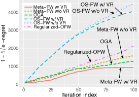
(a) Continuous facility location on Jester dataset

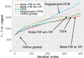
(b) Discrete facility location on Jester dataset

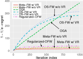
(c) News recommendation in Reuters corpus

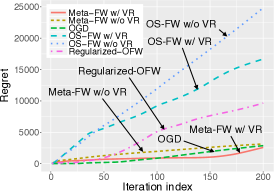
(d) Network flow

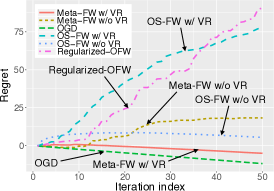
(e) Matrix completion

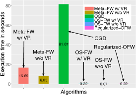
(f) Execution time of matrix completion

Figure 2: Figs. 2(a), 2(b) and 2(c) shows the $(1-1/e)$-regret of online DR-submodular maximization algorithms. In Figs. 2(a) and 2(b), we show the regret for the continuous and discrete facility location objective functions on the Jester dataset, respectively. We show the results for the online news recommendation problem in the Reuters corpus in Fig. 2(c). The results for online convex minimization are illustrated in Figs. 2(d), 2(e) and 2(f). In Fig. 2(d), we show the regret of the algorithms applied to the stochastic cost network flow problem. The results for the matrix completion problem are shown in Fig. 2(e) and the computational time is illustrated in Fig. 2(f).

5.1 Online DR-Submodular Maximization

In order to test the performance of algorithms for online maximization of monotone continuous DR-submodular functions with stochastic gradient estimates, we conducted three sets of experiments on real-world datasets. We approximate the $(1-1/e)$-regret by running an offline Frank Wolfe maximization to produce a solution that is a $(1-1/e)$ approximation to the optimum.

Joke Recommendations (Continuous)

The first set of experiments is to optimize a sequence of continuous facility location objectives on the Jester dataset (Goldberg et al., 2001). It contains ratings of 100 jokes from 73,421 users and the rating range is $[-10,10]$. We re-scale the rating range into $[0,20]$ so that all ratings are non-negative. Let $R_{uj}$ be user $u$’s rating of joke $j$. All users are splitted into disjoint batches $B_{1},B_{2},\ldots,B_{T}$, each containing $B$ users. The facility location objective is defined as $f_{t}(X)=\sum_{u\in B_{t}}\max_{j\in X}R_{uj},\enspace\forall X\subseteq[J]$, where $J=100$ is the total number of jokes and $[J]=\{1,2,3,\ldots,J\}$. Its multilinear extension is given by $\bar{f}_{t}(\mathbf{x})=\sum_{u\in B_{t}}\sum_{l=1}^{J}R_{uj_{u}^{l}}\mathbf{x}_{j_{u}^{l}}\prod_{m=1}^{l-1}(1-\mathbf{x}_{j_{u}^{m}}),\enspace\forall\mathbf{x}\in[0,1]^{J}$, where $j^{1}_{u},j^{2}_{u},\dots,j^{J}_{u}$ is a permutation of $1,2,\dots,J$ such that $R_{uj^{1}_{u}}\geq R_{uj^{2}_{u}}\geq\dots\geq R_{uj^{J}_{u}}$ (Iyer et al., 2014). In this experiment, the sequence of objective functions to be optimized is $\{\bar{f}_{1},\bar{f}_{2},\ldots,\bar{f}_{T}\}$. The stochastic gradient is obtained by the sampling method given in Eq. 1 with only one sample for each coordinate of the gradient. We set the constraint set to $\{\mathbf{x}\in[0,1]^{J}:\bm{1}^{\top}\mathbf{x}\leq 1\}$ and choose $B=5$. We present the results in Fig. 2(a). Meta-FW w/ VR attains the smallest regret. The counterpart without variance reduction Meta-FW w/o VR is inferior to Meta-FW w/ VR in terms of the regret. OS-FW w/ VR outperforms OS-FW w/o NVR, which suggests that the variance reduction technique improves the performance of the algorithms.

Joke Recommendations (Discrete)

In the second set experiments, we consider online maximization of discrete submodular functions. The problem set up is the same as before, but instead of evaluating regret of the multilinear extensions, we round solutions using pipage rounding and evaluate the regret on the discrete submodular functions. We set the batch size $B$ to 40 and we recommend 10 jokes for users. The results are illustrated in Fig. 2(b). We observe that Meta-FW w/ VR outperforms all other algorithms again. The projected algorithm OGA is second to Meta-FW w/ VR. Online Greedy appears only better than Regularized-OFW. The experiment result show that the continuous algorithms designed under the framework of the lifting method perform better than the discrete algorithms.

Topic Summarization

We consider the problem of selecting news documents in order to maximize the probabilistic coverage of news topics (El-Arini et al., 2009; Yue & Guestrin, 2011). We applied the latent Dirichlet allocation to the corpus of Reuters-21578, Distribution 1.0, set the number of topics to 10, and extracted the topic distribution of each news document. We sample $T$ batches of news documents from the corpus and denote them by $B_{1},B_{2},\ldots,B_{T}$, where each batch contains 50 randomly sampled documents. For each batch $B_{i}$, we define the probabilistic coverage function as follows $f_{i}(X)=\frac{1}{10}\sum_{j=1}^{10}[1-\prod_{a\in X}(1-p_{a}(j))],\enspace\forall X\subseteq B_{i},$ where $p_{a}(\cdot)$ is the topic distribution of news document $a$. Its multilinear extension is $\bar{f}_{i}(\mathbf{x})=\frac{1}{10}\sum_{j=1}^{10}[1-\prod_{a\in X}(1-p_{a}(j)x_{a})],\enspace\forall\mathbf{x}\in[0,1]^{50}$, see (Iyer et al., 2014). The sequence of objective functions that the algorithms are expected to maximize is $\bar{f}_{1},\bar{f}_{2},\ldots,\bar{f}_{T}$. As in the experiments on joke recommendations, the stochastic gradient is obtained by the sampling method given in Eq. 1 with only one sample for each coordinate of the gradient. The constraint set is $\{\mathbf{x}\in[0,1]^{50}:\bm{1}^{\top}\mathbf{x}\leq 45\}$. We show the $(1-1/e)$-regret of the algorithms in Fig. 2(c). Again, Meta-FW w/ VR exhibits the lowest regret than any other algorithm. Its non-variance-reduced counterpart Meta-FW w/o VR is second to it. OS-FW w/ VR outperforms OS-FW w/o NVR, which confirms the improvement brought by the variance reduction technique.

5.2 Online Convex Minimization

The next two sets of experiments test the performance of the algorithms for online minimization of convex functions with stochastic gradient estimates. For these experiments, the regret is computed by obtaining the offline solutions with a Frank-Wolfe solver.

Stochastic Cost Network Flow

The fourth set of experiments is a minimum stochastic cost flow in a directed network. A directed graph $G=(V,E)$ with source $s\in V$, sink $v\in V$, and edge capacities $c:E\rightarrow\mathbb{R}_{+}$ is known to the player. A flow is a function $\mathbf{x}:\mathbb{R}_{+}^{|E|}\rightarrow\mathbb{R}_{+}$ that satisfies the capacities on each edge $0\leq\mathbf{x}(e)\leq c(e)$ and obeys the conservation laws for all vertices $z$,

$$\sum_{\{z,r\}\in E}\mathbf{x}(r)=\begin{cases}a&z=s\\ -a&z=v\\ 0&\text{otherwise}\\ \end{cases}$$

for some fixed $a\geq 0$. In each round $t$, a convex cost function on the flow $f_{t}:\mathbb{R}^{|E|}\rightarrow\mathbb{R}_{+}$ is drawn from a distribution, unknown to the player. The goal is to minimize the stochastic regret of the flows chosen. Linear optimizations for this problem may be implemented as combinatorial network flow algorithms. We used the directed Zachary Karate network with 34 nodes and 78 arcs (Zachary, 1977). We set all edge capacities to $1$ and cost functions are of the form $f(\mathbf{x})=\sum_{e\in E}w_{e}\mathbf{x}(e)^{2}$ where $w_{e}\sim\mathrm{Unif}[100,120]$. The results are presented in Fig. 2(d). Meta-FW w/ VR attains the lowest regret among all baselines. Again, the regret of Meta-FW w/o VR is larger than the variance-reduced Meta-FW w/ VR. Similarly, OS-FW w/ VR also outperforms OS-FW w/o NVR.

Matrix Completion

In the online convex matrix completion problem, one would like to construct a low rank matrix $X\in\mathbb{R}^{m\times n}$ that well-approximates a given matrix $M\in\mathbb{R}^{m\times n}$ on observed entries $OB\subseteq[m]\times[n]$. The convex relaxation is $\min_{\operatorname{Trace}(X)\leq k}\sum_{(i,j)\in OB}(X_{i,j}-M_{i,j})^{2}.$ In the online setting, observed entries of the matrix arrive in $T$ batches, $OB_{1},OB_{2},\dots OB_{T}$, each of size $B$. In each round, we construct a low-rank matrix to minimize the total regret over the $T$ rounds. Although projection involves a full singular value decomposition, linear optimization here is simply a calculation of the largest singular vectors of $(X-M)_{OB}$, see Chapter 7 of (Hazan et al., 2016). In our experiment, $M$ is a rank 10 matrix with $m=n=50$, and $B=100$. We illustrate the results in Fig. 2(e) and the computational time is shown in Fig. 2(f). Meta-FW w/ VR is only second to OGD. However, OGD is the slowest algorithm due to the computationally expensive projection operations and its computational time is five times that of Meta-FW w/ VR. The non-variance-reduced Meta-FW w/o VR is inferior to Meta-FW w/ VR in terms of regret.

Appendix A Variance Reduction Theorem

Each of our results relies on a recent variance reduction technique, proposed by (Mokhtari et al., 2018a, b). We now present Theorem 3, which appears as Lemma 2 in (Mokhtari et al., 2018a). Although the proof is essentially the same, we present it here so that it is self-contained. When we apply Theorem 3 in the analysis of our algorithms, we will have that $\{\mathbf{a}_{t}\}$ are a sequence of gradients, $\{\tilde{\mathbf{a}}_{t}\}$ are stochastic gradient estimates, and $\{\mathbf{d}_{t}\}$ are the sequence of averaged gradient estimates. Moreover, the upper bound on the norm of the difference of gradients $\|\mathbf{a}_{t}-\mathbf{a}_{t-1}\|$ comes from the iterate update procedure and smoothness of the objective function.

Theorem 3.

Let $\{\mathbf{a}_{t}\}_{t=0}^{T}$ be a sequence of points in $\mathbb{R}^{n}$ such that $\|\mathbf{a}_{t}-\mathbf{a}_{t-1}\|\leq G/(t+s)$ for all $1\leq t\leq T$ with fixed constants $G\geq 0$ and $s\geq 3$. Let $\{\tilde{\mathbf{a}}_{t}\}_{t=1}^{T}$ be a sequence of random variables such that $\mathbb{E}[\tilde{\mathbf{a}}_{t}|\mathcal{F}_{t-1}]=\mathbf{a}_{t}$ and $\mathbb{E}[\|\tilde{\mathbf{a}}_{t}-\mathbf{a}_{t}\|^{2}|\mathcal{F}_{t-1}]\leq\sigma^{2}$ for every $t\geq 0$, where $\mathcal{F}_{t-1}$ is the $\sigma$-field generated by $\{\tilde{\mathbf{a}}_{i}\}_{i=1}^{t}$ and $\mathcal{F}_{0}=\varnothing$. Let $\{\mathbf{d}_{t}\}_{t=0}^{T}$ be a sequence of random variables where $\mathbf{d}_{0}$ is fixed and subsequent $\mathbf{d}_{t}$ are obtained by the recurrence

$$\mathbf{d}_{t}=(1-\rho_{t})\mathbf{d}_{t-1}+\rho_{t}\tilde{\mathbf{a}}_{t}$$

with $\rho_{t}=\frac{2}{(t+s)^{2/3}}$. Then, we have

$$\mathbb{E}[\|\mathbf{a}_{t}-\mathbf{d}_{t}\|^{2}]\leq\frac{Q}{(t+s+1)^{2/3}},$$

where $Q\triangleq\max\{\|\mathbf{a}_{0}-\mathbf{d}_{0}\|^{2}(s+1)^{2/3},4\sigma^{2}+3G^{2}/2\}$.

We remark that we only need $s\geq 2^{3/2}\approx 2.83$ in the statement of Theorem 3.

Proof.

Let $\Delta_{t}=\|\mathbf{a}_{t}-\mathbf{d}_{t}\|^{2}$. We have the following identity

$$\Delta_{t}=\|\rho_{t}(\mathbf{a}_{t}-\tilde{\mathbf{a}}_{t})+(1-\rho_{t})(\mathbf{a}_{t}-\mathbf{a}_{t-1})+(1-\rho_{t})(\mathbf{a}_{t-1}-\mathbf{d}_{t-1})\|^{2}.$$

Expanding the square and taking the expectation with respect to $\mathcal{F}_{t-1}$ gives

$$\mathbb{E}[\Delta_{t}|\mathcal{F}_{t-1}]\leq\rho_{t}^{2}\sigma^{2}+(1-\rho_{t})^{2}\frac{G^{2}}{(t+s)^{2}}+(1-\rho_{t})^{2}\Delta_{t-1}+2(1-\rho_{t})^{2}\mathbb{E}[\langle\mathbf{a}_{t}-\mathbf{a}_{t-1},\mathbf{a}_{t-1}-\mathbf{d}_{t-1}\rangle|\mathcal{F}_{t-1}].$$

Taking the expectation again gives

$$\mathbb{E}[\Delta_{t}]\leq\rho_{t}^{2}\sigma^{2}+(1-\rho_{t})^{2}\frac{G^{2}}{(t+s)^{2}}+(1-\rho_{t})^{2}\mathbb{E}[\Delta_{t-1}]+2(1-\rho_{t})^{2}\mathbb{E}[\langle\mathbf{a}_{t}-\mathbf{a}_{t-1},\mathbf{a}_{t-1}-\mathbf{d}_{t-1}\rangle].$$

By Young’s inequality, we have

$$2\langle\mathbf{a}_{t}-\mathbf{a}_{t-1},\mathbf{a}_{t-1}-\mathbf{d}_{t-1}\rangle\leq\beta_{t}\|\mathbf{a}_{t-1}-\mathbf{d}_{t-1}\|^{2}+(1/\beta_{t})\frac{G^{2}}{(t+s)^{2}}.$$

Therefore we deduce

$$\mathbb{E}[\Delta_{t}]\leq\rho_{t}^{2}\sigma^{2}+(1-\rho_{t})^{2}\frac{G^{2}}{(t+s)^{2}}+(1-\rho_{t})^{2}\mathbb{E}[\Delta_{t-1}]+(1-\rho_{t})^{2}\left(\beta_{t}\mathbb{E}[\Delta_{t-1}]+(1/\beta_{t})\frac{G^{2}}{(t+s)^{2}}\right)\leq\rho_{t}^{2}\sigma^{2}+\frac{G^{2}}{(t+s)^{2}}(1-\rho_{t})^{2}(1+\frac{1}{\beta_{t}})+\mathbb{E}[\Delta_{t-1}](1-\rho_{t})^{2}(1+\beta_{t}).$$

We write $z_{t}$ for $\mathbb{E}[\Delta_{t}]$. Notice that $(1-\rho_{t})(1+\rho_{t}/2)\leq 1$ as long as $\rho_{t}\geq 0$. If we assume $\rho_{t}\in[0,1]$, setting $\beta_{t}=\rho_{t}/2$ yields

$$z_{t}\leq\rho_{t}^{2}\sigma^{2}+\frac{G^{2}}{(t+s)^{2}}(1-\rho_{t})^{2}(1+\frac{2}{\rho_{t}})+z_{t-1}(1-\rho_{t})^{2}(1+\frac{\rho_{t}}{2})\leq\rho_{t}^{2}\sigma^{2}+\frac{G^{2}}{(t+s)^{2}}(1+\frac{2}{\rho_{t}})+z_{t-1}(1-\rho_{t}).$$

We set $\rho_{t}=\frac{2}{(t+s)^{2/3}}$, where $s^{2/3}\geq 2$. Since $(t+s)^{2}=(t+s)^{4/3}(t+s)^{2/3}\geq 2(t+s)^{4/3}$, we have

$$z_{t}\leq(1-\frac{2}{(t+s)^{2/3}})z_{t-1}+\frac{4\sigma^{2}}{(t+s)^{4/3}}+\frac{G^{2}}{(t+s)^{2}}+\frac{G^{2}}{(t+s)^{4/3}}\leq(1-\frac{2}{(t+s)^{2/3}})z_{t-1}+\frac{4\sigma^{2}}{(t+s)^{4/3}}+\frac{3G^{2}}{2(t+s)^{4/3}}\leq(1-\frac{2}{(t+s)^{2/3}})z_{t-1}+\frac{4\sigma^{2}+3G^{2}/2}{(t+s)^{4/3}}\leq(1-\frac{2}{(t+s)^{2/3}})z_{t-1}+\frac{Q}{(t+s)^{4/3}}.$$

We claim $z_{t}\leq\frac{Q}{(t+s+1)^{2/3}}$ for $\forall 0\leq t\leq T$ and show this by induction. It holds for $t=0$ due to the definition of $Q$. Now we assume that it is true for $t=k-1$. We have

$$z_{k}\leq(1-\frac{2}{(k+s)^{2/3}})z_{k-1}+\frac{Q}{(k+s)^{4/3}}\leq(1-\frac{2}{(k+s)^{2/3}})\frac{Q}{(k+s)^{2/3}}+\frac{Q}{(k+s)^{4/3}}=Q\frac{(k+s)^{2/3}-1}{(k+s)^{4/3}}.$$

In order to show that $z_{k}\leq\frac{Q}{(k+s+1)^{2/3}}$, it suffices to show that

$$((k+s)^{2/3}-1)(k+s+1)^{2/3}\leq(k+s)^{4/3}.$$

The above inequality holds since $(k+s+1)^{2/3}\leq(k+s)^{2/3}+1$. ∎

Appendix B Proof of Theorem 1: Convex Case

We begin by examining the sequence of iterates $\mathbf{x}_{t}^{(1)},\mathbf{x}_{t}^{(2)},\dots,\mathbf{x}_{t}^{(K+1)}$ produced in Algorithm 1 for a fixed $t$. By definition of the update and because $f_{t}$ is $L$-smooth, we have

$$f_{t}(\mathbf{x}_{t}^{(k+1)})-f_{t}(\mathbf{x}^{*})=f_{t}(\mathbf{x}_{t}^{(k)}+\eta_{k}(\mathbf{v}_{t}^{(k)}-\mathbf{x}_{t}^{(k)}))-f_{t}(\mathbf{x}^{*})\\ \leq f_{t}(\mathbf{x}_{t}^{(k)})-f_{t}(\mathbf{x}^{*})+\eta_{k}\langle\nabla f_{t}(\mathbf{x}_{t}^{(k)}),\mathbf{v}_{t}^{(k)}-\mathbf{x}_{t}^{(k)}\rangle+\eta_{k}^{2}\frac{L}{2}\|\mathbf{v}_{t}^{(k)}-\mathbf{x}_{t}^{(k)}\|^{2}\\ \leq f_{t}(\mathbf{x}_{t}^{(k)})-f_{t}(\mathbf{x}^{*})+\eta_{k}\langle\nabla f_{t}(\mathbf{x}_{t}^{(k)}),\mathbf{v}_{t}^{(k)}-\mathbf{x}_{t}^{(k)}\rangle+\eta_{k}^{2}\frac{LD^{2}}{2}.\\$$

Now, observe that the dual pairing may be decomposed as

$$\langle\nabla f_{t}(\mathbf{x}_{t}^{(k)}),\mathbf{v}_{t}^{(k)}-\mathbf{x}_{t}^{(k)}\rangle=\langle\nabla f_{t}(\mathbf{x}_{t}^{(k)})-\mathbf{d}_{t}^{(k)},\mathbf{v}_{t}^{(k)}-\mathbf{x}^{*}\rangle+\langle\nabla f_{t}(\mathbf{x}_{t}^{(k)}),\mathbf{x}^{*}-\mathbf{x}_{t}^{(k)}\rangle+\langle\mathbf{d}_{t}^{(k)},\mathbf{v}_{t}^{(k)}-\mathbf{x}^{*}\rangle.$$

We can bound the first term using Young’s Inequality to get

$$\langle\nabla f_{t}(\mathbf{x}_{t}^{(k)})-\mathbf{d}_{t}^{(k)},\mathbf{v}_{t}^{(k)}-\mathbf{x}^{*}\rangle\leq\frac{1}{2\beta_{k}}\|f_{t}(\mathbf{x}_{t}^{(k)})-\mathbf{d}_{t}^{(k)}\|^{2}+2\beta_{k}\|\mathbf{v}_{t}^{(k)}-\mathbf{x}^{*}\|^{2}\\ \leq\frac{1}{2\beta_{k}}\|f_{t}(\mathbf{x}_{t}^{(k)})-\mathbf{d}_{t}^{(k)}\|^{2}+2\beta_{k}D^{2}$$

for any $\beta_{k}>0$, which will be chosen later in the proof. We may also bound the second term in the decomposition of the dual pairing using convexity of $f_{t}$, i.e. $\langle\nabla f_{t}(\mathbf{x}_{t}^{(k)}),\mathbf{x}^{*}-\mathbf{x}_{t}^{(k)}\rangle\leq f_{t}(\mathbf{x}^{*})-f_{t}(\mathbf{x}_{t}^{(k)})$. Using these upper bounds, we get that

$$\langle\nabla f_{t}(\mathbf{x}_{t}^{(k)}),\mathbf{v}_{t}^{(k)}-\mathbf{x}_{t}^{(k)}\rangle\leq\frac{1}{2\beta_{k}}\|f_{t}(\mathbf{x}_{t}^{(k)})-\mathbf{d}_{t}^{(k)}\|^{2}+2\beta_{k}D^{2}+f_{t}(\mathbf{x}^{*})-f_{t}(\mathbf{x}_{t}^{(k)})+\langle\mathbf{d}_{t}^{(k)},\mathbf{v}_{t}^{(k)}-\mathbf{x}^{*}\rangle.$$

Using this upper bound on the dual pairing in the first inequality, we get that

$$f_{t}(\mathbf{x}_{t}^{(k+1)})-f_{t}(\mathbf{x}^{*})\leq(1-\eta_{k})(f_{t}(\mathbf{x}_{t}^{(k)})-f_{t}(\mathbf{x}^{*}))+\eta_{k}\left[\frac{1}{2\beta_{k}}\|f_{t}(\mathbf{x}_{t}^{(k)})-\mathbf{d}_{t}^{(k)}\|^{2}+2\beta_{k}D^{2}+\langle\mathbf{d}_{t}^{(k)},\mathbf{v}_{t}^{(k)}-\mathbf{x}^{*}\rangle+\eta_{k}\frac{LD^{2}}{2}\right].$$

Now we will apply the variance reduction technique. Note that

$$\|\nabla f_{t}(\mathbf{x}_{t}^{(k+1)}-\nabla f_{t}(\mathbf{x}_{t}^{(k)})\|\leq L\|\mathbf{x}_{t}^{(k+1)}-\mathbf{x}_{t}^{(k)}\|\leq L\eta_{k}\|\mathbf{x}_{t}^{(k)}-\mathbf{v}_{t}^{(k)}\|\leq\frac{LD}{k+3}$$

Where we have used that $f_{t}$ is $L$-smooth, the convex update, and that the step size is $\eta_{k}=\frac{1}{k+3}$. Now, using Theorem 3 with $G=LD$ and $s=3$, we have that

$$\mathbb{E}[\|f_{t}(\mathbf{x}_{t}^{(k)})-\mathbf{d}_{t}^{(k)}\|^{2}]\leq\frac{Q_{t}}{(k+4)^{2/3}}\leq\frac{Q}{(k+4)^{2/3}}$$

. Where $Q_{t}\triangleq\max\{\|\nabla f_{t}(\mathbf{x}_{1})\|^{2}4^{2/3},4\sigma^{2}+3(LD)^{2}/2\}$ and $Q\triangleq\max\{4^{2/3}\max_{1\leq t\leq T}\|\nabla f_{t}(\mathbf{x}_{1})\|^{2},4\sigma^{2}+3(LD)^{2}/2\}$ Thus, taking expectation of both sides of the optimality gap and setting $\beta_{k}=\frac{Q^{1/2}}{2D(k+4)^{1/3}}$ yields

$$\mathbb{E}[f_{t}(\mathbf{x}_{t}^{(k+1)})]-f_{t}(\mathbf{x}^{*})\leq(1-\eta_{k})(\mathbb{E}[f_{t}(\mathbf{x}_{t}^{(k)})]-f_{t}(\mathbf{x}^{*}))+\eta_{k}\left[\frac{2Q^{1/2}D}{(k+4)^{1/3}}+\langle\mathbf{d}_{t}^{(k)},\mathbf{v}_{t}^{(k)}-\mathbf{x}^{*}\rangle+\eta_{k}\frac{LD^{2}}{2}\right].$$

Now we have obtained an upper bound on the expected optimality gap $\mathbb{E}[f_{t}(\mathbf{x}_{t}^{(k+1)})]-f_{t}(\mathbf{x}^{*})$ in terms of the expected optimality gap $\mathbb{E}[f_{t}(\mathbf{x}_{t}^{(k)})]-f_{t}(\mathbf{x}^{*})$ in the previous iteration. By induction on $k$, we get that the final iterate in the sequence, $\mathbf{x}_{t}\triangleq\mathbf{x}_{t}^{(K+1)}$, satisfies the following expected optimality gap

$$\mathbb{E}[f_{t}(\mathbf{x}_{t})]-f_{t}(\mathbf{x}^{*})\leq\prod_{k=1}^{K}(1-\eta_{k})\left[f_{t}(\mathbf{x}_{1})-f_{t}(\mathbf{x}^{*})\right]+\sum_{k=1}^{K}\eta_{k}\prod_{j=k+1}^{K}(1-\eta_{j})\left[\frac{2Q^{1/2}D}{(k+4)^{1/3}}+\langle\mathbf{d}_{t}^{(k)},\mathbf{v}_{t}^{(k)}-\mathbf{x}^{*}\rangle+\eta_{k}\frac{LD^{2}}{2}\right]$$ (2)

Recall that the Frank Wolfe step sizes are $\eta_{k}=\frac{1}{k+3}$. We may obtain upper bounds on product of the form $\prod_{k=r}^{K}(1-\eta_{k})$ by

$${\prod_{k=r}^{K}(1-\eta_{k})=\prod_{k=r}^{K}\left(1-\frac{1}{k+3}\right)\leq\exp\left(-\sum_{k=r}^{K}\frac{1}{x+3}\right)\leq\exp\left(-\int_{x=r}^{K+1}\frac{1}{x+3}dx\right)=\frac{r+3}{K+4}\leq\frac{r+3}{K}}$$

Substituting step sizes $\eta_{k}=\frac{1}{k+3}$ into Eq (2) and using this upper bound yields

$$\mathbb{E}[f_{t}(\mathbf{x}_{t})]-f_{t}(\mathbf{x}^{*})\leq\frac{4}{K}\left[f_{t}(\mathbf{x}_{1})-f_{t}(\mathbf{x}^{*})\right]+\sum_{k=1}^{K}\left(\frac{1}{k+3}\cdot\frac{k+4}{K}\right)\left[\frac{2Q^{1/2}D}{(k+4)^{1/3}}+\langle\mathbf{d}_{t}^{(k)},\mathbf{v}_{t}^{(k)}-\mathbf{x}^{*}\rangle+\frac{LD^{2}}{2(k+3)}\right]$$ (3)

Which may be further simplified by using $\left(\frac{1}{k+3}\cdot\frac{k+4}{K}\right)\leq\frac{4}{3K}$ to obtain

$$\mathbb{E}[f_{t}(\mathbf{x}_{t})]-f_{t}(\mathbf{x}^{*})\leq\frac{4}{K}\left[f_{t}(\mathbf{x}_{1})-f_{t}(\mathbf{x}^{*})\right]+\frac{4}{3K}\sum_{k=1}^{K}\left[\frac{2Q^{1/2}D}{(k+3)^{1/3}}+\langle\mathbf{d}_{t}^{(k)},\mathbf{v}_{t}^{(k)}-\mathbf{x}^{*}\rangle+\frac{LD^{2}}{2(k+3)}\right],$$

As before, we can obtain the following upper bounds using integral methods:

$${\sum_{k=1}^{K}\frac{1}{k+3}\leq\log\left(\frac{K+3}{3}\right)\leq\log(K+1)}\quad\text{ and }\quad{\sum_{k=1}^{K}\frac{1}{(k+3)^{1/3}}\leq\frac{3}{2}\left((K+3)^{2/3}-3^{2/3}\right)\leq\frac{3}{2}K^{2/3}}$$

Substituting these bounds into Eq (3) yields

$$\mathbb{E}[f_{t}(\mathbf{x}_{t})]-f_{t}(\mathbf{x}^{*})\leq\frac{4}{K}\left[f_{t}(\mathbf{x}_{1})-f_{t}(\mathbf{x}^{*})\right]+\frac{4Q^{1/2}D}{K^{1/3}}+\frac{4LD^{2}\log(K+1)}{3K}+\frac{4}{3K}\sum_{k=1}^{K}\langle\mathbf{d}_{t}^{(k)},\mathbf{v}_{t}^{(k)}-\mathbf{x}^{*}\rangle.$$

Now, we can begin to bound regret by summing over all $t=1\dots T$ to obtain

$$\sum_{t=1}^{T}\mathbb{E}[f_{t}(\mathbf{x}_{t})]-\sum_{t=1}^{T}f_{t}(\mathbf{x}^{*})\leq\frac{4}{K}\sum_{t=1}^{T}\left[f_{t}(\mathbf{x}_{1})-f_{t}(\mathbf{x}^{*})\right]+\frac{4TQ^{1/2}D}{K^{1/3}}+\frac{4TLD^{2}\log(K+1)}{3K}+\frac{4}{3K}\sum_{t=1}^{T}\sum_{k=1}^{K}\langle\mathbf{d}_{t}^{(k)},\mathbf{v}_{t}^{(k)}-\mathbf{x}^{*}\rangle$$

Recall that for a fixed $k$, the sequence $\{\mathbf{v}_{t}^{(k)}\}_{t=1}^{T}$ is produced by a online linear minimization oracle with regret $\mathcal{R}_{T}^{\mathcal{E}}$ so that

$${\sum_{t=1}^{T}\langle\mathbf{d}_{t}^{(k)},\mathbf{v}_{t}^{(k)}-\mathbf{x}^{*}\rangle\leq\sum_{t=1}^{T}\langle\mathbf{d}_{t}^{(k)},\mathbf{v}_{t}^{(k)}\rangle-\min_{\mathbf{x}\in\mathcal{K}}\sum_{t=1}^{T}\langle\mathbf{d}_{t}^{(k)},\mathbf{x}\rangle\leq\mathcal{R}_{T}^{\mathcal{E}}}.$$

Substituting this into the upper bound and using $M=\max_{1\leq t\leq T}\left[f_{t}(\mathbf{x}_{1})-f_{t}(\mathbf{x}^{*})\right]$ yields

$$\sum_{t=1}^{T}\mathbb{E}[f_{t}(\mathbf{x}_{t})]-\sum_{t=1}^{T}f_{t}(\mathbf{x}^{*})\leq\frac{4TDQ^{1/2}}{K^{1/3}}+\frac{4T}{K}\left(M+\frac{LD^{2}}{3}\log(K+1)\right)+\frac{4}{3}\mathcal{R}_{T}^{\mathcal{E}}$$

Now, setting $K=T^{3/2}$ and using a linear oracle with $\mathcal{R}_{T}^{\mathcal{E}}=O(\sqrt{T})$ yields

$$\sum_{t=1}^{T}\mathbb{E}[f_{t}(\mathbf{x}_{t})]-\sum_{t=1}^{T}f_{t}(\mathbf{x}^{*})\leq 4\sqrt{T}DQ^{1/2}+\frac{4}{\sqrt{T}}\left(M+\frac{LD^{2}}{3}(\log T^{3/2}+1)\right)+\frac{4}{3}\mathcal{R}_{T}^{\mathcal{E}}=O(\sqrt{T}).$$

Appendix C Proof of Theorem 1: DR-Submodular Case

Using the smoothness of $f_{t}$ and recalling $\mathbf{x}_{t}^{(k+1)}-\mathbf{x}_{t}^{(k)}=\frac{1}{K}\mathbf{v}_{t}^{(k)}$, we have

$$f_{t}(\mathbf{x}_{t}^{(k+1)})\geq f_{t}(\mathbf{x}_{t}^{(k)})+\langle\nabla f_{t}(\mathbf{x}_{t}^{(k)}),\mathbf{x}_{t}^{(k+1)}-\mathbf{x}_{t}^{(k)}\rangle-\frac{L}{2}\lVert\mathbf{x}_{t}^{(k+1)}-\mathbf{x}_{t}^{(k)}\rVert^{2}=f_{t}(\mathbf{x}_{t}^{(k)})+\langle\frac{1}{K}\nabla f_{t}(\mathbf{x}_{t}^{(k)}),\mathbf{v}_{t}^{(k)}\rangle-\frac{L}{2K^{2}}\lVert\mathbf{v}_{t}^{(k)}\rVert^{2}\geq f_{t}(\mathbf{x}_{t}^{(k)})+\frac{1}{K}\langle\nabla f_{t}(\mathbf{x}_{t}^{(k)}),\mathbf{v}_{t}^{(k)}\rangle-\frac{LD^{2}}{2K^{2}}.$$ (4)

We can re-write the term $\langle\nabla f_{t}(\mathbf{x}_{t}^{(k)}),\mathbf{v}_{t}^{(k)}\rangle$ as

$$\langle\nabla f_{t}(\mathbf{x}_{t}^{(k)}),\mathbf{v}_{t}^{(k)}\rangle=\langle\nabla f_{t}(\mathbf{x}_{t}^{(k)})-\mathbf{d}_{t}^{(k)},\mathbf{v}_{t}^{(k)}\rangle+\langle\mathbf{d}_{t}^{(k)},\mathbf{v}_{t}^{(k)}\rangle=\langle\nabla f_{t}(\mathbf{x}_{t}^{(k)})-\mathbf{d}_{t}^{(k)},\mathbf{v}_{t}^{(k)}\rangle+\langle\mathbf{d}_{t}^{(k)},\mathbf{x}^{*}\rangle+\langle\mathbf{d}_{t}^{(k)},\mathbf{v}_{t}^{(k)}-\mathbf{x}^{*}\rangle=\langle\nabla f_{t}(\mathbf{x}_{t}^{(k)})-\mathbf{d}_{t}^{(k)},\mathbf{v}_{t}^{(k)}-\mathbf{x}^{*}\rangle+\langle\nabla f_{t}(\mathbf{x}_{t}^{(k)}),\mathbf{x}^{*}\rangle+\langle\mathbf{d}_{t}^{(k)},\mathbf{v}_{t}^{(k)}-\mathbf{x}^{*}\rangle.$$ (5)

We claim $\langle\nabla f_{t}(\mathbf{x}_{t}^{(k)}),\mathbf{x}^{*}\rangle\geq f_{t}(\mathbf{x}^{*})-f_{t}(\mathbf{x}_{t}^{(k)})$. Indeed, using monotonicity of $f_{t}$ and concavity along non-negative directions, we have

$$f_{t}(\mathbf{x}^{*})-f_{t}(\mathbf{x}_{t}^{(k)})\leq f_{t}(\mathbf{x}^{*}\vee\mathbf{x}_{t}^{(k)})-f_{t}(\mathbf{x}_{t}^{(k)})\leq\langle\nabla f_{t}(\mathbf{x}_{t}^{(k)}),\mathbf{x}^{*}\vee\mathbf{x}_{t}^{(k)}-\mathbf{x}_{t}^{(k)}\rangle=\langle\nabla f_{t}(\mathbf{x}_{t}^{(k)}),(\mathbf{x}^{*}-\mathbf{x}_{t}^{(k)})\vee 0\rangle\leq\langle\nabla f_{t}(\mathbf{x}_{t}^{(k)}),\mathbf{x}^{*}\rangle.$$ (6)

Plugging Eq. 6 into Eq. 5, we obtain

$$\langle\nabla f_{t}(\mathbf{x}_{t}^{(k)}),\mathbf{v}_{t}^{(k)}\rangle\geq\langle\nabla f_{t}(\mathbf{x}_{t}^{(k)})-\mathbf{d}_{t}^{(k)},\mathbf{v}_{t}^{(k)}-\mathbf{x}^{*}\rangle+\langle\mathbf{d}_{t}^{(k)},\mathbf{v}_{t}^{(k)}-\mathbf{x}^{*}\rangle+(f_{t}(\mathbf{x}^{*})-f_{t}(\mathbf{x}_{t}^{(k)})).$$ (7)

Using Young’s inequality, we can show that

$$\langle\nabla f_{t}(\mathbf{x}_{t}^{(k)})-\mathbf{d}_{t}^{(k)},\mathbf{v}_{t}^{(k)}-\mathbf{x}^{*}\rangle\geq-\frac{1}{2\beta^{(k)}}\lVert\nabla f_{t}(\mathbf{x}_{t}^{(k)})-\mathbf{d}_{t}^{(k)}\rVert^{2}-\frac{\beta^{(k)}}{2}\lVert\mathbf{v}_{t}^{(k)}-\mathbf{x}^{*}\rVert^{2}\geq-\frac{1}{2\beta^{(k)}}\lVert\nabla f_{t}(\mathbf{x}_{t}^{(k)})-\mathbf{d}_{t}^{(k)}\rVert^{2}-\beta^{(k)}D^{2}/2$$ (8)

Then we plug Eqs. 7 and 8 into Eq. 4, we deduce

$$f_{t}(\mathbf{x}_{t}^{(k+1)})\geq f_{t}(\mathbf{x}_{t}^{(k)})+\frac{1}{K}\left[-\frac{1}{2\beta^{(k)}}\lVert\nabla f_{t}(\mathbf{x}_{t}^{(k)})-\mathbf{d}_{t}^{(k)}\rVert^{2}-\beta^{(k)}D^{2}/2+\langle\mathbf{d}_{t}^{(k)},\mathbf{v}_{t}^{(k)}-\mathbf{x}^{*}\rangle+(f_{t}(\mathbf{x}^{*})-f_{t}(\mathbf{x}_{t}^{(k)}))\right]-\frac{LD^{2}}{2K^{2}}.$$

Equivalently, we have

$$f_{t}(\mathbf{x}^{*})-f_{t}(\mathbf{x}_{t}^{(k+1)})\leq(1-1/K)[f_{t}(\mathbf{x}^{*})-f_{t}(\mathbf{x}_{t}^{(k)})]-\frac{1}{K}\left[-\frac{1}{2\beta^{(k)}}\lVert\nabla f_{t}(\mathbf{x}_{t}^{(k)})-\mathbf{d}_{t}^{(k)}\rVert^{2}-\beta^{(k)}D^{2}/2+\langle\mathbf{d}_{t}^{(k)},\mathbf{v}_{t}^{(k)}-\mathbf{x}^{*}\rangle\right]+\frac{LD^{2}}{2K^{2}}.$$ (9)

Applying Eq. 9 recursively for $1\leq k\leq K$ immediately yields

$$f_{t}(\mathbf{x}^{*})-f_{t}(\mathbf{x}_{t}^{(k+1)})\leq(1-1/K)^{K}[f_{t}(\mathbf{x}^{*})-f_{t}(\mathbf{x}_{t}^{(1)})]+\frac{1}{K}\sum_{k=1}^{K}\left[\frac{1}{2\beta^{(k)}}\lVert\nabla f_{t}(\mathbf{x}_{t}^{(k)})-\mathbf{d}_{t}^{(k)}\rVert^{2}+\beta^{(k)}D^{2}/2+\langle\mathbf{d}_{t}^{(k)},\mathbf{x}^{*}-\mathbf{v}_{t}^{(k)}\rangle\right]+\frac{LD^{2}}{2K}.$$

Recall that the point played in round $t$ is $\mathbf{x}_{t}\triangleq\mathbf{x}_{t}^{(K+1)}$, the first iterate in the sequence is $\mathbf{x}_{t}^{(1)}=0$, and that $(1-1/K)^{K}\leq 1/e$ for all $K\geq 1$ so that

$$f_{t}(\mathbf{x}^{*})-f_{t}(\mathbf{x}_{t})\leq\frac{1}{e}[f_{t}(\mathbf{x}^{*})-f_{t}(0)]+\frac{1}{K}\sum_{k=1}^{K}\left[\frac{1}{2\beta^{(k)}}\lVert\nabla f_{t}(\mathbf{x}_{t}^{(k)})-\mathbf{d}_{t}^{(k)}\rVert^{2}+\beta^{(k)}D^{2}/2+\langle\mathbf{d}_{t}^{(k)},\mathbf{x}^{*}-\mathbf{v}_{t}^{(k)}\rangle\right]+\frac{LD^{2}}{2K}.$$

Since $f_{t}(0)\geq 0$, we obtain

$$(1-1/e)f_{t}(\mathbf{x}^{*})-f_{t}(\mathbf{x}_{t})\leq\frac{1}{K}\sum_{k=1}^{K}\left[\frac{1}{2\beta^{(k)}}\lVert\nabla f_{t}(\mathbf{x}_{t}^{(k)})-\mathbf{d}_{t}^{(k)}\rVert^{2}+\beta^{(k)}D^{2}/2+\langle\mathbf{d}_{t}^{(k)},\mathbf{x}^{*}-\mathbf{v}_{t}^{(k)}\rangle\right]+\frac{LD^{2}}{2K}.$$ (10)

If we sum Eq. 10 over $t=1,2,3,\ldots,T$, we obtain

$$(1-1/e)\sum_{t=1}^{T}f_{t}(\mathbf{x}^{*})-\sum_{t=1}^{T}f_{t}(\mathbf{x}_{t})\leq\frac{1}{K}\sum_{k=1}^{K}\left[\frac{1}{2\beta^{(k)}}\sum_{t=1}^{T}\lVert\nabla f_{t}(\mathbf{x}_{t}^{(k)})-\mathbf{d}_{t}^{(k)}\rVert^{2}+\beta^{(k)}D^{2}T/2+\sum_{t=1}^{T}\langle\mathbf{d}_{t}^{(k)},\mathbf{x}^{*}-\mathbf{v}_{t}^{(k)}\rangle\right]+\frac{LD^{2}T}{2K}.$$

By the definition of the regret, we have

$$\sum_{t=1}^{T}\langle\mathbf{d}_{t}^{(k)},\mathbf{x}^{*}-\mathbf{v}_{t}^{(k)}\rangle\leq\mathcal{R}_{T}^{\mathcal{E}}.$$

Therefore, we deduce

$$(1-1/e)\sum_{t=1}^{T}f_{t}(\mathbf{x}^{*})-\sum_{t=1}^{T}f_{t}(\mathbf{x}_{t})\\ \leq\frac{1}{K}\sum_{k=1}^{K}\left[\frac{1}{2\beta^{(k)}}\sum_{t=1}^{T}\lVert\nabla f_{t}(\mathbf{x}_{t}^{(k)})-\mathbf{d}_{t}^{(k)}\rVert^{2}+\beta^{(k)}D^{2}T/2\right]+\frac{LD^{2}T}{2K}+\mathcal{R}_{T}^{\mathcal{E}}.$$

Taking the expectation in both sides, we obtain

$$(1-1/e)\sum_{t=1}^{T}\mathbb{E}[f_{t}(\mathbf{x}^{*})]-\sum_{t=1}^{T}\mathbb{E}[f_{t}(\mathbf{x}_{t})]\\ \leq\frac{1}{K}\sum_{k=1}^{K}\left[\frac{1}{2\beta^{(k)}}\sum_{t=1}^{T}\mathbb{E}[\lVert\nabla f_{t}(\mathbf{x}_{t}^{(k)})-\mathbf{d}_{t}^{(k)}\rVert^{2}]+\beta^{(k)}D^{2}T/2\right]+\frac{LD^{2}T}{2K}+\mathcal{R}_{T}^{\mathcal{E}}.$$ (11)

Notice that $\lVert\nabla f_{t}(\mathbf{x}_{t}^{(k)})-\nabla f_{t}(\mathbf{x}_{t}^{(k-1)})\rVert\leq L\|\mathbf{v}_{t}^{(k)}\|/T\leq LR/T\leq 2LR/(k+3)$. By Theorem 3, if we set $\rho_{k}=\frac{2}{(k+3)^{2/3}}$, we have

$$\mathbb{E}[\lVert\nabla f_{t}(\mathbf{x}_{t}^{(k)})-\mathbf{d}_{t}^{(k)}\rVert^{2}]\leq\frac{Q_{t}}{(k+4)^{2/3}}\leq\frac{Q}{(k+4)^{2/3}},$$ (12)

where $Q_{t}\triangleq\max\{\lVert\nabla f_{t}(0)\rVert^{2}4^{2/3},4\sigma^{2}+6L^{2}R^{2}\}$ and $Q\triangleq\max\{\max_{1\leq t\leq T}\lVert\nabla f_{t}(\mathbf{x}_{1})\rVert^{2}4^{2/3},4\sigma^{2}+6L^{2}R^{2}\}$.

Plugging Eq. 12 into Eq. 11 and setting $\beta^{(k)}=(Q^{1/2})/(D(k+3)^{1/3})$, we deduce

$$(1-1/e)\sum_{t=1}^{T}\mathbb{E}[f_{t}(\mathbf{x}^{*})]-\sum_{t=1}^{T}\mathbb{E}[f_{t}(\mathbf{x}_{t})]\leq\frac{TDQ^{1/2}}{K}\sum_{k=1}^{K}\frac{1}{(k+4)^{1/3}}+\frac{LD^{2}T}{2K}+\mathcal{R}_{T}^{\mathcal{E}}$$

Since $\sum_{k=1}^{K}\frac{1}{(k+4)^{1/3}}\leq\int_{0}^{K}\frac{dx}{(x+4)^{1/3}}=\frac{3}{2}[(K+4)^{2/3}-9^{2/3}]\leq\frac{3}{2}K^{2/3}$, we have

$$(1-1/e)\sum_{t=1}^{T}\mathbb{E}[f_{t}(\mathbf{x}^{*})]-\sum_{t=1}^{T}\mathbb{E}[f_{t}(\mathbf{x}_{t})]\leq\frac{3TDQ^{1/2}}{2K^{1/3}}+\frac{LD^{2}T}{2K}+\mathcal{R}_{T}^{\mathcal{E}}.$$

Appendix D Proof of Theorem 2: Convex Case

Let $f(\mathbf{x})=\mathbb{E}_{f_{t}\sim\mathcal{D}}[f_{t}(\mathbf{x})]$ denote the expected function. Because $f$ is $L$-smooth and convex, we have

$$f(\mathbf{x}_{t+1})-f(\mathbf{x}^{*})=f(\mathbf{x}_{t}+\eta_{t}(\mathbf{v}_{t}-\mathbf{x}_{t}))-f(\mathbf{x}^{*})\\ \leq f(\mathbf{x}_{t})-f(\mathbf{x}^{*})+\eta_{t}\langle\nabla f(\mathbf{x}_{t}),\mathbf{v}_{t}-\mathbf{x}_{t}\rangle+\eta_{t}^{2}\frac{L}{2}\|\mathbf{v}_{t}-\mathbf{x}_{t}\|^{2}\\ \leq f(\mathbf{x}_{t})-f_{t}(\mathbf{x}^{*})+\eta_{t}\langle\nabla f(\mathbf{x}_{t}),\mathbf{v}_{t}-\mathbf{x}_{t}\rangle+\eta_{t}^{2}\frac{LD^{2}}{2}.\\$$

As before, the dual pairing may be decomposed as

$$\langle\nabla f(\mathbf{x}_{t}),\mathbf{v}_{t}-\mathbf{x}_{t}\rangle=\langle\nabla f(\mathbf{x}_{t})-\mathbf{d}_{t},\mathbf{v}_{t}-\mathbf{x}^{*}\rangle+\langle\nabla f(\mathbf{x}_{t}),\mathbf{x}^{*}-\mathbf{x}_{t}\rangle+\langle\mathbf{d}_{t},\mathbf{v}_{t}-\mathbf{x}^{*}\rangle.$$

We can bound the first term using Young’s Inequality to get

$$\langle\nabla f(\mathbf{x}_{t})-\mathbf{d}_{t},\mathbf{v}_{t}-\mathbf{x}^{*}\rangle\leq\frac{1}{2\beta}\|f(\mathbf{x}_{t})-\mathbf{d}_{t}\|^{2}+2\beta\|\mathbf{v}_{t}-\mathbf{x}^{*}\|^{2}\\ \leq\frac{1}{2\beta}\|f(\mathbf{x}_{t})-\mathbf{d}_{t}\|^{2}+2\beta D^{2}.$$

for any $\beta>0$, which will be chosen later in the proof. We may also bound the second term in the decomposition of the dual pairing using convexity of $f$, i.e. $\langle\nabla f(\mathbf{x}_{t}),\mathbf{x}^{*}-\mathbf{x}_{t}\rangle\leq f_{t}(\mathbf{x}^{*})-f(\mathbf{x}_{t})$. Finally, the third term is nonpositive, by the choice of $\mathbf{v}_{t}$, namely $\mathbf{v}_{t}=\operatorname*{arg\,min}_{\mathbf{v}\in\mathcal{K}}\langle\mathbf{d}_{t},\mathbf{v}\rangle$. Using these inequalities, we now have that

$$f(\mathbf{x}_{t+1})-f(\mathbf{x}^{*})\leq(1-\eta_{t})\left(f(\mathbf{x}_{t})-f(\mathbf{x}^{*})\right)+\eta_{t}\left(\frac{1}{2\beta}\|f(\mathbf{x}_{t})-\mathbf{d}_{t}\|^{2}+2\beta D^{2}\right)+\eta_{t}^{2}\frac{LD^{2}}{2}.$$

Taking expectation over the randomness in the iterates (i.e. the stochastic gradient estimates), we have that

$$\mathbb{E}[f(\mathbf{x}_{t+1})]-f(\mathbf{x}^{*})\leq(1-\eta_{t})\left(\mathbb{E}[f(\mathbf{x}_{t})]-f(\mathbf{x}^{*})\right)+\eta_{t}\left(\frac{1}{2\beta}\mathbb{E}[\|f(\mathbf{x}_{t})-\mathbf{d}_{t}\|^{2}]+2\beta D^{2}\right)+\eta_{t}^{2}\frac{LD^{2}}{2}.$$ (13)

Now we will apply the variance reduction technique. Note that

$$\|\nabla f(\mathbf{x}_{t+1})-\nabla f(\mathbf{x}_{t})\|\leq L\|\mathbf{x}_{t+1}-\mathbf{x}_{t}\|\leq L\eta_{t}\|\mathbf{x}_{t}-\mathbf{v}_{t}\|\leq L\eta_{t}D$$

where we have used that $f$ is $L$-smooth, the convex update, and the diameter. Now, using Theorem 3 with $G=LD$ and $s=3$, we have that

$$\mathbb{E}[\|f(\mathbf{x}_{t})-\mathbf{d}_{t}\|^{2}]\leq\frac{Q}{(t+4)^{2/3}},$$

where $Q\triangleq\max\{4^{2/3}\|\nabla f(\mathbf{x}_{1})\|^{2},4\sigma^{2}+3(LD)^{2}/2\}$. Using this bound in Eq (13) and setting $\beta=\frac{Q^{1/2}}{2D(t+4)^{1/3}}$ yields

$$\mathbb{E}[f(\mathbf{x}_{t+1})]-f(\mathbf{x}^{*})\leq\left(1-\eta_{t}\right)\left(\mathbb{E}[f(\mathbf{x}_{t})]-f(\mathbf{x}^{*})\right)+\eta_{t}\frac{2Q^{1/2}D}{(t+4)^{1/3}}+\eta_{t}^{2}\frac{LD^{2}}{2}.$$

By induction, we have

$$\mathbb{E}[f(\mathbf{x}_{t+1})]-f(\mathbf{x}^{*})\leq\prod_{k=1}^{t}\left(1-\eta_{k}\right)M+\sum_{k=1}^{t}\eta_{k}\prod_{j=k+1}^{t}\left(1-\eta_{j}\right)\left(\frac{2Q^{1/2}D}{(k+4)^{1/3}}+\eta_{k}\frac{LD^{2}}{2}\right),$$

where $M=f(\mathbf{x}_{1})-f(\mathbf{x}^{*})$. Recall that the step size is set to be $\eta_{t}=\frac{1}{t+3}$. As in Appendix B, we can obtain the bounds $\prod_{k=1}^{t}(1-\eta_{k})=\prod_{k=1}^{t}(1-\frac{1}{k+3})\leq\exp(-\sum_{k=1}^{t}\frac{1}{k+3})\leq\exp(-\int_{1}^{t+1}\frac{dx}{x+3})=4/(t+4)$ and similarly $\prod_{j=k+1}^{t}(1-\frac{1}{j+3})\leq\frac{k+4}{t+4}$. Using these bounds as well as the choice of step size $\eta_{t}=\frac{1}{t+3}$ in the above yields

$$\mathbb{E}[f(\mathbf{x}_{t+1})]-f(\mathbf{x}^{*})\leq\frac{4M}{t+4}+\sum_{k=1}^{t}\left(\frac{1}{k+3}\cdot\frac{k+4}{t+4}\right)\left(\frac{2Q^{1/2}D}{(k+4)^{1/3}}+\frac{1}{k+3}\frac{LD^{2}}{2}\right)=\frac{4M}{t+4}+\frac{4}{3(t+4)}\sum_{k=1}^{t}\left(\frac{2Q^{1/2}D}{(k+4)^{1/3}}+\frac{1}{k+3}\frac{LD^{2}}{2}\right)$$

where the second inequality used $\left(\frac{1}{k+3}\cdot\frac{k+4}{(t+4)}\right)<\frac{4}{3(t+4)}$. As before in Section B, using the inequalities $\sum_{k=1}^{t}\frac{1}{k+3}\leq\log(t+1)$ and $\sum_{k=1}^{t}\frac{1}{(k+3)^{1/3}}\leq\frac{3}{2}t^{2/3}$ in the above yields

$$\mathbb{E}[f(\mathbf{x}_{t+1})]-f(\mathbf{x}^{*})\leq\frac{4M}{t+4}+4Q^{1/2}D\frac{t^{2/3}}{t+4}+\frac{4}{3}LD^{2}\frac{\log(t+1)}{t+4}.$$ (14)

To obtain a regret bound, we sum over rounds $t=1,\dots T$ to obtain

$$\sum_{t=1}^{T}\mathbb{E}[f(\mathbf{x}_{t})]-Tf(\mathbf{x}^{*})\leq 4M\left(\sum_{t=1}^{T}\frac{1}{t+4}\right)+4Q^{1/2}D\left(\sum_{t=1}^{T}\frac{t^{2/3}}{t+4}\right)+\frac{4}{3}LD^{2}\left(\sum_{t=1}^{T}\frac{\log(t+1)}{t+4}\right)$$

Using the integral trick again, we obtain the upper bounds $\sum_{t=1}^{T}\frac{1}{t+4}\leq\log(T+1)$, $\sum_{t=1}^{T}\frac{t^{2/3}}{t+4}\leq\frac{3}{2}T^{2/3}$, and $\sum_{t=1}^{T}\frac{\log(t+3)}{t+4}\leq\log^{2}(T+3)$. Substituting these bounds in the regret bound above yields

$$\sum_{t=1}^{T}\mathbb{E}[f(\mathbf{x}_{t})]-Tf(\mathbf{x}^{*})\leq 4M\log(T+1)+6Q^{1/2}DT^{2/3}+\frac{4}{3}LD^{2}\log^{2}(T+3)=O\left(T^{2/3}\right)$$

Appendix E Proof of Theorem 2: DR-Submodular Case

Since $f$ is $L$-smooth, we obtain

$$f(\mathbf{x}_{t+1})\geq f(\mathbf{x}_{t})+\langle\nabla f(\mathbf{x}_{t}),\frac{1}{T}\mathbf{v}_{t}\rangle-\frac{L}{2}\lVert\frac{1}{T}\mathbf{v}_{t}\rVert^{2}\geq f(\mathbf{x}_{t})+\frac{1}{T}\langle\nabla f(\mathbf{x}_{t}),\mathbf{v}_{t}\rangle-\frac{LD^{2}}{2T^{2}}=f(\mathbf{x}_{t})+\frac{1}{T}\langle\mathbf{d}_{t},\mathbf{v}_{t}\rangle+\frac{1}{T}\langle\nabla f(\mathbf{x}_{t})-\mathbf{d}_{t},\mathbf{v}_{t}\rangle-\frac{LD^{2}}{2T^{2}}\geq f(\mathbf{x}_{t})+\frac{1}{T}\langle\mathbf{d}_{t},\mathbf{x}^{*}\rangle+\frac{1}{T}\langle\nabla f(\mathbf{x}_{t})-\mathbf{d}_{t},\mathbf{v}_{t}\rangle-\frac{LD^{2}}{2T^{2}}=f(\mathbf{x}_{t})+\frac{1}{T}\langle\nabla f(\mathbf{x}_{t})-\mathbf{d}_{t},\mathbf{v}_{t}-\mathbf{x}^{*}\rangle+\frac{1}{T}\langle f(\mathbf{x}_{t}),\mathbf{x}^{*}\rangle-\frac{LD^{2}}{2T^{2}}.$$

In the last inequality, we used the fact that $\mathbf{v}_{t}=\operatorname*{arg\,max}_{\mathbf{v}\in\mathcal{K}}\langle\mathbf{d}_{t},\mathbf{v}\rangle$. Similar to Eq. 6 in Appendix C, we have $\langle f(\mathbf{x}_{t}),\mathbf{x}^{*}\rangle\geq f(\mathbf{x}^{*})-f(\mathbf{x}_{t})$. Again, Young’s inequality gives $\langle\nabla f(\mathbf{x}_{t})-\mathbf{d}_{t},\mathbf{v}_{t}-\mathbf{x}^{*}\rangle\geq-\frac{1}{2}(\beta_{t}\lVert\mathbf{v}_{t}-\mathbf{x}^{*}\rVert^{2}+\lVert f(\mathbf{x}_{t})-\mathbf{d}_{t}\rVert^{2}/\beta_{t})$. Therefore, we deduce

$$f(\mathbf{x}_{t+1})\geq f(\mathbf{x}_{t})-\frac{1}{2T}(\beta_{t}\lVert\mathbf{v}_{t}-\mathbf{x}^{*}\rVert^{2}+\lVert f(\mathbf{x}_{t})-\mathbf{d}_{t}\rVert^{2}/\beta_{t})+\frac{1}{T}(f(\mathbf{x}^{*})-f(\mathbf{x}_{t}))-\frac{LD^{2}}{2T^{2}}\geq f(\mathbf{x}_{t})-\frac{1}{2T}(\beta_{t}D^{2}+\lVert f(\mathbf{x}_{t})-\mathbf{d}_{t}\rVert^{2}/\beta_{t})+\frac{1}{T}(f(\mathbf{x}^{*})-f(\mathbf{x}_{t}))-\frac{LD^{2}}{2T^{2}}.$$

Re-arrangement of the terms yields

$$f(\mathbf{x}^{*})-f(\mathbf{x}_{t+1})\leq(1-1/T)(f(\mathbf{x}^{*})-f(\mathbf{x}_{t}))+\frac{1}{2T}(\beta_{t}D^{2}+\lVert f(\mathbf{x}_{t})-\mathbf{d}_{t}\rVert^{2}/\beta_{t})+\frac{LD^{2}}{2T^{2}}.$$

Recalling that $(1-1/T)^{T}\leq 1/e$ and $f(\mathbf{x}_{1})=f(0)\geq 0$, we have

$$f(\mathbf{x}^{*})-f(\mathbf{x}_{t+1})\leq(1-1/T)^{t}(f(\mathbf{x}^{*})-f(\mathbf{x}_{1}))+\frac{1}{2T}\sum_{i=1}^{t}(\beta_{i}D^{2}+\lVert f(\mathbf{x}_{i})-\mathbf{d}_{i}\rVert^{2}/\beta_{i})+\frac{LD^{2}}{2T}\leq\frac{1}{e}f(\mathbf{x}^{*})+\frac{1}{2T}\sum_{i=1}^{t}(\beta_{i}D^{2}+\lVert f(\mathbf{x}_{i})-\mathbf{d}_{i}\rVert^{2}/\beta_{i})+\frac{LD^{2}}{2T},$$

which in turn yields

$$(1-1/e)f(\mathbf{x}^{*})-f(\mathbf{x}_{t+1})\leq\frac{1}{2T}\sum_{i=1}^{t}(\beta_{i}D^{2}+\lVert f(\mathbf{x}_{i})-\mathbf{d}_{i}\rVert^{2}/\beta_{i})+\frac{LD^{2}}{2T}.$$

Taking expectation in both sides gives

$$(1-1/e)\mathbb{E}[f(\mathbf{x}^{*})]-\mathbb{E}[f(\mathbf{x}_{t+1})]\leq\frac{1}{2T}\sum_{i=1}^{t}(\beta_{i}D^{2}+\mathbb{E}[\lVert f(\mathbf{x}_{i})-\mathbf{d}_{i}\rVert^{2}]/\beta_{i})+\frac{LD^{2}}{2T}.$$

Notice that $\lVert\nabla f(\mathbf{x}_{t})-\nabla f(\mathbf{x}_{t-1})\rVert\leq L\|\mathbf{v}_{t}\|/K\leq LR/K\leq 2LR/(k+3)$. By Theorem 3, if we set $\rho_{i}=\frac{2}{(i+3)^{2/3}}$, we have

$$\mathbb{E}[\lVert f(\mathbf{x}_{i})-\mathbf{d}_{i}\rVert^{2}]\leq\frac{Q}{(i+4)^{2/3}}$$

for every $i\leq T$ and $Q=\max\{\lVert\nabla f(0)\rVert^{2}4^{2/3},4\sigma^{2}+6L^{2}R^{2}\}$. If we set $\beta_{i}=\frac{Q^{1/2}}{D(i+4)^{1/3}}$, we have

$$(1-1/e)\mathbb{E}[f(\mathbf{x}^{*})]-\mathbb{E}[f(\mathbf{x}_{t+1})]\leq\sum_{i=1}^{t}\frac{DQ^{1/2}}{(i+4)^{1/3}T}+\frac{LD^{2}}{2T}\leq\frac{3DQ^{1/2}t^{2/3}}{2T}+\frac{LD^{2}}{2T}$$

since $\sum_{i=1}^{t}\frac{1}{(i+4)^{1/3}}\leq\int_{0}^{t}\frac{1}{(x+4)^{1/3}}dx=\frac{3}{2}[(x+4)^{2/3}]^{t}_{0}\leq\frac{3}{2}[x^{2/3}]^{t}_{0}=\frac{3}{2}t^{2/3}$.

Therefore we have

$$(1-1/e)T\mathbb{E}[f(\mathbf{x}^{*})]-\sum_{t=1}^{T}\mathbb{E}[f(\mathbf{x}_{t})]\\ =(1-1/e)\mathbb{E}[f(\mathbf{x}^{*})]-f(0)+\sum_{t=1}^{T-1}[(1-1/e)\mathbb{E}[f(\mathbf{x}^{*})]-\mathbb{E}[f(\mathbf{x}_{t})]]\\ \leq(1-1/e)\mathbb{E}[f(\mathbf{x}^{*})]-f(0)+\sum_{t=1}^{T-1}\left[\frac{3DQ^{1/2}t^{2/3}}{2T}+\frac{LD^{2}}{2T}\right].$$

Since $\sum_{t=1}^{T-1}t^{2/3}=1+\sum_{t=2}^{T-1}t^{2/3}\leq 1+\int_{1}^{T}t^{2/3}dt=\frac{3}{5}T^{5/3}+\frac{2}{5}$, we conclude

$$(1-1/e)T\mathbb{E}[f(\mathbf{x}^{*})]-\sum_{t=1}^{T}\mathbb{E}[f(\mathbf{x}_{t})]\leq(1-1/e)\mathbb{E}[f(\mathbf{x}^{*})]-f(0)+\frac{3DQ^{1/2}}{10}(3T^{2/3}+2T^{-1})+\frac{LD^{2}}{2}=O(T^{2/3}).$$

References

- Agarwal et al. (2006) Agarwal, A., Hazan, E., Kale, S., and Schapire, R. E. Algorithms for portfolio management based on the newton method. In Proceedings of the 23rd International Conference on Machine Learning, ICML ’06, pp. 9–16, 2006.
- Ageev & Sviridenko (2004) Ageev, A. A. and Sviridenko, M. I. Pipage rounding: A new method of constructing algorithms with proven performance guarantee. Journal of Combinatorial Optimization, 8(3):307–328, 2004.
- Allen-Zhu & Hazan (2016) Allen-Zhu, Z. and Hazan, E. Variance reduction for faster non-convex optimization. In International Conference on Machine Learning, pp. 699–707, 2016.
- Bach (2015) Bach, F. Submodular functions: from discrete to continous domains. arXiv preprint arXiv:1511.00394, 2015.
- Bian et al. (2017) Bian, A., Mirzasoleiman, B., Buhmann, J. M., and Krause, A. Guaranteed non-convex optimization: Submodular maximization over continuous domains. In AISTATS, February 2017.
- Calandriello et al. (2017) Calandriello, D., Lazaric, A., and Valko, M. Second-order kernel online convex optimization with adaptive sketching. In International Conference on Machine Learning, ICML ’17, 2017.
- Calinescu et al. (2011) Calinescu, G., Chekuri, C., Pál, M., and Vondrák, J. Maximizing a monotone submodular function subject to a matroid constraint. SIAM Journal on Computing, 40(6):1740–1766, 2011.
- Chen et al. (2018) Chen, L., Hassani, H., and Karbasi, A. Online continuous submodular maximization. In AISTATS, pp. to appear, 2018.
- Cohen & Hazan (2015) Cohen, A. and Hazan, T. Following the perturbed leader for online structured learning. In Proceedings of the 32Nd International Conference on International Conference on Machine Learning - Volume 37, ICML’15, pp. 1034–1042, 2015.
- El-Arini et al. (2009) El-Arini, K., Veda, G., Shahaf, D., and Guestrin, C. Turning down the noise in the blogosphere. In SIGKDD, pp. 289–298. ACM, 2009.
- Frank & Wolfe (1956) Frank, M. and Wolfe, P. An algorithm for quadratic programming. Naval Research Logistics (NRL), 3(1-2):95–110, 1956.
- Garber & Hazan (2013) Garber, D. and Hazan, E. A linearly convergent conditional gradient algorithm with applications to online and stochastic optimization. arXiv preprint arXiv:1301.4666, 2013.
- Goldberg et al. (2001) Goldberg, K., Roeder, T., Gupta, D., and Perkins, C. Eigentaste: A constant time collaborative filtering algorithm. information retrieval, 4(2):133–151, 2001.
- Golovin et al. (2014) Golovin, D., Krause, A., and Streeter, M. Online submodular maximization under a matroid constraint with application to learning assignments. Technical report, arXiv, 2014.
- Hassani et al. (2017) Hassani, H., Soltanolkotabi, M., and Karbasi, A. Gradient methods for submodular maximization. arXiv preprint arXiv:1708.03949, 2017.
- Hazan & Kale (2012) Hazan, E. and Kale, S. Projection-free online learning. In ICML, pp. 1843–1850, 2012.
- Hazan & Luo (2016) Hazan, E. and Luo, H. Variance-reduced and projection-free stochastic optimization. In ICML, pp. 1263–1271, 2016.
- Hazan et al. (2016) Hazan, E. et al. Introduction to online convex optimization. Foundations and Trends® in Optimization, 2(3-4):157–325, 2016.
- Iyer et al. (2014) Iyer, R., Jegelka, S., and Bilmes, J. Monotone closure of relaxed constraints in submodular optimization: Connections between minimization and maximization. In Uncertainty in Artificial Intelligence (UAI), Quebic City, Quebec Canada, July 2014. AUAI.
- Johnson & Zhang (2013) Johnson, R. and Zhang, T. Accelerating stochastic gradient descent using predictive variance reduction. In NIPS, pp. 315–323, 2013.
- Lafond et al. (2015) Lafond, J., Wai, H.-T., and Moulines, E. On the online Frank-Wolfe algorithms for convex and non-convex optimizations. arXiv preprint arXiv:1510.01171, 2015.
- Mahdavi et al. (2013) Mahdavi, M., Zhang, L., and Jin, R. Mixed optimization for smooth functions. In NIPS, pp. 674–682, 2013.
- Mokhtari et al. (2018a) Mokhtari, A., Hassani, H., and Karbasi, A. Conditional gradient method for stochastic submodular maximization: Closing the gap. In AISTATS, pp. 1886–1895, 2018a.
- Mokhtari et al. (2018b) Mokhtari, A., Hassani, H., and Karbasi, A. Stochastic conditional gradient methods: From convex minimization to submodular maximization. arXiv preprint arXiv:1804.09554, 2018b.
- Shalev-Shwartz et al. (2012) Shalev-Shwartz, S. et al. Online learning and online convex optimization. Foundations and Trends® in Machine Learning, 4(2):107–194, 2012.
- Streeter & Golovin (2009) Streeter, M. and Golovin, D. An online algorithm for maximizing submodular functions. In NIPS, pp. 1577–1584, 2009.
- Vondrák (2007) Vondrák, J. Submodularity in combinatorial optimization. PhD thesis, Charles University, 2007.
- Vondrák et al. (2011) Vondrák, J., Chekuri, C., and Zenklusen, R. Submodular function maximization via the multilinear relaxation and contention resolution schemes. In STOC, pp. 783–792. ACM, 2011.
- Wang & Boyd (2008) Wang, Y. and Boyd, S. Fast model predictive control using online optimization. IFAC Proceedings Volumes, 41(2):6974 – 6979, 2008. ISSN 1474-6670. 17th IFAC World Congress.
- Wolsey (1982) Wolsey, L. A. An analysis of the greedy algorithm for the submodular set covering problem. Combinatorica, 2(4):385–393, 1982.
- Xiao (2010) Xiao, L. Dual averaging methods for regularized stochastic learning and online optimization. J. Mach. Learn. Res., 11:2543–2596, December 2010. ISSN 1532-4435.
- Yue & Guestrin (2011) Yue, Y. and Guestrin, C. Linear submodular bandits and their application to diversified retrieval. In NIPS, pp. 2483–2491, 2011.
- Zachary (1977) Zachary, W. W. An information flow model for conflict and fission in small groups. Journal of anthropological research, 33(4):452–473, 1977.
- Zinkevich (2003) Zinkevich, M. Online convex programming and generalized infinitesimal gradient ascent. In ICML, pp. 928–936, 2003.