Path-Specific Counterfactual Fairness
Abstract
We consider the problem of learning fair decision systems in complex scenarios in which a sensitive attribute might affect the decision along both fair and unfair pathways. We introduce a causal approach to disregard effects along unfair pathways that simplifies and generalizes previous literature. Our method corrects observations adversely affected by the sensitive attribute, and uses these to form a decision. This avoids disregarding fair information, and does not require an often intractable computation of the path-specific effect. We leverage recent developments in deep learning and approximate inference to achieve a solution that is widely applicable to complex, non-linear scenarios.
1 Introduction
Machine learning is increasingly being used to take decisions that can severely affect people’s lives, e.g. in policing, education, hiring (Hoffman et al., 2015), lending, and criminal risk assessment (Dieterich et al., 2016). However, most often the training data contains bias that exists in our society. This bias can be absorbed or even amplified by the systems, leading to decisions that are unfair with respect to sensitive attributes (e.g. race and gender).
In response to calls from governments and institutions, the research community has recently started to address the issue of fairness through a variety of perspectives and frameworks. The simplest solution to this challenge is to down-weight or discard the sensitive attribute (Zeng et al., 2016). This can adversely impact model accuracy, and most often does not result in a fair procedure as the sensitive attribute might be correlated with the other attributes. A more sophisticated approach is to pre-process the data or extract representations that do not contain information about the sensitive attribute (Zemel et al., 2013; Feldman et al., 2015; Edwards & Storkey, 2016; Louizos et al., 2016; Calmon et al., 2017). Both types of approach assume that the influence of the sensitive attribute on the decision is entirely unfair.
In an attempt to formalize different notions of fairness, the community has introduced several statistical criteria for establishing whether a decision system is fair (Dwork et al., 2012; Feldman et al., 2015; Chouldechova, 2017; Corbett-Davies et al., 2017), and algorithms have been developed to attain a given fairness criterion by imposing constraints into the optimization, or by using an adversary (Zafar et al., 2017; Zhang et al., 2018). However, it is often unclear which criterion is most appropriate for a given decision problem. Even more problematic is the fact that criteria that intuitively seem to correspond to similar types of fairness cannot always be concurrently satisfied on a dataset (Kleinberg et al., 2016; Berk et al., 2017; Chouldechova, 2017). Finally, approaches based on statistical relations among observations are in danger of not discerning correlation from causation, and are unable to distinguish the different ways in which the sensitive attribute might influence the decision.
It was recently argued (Qureshi et al., 2016; Bonchi et al., 2017; Kilbertus et al., 2017; Kusner et al., 2017; Nabi & Shpitser, 2018; Russell et al., 2017; Zhang et al., 2017; Zhang & Wu, 2017; Zhang & Bareinboim, 2018) that using a causal framework (Pearl, 2000; Dawid, 2007; Pearl et al., 2016; Peters et al., 2017) would lead to a more intuitive, powerful, and less error-prone way of reasoning about fairness. The suggestion is to view unfairness as the presence of an unfair causal effect of the sensitive attribute on the decision, as already done in Pearl (2000) and Pearl et al. (2016), e.g., to analyse the case of Berkeley’s alleged sex bias in graduate admission.
Kusner et al. (2017) recently introduced a causal definition of fairness, called counterfactual fairness, which states that a decision is fair toward an individual if it coincides with the one that would have been taken in a counterfactual world in which the sensitive attribute were different, and suggested a general algorithm to achieve this notion. This definition considers the entire effect of the sensitive attribute on the decision as problematic. However, in many practical scenarios this is not the case. For example, in the Berkeley alleged sex bias case, female applicants were rejected more often than male applicants as they were more often applying to departments with lower admission rates. Such an effect of gender through department choice is not unfair.
To deal with such scenarios, we propose a novel fairness definition called path-specific counterfactual fairness, which states that a decision is fair toward an individual if it coincides with the one that would have been taken in a counterfactual world in which the sensitive attribute along the unfair pathways were different.
In order to achieve path-specific counterfactual fairness, a decision system needs to be able to discern the causal effect of the sensitive attribute on the decision along the fair and unfair pathways,
and to disregard the effect along the latter pathways.
Kilbertus et al. (2017) and Nabi & Shpitser (2018) propose to constrain the learning of the model parameters such that the unfair effect is eliminated or reduced.
However, this approach has several limitations and restrictions:
-
•
It requires specification of the constraints. Nabi & Shpitser (2018) explicitly compute an approximation of the unfair effect, and perform optimization of the model parameters under that constraint that the effect must lie in a small range. Instead, Kilbertus et al. (2017) directly identify a set of constraints on the conditional distribution of the decision variable that eliminate the unfair effect. Both approaches share the limitation of relying on linear relations among the random variables of the model. Furthermore, imposing constraints on the model parameters distorts the underlying data-generation process.
-
•
To take a decision, the system in Nabi & Shpitser (2018) requires averaging over all variables that are descendants of the sensitive attribute through unfair pathways. This can negatively impact the system’s predictive accuracy. Kilbertus et al. (2017) also unnecessarily remove information from a subset of such descendants.
We propose a different approach in which, rather than imposing constraints on the model parameters to eliminate unfair effects, the system takes a fair decision by correcting the variables that are descendants of the sensitive attribute through unfair pathways. The correction aims at eliminating the unfair information contained in the descendants, induced by the sensitive attribute, while retaining the remaining fair information. This approach more naturally achieves path-specific counterfactual fairness without completely disregarding information from the problematic descendants. By leveraging recent developments in deep learning and approximate inference, we are able to propose a method that is widely applicable to complex, non-linear scenarios.
2 Background on Causality
Causal relationships among random variables can be visually expressed using Graphical Causal Models (GCMs), which are a special case of Graphical Models (see Chiappa (2014) for a quick introduction on GMs). GCMs comprise nodes representing the variables, and links describing statistical and causal relationships among them. In this work, we will restrict ourselves to directed acyclic graphs, i.e. graphs in which a node cannot be an ancestor of itself. In directed acyclic graphs, the joint distribution over all nodes is given by the product of the conditional distributions of each node given its parents , .
GCMs enable us to give a graphical definition of causes and causal effects: if a variable is a child of another variable , then is a direct cause of . If is a descendant of , then is a potential cause of .
It follows that the causal effect of on can be seen as the information that sends to through causal paths, i.e. directed paths, or as the conditional distribution of given restricted to those paths. This implies that the causal effect of on coincides with only if there are no open noncausal, i.e. undirected, paths between and . An example of an open undirected path from to is given by in Fig. 1(a): the variable is said to be a confounder for the effect of on .
If confounders are present, then the causal effect can be retrieved by intervening on , which replaces the conditional distribution of with, in the case considered in this paper, a fixed value . For the model in Fig. 1(a), intervening on by setting it to the fixed value would correspond to replacing with a delta distribution , thereby removing the link from to and leaving the remaining conditional distributions and unaltered. After intervention, the causal effect is given by the conditional distribution in the intervened graph, namely by .
We define to be the random variable that results from such constrained conditioning, i.e. with distribution . is called a potential outcome variable and, when not ambiguous, we will refer to it with the shorthand .
3 Causal Effect along Different Pathways
We are interested in separating the causal effect of a sensitive attribute on the decision variable into the contribution along fair and unfair causal pathways. For simplicity, we assume that can only take two values and , and that is a baseline value (these assumptions can readily be relaxed). For example, in the Berkeley alleged sex bias case, and would correspond to female and male applicants respectively. Under these assumptions, path-specific counterfactual fairness is achieved when the difference between the causal effects along the unfair pathways for and is small. In the remainder of the paper, we will refer to (the average of) this difference as the path-specific effect (PSE).
Nabi & Shpitser (2018) suggest explicitly computing the PSE and constraining it to lie in a small range during learning of the model parameters. Pearl (2001, 2012) and Shpitser (2013) indicate how and when the PSE can be expressed through integrations over conditional distributions involving only observed variables. However, except for linear/low dimensional scenarios, the actual computation of the PSE can be non-trivial, due to the intractability of the integrations. This issue is addressed with approximations and linearity assumptions. Another disadvantage of this approach is that, to take a decision, the system requires averaging over all variables that are descendants of through unfair pathways, losing their predictive power.
To avoid these difficulties and limitations, we instead propose to implicitly remove the PSE from the decision by intervening on , setting it to the baseline value along the unfair pathways. This correction procedure enables us to remove the PSE without explicitly computing it and to retain the fair information contained in the problematic descendants of .
Before introducing our approach, for completeness we summarize the method outlined in Pearl (2001, 2012) and Shpitser (2013) for the explicit computation of the PSE. Readers already familiar with this topic can skip to §4.
3.1 Direct and Indirect Effect
The simplest scenarios for the identification of the effect of on along a subset of pathways are the identification along the direct path (direct effect) and along the indirect causal paths (indirect effect).
The direct effect can be estimated by computing the difference between 1) the effect when along the direct path and along the indirect causal paths and 2) the effect when along all causal paths.
Similarly, the indirect effect can be estimated by computing the difference between 1) the effect when along all causal paths and 2) the effect when along the direct path and along the indirect causal paths .
Suppose that the GCM contains only one indirect path through a variable , as in Fig. 1(b). We define to be the counterfactual random variable that results from the intervention along and the intervention along . The average direct effect (ADE) and the average indirect effect (AIE) are given by111In this paper, we consider the natural effect, which generally differs from the controlled effect; the latter corresponds to intervening on .
| ADE: |
where, e.g., . Under the independence assumption (sequential ignorability), the counterfactual distribution can be estimated from non-counterfactual distributions, i.e.
| (1) |
where to obtain the second line we have used the consistency property (Pearl et al., 2016). As there are no confounders, intervening coincides with conditioning, namely and .
If the GCM contains a confounder for the effect of either or on , e.g. in Fig. 1(c), then . In this case, by following similar arguments as used in Eq. (1) but conditioning on (and therefore assuming ), we obtain
| (2) |
If is unobserved, then the conditional distributions in Eq. (2) cannot be computed with simple methods such as regression. In this case, the effect is said to be non-identifiable. However, these distributions could be learned by maximizing the model likelihood using e.g. latent-variable methods.
3.2 Path-Specific Effect
In the more complex scenario in which, rather than computing the direct and indirect effects, we want to compute the effect along a specific set of paths, we can use the formula for the ADE with the appropriate counterfactual variable.
This variable can be derived using the following recursive rule (Shpitser, 2013). Set . Until , repeat
-
1.
For each direct cause of along a black arrow:
If is , set to the baseline along .
If is not , set to the value attained by setting to the baseline along . -
2.
For each direct cause of along a green arrow:
If is , set to along .
If is not , set to the value attained under the effect along the path . Set .
For example, the required counterfactual variable for the effect along the path in Fig. 2(a) is . Indeed, in the first iteration, as and are direct causes of along black arrows, whilst is a direct cause of along a green arrow, we obtain . In the second iteration, as is a direct cause of along a black arrow, whilst is a direct cause of along a green arrow, we obtain . To compute the counterfactual distribution from non-counterfactual ones, we need to assume . This gives
where , , and .
For the path in Fig. 2(b), we would need instead . Under the assumption , we would obtain . However, and therefore we would need to condition on as in Eq. (2). If is unobserved, then the effect along this path is not identifiable. In the Appendix, we describe the graphical method introduced in Shpitser (2013) for understanding whether a PSE is identifiable.
4 Path-Specific Counterfactual Fairness
To gain insights into the problem of path-specific fairness, consider the following linear model
| (3) |
The variables and are observed, whilst , , and are unobserved independent zero-mean Gaussian terms with variance and . The GCM corresponding to this model is depicted in Fig. 2(c).
We want to learn to predict from and . However, is a sensitive attribute, and its direct effect on and effect through is considered unfair. Therefore, to obtain a fair decision system, we need to disregard the PSE of on along the direct path and the paths passing through , , namely along the green and dashed green-black links of Fig. 2(c). Notice that the dashed green-black links differ fundamentally from the green links; they contain unfairness only as a consequence of , corresponding to the parameter , being unfair.
Assume is the baseline value of . Using the recursive rule described in §3.2, we can deduce that the counterfactual variable required to estimate the desired PSE is and has distribution
The mean of this distribution is . The PSE, namely difference between this quantity and the mean of the effect of , is therefore given by which, as and , simplifies to
Nabi & Shpitser (2018) suggest learning the subset of parameters whilst constraining the PSE to lie in a small range. They then form a prediction of a new instance as the mean of , i.e. by integrating out and . Therefore, to form , the individual-specific information within and is disregarded. With and , . If the terms in red are omitted.
Nabi & Shpitser (2018) justify averaging over and due to the need to account for the constraints that are potentially imposed on and , and suggest that this is an inherent limitation of path-specific fairness. It is true that, if a constraint is imposed on a parameter, the corresponding variable needs to be integrated out to ensure that such a constraint is taken into account in the prediction. However, all the descendants of along unfair pathways must be integrated out, regardless of whether or not constraints are imposed on the corresponding parameters. Indeed the observations and contain the unfair part of the effect from , which needs to be disregarded. To better understand this point, notice that we could obtain by a priori imposing the constraints and , which would not constrain . However, to form a prediction , we would still need to integrate over , as the observation contains the problematic term .
In this simple case, we could avoid having to integrate over and by a priori imposing the constraints and , i.e. constraining the conditional distribution used to form the prediction , . This coincides with the constraint proposed in Kilbertus et al. (2017) to avoid proxy discrimination. However, this approach achieves removal of the problematic terms in and by canceling out the entire from the prediction. This is also suboptimal, as all information within is disregarded. Furthermore, it is not clear how to extend this approach to more complex scenarios.
Our insight is to notice that we can achieve a fair prediction of a new instance whilst retaining all fair information using
Alternatively, the same solution can be achieved as follows. We first estimate the values of the noise terms and from and the model equations, i.e. and . We then obtain fair transformations of and and a fair prediction by substituting and into the model equations with the problematic terms and removed,
| (4) |
In other words, we compute a fair prediction by intervening on , setting it to the baseline value along the links that create unfairness and . This is effectively an extension of the procedure for performing counterfactual reasoning in structural equation models (Pearl, 2000), where the counterfactual correction is only restricted to the problematic links and .
Model-Observations Mismatch.
Whilst this approach provides us with an elegant and straightforward way to impose path-specific counterfactual fairness, if there is a mismatch between the data-generation processes assumed by the learned model and underlying the observations, fairness is most likely not achieved.
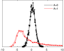
Consider, for example, the case in which we assume the data-generation process of Eq. (3), but the observed , , are generated from a modified version of Eq. (3) containing an extra non-linear term . The learned would not be able to describe this non-linear term, which would therefore be absorbed into the noise values , making the noise and dependent, as shown in Fig. 3(a).
To solve this issue, we propose to introduce an explicit latent variable for the generation of , i.e. , obtaining the GCM of Fig. 3(b). Define
where indicates the number of observations for which . We encourage to have small dependence on during training through the maximum mean discrepancy (MMD) criterion (Gretton et al., 2012). We can then use, e.g., the mean of , rather than , in Eq. (4). ( is Gaussian and can be computed analytically, see the Appendix).
Kusner et al. (2017), who also use a latent-variable approach, do not enforce small dependence. To demonstrate that this is necessary, we learned the parameters of the modified model with Gaussian distribution , using an expectation maximization approach. is shown in Fig. 3(a). As we can see, the extra term is absorbed by the latent variable. In other words, even if , the mismatch between the model and the observations implies .
In the next section, we explain how the approach described above can be implemented in a general algorithm that is applicable to complex, non-linear models.
4.1 Latent Inference-Projection Approach
For addressing a more general data-generation process mismatch than the one considered above, we need to explicitly incorporate a latent variable for each descendant of the sensitive attribute that needs to be corrected. General equations for the GCM of Fig. 2(c) with extra latent variables and are
If is categorical, , where can be any function, e.g. a neural network. If is continuous, is Gaussian with mean .
The model likelihood , and posterior distributions and required to form fair predictions, are generally intractable. We address this with a variational approach that computes Gaussian approximations and , of and respectively, parametrized by , as discussed in detail below.
After learning and , to form a fair prediction of a new instance , we proceed analogously to Eq. (4) using a Monte-Carlo approach: we first draw samples and , for , and then form
| (5) |
If we group the observed and latent variables as and respectively, the variational approximation to the intractable posterior is obtained by finding the variational parameters that minimize the Kullback-Leibler divergence . This is equivalent to maximizing a lower bound on the log marginal likelihood with
In our case, rather than , we use . Our approach is therefore to learn simultaneously the latent embedding and predictive distributions in Eq. (5). This could be preferable to other causal latent variable approaches such as the FairLearning algorithm proposed in Kusner et al. (2017), which separately learns a predictor of using samples from the previously inferred latent variables and from the non-descendants of .
In order for to be tractable conjugacy is required, which heavily restricts the family of models that can be used. This issue can be addressed with a Monte-Carlo approximation recently introduced in Kingma & Welling (2014) and Rezende et al. (2014). This approach represents as a non-linear transformation of a random variable from a parameter free distribution . As we choose to be Gaussian, with for the univariate case. This enables us to rewrite the bound as
The first part of the gradient of with respect to , , can be computed analytically, whilst the second part is approximated by
The variational parameters are parametrized by a neural network taking as input . In order to ensure that does not depend on , we follow a MMD penalization approach as in Louizos et al. (2016). This approach adds a MMD estimator term, approximated using random Fourier features, to the bound , weighted by a factor .
5 Experiments
In this section, we first show that our approach can disregard unfair information without a big loss in accuracy on a biased version of the Berkeley Admission dataset. We then test our method on two datasets previously considered in the causal and fairness literature, namely the UCI Adult and German Credit datasets. Experimental details are given in the Appendix.
5.1 The Berkeley Admission Dataset
In order to provide a test-case for our methodology, we consider the Berkeley Admission dataset, which contains sex , department choice , and admission decision for 4,526 applicants (all variables are categorical). Counts indicate that 45.5% of male applicants are admitted, versus only 30.4% of female applicants, i.e. . This discrepancy would appear to indicate gender bias. However, the potential outcome variable , resulting from intervening on , does not depend on . Therefore the dependence of on is entirely through department choice : the reason being that women are applying to departments with lower admission rates.
We modified the dataset to favor male applicants and to discriminate against female applicants, i.e. we added a direct path making dependent on . On this new dataset, when predicting using only the link through we obtained 67.9% accuracy, whilst when predicting using both and through () we obtained 71.6% accuracy, indicating that the link has a strong impact on the decision.
We used the latent inference-projection approach described in §4.1 to disregard the effect along the direct path . Whilst does not require correction, we nevertheless used a latent variable to test how much information about we lose by projecting into a latent space and back. As the bias along the path affects both male and female applicants, we could not use either of the two sexes as a baseline – instead, we averaged over values of sampled from .
We divided the dataset into training and test sets of sizes 3,500 and 1,026 respectively, and used for the Monte-Carlo approximation in Eq. (5). Our method gave a test accuracy of 67.1%, which is close to the desired 67.9%, indicating that we are disregarding the unfair information whilst only losing a small amount of information through latent inference-projection.
5.2 The UCI Adult Dataset
The Adult dataset from the UCI repository (Lichman, 2013) contains 14 attributes including age, working class, education level, marital status, occupation, relationship, race, gender, capital gain and loss, working hours, and nationality for 48,842 individuals; 32,561 and 16,281 for the training and test sets respectively. The goal is to predict whether the individual’s annual income is above or below $50,000. We assume the GCM of Fig. 4(a), where corresponds to the protected attribute sex, to the duple age and nationality, to marital status, to level of education, to the triple working class, occupation, and hours per week, and to the income class222We omit race, and capital gain and loss (although including capital gain and loss would increase test accuracy from 82.9% to 84.7%) to use the same attributes as in Nabi & Shpitser (2018).. Age, level of education and hours per week are continuous, whilst sex, nationality, marital status, working class, occupation, and income are categorical. Besides the direct effect , we would like to remove the effect of on through marital status, namely along the paths . This GCM is similar to the one analyzed in §3.2 and, except for the latent variables, is the same as the one used in Nabi & Shpitser (2018).
| 82.88% | 81.66% | 610.85 | 13.31 | 3.73 | 3.10 | 3.12 |
| 82.85% | 80.21% | 6.73 | 2.80 | 3.75 | 2.88 | 3.10 |
| 82.71% | 79.41% | 2.97 | 3.45 | 0.25 | 0.07 | 0.49 |
| 80.60% | 73.98% | 3.19 | 6.31 | 0.22 | 0.10 | 0.47 |
Nabi & Shpitser (2018) assume that all variables, except and are continuous, and linearly related, except for which where is the sigmoid function. With the encoding , where 0 indicates the male baseline value, and under the approximation , we can write the PSE in the odds ratio scale as . A new instance from the test set is classified by using . The test accuracy obtained by constraining the PSE to lie between 0.95 and 1.05 is 72%, compared to 82% of the unconstrained case.
In our method, for the MMD penalization we used a two stage approach, where a factor (no penalization) was used for the first 5,000 training steps, and a factor was used for the remaining training steps. For the Monte-Carlo approximation in Eq. (5), we used . These values were chosen based on accuracy/computational cost on the training set.
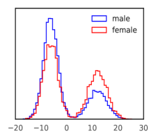
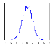
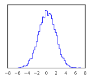
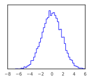
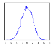
In Table 1, we show the unfair and fair accuracy on the test set at different stages of the training, together with the corresponding MMD values for and . As we can see, the MMD value for is drastically reduced from 5,000 to 8,000 and 15,000 training steps, without drastic loss in accuracy. After 20,000 training steps, the fair accuracy reduces to that of a dummy classifier. These results were obtained by performing counterfactual correction for both males and females, even if not required for males. Fair accuracy when performing counterfactual correction only for females is instead 82.80%, 80.05%, 80.87%, and 76.44% after 5,000, 8,000, 15,000 and 20,000 training steps respectively.
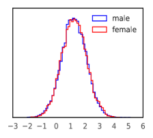
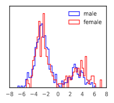
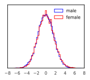
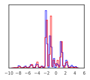
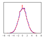
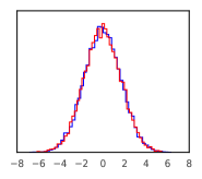
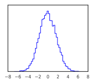
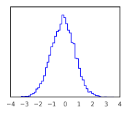
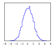
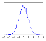
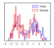
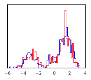
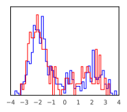
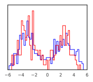
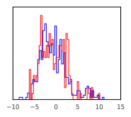
In Fig. 5, we show histograms of separately for males and females for increasing numbers of training steps. The remaining variables are shown in the Appendix. As can be seen, the addition of the MMD penalization to the variational bound for more training steps has the effect of reducing the number of modes in the posterior. From the evidence available, it is unclear if the shape changes are a necessary consequence of enforcing them to be similar, or if a simplification of the latent space is a more fundamental drawback of the MMD method. We leave any further investigations into such constraints for future work.


5.3 The UCI German Credit Dataset
The German Credit dataset from the UCI repository contains 20 attributes of 1,000 individuals applying for loans. Each applicant is classified as a good or bad credit risk, i.e. as likely or not likely to repay the loan. We assume the GCM in Fig. 4(b), where corresponds to the protected attribute sex, to age, to the triple status of checking account, savings, and housing, and the duple credit amount and repayment duration. The attributes age, credit amount, and repayment duration are continuous, whilst checking account, savings, and housing are categorical. Besides the direct effect , we would like to remove the effect of on through . We only need to introduce a hidden variable for , as does not need to be corrected.
We divided the dataset into training and test sets of sizes 700 and 300 respectively. We used for the first 2,000 training steps, and afterward. For the Monte-Carlo approximation in Eq. (5), we used . Counterfactual correction was performed for both males and females.
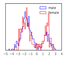
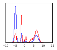
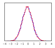
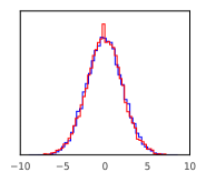
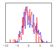
In Table 2, we show the unfair and fair test accuracy and the MMD values for after 2,000, 4,000, and 8,000 training steps (the results remain similar with a higher number of training steps). As we can see, unfair and fair accuracy, and MMD values are similar for all iterations. This indicates that, unlike the Adult dataset, model-observations mismatch is not problematic. This is confirmed by ; we learn a structured distribution which does not differ significantly for females and males. In Fig. 6, we show for one dimension of the variable housing, which shows the most significant difference between females and males. The remaining variables are shown in the Appendix.
6 Conclusions
| 74.67% | 73.67% | 1.12 | 2.82 | 5.47 |
| 76.33% | 76.00% | 1.23 | 2.38 | 2.27 |
| 76.00% | 76.00% | 1.27 | 2.20 | 1.79 |
We have introduced a latent inference-projection method to achieve path-specific counterfactual fairness which simplifies, generalizes and outperforms previous literature. A fair decision is achieved by correcting the variables that are descendants of the protected attribute along unfair pathways, rather than by imposing constraints on the model parameters. This enables us to retain fair information contained in the problematic descendants and to leave unaltered the underlying data-generation mechanism. In the future, we plan to investigate alternative techniques to MMD for enforcing independence between the latent space and the sensitive attribute.
References
- Berk et al. (2017) Berk, R., Heidari, H., Jabbari, S., Kearns, M., and Roth, A. Fairness in criminal justice risk assessments: The state state of the art. 2017.
- Bonchi et al. (2017) Bonchi, F., Hajian, S., Mishra, B., and Ramazzotti, D. Exposing the probabilistic causal structure of discrimination. International Journal of Data Science and Analytics, 3(1):1–21, 2017.
- Calmon et al. (2017) Calmon, F., Wei, D., Vinzamuri, B., Ramamurthy, K. N., and Varshney, K. R. Optimized pre-processing for discrimination prevention. In Advances in Neural Information Processing Systems 30, pp. 3995–4004, 2017.
- Chiappa (2014) Chiappa, S. Explicit-duration Markov switching models. Foundations and Trends in Machine Learning, 7(6):803–886, 2014.
- Chouldechova (2017) Chouldechova, A. Fair prediction with disparate impact: A study of bias in recidivism prediction instruments. Big Data, 5(2):153–163, 2017.
- Corbett-Davies et al. (2017) Corbett-Davies, S., Pierson, E., Feller, A., Goel, S., and Huq, A. Algorithmic decision making and the cost of fairness. In Proceedings of the 23rd ACM SIGKDD International Conference on Knowledge Discovery and Data Mining, pp. 797–806, 2017.
- Dawid (2007) Dawid, P. Fundamentals of statistical causality. Technical report, University Colledge London, 2007.
- Dieterich et al. (2016) Dieterich, W., Mendoza, C., and Brennan, T. Compas risk scales: Demonstrating accuracy equity and predictive parity, 2016.
- Dwork et al. (2012) Dwork, C., Hardt, M., Pitassi, T., Reingold, O., and Zemel, R. Fairness through awareness. In Proceedings of the 3rd Innovations in Theoretical Computer Science Conference, pp. 214–226, 2012.
- Edwards & Storkey (2016) Edwards, H. and Storkey, A. Censoring representations with an adversary. In 4th International Conference on Learning Representations, 2016.
- Feldman et al. (2015) Feldman, M., Friedler, S. A., Moeller, J., Scheidegger, C., and Venkatasubramanian, S. Certifying and removing disparate impact. In Proceedings of the 21th ACM SIGKDD International Conference on Knowledge Discovery and Data Mining, pp. 259–268, 2015.
- Gretton et al. (2012) Gretton, A., Borgwardt, K. M., Rasch, M. J., Schölkopf, B., and Smola, A. A kernel two-sample test. Journal of Machine Learning Research, 13:723–773, 2012.
- Hoffman et al. (2015) Hoffman, M., Kahn, L. B., and Li, D. Discretion in hiring, 2015.
- Kilbertus et al. (2017) Kilbertus, N., Rojas-Carulla, M., Parascandolo, G., Hardt, M., Janzing, D., and Schölkopf, B. Avoiding discrimination through causal reasoning. In Advances in Neural Information Processing Systems 30, pp. 656–666, 2017.
- Kingma & Ba (2015) Kingma, D. P. and Ba, J. Adam: A method for stochastic optimization. In 3rd International Conference on Learning Representations, 2015.
- Kingma & Welling (2014) Kingma, D. P. and Welling, M. Auto-encoding variational Bayes. In 2nd International Conference on Learning Representations, 2014.
- Kleinberg et al. (2016) Kleinberg, J., Mullainathan, S., and Raghavan, M. Inherent trade-offs in the fair determination of risk scores. In 8th Innovations in Theoretical Computer Science Conference, pp. 43:1–43:23, 2016.
- Kusner et al. (2017) Kusner, M. J., Loftus, J. R., Russell, C., and Silva, R. Counterfactual fairness. In Advances in Neural Information Processing Systems 30, pp. 4069–4079, 2017.
- Lichman (2013) Lichman, M. UCI machine learning repository, 2013. URL http://archive.ics.uci.edu/ml.
- Louizos et al. (2016) Louizos, C., Swersky, K., Li, Y., Welling, M., and Zemel, R. The variational fair autoencoder. In 4th International Conference on Learning Representations, 2016.
- Nabi & Shpitser (2018) Nabi, R. and Shpitser, I. Fair inference on outcomes. In Thirty-Second AAAI Conference on Artificial Intelligence, 2018.
- Pearl (2000) Pearl, J. Causality: Models, Reasoning, and Inference. Cambridge University Press, 2000.
- Pearl (2001) Pearl, J. Direct and indirect effects. In Proceedings of the Seventeenth Conference on Uncertainty in Artificial Intelligence, pp. 411–420, 2001.
- Pearl (2012) Pearl, J. The causal mediation formula – a guide to the assessment of pathways and mechanisms. Prevention Science, 13:426–436, 2012.
- Pearl et al. (2016) Pearl, J., Glymour, M., and Jewell, N. P. Causal Inference in Statistics: A Primer. Wiley, 2016.
- Peters et al. (2017) Peters, J., Janzing, D., and Schölkopf, B. Elements of Causal Inference: Foundations and Learning Algorithms. MIT Press, 2017.
- Qureshi et al. (2016) Qureshi, B., Kamiran, F., Karim, A., and Ruggieri, S. Causal discrimination discovery through propensity score analysis. ArXiv e-prints, 2016.
- Rezende et al. (2014) Rezende, D. J., Mohamed, S., and Wierstra, D. Stochastic backpropagation and approximate inference in deep generative models. In Proceedings of the 31st International Conference on Machine Learning, pp. 1278–1286, 2014.
- Russell et al. (2017) Russell, C., Kusner, M. J., Loftus, J., and Silva, R. When worlds collide: Integrating different counterfactual assumptions in fairness. In Advances in Neural Information Processing Systems 30, pp. 6417–6426, 2017.
- Shpitser (2013) Shpitser, I. Counterfactual graphical models for longitudinal mediation analysis with unobserved confounding. Cognitive Science, 37(6):1011–1035, 2013.
- Zafar et al. (2017) Zafar, B., Valera, I., Gomez-Rodriguez, M., and Gummadi, K. Fairness constraints: Mechanisms for fair classification. In 20th International Conference on Artificial Intelligence and Statistics, 2017.
- Zemel et al. (2013) Zemel, R, Wu, Y., Swersky, K., Pitassi, T., and Dwork, C. Learning fair representations. In Proceedings of the 30th International Conference on Machine Learning, pp. 325–333, 2013.
- Zeng et al. (2016) Zeng, J., Ustun, B., and Rudin, C. Interpretable classification models for recidivism prediction. Journal of the Royal Stat. Soc.: Series A (Statistics in Society), 2016.
- Zhang et al. (2018) Zhang, B., Lemoine, H, and Mitchell, M. Mitigating unwanted biases with adversarial learning. In Proceedings of the 1st AAAI/ACM Conference on AI, Ethics, and Society, 2018.
- Zhang & Bareinboim (2018) Zhang, J. and Bareinboim, E. Fairness in decision-making – the causal explanation formula. In Proceedings of the 32nd AAAI Conference on Artificial Intelligence, 2018.
- Zhang & Wu (2017) Zhang, L. and Wu, X. Anti-discrimination learning: a causal modeling-based framework. International Journal of Data Science and Analytics, pp. 1–16, 2017.
- Zhang et al. (2017) Zhang, L., Wu, Y., and Wu, X. A causal framework for discovering and removing direct and indirect discrimination. In IJCAI, pp. 3929–3935, 2017.
Appendix A Identifiability of PSE
We summarize the method described in Shpitser (2013) to graphically establish whether a PSE is identifiable.
Acyclic Directed Mixed Graph (ADMG):
An ADMG is a causal graph containing two kinds of links, directed links (either green or black depending on whether we are interested in the corresponding causal path), and red bidirected links, indicating the presence of an unobserved common cause. The ADMG corresponding to Fig. 7(a) is given by Fig. 7(b).
District:
The set of nodes in an ADMG that are reachable from through bidirected paths is called the district of . For example, the district of in Fig. 7(b) is .
Recanting District:
Let be an ADMG, and a subset of causal paths which start in and end in . Let be the set of potential causes of that differ from and that influence through causal paths that do not intersect . Let be the subgraph of containing only the nodes in . A district in is called the recanting district for the effect of on along the paths in if there exist nodes such that there is a causal path and a causal path . If contains a recanting district for , then the effect along is non-identifiable.
For example, the set in Fig. 7(b) is . The districts in are . This district is recanting for the effect along , as , whilst . (This district is not recanting for the effect along .)
Appendix B Latent-Variable Conditional Distribution
Consider the GCM in Fig. 3(a), corresponding to Eq. (3) with the addition of a Gaussian latent variable in the equation for . The joint distribution is Gaussian with exponent proportional to with
The Gaussian conditional can be computed through the formulas for Gaussian marginalization and conditioning.


Appendix C Experimental Details
For all datasets, as the prior distribution for each latent variable we used a mixture of two-dimensional Gaussians with ten mixture components and diagonal covariances. As the variational posterior distribution we used a two-dimensional Gaussian with diagonal covariance, with means and log variances obtained as the outputs of a neural network with two linear layers of size 20 and tanh activation, followed by a linear layer. In the conditional distributions, was a neural network with one linear layer of size 100 with tanh activation, followed by a linear layer. The outputs were Gaussian means for continuous variables and logits for categorical variables. We used the Adam optimizer (Kingma & Ba, 2015) with learning rate 0.01, mini-batch size 128, and default values , , and -8.
C.1 UCI Adult Dataset
In Fig. 8 we show histograms for prior and posterior distributions in the latent space.
C.2 UCI German Credit Dataset


In Fig. 9 we show histograms for posterior distributions in the latent space.