Optimal inventory management and order book modeling

Abstract

We model the behavior of three agent classes acting dynamically in a limit order book of a financial asset. Namely, we consider market makers (MM), high-frequency trading (HFT) firms, and institutional brokers (IB). Given a prior dynamic of the order book, similar to the one considered in the Queue-Reactive models [12, 18, 19], the MM and the HFT define their trading strategy by optimizing the expected utility of terminal wealth, while the IB has a prescheduled task to sell or buy many shares of the considered asset. We derive the variational partial differential equations that characterize the value functions of the MM and HFT and explain how almost optimal control can be deduced from them. We then provide a first illustration of the interactions that can take place between these different market participants by simulating the dynamic of an order book in which each of them plays his own (optimal) strategy.

Key words: Optimal trading, market impact, optimal control.
MSC 2010: 49L20, 49L25.

1 Introduction

The comprehension of the order book dynamic has become a fundamental issue for all market participants and for regulators that try to increase the market transparency and efficiency. A deep understanding of the order book dynamic and agents behaviors enables: market makers to ensure liquidity provision at cheaper prices, high-frequency traders to reduce arbitrage opportunities, investors to reduce their transaction costs, policy makers to design relevant rules, to strengthen market transparency and to reduce market manipulation. Moreover, modeling the order book provides insights on the behavior of the price at larger time scales since the price formation process starts at the order book level, see e.g. [11] for Brownian diffusion asymptotic of rescaled price processes. Recently, the widespread market electronification has facilitated the access of high quality data describing market participants decisions and interactions at the finest time scale, on which statistics can be based. The availability of the order book data certainly allows a better understanding of the market activity. On the other hand, the recent market fragmentation and the increase of trading frequency rise the complexity of agents actions and interactions.

The main objective of the present paper is to propose a flexible order book dynamics model close to the one of [12, 18, 19, 23], construct a first building block towards a realistic order book modeling, and try to better understand the various regimes related to the presence of different market participants. Instead of considering a pure statistical dynamics as in e.g. [12], we construct a structural endogenous dynamics, see e.g. [22, 23], based on the optimal behavior of agents that are assumed to be rational. For numerical tractability, we simplify the market in three classes of (most significant) participants: the market makers (MM), the high-frequency trading (HFT) firms, and the institutional brokers (IB). Each of them decides of his policy in an optimal way, given prior statistics, and then interact with the others given the endogenous realizations of the market.

More precisely, we postulate that they assume an order book model similar to the one suggested by the Queue-Reactive model [18], see also [1, 12, 17], in which we restrict to the best bid and ask queues: limit and aggressive orders arrive with certain intensities, when a queue is depleted it is regenerated according to a certain law and possibly after a price move, the spread can take two different values. Importantly, we also take the order book’s imbalance into account in the modeling of the different transition probabilities, see e.g. Besson et al. [9].

The market participants can either put limit or aggressive orders. The aim of a market maker is to gain the spread. He should therefore essentially put limit orders, aggressive orders being used when his inventory is too unbalanced. In our model, he can only acts on the given order book. The high-frequency trader is assumed to play on the correlation between the order book dynamics, viewed as the stock price, and the price of another asset, called futures hereafter. Indeed, he believes that the difference between the stock and the futures prices is mean-reverting. Whenever he buys/sells one unit of the stock, he sells/buys back one unit of the futures. We do not handle the order book associated to the futures but simply model the price of the futures as the mid-price of the stock to which a mean-reverting process is added. Still, we introduce a (possibly equal to $0$) transaction cost proportional to the size of the transaction. As the market-makers, he seeks for a zero inventory at the end of the trading period. Finally, institutional brokers are simply assumed to play VWAP (Volume Weighted Average Price)- or Volume-based strategies (trading algorithms). Again, they essentially use limit orders and become aggressive when they are too late in their schedule.

We focus on the derivation of the optimal strategies of the market makers and the high-frequency traders, and on how they can be computed numerically by solving the associated variational partial differential equations. Note that it is important to consider their strategies within a dynamical model as current actions impact the order book and therefore may modify its futures dynamics. We will actually see that, in certain situations, participants can place aggressive orders or limit orders in the spread just to try to manipulate the order book’s dynamics in a favorable way. Note that the dimension of our control space is higher than in [1, 17, 22, 23] since more complex decisions are required to tackle the market making problem.

However, the ultimate goal of this work is to provide a market simulator. In the last section, we already present simulations of the market behavior given the pre-computed optimal strategies of the different actors. More precisely, we will only simulate the evolution of the mean-reverting process (driving the difference between the stock and the futures price) together with the reconstruction of the queues when prices move, and let the participants play their optimal strategies given the evolution of the order book due to their different actions. This should allow us to study how these different market participants may interact among each other if each of them is playing his optimal policy. In particular, one should observe different market regimes depending on the proportion of the different participants in the total population, on their risk aversion, etc. First simulations are provided in this paper, a more throughout study is left for future research.

Our approach therefore lies in between two current streams of literature. The first one is based on “general equilibrium models”, including economic models, where the market activity is generated by interactions between rational agents who take optimal decisions that interact through the market netting process, see e.g. [14, 24, 25]. The second stream of literature considers purely statistical models where the order book is seen as a random process, see e.g. [2, 3, 8, 12, 13, 16, 18, 19, 20, 21, 26]. The statistical models focus on reproducing many salient features of a real market rather than agents behaviors and interactions. In our approach, we take into account that the agent’s behavior are essentially based on statistical approaches, but that they eventually interact with each other.

We end this introduction with an outline of our paper. In Section 2, we present the general order book dynamics. The marker maker control problem is studied in details in Section 3. There, we present the equations satisfied by their optimal strategy and propose a numerical solution for this problem, together with numerical illustrations. In Section 4, we formulate the high-frequency trader control problem and perform a similar analysis. The institutional broker strategy is described in Section 5, where we restrict to VWAP and Volume liquidation problems. Finally, in Section 6, we simulate a realistic market using the three agent’s optimal trading strategies.

2 General order book presentation and priors of the market participants

As mentioned above, we focus on a single order book and only model the best bid and ask prices, in a similar way to [12]. In this section, we describe the general market mechanisms as well as the priors on which the optimal strategies of the agents are based. We fix a terminal time horizon $T$ and consider a probability space $(\Omega,\mathbb{P})$. Here, $\Omega:=\Omega_{1}\times\Omega_{2}$ and $\mathbb{P}:=\mathbb{P}_{1}\otimes\mathbb{P}_{2}$, where $\Omega_{1}$ is the space of $\mathbb{R}^{11}$-valued cadlag paths on $[0,T]$ endowed with a probability measure $\mathbb{P}_{1}$ with full support on $\Omega_{1}$, and $\Omega_{2}$ is the one dimensional Wiener space endowed with the Wiener measure $\mathbb{P}_{2}$.

We denote respectively by $(P^{\mathfrak{b}}_{t})_{t\geq 0}$ and $(P^{\mathfrak{a}}_{t})_{t\geq 0}$ the best bid offer and the best ask offer processes on the market. They are valued in ${\mathfrak{d}}\mathbb{Z}$ where ${\mathfrak{d}}>0$ is the tick size. We denote by $(Q^{\mathfrak{b}}_{t})_{t\geq 0}$ and $(Q^{\mathfrak{a}}_{t})_{t\geq 0}$ the sizes of the corresponding queues valued in $\mathbb{N}^{*}$. To simplify the notation, we introduce $P:=(P^{\mathfrak{b}},P^{\mathfrak{a}})$, $Q:=(Q^{\mathfrak{b}},Q^{\mathfrak{a}})$ and define the spread process as $\delta P:=P^{\mathfrak{a}}-P^{\mathfrak{b}}$. Moreover, we assume that $\delta P_{t}\in\{{\mathfrak{d}},2{\mathfrak{d}}\}$ for all $t\geq 0$.

We denote by $(\tau_{i})_{i\geq 1}$ the times at which orders are sent to the market. We assume that this sequence is increasing and that $\#\{i\in\mathbb{N}:\tau_{i}<T\}<\infty$ a.s. The market participants can send different types of orders at each time $\tau_{i}$:

• Aggressive orders of size $\alpha^{\mathfrak{b}}_{i}\in\mathbb{N}\cap[0,Q^{\mathfrak{b}}]$ at the bid or of size $\alpha^{\mathfrak{a}}_{i}\in\mathbb{N}\cap[0,Q^{\mathfrak{a}}]$ at the ask: the size of the corresponding queue, $Q^{\mathfrak{b}}$ or $Q^{\mathfrak{a}}$, decreases by the size of the aggressive order, $\alpha^{\mathfrak{b}}_{i}$ or $\alpha^{\mathfrak{a}}_{i}$.

• Limit orders of size $L^{\mathfrak{b}}_{i}\in\mathbb{N}$ at the bid or of size $L^{\mathfrak{a}}_{i}\in\mathbb{N}$ at the ask: the size of the corresponding queue, $Q^{\mathfrak{b}}$ or $Q^{\mathfrak{a}}$, increases by the size of the limit order, $L^{\mathfrak{b}}_{i}$ or $L^{\mathfrak{a}}_{i}$.

• When $\delta P=2{\mathfrak{d}}$: Limit orders of size $L^{\mathfrak{b},\frac{1}{2}}_{i}\in\mathbb{N}$ at the bid or of size $L^{\mathfrak{a},\frac{1}{2}}_{i}\in\mathbb{N}$ at the ask: the order is placed inside the spread, at the price $P^{\mathfrak{b}}+{\mathfrak{d}}=P^{\mathfrak{a}}-{\mathfrak{d}}$, this generates a new queue at the bid or at the ask, of size $L^{\mathfrak{b},\frac{1}{2}}_{i}$ or $L^{\mathfrak{a},\frac{1}{2}}_{i}$, and a price move.

• Cancellations: Cancellations of $M^{\mathfrak{b}}_{i}\in\mathbb{N}\cap[0,Q^{\mathfrak{b}}]$ orders at the bid or of $M^{\mathfrak{a}}_{i}\in\mathbb{N}\cap[0,Q^{\mathfrak{a}}]$ orders at the ask. The difference between cancellations and aggressive orders is that aggressive orders consume the bottom of the limit while we see cancellations as only consuming the top of the limit first.

We assume that the sequence $(\alpha^{\mathfrak{b}}_{i},\alpha^{\mathfrak{a}}_{i},L^{\mathfrak{b}}_{i},L^{\mathfrak{a}}_{i},L^{\mathfrak{b},\frac{1}{2}}_{i},L^{\mathfrak{a},\frac{1}{2}}_{i},M^{\mathfrak{b}}_{i},M^{\mathfrak{a}}_{i})_{i\geq 1}$ is made of random variables leaving, with probability one, on the state space $\mathbf{C}_{\circ}$ defined as the collection of elements $(a^{\mathfrak{b}},a^{\mathfrak{a}},\ell^{\mathfrak{b}},\ell^{\mathfrak{a}},\ell^{\mathfrak{b},\frac{1}{2}},$ $\ell^{\mathfrak{a},\frac{1}{2}},m^{\mathfrak{b}},$ $m^{\mathfrak{a}})$ $\in\mathbb{N}^{8}$ such that

$$\left\{\begin{array}[]{l}a^{\mathfrak{b}}a^{\mathfrak{a}}=0\\ \ell^{\mathfrak{b}}=\ell^{\mathfrak{a}}=0\;\mbox{ if }\max\{a^{\mathfrak{b}},a^{\mathfrak{a}}\}\geq 1\\ \ell^{\mathfrak{b},\frac{1}{2}}=0\;\mbox{ if }\max\{a^{\mathfrak{b}},a^{\mathfrak{a}},\ell^{\mathfrak{b}}\}\geq 1\\ \ell^{\mathfrak{a},\frac{1}{2}}=0\;\mbox{if }\max\{a^{\mathfrak{b}},a^{\mathfrak{a}},\ell^{\mathfrak{a}}\}\geq 1\\ m^{\mathfrak{b}}=0\;\mbox{ if }\max\{a^{\mathfrak{b}},a^{\mathfrak{a}},\ell^{\mathfrak{b}},\ell^{\mathfrak{b},\frac{1}{2}}\}\geq 1\\ m^{\mathfrak{a}}=0\;\mbox{if }\max\{a^{\mathfrak{b}},a^{\mathfrak{a}},\ell^{\mathfrak{a}},\ell^{\mathfrak{a},\frac{1}{2}}\}\geq 1\end{array}\right..$$ (2.7)

We interpret the above expression as follows. First, aggressive orders can not be sent simultaneously at the bid and at the ask. Next, limit orders (at the current bid/ask prices) can not be placed at the same time that aggressive orders are sent. Finally, one can not place limit orders within the spread if limit orders at the current bid/ask prices are placed. Because we only consider the first limits, these conditions are natural whenever one presumes that orders of different market participants do not arrive exactly at the same time.

Depending on the arrival of orders, queues can be depleted. In this case, new queues can be re-generated, at the same prices or at different prices, and possibly with a change of the spread value. To model this, we introduces a sequence of random variables $(\epsilon_{i},\epsilon^{\mathfrak{b}}_{i},\epsilon^{\mathfrak{a}}_{i})_{i\geq 1}$ with values in $\{0,1\}\times(\mathbb{N}^{*})^{2}$. The sequence $(\epsilon_{i})_{i\geq 1}$ will describe possible jumps of the bid/ask prices, while the sequence $(\epsilon^{\mathfrak{b}}_{i},\epsilon^{\mathfrak{a}}_{i})_{i\geq 1}$ will describe the new sizes of the queues when they are re-generated, after one of them is depleted. More precisely, we postulate the dynamics

$$\begin{array}[]{rl}P^{\mathfrak{b}}_{\tau_{i}}=&P^{\mathfrak{b}}_{\tau_{i-1}}+{\mathfrak{d}}\left[\mathbf{1}_{\{\epsilon_{i}=1\}}\left(-\mathbf{1}_{\{Q^{\mathfrak{b}}_{\tau_{i-1}}=\hat{\alpha}^{\mathfrak{b}}_{i}\}}+\mathbf{1}_{\{\delta P_{\tau_{i-1}}=2{\mathfrak{d}}\}}\mathbf{1}_{\{Q^{\mathfrak{a}}_{\tau_{i-1}}=\hat{\alpha}^{\mathfrak{a}}_{i}\}}\right)+\mathbf{1}_{\{L^{\mathfrak{b},\frac{1}{2}}_{i}>0\}}\right]\\ P^{\mathfrak{a}}_{\tau_{i}}=&P^{\mathfrak{a}}_{\tau_{i-1}}+{\mathfrak{d}}\left[\mathbf{1}_{\{\epsilon_{i}=1\}}\left(\mathbf{1}_{\{Q^{\mathfrak{a}}_{\tau_{i-1}}=\hat{\alpha}^{\mathfrak{a}}_{i}\}}-\mathbf{1}_{\{\delta P_{\tau_{i-1}}=2{\mathfrak{d}}\}}\mathbf{1}_{\{Q^{\mathfrak{b}}_{\tau_{i-1}}=\hat{\alpha}^{\mathfrak{b}}_{i}\}}\right)-\mathbf{1}_{\{L^{\mathfrak{a},\frac{1}{2}}_{i}>0\}}\right]\\ Q^{\mathfrak{b}}_{\tau_{i}}=&Q^{\mathfrak{b}}_{\tau_{i-1}}+L^{\mathfrak{b}}_{i}+(L^{\mathfrak{b},\frac{1}{2}}_{i}-Q^{\mathfrak{b}}_{\tau_{i-1}})\mathbf{1}_{\{L^{\mathfrak{b},\frac{1}{2}}_{i}>0\}}-\hat{\alpha}^{\mathfrak{b}}_{i}\mathbf{1}_{\{\Delta P^{\mathfrak{b}}_{\tau_{i}}=0\}}+(\epsilon^{\mathfrak{b}}_{i}-Q^{\mathfrak{b}}_{\tau_{i-1}})\mathbf{1}_{\{\Delta P^{\mathfrak{b}}_{\tau_{i}}\neq 0\}\cup\{{\hat{\alpha}^{\mathfrak{b}}_{i}=Q^{\mathfrak{b}}_{\tau_{i-1}}}\}}\\ Q^{\mathfrak{a}}_{\tau_{i}}=&Q^{\mathfrak{a}}_{\tau_{i-1}}+L^{\mathfrak{a}}_{i}+(L^{\mathfrak{a},\frac{1}{2}}_{i}-Q^{\mathfrak{a}}_{\tau_{i-1}})\mathbf{1}_{\{L^{\mathfrak{a},\frac{1}{2}}_{i}>0\}}-\hat{\alpha}^{\mathfrak{a}}_{i}\mathbf{1}_{\{\Delta P^{\mathfrak{a}}_{\tau_{i}}=0\}}+(\epsilon^{\mathfrak{a}}_{i}-Q^{\mathfrak{a}}_{\tau_{i-1}})\mathbf{1}_{\{\Delta P^{\mathfrak{a}}_{\tau_{i}}\neq 0\}\cup\{{\hat{\alpha}^{\mathfrak{a}}_{i}=Q^{\mathfrak{a}}_{\tau_{i-1}}}\}}\end{array}$$ (2.12)

for $i\geq 1$, where

$$\hat{\alpha}^{\mathfrak{b}/\mathfrak{a}}_{i}:=\alpha^{\mathfrak{b}/\mathfrak{a}}_{i}+M^{\mathfrak{b}/\mathfrak{a}}_{i},$$

with

$$(P^{\mathfrak{b}}_{0},P^{\mathfrak{a}}_{0},Q^{\mathfrak{b}}_{0},Q^{\mathfrak{a}}_{0})\in D_{P,Q}:=\{(p^{\mathfrak{b}},p^{\mathfrak{a}},q)\in({\mathfrak{d}}\mathbb{Z})^{2}\times(\mathbb{N}^{*})^{2}:p^{\mathfrak{a}}-p^{\mathfrak{b}}\in\{{\mathfrak{d}},2{\mathfrak{d}}\}\},$$

and the convention $\tau_{0}=0-$. We refer to (2.7) to see that this dynamics is consistent. In particular, prices can move only if one of the queues is depleted because of the arrival of aggressive orders or if a new limit order is inserted within the spread. These two situations can not occur simultaneously. The ask price can move by ${\mathfrak{d}}$ when the ask queue is depleted. If the spread was already $2{\mathfrak{d}}$, then the bid price moves up as well. The other way around if the bid queue is depleted. In the following, we extend the dynamics of $(P,Q)$ by considering it as a step constant right-continuous process on $[0,T]$.

We now denote by ${\cal E}$ the $\mathbb{N}^{{12}}$-valued step constant right-continuous process defined by

$$\Delta{\cal E}_{\tau_{i}}:={\cal E}_{\tau_{i}}-{\cal E}_{\tau_{i-1}}:=(\alpha^{\mathfrak{b}}_{i},\alpha^{\mathfrak{a}}_{i},L^{\mathfrak{b}}_{i},L^{\mathfrak{a}}_{i},L^{\mathfrak{b},\frac{1}{2}}_{i},L^{\mathfrak{a},\frac{1}{2}}_{i},{M^{\mathfrak{b}}_{i},M^{\mathfrak{a}}_{i},}\epsilon_{i},\epsilon^{\mathfrak{b}}_{i},\epsilon^{\mathfrak{a}}_{i},1),\;i\geq 1,$$

with ${\cal E}_{\tau_{0}}:={\cal E}_{0}:=0$. Later on, we shall only write

$$(P_{\tau_{i}},Q_{\tau_{i}})={\cal T}_{P,Q}(P_{\tau_{i-1}},Q_{\tau_{i-1}},\Delta{\cal E}_{\tau_{i}})$$ (2.13)

in which the map ${\cal T}_{P,Q}$ is defined explicitly by (2.12).

The process ${\cal E}$ models the flow of all the orders on the market. From the viewpoint of a market participant, it corresponds to its own orders and to the other participants’ orders that we denote by $\tilde{\cal E}$. The process $\tilde{\cal E}$ has jump times $(\tilde{\tau}_{i})_{i\geq 1}\subset(\tau_{i})_{i\geq 1}$ of sizes

$$\Delta\tilde{\cal E}_{\tilde{\tau}_{i}}=\sum_{j\geq 1}{\bf 1}_{\{\tilde{\tau}_{i}=\tau_{j}\}}\Delta{\cal E}_{\tau_{j}},\;i\geq 1.$$ (2.14)

It induces a counting measure $\tilde{\nu}(dt,de)$. For a market participant, a prior on this measure is given by the compensator $\tilde{\mu}$ of $\tilde{\nu}$ under $\mathbb{P}$. We assume that it is state dependent. More precisely, we consider a Borel kernel $(p,q)\in D_{P,Q}\mapsto\tilde{\mu}(\cdot|p,q)\in{\cal M}([0,T]\times\mathbb{N}^{{8}})$, where ${\cal M}([0,T]\times\mathbb{N}^{{8}})$ denotes the collection of non-negative measures on $[0,T]\times\mathbb{N}^{{8}}$. In particular, it can depend on the order book’s imbalance, as observed in e.g. [9]. To be consistent with the constraints imposed above, it satisfies:

$$\tilde{\mu}(\cdot|p,q)\mbox{ is supported by }\mathbf{C}_{\circ},\;\mbox{ for all }(p,q)\in D_{P,Q}.$$ (2.15)

It should also be such that aggressive orders and cancellations are never bigger than the corresponding queue size, which will be made more explicit in our numerical example sections, see Section 3.4.

Next, we shall denote by ${\cal E}^{\phi}$ the flows corresponding to the trading strategy of either a market maker, a high-frequency trader, or an institutional broker. Thus, she will assume facing a global flow ${\cal E}=\tilde{\cal E}+{\cal E}^{\phi}$.

Moreover, for simplicity, we shall assume that $\tilde{\mu}$ is of the form

$$d\tilde{\mu}(c,\varepsilon,\varepsilon^{\mathfrak{b}},\varepsilon^{\mathfrak{a}},dt|p,q)=d\lambda(\varepsilon,\varepsilon^{\mathfrak{b}},\varepsilon^{\mathfrak{a}}|p,q,c)d\beta(c|p,q)dt$$ (2.16)

in which $\lambda$ and $\beta$ are bounded Borel non-negative kernels and (without loss of generality)

$$\int d\lambda(\varepsilon,\varepsilon^{\mathfrak{b}},\varepsilon^{\mathfrak{a}}|p,q,c)=1,\;\mbox{ for all }(p,q,c)\in D_{P,Q}\times\mathbf{C}_{\circ}.$$ (2.17)

Later on, when an order $(\alpha^{\mathfrak{b}}_{i},\alpha^{\mathfrak{a}}_{i},L^{\mathfrak{b}}_{i},L^{\mathfrak{a}}_{i},L^{\mathfrak{b},\frac{1}{2}}_{i},L^{\mathfrak{a},\frac{1}{2}}_{i},{M^{\mathfrak{b}}_{i},M^{\mathfrak{a}}_{i})}$ is sent by a MM, an HFT or an IB, we shall also assume that the conditional law of $(\epsilon_{i},\epsilon^{\mathfrak{b}}_{i},\epsilon^{\mathfrak{a}}_{i})$ is given by $\lambda$.

Remark 2.1.

Let $\gamma(p,q):=\int d\beta(c|p,q)$. Then, $\gamma$ is uniformly bounded by the above assumption. Let $\tau$ be a stopping time and fix $h>0$. Since $\lambda$ integrates to one, it follows that $\mathbb{P}[\#\{t\in[\tau,\tau+h]:\Delta\tilde{\cal E}_{t}\neq 0\}=1|{\cal F}_{\tau}]=h\gamma(P_{\tau},Q_{\tau})+o(h)$ and $\mathbb{P}[\#\{t\in[\tau,\tau+h]:\Delta\tilde{\cal E}_{t}\neq 0\}>1|{\cal F}_{\tau}]=o(h)$. Moreover, the process counting the number of jumps of $\tilde{\cal E}$ is dominated by a Poisson process with intensity $\bar{\gamma}:=\sup\gamma<\infty$. Hence, $\mathbb{P}[\#\{t\leq T:\Delta\tilde{\cal E}_{t}\neq 0\}\geq k]\leq\bar{\gamma}T/k$, for $k\geq 1$, by Markov’s inequality. Similarly, if $g$ is a non-decreasing Borel map, then $\mathbb{E}[g(\#\{t\in[0,T]:\Delta\tilde{\cal E}_{t}\neq 0\})]\leq\sum_{k\geq 1}g(k)\frac{(\bar{\gamma}T)^{k}}{k!}e^{-\bar{\gamma}T}$.

3 Market maker’s optimal control problem

In this section, we describe the optimal control problem of the market maker, the key tools to characterize the solution and how to numerically approximate the optimal control.

3.1 Market maker’s strategy and state dynamics

The market maker typically places limit orders in order to make profit of the spread but can turn aggressive when his inventory is too important. At the end the trading period $[0,T]$, the later should be zero. In the following, we denote by $G$ his gain process and by $I$ his inventory. We also need to keep track of the sizes of his orders already placed at the bid queue, $N^{\mathfrak{b}}$, and at the ask queue, $N^{\mathfrak{a}}$. For simplicity, we impose that new orders can not be placed at the bid (respectively at the ask) if he already has previously taken a position at the bid (respectively at the ask). Then, his position at the bid (resp. at the ask) is completely described by $N^{\mathfrak{b}}$ (resp. $N^{\mathfrak{a}}$) and the number of units $B^{\mathfrak{b}}$ before him in the bid-queue (resp. $B^{\mathfrak{a}}$ before him in the ask-queue). Later on, we only write $N=(N^{\mathfrak{b}},N^{\mathfrak{a}})$ and $B=(B^{\mathfrak{b}},B^{\mathfrak{a}})$.

To define the market maker’s control, we assume that he faces the exogenous process $\tilde{\cal E}$ described in Section 2.

For him, a control is a sequence of random variables $\phi=(\tau^{\phi}_{i},\mathbf{c}^{\phi}_{i})_{i\geq 1}$ where $(\tau^{\phi}_{i})_{i\geq 1}$ is an increasing sequence of times and each $\mathbf{c}^{\phi}_{i}=(\alpha_{i}^{\mathfrak{b},\phi},\alpha_{i}^{\mathfrak{a},\phi},L_{i}^{\mathfrak{b},\phi},L_{i}^{\mathfrak{a},\phi},L_{i}^{\mathfrak{b},\frac{1}{2},\phi},L_{i}^{\mathfrak{a},\frac{1}{2},\phi},M_{i}^{\mathfrak{b},\phi},M_{i}^{\mathfrak{a},{\phi}})$ is $\mathbf{C}_{\circ}$-valued, see below for more implicit restrictions. The times $(\tau_{i}^{\phi})_{i\geq 1}$ are the times at which he sends orders: the action done at $\tau^{\phi}_{i}$ is $\mathbf{c}^{\phi}_{i}$, whose components have the same meanings as in Section 2.

Given his own orders and the other participants’ orders, the sequence of times at which orders are sent to the market is $(\tau_{i})_{i\geq 1}$ where $\tau_{0}:={0-}$ and $\tau_{i+1}=\min\{\tilde{\tau}_{j}>\tau_{i},\;j\geq 1\}\wedge\min\{\tau^{\phi}_{j}>\tau_{i},\;j\geq 1\}$, see (2.14) and above.

We denote by ${\cal E}^{\phi}$ the càdlàg process that jumps only at the times $\tau_{i}^{\phi}$s with jump size

$$\Delta{\cal E}^{\phi}_{\tau^{\phi}_{i}}=(\mathbf{c}^{\phi}_{i},\sum_{j\geq 1}(\epsilon_{j},\epsilon^{\mathfrak{b}}_{j},\epsilon^{\mathfrak{a}}_{j}){\bf 1}_{\{\tau^{\phi}_{i}=\tau_{j}\}}),\;i\geq 1,$$

so that

$${\cal E}={\cal E}^{\phi}+\tilde{\cal E}$$

from his point of view. As usual, we impose that ${\cal E}^{\phi}$ is predictable for the (completed) filtration $\mathbb{F}^{\phi}=({\cal F}^{\phi}_{t})_{t\geq 0}$ generated by ${\cal E}$. We will also keep in mind the number of actions

$$J:=\sum_{i\geq 1}{\bf 1}_{\{\tau^{\phi}_{i}\leq\cdot\}}$$

from time $0$ on, as it may induce a cost.

We now impose a minimum and maximum inventory size, denoted by $(-I^{*},I^{*})\in(-\mathbb{N})\times\mathbb{N}$, and that

$$\#\{\tau^{\phi}_{i}\leq T,i\geq 1\}\leq k_{\phi}\wedge J_{\circ}~{}a.s.,\mbox{ for some }k_{\phi}\in\mathbb{N},$$

for some $J_{\circ}\in\mathbb{N}\cup\{\infty\}$. The constraint on the inventory is classic. The constraint on the number of operations can be justified by operational constraints. In the case $J_{\circ}=\infty$, it just means that each control should be of essentially bounded activity, but the bound is not uniform on the set of controls and can be as large as needed.

To be admissible, a control $\phi$ should therefore be such that each $\mathbf{c}^{\phi}_{i}$ is $\mathbf{C}(Z_{\tau^{\phi}_{i}-})$-valued, where

$$Z:=(P,Q,X)\;\mbox{ with }\;X:=(G,I,N,B,J),$$

and, for $z=(p^{\mathfrak{b}},p^{\mathfrak{a}},q^{\mathfrak{b}},q^{\mathfrak{a}},g,i,n^{\mathfrak{b}},n^{\mathfrak{a}},b^{\mathfrak{b}},b^{\mathfrak{a}},j)$, $\mathbf{C}(z)$ is the collection of elements $c:=(a^{\mathfrak{b}},a^{\mathfrak{a}},\ell^{\mathfrak{b}},$ $\ell^{\mathfrak{a}},\ell^{\mathfrak{b},\frac{1}{2}},$ $\ell^{\mathfrak{a},\frac{1}{2}},$ $m^{\mathfrak{b}},$ $m^{\mathfrak{a}})\in\mathbf{C}_{\circ}\setminus\{0\}$ such that :

$$a^{\mathfrak{b}}\leq\min\left\{i+I^{*}-b^{\mathfrak{a}}\;;\;q^{\mathfrak{b}}\right\}\;, \;a^{\mathfrak{a}}\leq\min\left\{I^{*}-i-b^{\mathfrak{b}}\;;\;q^{\mathfrak{a}}\right\},$$

$$\ell^{\mathfrak{b}}\leq(I^{*}-i){\bf 1}_{\{{n^{\mathfrak{b}}=0}\}}\;, \;\ell^{\mathfrak{a}}\leq(i+I^{*}){\bf 1}_{\{n^{\mathfrak{a}}=0\}},$$

$$\ell^{\mathfrak{b},\frac{1}{2}}\leq(I^{*}-i){\bf 1}_{\{p^{\mathfrak{a}}-p^{\mathfrak{b}}=2{\mathfrak{d}}\}}{\bf 1}_{\{{n^{\mathfrak{b}}=0}\}}\;, \;\ell^{\mathfrak{a},\frac{1}{2}}\leq(i+I^{*}){\bf 1}_{\{p^{\mathfrak{a}}-p^{\mathfrak{b}}=2{\mathfrak{d}}\}}{\bf 1}_{\{{n^{\mathfrak{a}}=0}\}}$$

$$m^{\mathfrak{b}}\leq n^{\mathfrak{b}}\; ,\;m^{\mathfrak{a}}\leq n^{\mathfrak{a}}$$

$$c=0 \mbox{ if }j=J_{\circ}.$$

Note that the constraints on the first three lines correspond to the fact that we do not want to take a position that could lead to an inventory out of the limits $-I^{*}$ and $I^{*}$ if it was suddenly executed. The indicator functions correspond to additional constraints on the controls, imposed for numerical tractability: no new limit order can be sent on a side if one has not been executed or has not cancelled the position on the same side before, no limit order can be sent in the spread if it is not equal to two ticks. In this case, we write $\phi\in{\cal C}(0,Z_{0-})$.

The dynamics of $X$ is given by

$$X_{\tau_{i}}={\cal T}_{X}(P_{\tau_{i-1}},Q_{\tau_{i-1}},X_{\tau_{i-1}},\Delta{\cal E}^{\phi}_{\tau_{i}}){\bf 1}_{\{\Delta{\cal E}^{\phi}_{\tau_{i}}\neq 0\}}+\tilde{\cal T}_{X}(P_{\tau_{i-1}},Q_{\tau_{i-1}},X_{\tau_{i-1}},\Delta\tilde{\cal E}_{\tau_{i}}){\bf 1}_{\{\Delta{\cal E}^{\phi}_{\tau_{i}}=0\}},$$ (3.1)

in which ${\cal T}_{X},\tilde{\cal T}_{X}:\mathbb{R}^{22}\mapsto{\mathfrak{d}}\mathbb{Z}\times\mathbb{N}\times\mathbb{N}^{4}\times\mathbb{N}$. More precisely, consider the map

$${{\rm exe}(a,n,b):=\min\{(a-b)^{+},n\}},\;a,b,n\in\mathbb{N}.$$

It represents the number of stocks set at a limit that are executed when an aggressive order of size $a$ arrives, that the position in the queue is $b$, and the size of the posted block at this position is $n$.

Then, having in mind the constraints encoded in $\mathbf{C}(\cdot)$ above, see also (2.7), we can write

$${\cal T}_{X}=({\cal T}_{G},{\cal T}_{I},{\cal T}_{N^{\mathfrak{b}}},{\cal T}_{N^{\mathfrak{a}}},{\cal T}_{B^{\mathfrak{b}}},{\cal T}_{B^{\mathfrak{a}}},{\cal T}_{J})\;,\;\tilde{\cal T}_{X}=(\tilde{\cal T}_{G},\tilde{\cal T}_{I},\tilde{\cal T}_{N^{\mathfrak{b}}},\tilde{\cal T}_{N^{\mathfrak{a}}},\tilde{\cal T}_{B^{\mathfrak{b}}},\tilde{\cal T}_{B^{\mathfrak{a}}},\tilde{\cal T}_{J})$$

where

$${\cal T}_{G}(p,q,x,\delta)=g+(a^{\mathfrak{b}}-{\rm exe}(a^{\mathfrak{b}},n^{\mathfrak{b}},b^{\mathfrak{b}}))p^{\mathfrak{b}}-(a^{\mathfrak{a}}-{\rm exe}(a^{\mathfrak{a}},n^{\mathfrak{a}},b^{\mathfrak{a}}))p^{\mathfrak{a}}$$

$${\cal T}_{I}(p,q,x,\delta)=i-(a^{\mathfrak{b}}-{\rm exe}(a^{\mathfrak{b}},n^{\mathfrak{b}},b^{\mathfrak{b}}))+(a^{\mathfrak{a}}-{\rm exe}(a^{\mathfrak{a}},n^{\mathfrak{a}},b^{\mathfrak{a}}))$$

$${\cal T}_{N^{\mathfrak{b}/\mathfrak{a}}}(p,q,x,\delta)=n^{\mathfrak{b}/\mathfrak{a}}+[\ell^{\mathfrak{b}/\mathfrak{a}}-n^{\mathfrak{b}/\mathfrak{a}}]^{+}+\ell^{\mathfrak{b}/\mathfrak{a},\frac{1}{2}}-m^{\mathfrak{b}/\mathfrak{a}}-{\rm exe}(a^{\mathfrak{b}/\mathfrak{a}},n^{\mathfrak{b}/\mathfrak{a}},b^{\mathfrak{b}/\mathfrak{a}})$$

$${\cal T}_{B^{\mathfrak{b}/\mathfrak{a}}}(p,q,x,\delta)=b^{\mathfrak{b}/\mathfrak{a}}+(q^{\mathfrak{b}/\mathfrak{a}}-b^{\mathfrak{b}/\mathfrak{a}}){\bf 1}_{\{\ell^{\mathfrak{b}/\mathfrak{a}}\neq 0\}}-b^{\mathfrak{b}/\mathfrak{a}}{\bf 1}_{\{m^{\mathfrak{b}/\mathfrak{a}}=n^{\mathfrak{b}/\mathfrak{a}}\}}-(b^{\mathfrak{b}/\mathfrak{a}}\wedge a^{\mathfrak{b}/\mathfrak{a}}){\bf 1}_{\{a^{\mathfrak{b}/\mathfrak{a}}\neq 0\}}-b^{\mathfrak{b}/\mathfrak{a}}{\bf 1}_{\{\ell^{\mathfrak{b}/\mathfrak{a},\frac{1}{2}}\neq 0\}}$$

$${\cal T}_{J}(p,q,x,\delta)=j+1$$

and

$$\tilde{\cal T}_{G}(p,q,x,\delta)=g-{\rm exe}(a^{\mathfrak{b}},n^{\mathfrak{b}},b^{\mathfrak{b}})p^{\mathfrak{b}}+{\rm exe}(a^{\mathfrak{a}},n^{\mathfrak{a}},b^{\mathfrak{a}})p^{\mathfrak{a}}$$

$$\tilde{\cal T}_{I}(p,q,x,\delta)=i+{\rm exe}(a^{\mathfrak{b}},n^{\mathfrak{b}},b^{\mathfrak{b}})-{\rm exe}(a^{\mathfrak{a}},n^{\mathfrak{a}},b^{\mathfrak{a}})$$

$$\tilde{\cal T}_{N^{\mathfrak{b}/\mathfrak{a}}}(p,q,x,\delta)=n^{\mathfrak{b}/\mathfrak{a}}-{\rm exe}(a^{\mathfrak{b}/\mathfrak{a}},n^{\mathfrak{b}/\mathfrak{a}},b^{\mathfrak{b}/\mathfrak{a}})$$

$$\tilde{\cal T}_{B^{\mathfrak{b}/\mathfrak{a}}}(p,q,x,\delta)=[b^{\mathfrak{b}/\mathfrak{a}}-a^{\mathfrak{b}/\mathfrak{a}}]^{+}{\bf 1}_{\{m^{\mathfrak{b}/\mathfrak{a}}=0\}}+(b^{\mathfrak{b}/\mathfrak{a}}-[m^{\mathfrak{b}/\mathfrak{a}}-(q^{\mathfrak{b}/\mathfrak{a}}-b^{\mathfrak{b}/\mathfrak{a}}-n^{\mathfrak{b}/\mathfrak{a}})]^{+})^{+}{\bf 1}_{\{m^{\mathfrak{b}/\mathfrak{a}}\neq 0\}}$$

$$\tilde{\cal T}_{J}(p,q,x,\delta)=0,$$

for $x=(g,i,n^{\mathfrak{b}},n^{\mathfrak{a}},b^{\mathfrak{b}},b^{\mathfrak{a}},j)$, $\delta=(a^{\mathfrak{b}},a^{\mathfrak{a}},\ell^{\mathfrak{b}},\ell^{\mathfrak{a}},\ell^{\mathfrak{b},\frac{1}{2}},\ell^{\mathfrak{a},\frac{1}{2}},m^{\mathfrak{b}},m^{\mathfrak{a}},\varepsilon,\varepsilon^{\mathfrak{b}},\varepsilon^{\mathfrak{a}})$, $p=(p^{\mathfrak{b}},p^{\mathfrak{a}})$ and $q=(q^{\mathfrak{b}},q^{\mathfrak{a}})$ .

Remark 3.1.

It follows from (2.16) and the constraint that ${\cal E}^{\phi}$ is predictable that the probability that ${\cal E}^{\phi}$ and $\tilde{\cal E}$ jump at the same time on $[0,T]$ is zero. This justifies the formulation (3.1).

For later use, note that it follows from (2.12) and (3.1) that

$$Z_{\tau_{i}}={\cal T}(Z_{\tau_{i-1}},\Delta{\cal E}^{\phi}_{\tau_{i}}){\bf 1}_{\{\Delta{\cal E}^{\phi}_{\tau_{i}}\neq 0\}}+\tilde{\cal T}(Z_{\tau_{i-1}},\Delta\tilde{\cal E}_{\tau_{i}}){\bf 1}_{\{\Delta{\cal E}^{\phi}_{\tau_{i}}=0\}},$$ (3.2)

in which

$${\cal T}=({\cal T}_{P,Q},{\cal T}_{X})\;\mbox{ and }\;\tilde{\cal T}=({\cal T}_{P,Q},\tilde{\cal T}_{X}).$$

3.2 The optimal control problem

The aim of the market maker is to maximize her expected utility

$$\mathbb{E}[U(Z_{T})]$$

in which

$$U(z):=-\exp\left(-\eta\{g+i^{+}p^{\mathfrak{b}}-i^{-}p^{\mathfrak{a}}-\kappa([i^{+}-q^{\mathfrak{b}}]^{+}+[i^{-}-q^{\mathfrak{a}}]^{+})-\varrho j\}\right)$$ (3.3)

for $z=(p^{\mathfrak{b}},p^{\mathfrak{a}},q^{\mathfrak{b}},q^{\mathfrak{a}},g,i,n^{\mathfrak{b}},n^{\mathfrak{a}},b^{\mathfrak{b}},b^{\mathfrak{a}},j)$. In the above, $\eta>0$ is the absolute risk aversion parameter, and $\kappa>0$ is a penalty term taking into account that liquidating the current inventory may lead to a worse price than the one corresponding to the best bid or ask: the quantity $i^{+}p^{\mathfrak{b}}-i^{-}p^{\mathfrak{a}}$ corresponds to the liquidation value of the inventory if the bid and ask queues are big enough to absorb it, the expression starting from $\kappa$ takes into account the number of shares that will not be liquidated at the best limit. The coefficient $\varrho\geq 0$ penalizes the number of actions taken by the market maker.

To define the corresponding value function, we now extend the definition of our state processes by writing

$$Z^{t,z,\phi}=(P^{t,z,\phi},Q^{t,z,\phi},X^{t,z,\phi})$$

for the process satisfying (2.12)-(3.1) for the control $\phi$ and with initial condition $Z^{t,z,\phi}_{t-}=z\in D_{Z}$ where $D_{Z}$ is the collection of elements $(p^{\mathfrak{b}},p^{\mathfrak{a}},q^{\mathfrak{b}},q^{\mathfrak{a}},g,i,n^{\mathfrak{b}},n^{\mathfrak{a}},b^{\mathfrak{b}},b^{\mathfrak{a}},j)\in{\rm D}_{P,Q}\times{\mathfrak{d}}\mathbb{Z}\times\{-I^{*},\ldots,I^{*}\}\times\mathbb{N}^{4}\times\{0,\ldots,J_{\circ}\}$ such that

$$n^{\mathfrak{b}}+i\leq I^{*}\; ,\;i-n^{\mathfrak{a}}\geq-I^{*}$$

$$b^{\mathfrak{b}}+n^{\mathfrak{b}}\leq q^{\mathfrak{b}}\; ,\;b^{\mathfrak{a}}+n^{\mathfrak{a}}\leq q^{\mathfrak{a}}.$$

The corresponding set of admissible controls is ${\cal C}(t,z)$, and the filtration associated to $\phi\in{\cal C}(t,z)$ is $\mathbb{F}^{t,z,\phi}$. We then set

$${\rm v}(t,z):=\sup_{\phi\in{\cal C}(t,z)}J(t,z;\phi)\;\mbox{ for }(t,z)\in[0,T]\times D_{Z},$$

where

$$J(t,z;\phi):=\mathbb{E}[U(Z^{t,z,\phi}_{T})].$$

Remark 3.2.

For later use, observe that

$${\rm v}(t,z)={e^{-\eta g}}{\rm v}(t,p^{\mathfrak{b}},p^{\mathfrak{a}},q^{\mathfrak{b}},q^{\mathfrak{a}},0,i,n^{\mathfrak{b}},n^{\mathfrak{a}},b^{\mathfrak{b}},b^{\mathfrak{a}},{j})$$

for all $t\leq T$ and $z=(p^{\mathfrak{b}},p^{\mathfrak{a}},q^{\mathfrak{b}},q^{\mathfrak{a}},g,i,n^{\mathfrak{b}},n^{\mathfrak{a}},b^{\mathfrak{b}},b^{\mathfrak{a}},j)\in D_{Z}$. Moreover, if $J_{\circ}=\infty$, we also have

$${\rm v}(t,z)=e^{-\eta(g-\varrho j)}\bar{\rm v}(t,z):=e^{-\eta(g-\varrho j)}{\rm v}(t,p^{\mathfrak{b}},p^{\mathfrak{a}},q^{\mathfrak{b}},q^{\mathfrak{a}},0,i,n^{\mathfrak{b}},n^{\mathfrak{a}},b^{\mathfrak{b}},b^{\mathfrak{a}},0)$$

Remark 3.3.

Note that ${\rm v}$ is bounded from above by $0$ by definition. On the other hand, for all $z=(p^{\mathfrak{b}},p^{\mathfrak{a}},q^{\mathfrak{b}},q^{\mathfrak{a}},g,i,n^{\mathfrak{b}},n^{\mathfrak{a}},b^{\mathfrak{b}},b^{\mathfrak{a}},j)\in D_{Z}$,

$${\rm v}(t,z) \geq\min_{i\in[{-I^{*}},I^{*}]}\mathbb{E}[U(P^{t,z,0}_{T},0,0,g,i,0,0,0,0,j)]$$

$$=e^{-\eta(g-\varrho j)}\min_{i\in[-I^{*},I^{*}]}\mathbb{E}[U(P^{t,z,0}_{T},0,0,0,i,0,0,0,0,0)],$$

where $P^{t,z,0}$ corresponds to the dynamics in the case that the MM does not act on the order book up to $T$. Moreover, it follows from (3.3) that

$$\mathbb{E}[U(P^{t,z,0}_{T},0,0,0,i,0,0,0,0,0)] \geq-e^{\eta I^{*}|p^{\mathfrak{b}}|}\mathbb{E}[e^{\eta I^{*}(|P^{t,z,0,\mathfrak{b}}_{T}-p^{\mathfrak{b}}|+2{\mathfrak{d}}+\kappa)}]$$

where

$$\sup_{p^{\mathfrak{b}}\in{\mathfrak{d}}\mathbb{Z}}\mathbb{E}[e^{\eta I^{*}(|P^{t,z,0,\mathfrak{b}}_{T}-p^{\mathfrak{b}}|+2{\mathfrak{d}}+\kappa)}]<\infty,$$

by Remark 2.1 and the fact that the price can jump only by ${\mathfrak{d}}$ when a market event occurs. Thus, ${\rm v}$ belongs to the class ${\mathbf{L}}_{\infty}^{{\rm exp}}$ of functions $\varphi$ such that $\varphi/{\rm L}$ is bounded, in which

$${\rm L}(p^{\mathfrak{b}},g{,j}):=e^{-\eta(g-I^{*}|p^{\mathfrak{b}}|-{\varrho j})}$$

for $(p^{\mathfrak{b}},g,{j})\in{\mathfrak{d}}\mathbb{Z}\times{\mathfrak{d}}\mathbb{Z}\times{\{0,\ldots,J_{\circ}\}}$.

3.3 The dynamic programming equation

The derivation of the dynamic programming equation is standard, and is based on the dynamic programming principle. We state below the weak version of Bouchard and Touzi [10], we let ${\rm v}_{*}$ and ${\rm v}^{*}$ denote the lower- and upper-semicontinuous envelopes of ${\rm v}$.

Proposition 3.1.

Fix $(t,z)\in[0,T]\times D_{Z}$ and a family $\{\theta^{\phi},\phi\in{\cal C}(t,z)\}$ such that each $\theta^{\phi}$ is a $[t,T]$-valued $\mathbb{F}^{t,z,\phi}$-stopping time and $\|Z^{t,z,\phi}_{\theta^{\phi}}\|_{{\mathbf{L}}_{\infty}}<\infty$. Then,

$$\sup_{\phi\in{\cal C}(t,z)}\mathbb{E}\left[{\rm v}_{*}(\theta^{\phi},Z^{t,z,\phi}_{\theta^{\phi}})\right]\leq{\rm v}(t,z)\leq\sup_{\phi\in{\cal C}(t,z)}\mathbb{E}\left[{\rm v}^{*}(\theta^{\phi},Z^{t,z,\phi}_{\theta^{\phi}})\right].$$

Proof. The right-hand side inequality follows from a conditioning argument, see [10]. The left-hand side is more delicate because the set of admissible controls depends on the initial data. However, it can be easily proved along the lines of Baradel et al. [6] when $\{\theta^{\phi},\phi\in{\cal C}(t,z)\}$ is $[t,T]\cap(\mathbb{N}\cup\{t,T\})$-valued. Then, the general case is obtained by approximating $[t,T]$-valued stopping times from the right (recall that $Z$ is right-continuous). $\Box$

One can then derive the corresponding dynamic programming equation. For $z=(p,q,x)\in D_{Z}$, $c\in\mathbf{C}(z)$, $t\leq T$, and a continuous and bounded function $\varphi$, we set

$${\cal I}\varphi(t,z):=\int({\mathcal{K}}^{c}\varphi(t,z)-\varphi(t,z))d\beta(c|p,q)\mbox{ and }{\mathcal{K}}\varphi(t,z):=\sup_{c\in\mathbf{C}(z)}{\mathcal{K}}^{c}\varphi(t,z)$$

where we use the convention that ${\mathcal{K}}^{0}=\sup\{\emptyset\}=-\infty$, and

$${\mathcal{K}}^{c}\varphi(t,z):=\int\varphi(t,{\cal T}(z,c,\varepsilon,\varepsilon^{\mathfrak{b}},\varepsilon^{\mathfrak{a}}))d\lambda(\varepsilon,\varepsilon^{\mathfrak{b}},\varepsilon^{\mathfrak{a}}|p,q,c),$$

recall (2.16), (2.17) and (3.2).

The partial differential equation characterization of ${\rm v}$ is then at least formally given by

$$\min\left\{-\partial_{t}\varphi-{\cal I}\varphi,\varphi-{\mathcal{K}}\varphi\right\} =0\text{ on }[0,T)\times D_{Z}$$ (3.4)

$$\min\left\{\varphi-U,\varphi-{\mathcal{K}}\varphi\right\} =0\text{ on }\{T\}\times D_{Z}.$$

In order to ensure that the above is correct, we need two additional conditions.

Assumption 3.1.

For all upper-semicontinuous (resp. lower-semicontinuous) $\varphi\in{\mathbf{L}}_{\infty}^{{\rm exp}}$, the map $(t,z)\in[0,T]\times D_{Z}\mapsto({\cal I},{\mathcal{K}})\varphi(t,z)$ is upper-semicontinuous (resp. lower-semicontinuous) and belongs to ${\mathbf{L}}_{\infty}^{{\rm exp}}$.

Assumption 3.2.

There exists a Borel function $\psi$ that is continuously differentiable in time and such that

1. $0\geq\partial_{t}\psi+{\cal I}\psi$ on $[0,T)\times D_{Z}$,

2. $\psi-{\mathcal{K}}\psi\geq\iota$ on $[0,T]\times D_{Z}$ for some $\iota>0$,

3. $\psi\geq U$ on $\{T\}\times D_{Z}$,

4. $\liminf\limits_{n\to\infty}(\psi/{\rm L})(t_{n},z_{n})=\infty$ if $|z_{n}|\to\infty$ as $n\to\infty$, for all $(t_{n},z_{n})_{n\geq 1}\subset[0,T]\times D_{Z}$.

Then, one can actually prove that ${\rm v}$ is the unique solution of (3.4) in the class ${\mathbf{L}}_{\infty}^{\rm exp}$ defined in Remark 3.3.

Theorem 3.1.

Let Assumption 3.1 hold. Then, ${\rm v}_{*}$ (resp. ${\rm v}^{*}$) is a viscosity supersolution (resp. subsolution) of (3.4). If moreover Assumption 3.2 holds, then ${\rm v}$ is continuous on $[0,T)\times D_{Z}$ and is the unique viscosity solution of (3.4), in the class of (discontinuous) solutions in ${\mathbf{L}}_{\infty}^{{\rm exp}}$.

Proof. In view of Proposition 3.1, the derivation of the viscosity super- and subsolution properties is very standard under Assumption 3.1, see e.g.  [6, 10]. As for uniqueness, let us assume that $v$ and $w$ are respectively a super- and a subsolution. Let $\psi$ be as in Assumption 3.2. Then, $(v-w-\psi)(t_{n},z_{n})$ converges to $-\infty$ if $|z_{n}|\to\infty$ as $n\to\infty$, for any sequence $(t_{n},z_{n})_{n\geq 1}\subset[0,T]\times D_{Z}$, and showing that $v\geq w$ on $[0,T]\times D_{Z}$ can be done by, e.g., following the line of arguments of [6, Proposition 5.1]. Finally, ${\rm v}^{*},{\rm v}_{*}\in{\mathbf{L}}_{\infty}^{{\rm exp}}$ by Remark 3.3. $\Box$

Remark 3.4.

If $J_{\circ}<\infty$ and the supports of $\lambda(\cdot|p,q,c)$ and $\gamma(\cdot|p,q)$ are bounded, uniformly in $(p,q,c)\in({\mathfrak{d}}\mathbb{Z})^{2}\times\mathbb{N}^{2}\times\mathbf{C}_{\circ}$, then it is not difficult to see that the function defined by

$$\psi(t,z):=e^{2\eta(1+I^{*})|z|}e^{-r(j+t)},\mbox{ for }z=(p,q,g,i,n,b,j)\in D_{Z}\mbox{ and }t\leq T,$$

satisfies the requirements of Assumption 3.2, for $r$ large enough. Verifying Assumption 3.2 in the case $J_{\circ}=\infty$ seems much more difficult. On the other hand, the sequence of value functions associated to a sequence $(J_{\circ}^{n})_{n\geq 1}$ increases to the value function associated to $J_{\circ}=\infty$ as $J_{\circ}^{n}\to\infty$. which provides a natural way to construct a convergent numerical scheme for the computation of ${\rm v}$ and the optimal control policy, see Sections 3.4 and 3.5 below. Standard arguments based on this approximation would also imply that ${\rm v}_{*}={\rm v}$ and that ${\rm v}$ is the smallest supersolution of (3.4), in the class of (discontinuous) solutions in ${\mathbf{L}}_{\infty}^{{\rm exp}}$.

3.4 Dimension reduction, symmetries and numerical resolution

Before to provide a converging numerical scheme for (3.4), let us first recall that the variables $g$ (and $j$ if $J_{\circ}=\infty$) can be omitted, see Remark 3.2. If moreover, the transition kernels depend on prices only through the spread (which is a natural assumption at least on a rather short time horizon), then one more dimension can be eliminated.

Assumption 3.3.

The kernel $(p,q,c)\in D_{P,Q}\times\mathbf{C}\mapsto(\lambda(\cdot|p,q,c),\beta(\cdot|p,q))$ depend on $p=(p^{\mathfrak{b}},p^{\mathfrak{a}})$ only through the value of the mid-spread $\delta p:=(p^{\mathfrak{a}}-p^{\mathfrak{b}})/2$.

Indeed, if Assumption 3.3 holds, then one easily checks that

$$e^{-\eta ip^{\circ}}\bar{\rm v}(t,-\delta p,\delta p,q^{\mathfrak{b}},q^{\mathfrak{a}},0,i,\cdot) =\bar{\rm v}(t,p^{\circ}-\delta p,p^{\circ}+\delta p,q^{\mathfrak{b}},q^{\mathfrak{a}},0,i,\cdot)$$

$$=\bar{\rm v}(t,p^{\mathfrak{b}},p^{\mathfrak{a}},q^{\mathfrak{b}},q^{\mathfrak{a}},0,i,\cdot)$$

with $p^{\circ}:=(p^{\mathfrak{a}}+p^{\mathfrak{b}})/2$, so that

$$e^{\eta i(p^{\mathfrak{b}}+\delta p)}\bar{\rm v}(t,p^{\mathfrak{b}},p^{\mathfrak{b}}+2\delta p,q^{\mathfrak{b}},q^{\mathfrak{a}},0,i,\cdot)$$

does not depend on $p^{\mathfrak{b}}$ but only on $\delta p$.

The resolution of the equation can also be simplified by using potential symmetries, in the sense of the following assumption.

Assumption 3.4.

For all $(p,q)\in D_{P,Q}$, $c:=(a^{\mathfrak{b}},a^{\mathfrak{a}},\ell^{\mathfrak{b}},\ell^{\mathfrak{a}},\ell^{\mathfrak{b},\frac{1}{2}},$ $\ell^{\mathfrak{a},\frac{1}{2}},m^{\mathfrak{b}},m^{\mathfrak{a}})\in\mathbf{C}$ and all Borel sets $O\subset\{0,1\}$, $O^{\mathfrak{b}},O^{\mathfrak{a}}\subset\mathbb{N}$,

$$\int_{O\times O^{\mathfrak{b}}\times O^{\mathfrak{a}}}d\lambda(\varepsilon,\varepsilon^{\mathfrak{b}},\varepsilon^{\mathfrak{a}}|p,q,c)=\int_{O\times O^{\mathfrak{a}}\times O^{\mathfrak{b}}}d\lambda(\varepsilon,\varepsilon^{\mathfrak{a}},\varepsilon^{\mathfrak{b}}|\bar{p},\bar{q},\bar{c})$$

where $\bar{p}=(-p^{\mathfrak{a}},-p^{\mathfrak{b}})$, $\bar{q}=(q^{\mathfrak{a}},q^{\mathfrak{b}})$ and $\bar{c}=(a^{\mathfrak{a}},a^{\mathfrak{b}},\ell^{\mathfrak{a}},\ell^{\mathfrak{b}},\ell^{\mathfrak{a},\frac{1}{2}},\ell^{\mathfrak{b},\frac{1}{2}},m^{\mathfrak{a}},m^{\mathfrak{b}})$. Moreover, for all Borel sets $O=O^{\mathfrak{b}}_{a}\times O^{\mathfrak{a}}_{a}\times O^{\mathfrak{b}}_{\ell}\times O^{\mathfrak{a}}_{\ell}\times O^{\mathfrak{b}}_{\ell^{\frac{1}{2}}}\times O^{\mathfrak{a}}_{\ell^{\frac{1}{2}}}\times O^{\mathfrak{b}}_{m}\times O^{\mathfrak{a}}_{m}\subset\mathbb{N}^{8}$,

$$\int_{O}d\beta(c|p,q)=\int_{\bar{O}}d\beta(c|\bar{p},\bar{q})$$

where $\bar{O}:=O^{\mathfrak{a}}_{a}\times O^{\mathfrak{b}}_{a}\times O^{\mathfrak{a}}_{\ell}\times O^{\mathfrak{b}}_{\ell}\times O^{\mathfrak{a}}_{\ell^{\frac{1}{2}}}\times O^{\mathfrak{b}}_{\ell^{\frac{1}{2}}}\times O^{\mathfrak{a}}_{m}\times O^{\mathfrak{b}}_{m}$.

The above assumption implies that the transition probabilities of the order book are symmetric at the bid and at the ask, whenever the configurations are. Then, ${\rm v}$ admits a symmetry which can be exploited to reduce the complexity of the numerical resolution of (3.4). Namely, under Assumption 3.4, we have

$$\bar{\rm v}(t,p^{\mathfrak{b}},p^{\mathfrak{a}},q^{\mathfrak{b}},q^{\mathfrak{a}},0,i,n^{\mathfrak{b}},n^{\mathfrak{a}},b^{\mathfrak{b}},b^{\mathfrak{a}},j) =\bar{\rm v}(t,-p^{\mathfrak{a}},-p^{\mathfrak{b}},q^{\mathfrak{a}},q^{\mathfrak{b}},0,-i,n^{\mathfrak{a}},n^{\mathfrak{b}},b^{\mathfrak{a}},b^{\mathfrak{b}},j).$$

Let us now turn to the definition of a numerical scheme for (3.4). We now make the additional assumption that the supports of $\lambda$ and $\beta$ are bounded (not that they are already discrete, by nature).

Assumption 3.5.

$J_{\circ}<\infty$ and there exists finite Borel sets $O_{1}\subset\mathbb{N}^{8}$ and $O_{2}\subset\mathbb{N}^{3}$ such that $\beta(\cdot|p,q)$ is supported by $O_{1}$ and $\lambda(\cdot|p,q,c)$ is supported by $O_{2}$, for all $(p,q,c)\in D_{P,Q}\times\mathbf{C}$.

Then, the operators ${\cal I}$ and ${\mathcal{K}}$ are explicit. Hence, the only required discretization is in time. For a time step $T/n>0$, we define a time grid $\pi_{n}:=\{t^{n}_{i},i\leq n\}$ where $t^{n}_{i}=iT/n$ for $i\leq n$. We next consider the sequence of space domains $D_{Z}^{k}:=D_{Z}\cap[-k,k]^{11}$ for $k\geq 1$, and we let ${\rm v}^{k}_{n}$ be the solution of

$${\rm v}^{k}_{n}(t^{n}_{i},\cdot)=\max\left\{{\rm v}^{k}_{n}(t^{n}_{i+1},\cdot)+\frac{T}{n}{\cal I}{\rm v}^{k}_{n}(t^{n}_{i+1},\cdot),\max_{c\in\mathbf{C}(\cdot)}{\mathcal{K}}^{c,n}{\rm v}^{k}_{n}(t^{n}_{i+1},\cdot)\right\}=0\mbox{ on }D_{Z}^{k},\;i\leq n-1$$ (3.5)

$${\rm v}^{k}_{n}-U=0\text{ on }(\{T\}\times D_{Z}^{k})\cup(\pi_{n}\times(D_{Z}\setminus D_{Z}^{k})),$$

where

$${\mathcal{K}}^{c,n}={\mathcal{K}}^{c}+\frac{T}{n}{\cal I}\circ{\mathcal{K}}^{c}.$$

This fully explicit scheme is convergent.

Proposition 3.2.

Let Assumption 3.5 hold, then the sequence $({\rm v}^{k}_{n})_{k,n\geq 1}$ converges pointwise to ${\rm v}$ on $[0,T)\times D_{Z}$ as $k,n\to\infty$.

Proof. First note that $({\rm v}^{k}_{n}/{\rm L})_{k,n\geq 1}$ is uniformly bounded, where ${\rm L}$ is defined in Remark 3.3. This follows from Assumption 3.5 and a simple induction argument, compare with Remark 3.3. Then, standard stability results, see e.g. [7] and [5, Section 3.2], imply that the relaxed upper-limit ${\rm v}^{\infty}$ and lower-limit of ${\rm v}_{\infty}$ of $({\rm v}^{k}_{n})_{k,n\geq 1}$ are respectively sub- and supersolution of (3.4) and belong to the class ${\mathbf{L}}^{\rm exp}_{\infty}$. The comparison result mentioned in the proof of Theorem 3.1, see Remark 3.4, thus implies that ${\rm v}_{\infty}\geq{\rm v}\geq{\rm v}^{\infty}$ while ${\rm v}_{\infty}\leq{\rm v}^{\infty}$ by definition. $\Box$

3.5 Approximate optimal controls

In the following, we estimate the optimal control in a classical way. For each $i<n$, we choose a measurable map $\hat{c}_{n}^{k}(t^{n}_{i},\cdot)$ such that

$$\hat{c}_{n}^{k}(t^{n}_{i},\cdot)\in{\rm arg}\max\{{\mathcal{K}}^{c,n}{\rm v}^{k}_{n}(t^{h}_{i+1},\cdot),\;c\in\mathbf{C}(\cdot)\}\;\mbox{ on }D_{Z}^{k}$$

$$\hat{c}_{n}^{k}(t^{n}_{i},\cdot)=0\mbox{ on }D_{Z}\setminus D_{Z}^{k},$$

and define the sequence of stopping times

$$\hat{\tau}^{n,k}_{j+1}:=\min\{t^{n}_{i}:i\geq 0,t^{n}_{i}>\hat{\tau}^{n,k}_{j},({\rm v}^{k}_{n}-{\mathcal{K}}^{\hat{c}_{n}^{k}}{\rm v}^{k}_{n}(t^{n}_{i+1},\cdot))(t^{n}_{i},\hat{Z}^{n,k}_{t^{n}_{i}-})=0\},\;j\geq 0,$$

with $\hat{\tau}^{n,k}_{0}:=0-$, and in which $\hat{Z}^{n,k}=(\hat{P}^{n,k},\hat{Q}^{n,k},\hat{X}^{n,k})$ is defined as in (3.2) for the initial condition $Z_{0-}$ at $0$ and the control associated to $\hat{\phi}^{k}_{n}:=(\hat{\tau}^{n,k}_{i},\hat{c}_{n}^{k}(\hat{\tau}^{n,k}_{i},\hat{Z}^{n,k}_{\hat{\tau}^{n,k}_{i}-}))_{i\geq 1}$ in a Markovian way. This provides a sequence of controls that is asymptotically optimal.

Proposition 3.3.

Let the conditions of Proposition 3.2 hold. Then,

$$\lim_{n,k\to\infty}\mathbb{E}[U(\hat{Z}^{n,k}_{T})]={\rm v}(0,Z_{0-}).$$

Proof. Let $\gamma(p,q):=\int d\beta(c|p,q)$ and recall that $\gamma$ is uniformly bounded by assumption, as well as the sequence $({\rm v}^{k}_{n})_{k,n\geq 1}$. Then, it follows from Remark 2.1 that

$${\rm v}^{k}_{n}(t^{n}_{i+1},\hat{Z}^{n,k}_{t^{n}_{i}})+\frac{T}{n}{\cal I}{\rm v}^{k}_{n}(t^{n}_{i+1},\hat{Z}^{n,k}_{t^{n}_{i}})= {\rm v}^{k}_{n}(t^{n}_{i+1},\hat{Z}^{n,k}_{t^{n}_{i}})(1-\frac{T}{n}\gamma(\hat{P}^{n,k}_{t^{n}_{i}},\hat{Q}^{n,k}_{t^{n}_{i}}))$$

$$+\frac{T}{n}\int{\mathcal{K}}^{c}{\rm v}^{k}_{n}(t^{n}_{i+1},\hat{Z}^{n,k}_{t^{n}_{i}})d\beta(c|\hat{P}^{n,k}_{t^{n}_{i}},\hat{Q}^{n,k}_{t^{n}_{i}})$$

$$= \mathbb{E}[{\rm v}^{k}_{n}(t^{n}_{i+1},\tilde{\cal T}(\hat{Z}^{n,k}_{t^{n}_{i}},\Delta\tilde{\cal E}_{t^{n}_{i+1}}))|{\cal F}^{\hat{\phi}^{k}_{n}}_{t^{n}_{i}}]+o(n^{-1})$$

and, similarly,

$${\mathcal{K}}^{\hat{c}_{n}^{k}(\hat{\tau}^{n,k}_{i},\hat{Z}^{n,k}_{\hat{\tau}^{n,k}_{i}-}),n}{\rm v}^{k}_{n}(\hat{\tau}^{n,k}_{i}+\frac{T}{n},\hat{Z}^{n,k}_{\hat{\tau}^{n,k}_{i}-})= \mathbb{E}[{\rm v}^{k}_{n}(\hat{\tau}^{n,k}_{i}+\frac{T}{n},\tilde{\cal T}(\hat{Z}^{n,k}_{\hat{\tau}^{n,k}_{i}+\frac{T}{n}-},\Delta\tilde{\cal E}_{\hat{\tau}^{n,k}_{i}+\frac{T}{n}}))|{\cal F}^{\hat{\phi}^{k}_{n}}_{\hat{\tau}^{n,k}_{i}-}]+o(n^{-1})$$

with the convention that $\tilde{\cal T}(\cdot,0)$ is the identity. Let $\theta^{n}_{k}$ be the first time when $\hat{Z}^{n,k}$ exists the domain $D_{Z}^{k}$. In view of (3.5), Assumption 3.5 (in particular that $J_{0}<\infty$) and Remark 2.1 (see the arguments at the end of Remark 3.3), an induction implies that

$${\rm v}^{k}_{n}(0,Z_{0-})=\mathbb{E}[U(\hat{Z}^{n,k}_{\theta^{n}_{k}})]+o_{n}(1)=\mathbb{E}[U(\hat{Z}^{n,k}_{T})]+o_{n}(1)+o_{k}(1)$$

in which $o_{n}(1)$ and $o_{k}(1)$ go to $0$ as $n\to\infty$ and $k\to\infty$. It remains to appeal to Proposition 3.2. $\Box$

3.6 Numerical experiments

We now turn to a numerical experiment. We compute an approximation of the optimal control as described in Section 3.5, using the simplifications detailed in Section 3.4.

Let us first describe a realistic prior distribution for the evolution of $\tilde{\cal E}$. The coefficients we use are inspired from the behavior of the stock Société Générale (CLE FP) and from [9].

As for the prior on the dynamics of the market. We simply consider that both market and limit orders arrive according to a Poisson process. Both limit and aggressive orders arrive with an intensity of $0.6$ per second. When a limit order arrives, it is assigned to the bid or the ask with probability ${1/2}$. When a market order arrives, we assign it to the bid or the ask according to the statistics described for big caps in [9, Chart 8 p.10]. Namely, if

$${\rm Imb_{\tilde{\tau}_{i}}}:=\frac{Q^{\mathfrak{b}}_{\tilde{\tau}_{i}}-Q^{\mathfrak{a}}_{\tilde{\tau}_{i}}}{Q^{\mathfrak{b}}_{\tilde{\tau}_{i}}+Q^{\mathfrak{a}}_{\tilde{\tau}_{i}}}$$

is the order book imbalance at the time ${\tilde{\tau}_{i}}$ at which the market order arrives, then it arrives at the ask with probability $0.5+0.35*{\rm Imb}_{\tilde{\tau}_{i}}$.

To describe the size of the orders and of the inventory, we take $1/2$ of the ATS (mediAn Trade Size) as the unit.

The size of the market orders is also assumed to be dependent on the order book imbalance. We use [9, Chart 16 p.10] to estimate that the size of the trade arriving at the ask (if it arrives at the ask), represents a percentage of the queue (that we round to an integer number, by above). Namely, we set $\hat{\rm f}^{\mathfrak{a}}_{\tilde{\tau}_{i}}:=0.7+0.3*{\rm Imb}_{\tilde{\tau}_{i}}$, and assign a (conditional) probability of $60\%$ that the order is of size ${\rm round}[\hat{\rm f}^{\mathfrak{a}}_{\tilde{\tau}_{i}}*Q^{\mathfrak{a}}_{\tilde{\tau}_{i}}]$ and the same probability that the executed volume deviates from the latter by one unit (with equal probability to be by one more and one less unit - if quantities are negative or bigger than the size of the queue, we obviously set them to $0$ or to the size of the queue).

We use a simpler modeling approach for the limit orders. With $55\%$ probability a limit order (if it arrives) is of size of $2$ (recall that the unit is $1/2$ of an ATS). It is of size $3$ with probability $10\%$ and of size $1$ with probability $35\%$. Again, it is based on [9].

When a queue is depleted, the probability of a price move is set to $\mathbb{P}[\epsilon_{i}=1|{\cal F}_{\tilde{\tau}_{i}}]={75}\%$. If the bid is depleted but the bid price does not go down, the size of the new bid queue is set to $2$ units with probability $60\%$, $1$ unit with probability $25\%$ and $3$ units with probability $15\%$, otherwise it is set to $10$ units with probability $60\%$, $5$ units with probability $25\%$ and $12$ units with probability $15\%$. The same applies to the ask price if this is the ask queue that is depleted.

If both ask and bid prices move, recall (2.13), we take the same distribution for both queues and consider them as being (conditionally) independent. The distribution corresponds to the one of a price move, as described above.

When the spread is equal to two ticks, the next limit order arrives in the spread with probability $90\%$. This models the fact that a spread of two ticks is not common, see e.g. [12]. To be consistent with the probability of arrival of market orders at the bid or at the ask, we assume that a new bid limit is created in the spread with probability $0.5+0.35*{\rm Imb}_{\tilde{\tau}_{i}}$ (otherwise, this is a new ask limit). The size of this new limit is $2$ with $55\%$, of size $3$ with probability $10\%$ and of size $1$ with probability $35\%$. This corresponds to the behavior of the stock Société Générale (CLE FP). We do not change the dynamic of aggressive orders with the size of the spread.

Let us now describe the other parameters of the Market Maker’s optimal control problem. We set the bid price to $10$ at time $0-$, the spread is one tick, and the tick equal to 0.01, recall from Section 3.4 that only the spread size matters (because we have here the required symmetry) and observe that the latter can be rescaled together with the level of risk aversion, which is here fixed to $\eta=1$. We take $\kappa=0.02$ and $\varrho=10^{-20}$. The time horizon is $T=59$ seconds, and the time step is $1$ second. We keep a small time horizon for a better visibility of the evolution of the order book. We do not consider cancellations from the rest of the market for simplicity. Moreover, in order to reduce the computation time, we add the additional constraint that the MM can not cancel only part of position in a queue, he can only cancel the whole position. We also fix a maximal queue size of ${12}$ and fix the maximal absolute value of the inventory to $I^{*}={7}$. The size of the limit and market orders sent by the MM are constrained to be less than 3. This corresponds to adding an additional constraint in the definition of ${\cal C}(\cdot)$ which does not change the above analysis.

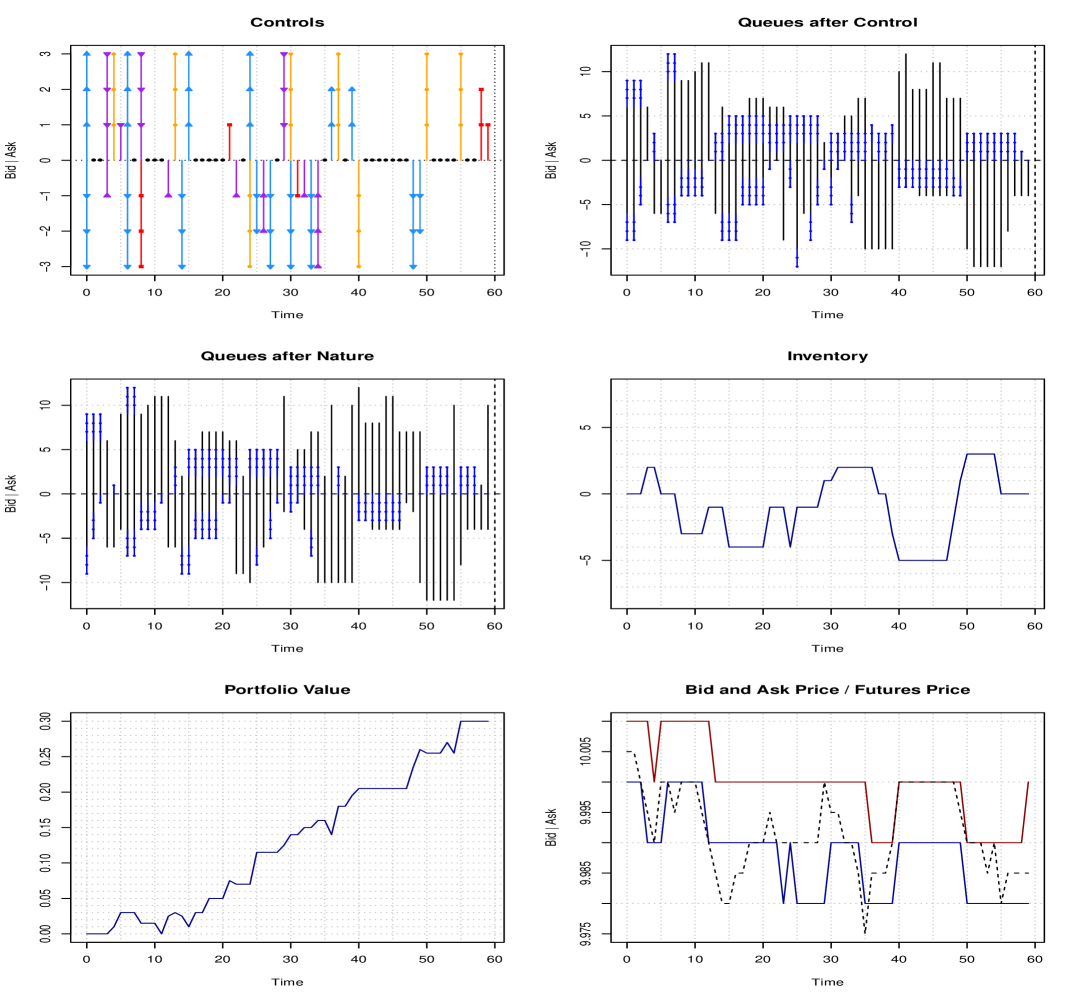
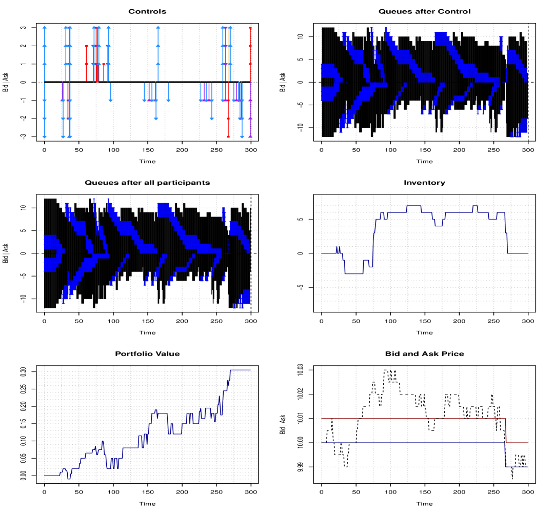
In Figure 2, we provide a simulated path of the optimal strategy, starting from a symmetric configuration of the order book, with queue lengths equal to $6$. In this simulation, the MM always play before the other (random) players. The top left graphic describes the control played by the MM. Triangles pointing outward (with respect to the zero line) correspond to limit orders, the number of triangles giving their size. Arrows with triangles pointing inward are cancellations, again the number of triangles gives the size. Aggressive orders are symbolized by lines with squares, while limit orders within the spread correspond to the lines with dots. The top right graphic gives the state of the order book just after the MM has played, and before the nature (i.e. the other players) plays. The size of the lines gives the total length of each queues, while the dots symbolize the position of the MM in the queue. The middle left graphic describes the state of the order book after the nature plays. The bottom left graphic gives the value of the portfolio of the MM if he had to liquidate (by sending aggressive orders) his stock holding at the best bid/ask price. The final value gives the “true” liquidation value of the book. In the case that the final inventory can not be liquidated at the best bid/ask price, we liquidate the remaining part at the best bid/ask price minus/plus one tick. The middle right graphic is the inventory just before he plays and the bottom right one is the bid and ask prices just after he plays. Figure 1 provides the distribution of the gain made by the MM, it uses $10^{5}$ simulated paths.

His strategy can seem difficult to interpret at first sight. But, we have to remember that he believes that the imbalance plays an important role in the book order dynamics, and that he not only should take care of it but that he can actually use it: some limit orders are sent not to be executed but to influence the evolution of the price in a favorable direction. Also note that he should avoid the price to go down/up if his inventory is positive/negative. Having this in mind, it is not surprising that he can be sometimes at the limit of a price manipulation strategy, if he is big enough with respect to the market, which is the case in these simulations. Finally, we have to keep in mind that his strategy is constrained. He sometimes cancels positions to be free to react more quickly to a more favorable market configuration later on.

Not surprisingly, the MM first sends limit orders of equal sizes on both sides of the order book. Nothing happens until time $t=9$. At this time is inventory is $2$ and his position at the ask is still far from the beginning of the queue. In order to avoid increasing again his inventory, he cancels his remaining position of one unit at the bid. He puts a new position at the bid at time $10$ after the queue has slightly increased, because of an exogenous limit order. Unfortunately for him, this new position is immediately executed, and his inventory jumps to $5$. After the queue is regenerated, he immediately puts a limit order of size $2$ at the bid. His reasoning is the following: 1. this position has little chance to be executed immediately, he does not take a risk of again increasing his inventory; 2. by doing this he increases the imbalance and therefore the probability of being executed at the ask so has to gain the spread and reduce his inventory. This strategy is successful since immediately $2$ units of his positions at the ask are executed. The imbalance is still good even if he cancels his last unit at the bid, so as to be free to play the control he wants once his last unit at the ask will be executed. In fact, it does not work and he decides to refresh his global position at time $16$ by canceling his final unit at the ask and putting limit orders again at time $17$ in a symmetric way. This is a limit spread order at the bid. This makes sense since he has to avoid the stock price to go down, because he has a positive inventory. The fact that just after he alternates between putting and canceling limit orders at the ask is probably a numerical artifact: on the one hand, he wants to have a limit position at the ask because his inventory is large, on the other hand he does not want to increase the imbalance to avoid having a too big probability of being executed at the bid and of seeing the price go down. Similarly, he wants to keep a position at the bid to avoid a downward price move, while he really does not want to be executed on this side. The aggressive order at the bid at time $19$ is just a partial cancellation, that is completed at time $20$. He just does not want to be executed. By doing so, he unfortunately causes a downward jump of the bid, which is not good for him. Just after he sends a limit spread order at the bid to fight against this downward pressure, and then cancels it once the bid is back at a distance one tick of the ask. This strategy is successful. The rest of his orders can be interpreted in a similar manner. Just note that he starts to be aggressive at the bid side at time $49$ because his inventory is too big and the maturity starts to be quite close, in particular the first market order of size $3$ compensates the execution of a position of size $3$ at the bid just before (so that the graphic of the inventory does not move, although the inventory temporary jumps to the upper limit $7$).

Figure 1: Density estimation of the gain made by the Market Maker.

Figure 2: Simulated path of the optimal strategy of the Market Maker.

4 High frequency trader’s pair trading problem

We now turn to the HFT strategy. We consider a pair trading strategy where the trader invests in the difference of two highly correlated assets. Here, we choose the futures price of the stock to be the second asset. The order book defined in Section 2 represents the dynamics of the stock. Whenever the trader buys/sells $n$ units of stocks (being by an aggressive order or by the execution of a limit order), she sells/buys immediately $n$ units of the futures. Her inventory should be fully liquidated at $T$.

4.1 The optimal control problem

We assume that the reference price $F$ of the futures is given by

$$F=\frac{P^{\mathfrak{b}}+P^{\mathfrak{a}}}{2}+S$$ (4.1)

where $S$ is a mean-reverting process

$$S=S_{0}+\int_{0}^{\cdot}\rho(\hat{s}-S_{t})dt+\int_{0}^{\cdot}\sigma(S_{t})dW_{t}.$$ (4.2)

Here, $\rho$ is the strength of mean reversion, $\hat{s}$ is the average of mean reversion and $\sigma:\mathbb{R}\mapsto\mathbb{R}$ is a Lipschitz bounded function representing the volatility of the process. In the following, we shall assume that

the support of $$\sigma$$ is bounded. (4.3)

Remark 4.1.

The above implies in particular that $S$ lies in a certain compact set $D_{S}$ as soon as $S_{0}$ does. This could clearly be relaxed to the price of a finer analysis.

The strategy of the HFT is described by the same quantities as the one of the MM in Section 3. The only difference lies in the fact that she constantly holds a number equal to $-I$ units of the futures $F$. We assume that buying/selling the futures leads to the payment of a proportional cost $\kappa\geq 0$. Then, the dynamics of the corresponding state process $X$ is given by

$$X_{\tau_{i}}={\cal T}_{X}(S_{\tau_{i}},P_{\tau_{i-1}},Q_{\tau_{i-1}},X_{\tau_{i-1}},\Delta{\cal E}^{\phi}_{\tau_{i}}){\bf 1}_{\{\Delta{\cal E}^{\phi}_{\tau_{i}}\neq 0\}}+\tilde{\cal T}_{X}(S_{\tau_{i}},P_{\tau_{i-1}},Q_{\tau_{i-1}},X_{\tau_{i-1}},\Delta\tilde{\cal E}_{\tau_{i}}){\bf 1}_{\{\Delta{\cal E}^{\phi}_{\tau_{i}}=0\}},$$ (4.4)

with ${\cal T}_{X}$ and $\tilde{\cal T}_{X}$ now defined with respect to

$${\cal T}_{G}(s,p,q,x,\delta)=g+(a^{\mathfrak{b}}-{\rm exe}(a^{\mathfrak{b}},n^{\mathfrak{b}},b^{\mathfrak{b}}))\Delta^{\mathfrak{b}}_{-}-(a^{\mathfrak{a}}-{\rm exe}(a^{\mathfrak{a}},n^{\mathfrak{a}},b^{\mathfrak{a}}))\Delta^{\mathfrak{a}}_{+}$$

$${\cal T}_{I}(s,p,q,x,\delta)=i-(a^{\mathfrak{b}}-{\rm exe}(a^{\mathfrak{b}},n^{\mathfrak{b}},b^{\mathfrak{b}}))+(a^{\mathfrak{a}}-{\rm exe}(a^{\mathfrak{a}},n^{\mathfrak{a}},b^{\mathfrak{a}}))$$

$${\cal T}_{N^{\mathfrak{b}/\mathfrak{a}}}(s,p,q,x,\delta)=n^{\mathfrak{b}/\mathfrak{a}}+[\ell^{\mathfrak{b}/\mathfrak{a}}-n^{\mathfrak{b}/\mathfrak{a}}]^{+}+\ell^{\mathfrak{b}/\mathfrak{a},\frac{1}{2}}-m^{\mathfrak{b}/\mathfrak{a}}-{\rm exe}(a^{\mathfrak{b}/\mathfrak{a}},n^{\mathfrak{b}/\mathfrak{a}},b^{\mathfrak{b}/\mathfrak{a}})$$

$${\cal T}_{B^{\mathfrak{b}/\mathfrak{a}}}(p,q,x,\delta)=b^{\mathfrak{b}/\mathfrak{a}}+(q^{\mathfrak{b}/\mathfrak{a}}-b^{\mathfrak{b}/\mathfrak{a}}){\bf 1}_{\{\ell^{\mathfrak{b}/\mathfrak{a}}\neq 0\}}-b^{\mathfrak{b}/\mathfrak{a}}{\bf 1}_{\{m^{\mathfrak{b}/\mathfrak{a}}=n^{\mathfrak{b}/\mathfrak{a}}\}}-(b^{\mathfrak{b}/\mathfrak{a}}\wedge a^{\mathfrak{b}/\mathfrak{a}}){\bf 1}_{\{a^{\mathfrak{b}/\mathfrak{a}}\neq 0\}}-b^{\mathfrak{b}/\mathfrak{a}}{\bf 1}_{\{\ell^{\mathfrak{b}/\mathfrak{a}}\neq 0\}}$$

$${\cal T}_{J}(s,p,q,x,\delta)=j+1$$

and

$$\tilde{\cal T}_{G}(s,p,q,x,\delta)=g-{\rm exe}(a^{\mathfrak{b}},n^{\mathfrak{b}},b^{\mathfrak{b}})\Delta^{\mathfrak{b}}_{+}+{\rm exe}(a^{\mathfrak{a}},n^{\mathfrak{a}},b^{\mathfrak{a}})\Delta^{\mathfrak{a}}_{-}$$

$$\tilde{\cal T}_{I}(s,p,q,x,\delta)=i+{\rm exe}(a^{\mathfrak{b}},n^{\mathfrak{b}},b^{\mathfrak{b}})-{\rm exe}(a^{\mathfrak{a}},n^{\mathfrak{a}},b^{\mathfrak{a}})$$

$$\tilde{\cal T}_{N^{\mathfrak{b}/\mathfrak{a}}}(s,p,q,x,\delta)=n^{\mathfrak{b}/\mathfrak{a}}-{\rm exe}(a^{\mathfrak{b}/\mathfrak{a}},n^{\mathfrak{b}/\mathfrak{a}},b^{\mathfrak{b}/\mathfrak{a}})$$

$$\tilde{\cal T}_{B^{\mathfrak{b}/\mathfrak{a}}}(p,q,x,\delta)=[b^{\mathfrak{b}/\mathfrak{a}}-a^{\mathfrak{b}/\mathfrak{a}}]^{+}{\bf 1}_{\{m^{\mathfrak{b}/\mathfrak{a}}=0\}}+(b^{\mathfrak{b}/\mathfrak{a}}-[m^{\mathfrak{b}/\mathfrak{a}}-(q^{\mathfrak{b}/\mathfrak{a}}-b^{\mathfrak{b}/\mathfrak{a}}-n^{\mathfrak{b}/\mathfrak{a}})]^{+})^{+}{\bf 1}_{\{m^{\mathfrak{b}/\mathfrak{a}}\neq 0\}}$$

$$\tilde{\cal T}_{J}(s,p,q,x,\delta)=0,$$

in which

$$\Delta^{\mathfrak{b}}_{\pm}:=p^{\mathfrak{b}}-\frac{p^{\mathfrak{b}}+p^{\mathfrak{a}}}{2}-s\pm\kappa\mbox{ , }\Delta^{\mathfrak{a}}_{\pm}:=p^{\mathfrak{a}}-\frac{p^{\mathfrak{b}}+p^{\mathfrak{a}}}{2}-s\pm\kappa.$$

In the above, we used the notations $x=(g,i,n^{\mathfrak{b}},n^{\mathfrak{a}},b^{\mathfrak{b}},b^{\mathfrak{a}},j)$, $\delta=(a^{\mathfrak{b}},a^{\mathfrak{a}},\ell^{\mathfrak{b}},\ell^{\mathfrak{a}},\ell^{\mathfrak{b},\frac{1}{2}},\ell^{\mathfrak{a},\frac{1}{2}},m^{\mathfrak{b}},$ $m^{\mathfrak{a}},$ $\varepsilon,\varepsilon^{\mathfrak{b}},\varepsilon^{\mathfrak{a}})$, $p=(p^{\mathfrak{b}},p^{\mathfrak{a}})$ and $q=(q^{\mathfrak{b}},q^{\mathfrak{a}})$.

The set of admissible controls ${\cal C}(0,S_{0},Z_{0-})$ is defined as in Section 3 but with respect to the (completed) filtration $\mathbb{F}^{\phi}=({\cal F}^{\phi}_{t})_{t\geq 0}$ generated by $(S,{\cal E})$.

We also assume that she has an exponential type utility function, with risk aversion parameter $\eta>0$. Then, she wants to maximize over $\phi\in{\cal C}(0,S_{0},Z_{0-})$ the expected utility

$$\mathbb{E}[U(S_{T},Z_{T}^{\phi})]$$

where

$$U(s,z):=-\exp\left(-\eta\{g+i^{+}\Delta^{\mathfrak{b}}_{-}-i^{-}{\Delta^{\mathfrak{a}}_{+}}-\kappa([i^{+}-q^{\mathfrak{b}}]^{+}+[i^{-}-q^{\mathfrak{a}}]^{+})-\varrho j\}\right)$$ (4.5)

for $z=(p^{\mathfrak{b}},p^{\mathfrak{a}},q^{\mathfrak{b}},q^{\mathfrak{a}},g,i,n^{\mathfrak{b}},n^{\mathfrak{a}},b^{\mathfrak{b}},b^{\mathfrak{a}},j)$, and where $\Delta^{\mathfrak{b}}_{\pm}$ and $\Delta^{\mathfrak{a}}_{\pm}$ are defined as above.

As in Section 3, we next extend the definition of our state processes by writing

$$(S^{t,s},Z^{t,s,z,\phi})=(S^{t,s},P^{t,s,z,\phi},Q^{t,s,z,\phi},X^{t,s,z,\phi})$$

for the process satisfying (2.12)-(3.1)-(4.2) for the control $\phi$ and the initial condition $(S^{t,s}_{t},Z^{t,s,z,\phi}_{t-})$ $=$ $(s,z)\in D_{S}\times D_{Z}$. The corresponding set of admissible controls is ${\cal C}(t,s,z)$, and the filtration associated to $\phi\in{\cal C}(t,s,z)$ is $\mathbb{F}^{t,s,z,\phi}=({\cal F}^{t,s,z,\phi}_{s})_{s\in[t,T]}$. We finally define the value function

$${\rm v}(t,s,z):=\sup_{\phi\in{\cal C}(t,s,z)}J(t,s,z;\phi)\;\mbox{ for }(t,s,z)\in[0,T]\times D_{S}\times D_{Z},$$

where

$$J(t,s,z;\phi):=\mathbb{E}[U(S^{t,s}_{T},Z^{t,s,z,\phi}_{T})].$$

We close this section with Remarks that are the counterparts of Remarks 3.2 and 3.3.

Remark 4.2.

For later use, observe that

$${\rm v}(t,s,z)=e^{-\eta(g-\varrho j)}\bar{\rm v}(t,z):=e^{-\eta(g-\varrho j)}{\rm v}(t,s,p^{\mathfrak{b}},p^{\mathfrak{a}},q^{\mathfrak{b}},q^{\mathfrak{a}},0,i,n^{\mathfrak{b}},n^{\mathfrak{a}},b^{\mathfrak{b}},b^{\mathfrak{a}},0)$$

for all $t\leq T$, $s\in D_{S}$ and $z=(p^{\mathfrak{b}},p^{\mathfrak{a}},q^{\mathfrak{b}},q^{\mathfrak{a}},g,i,n^{\mathfrak{b}},n^{\mathfrak{a}},b^{\mathfrak{b}},b^{\mathfrak{a}},j)\in D_{Z}$.

Remark 4.3.

Note that ${\rm v}$ is bounded from above by $0$ by definition. It also follows from (4.3) that $S^{t,s}$ takes values in the compact set $D_{S}$ so that ${\rm v}\in{\mathbf{L}}^{\rm exp}_{\infty}$ by the same reasoning as in Remark 3.3.

4.2 The dynamic programming equation

As in Section 3.3, we first provide a dynamic programming principle. Again, we let ${\rm v}_{*}$ and ${\rm v}^{*}$ denote the lower- and upper-semicontinuous envelopes of ${\rm v}$.

Proposition 4.1.

Fix $(t,s,z)\in[0,T]\times D_{S}\times D_{Z}$ and a family $\{\theta^{\phi},\phi\in{\cal C}(t,s,z)\}$ such that each $\theta^{\phi}$ is a $[t,T]$-valued $\mathbb{F}^{t,s,z,\phi}$-stopping time and $\|(S^{t,s}_{\theta^{\phi}},Z^{t,s,z,\phi}_{\theta^{\phi}})\|_{\infty}<\infty$. Then,

$$\sup_{\phi\in{\cal C}(t,x,q)}\mathbb{E}\left[{\rm v}_{*}(\theta^{\phi},S^{t,s}_{\theta^{\phi}},Z^{t,s,z,\phi}_{\theta^{\phi}})\right]\leq{\rm v}(t,s,z)\leq\sup_{\phi\in{\cal C}(t,x,q)}\mathbb{E}\left[{\rm v}^{*}(\theta^{\phi},S^{t,s}_{\theta^{\phi}},Z^{t,s,z,\phi}_{\theta^{\phi}})\right].$$

Proof. Let ${\cal C}_{k}(t,x,z)$ be the set of controls $\phi$ satisfying the additional constraint $\#\{\tau^{\phi}_{i},i\geq 1\}\leq k$ a.s., and let ${\rm v}_{k}$ be the corresponding value function, for $k\geq 1$. Then, it is not difficult to see that ${\rm v}_{k}$ is continuous, and the arguments of [10] imply that

$$\sup_{\phi\in{\cal C}_{k}(t,x,z)}\mathbb{E}\left[{\rm v}_{k}(\theta^{\phi},S^{t,s}_{\theta^{\phi}},Z^{t,s,z,\phi}_{\theta^{\phi}})\right] \leq{\rm v}_{k}(t,s,z)$$

$$\leq\sup_{\phi\in{\cal C}_{k}(t,x,z)}\mathbb{E}\left[{\rm v}_{k}(\theta^{\phi},S^{t,s}_{\theta^{\phi}},Z^{t,s,z,\phi}_{\theta^{\phi}})\right]$$

$$\leq\sup_{\phi\in{\cal C}(t,x,z)}\mathbb{E}\left[{\rm v}(\theta^{\phi},S^{t,s}_{\theta^{\phi}},Z^{t,s,z,\phi}_{\theta^{\phi}})\right].$$

Since by definition ${\rm v}=\lim_{k\to\infty}\uparrow{\rm v}_{k}$ and ${\cal C}(t,x,z)=\cup_{k\geq 1}{\cal C}_{k}(t,x,z)$, sending $k\to\infty$ in the above leads to the required result, recall Remark 4.3. $\Box$

The partial differential equation associated to ${\rm v}$ is then at least formally given by

$$\min\left\{-{\cal L}\varphi-{\cal I}\varphi,\varphi-{\mathcal{K}}\varphi\right\} =0\text{ on }[0,T)\times D_{S}\times D_{Z}$$ (4.6)

$$\min\left\{\varphi-U,\varphi-{\mathcal{K}}\varphi\right\} =0\text{ on }\{T\}\times D_{S}\times D_{Z},$$

in which ${\cal L}$ is the Dynkin operator associated to (4.2):

$${\cal L}\varphi=\partial_{t}\varphi+\rho(\hat{s}-s)\partial_{s}\varphi+\frac{1}{2}\sigma^{2}\partial^{2}_{ss}\varphi.$$

To fully characterize the value function, we need the additional assumption, similar to Assumption 3.2.

Assumption 4.1.

There exists a Borel function $\psi\in C^{1,2}([0,T]\times D_{S}\times D_{Z})$ such that

1. $0\geq{\cal L}\psi+{\cal I}\psi$ on $[0,T)\times D_{S}\times D_{Z}$,

2. $\psi-{\mathcal{K}}\psi\geq\iota$ on $[0,T]\times D_{S}\times D_{Z}$ for some $\iota>0$,

3. $\psi\geq U$ on $\{T\}\times D_{S}\times D_{Z}$,

4. $\liminf\limits_{n\to\infty}(\psi/{\rm L})(t_{n},s_{n},z_{n})=\infty$ if $|z_{n}|\to\infty$ as $n\to\infty$, for all $(t_{n},s_{n},z_{n})_{n\geq 1}\subset[0,T]\times D_{S}\times D_{Z}$.

Theorem 4.1.

Let Assumption 3.1 hold. Then, ${\rm v}_{*}$ (resp. ${\rm v}^{*}$) is a viscosity supersolution (resp. subsolution) of (4.6). If moreover Assumption 4.1 holds, then ${\rm v}$ is continuous on $[0,T)\times D_{Z}$ and is the unique viscosity solution of (4.6), in the class ${\mathbf{L}}^{\rm exp}_{\infty}$.

Proof. In view of Proposition 4.1, the derivation of the viscosity super- and subsolution properties is very standard under Assumption 3.1, see e.g.  [10]. As for uniqueness, this follows from a comparison principle that can be proved in the class ${\mathbf{L}}^{\rm exp}_{\infty}$ by arguing as in the proof of Theorem 3.1. $\Box$

As for the MM problem, Assumption 4.1 is easily checked when $J_{\circ}<\infty$.

Remark 4.4.

If $J_{\circ}<\infty$ and the supports of $\lambda(\cdot|p,q,c)$ and $\gamma(\cdot|p,q)$ are bounded, uniformly in $(p,q,c)\in({\mathfrak{d}}\mathbb{Z})^{2}\times\mathbb{N}^{2}\times\mathbf{C}_{\circ}$, then the function $\psi$ defined in Remark 4.4 also satisfies the requirements of Assumption 4.1, for $r$ large enough.

4.3 Dimension reduction, symmetries and numerical resolution

As in Section 3.4, one can use specificities of the value function to reduce the complexity of the resolution of (4.6). First, the variable $(g,j)$ can be omitted, see Remark 4.2. Moreover, if Assumption 3.3 holds, then one easily checks that

$${\bar{\rm v}}(t,s,p^{\mathfrak{b}},p^{\mathfrak{b}}+2\delta p,q^{\mathfrak{b}},q^{\mathfrak{a}},0,i,n^{\mathfrak{b}},n^{\mathfrak{a}},b^{\mathfrak{b}},b^{\mathfrak{a}},0)$$

does not depend on $p^{\mathfrak{b}}$. The difference with the relation obtained in Section 3.4 is du to (4.1) and the fact that the HFT always hold a symmetric position in the stock and the futures (he is protected against evolutions of the mid-price). The other symmetry relations described in Section 3.4 do not hold because of the dependence on the process $S$.

Let us now turn to the definition of a numerical scheme for (4.6). Recall that, under Assumption 3.5, the operators ${\cal I}$ and ${\mathcal{K}}$ are explicit. Hence, the only required discretization is in time and in the variable $s$. We shall consider separately the diffusion part and the obstacle part of the PDE. More precisely, we fix a time and a space grid $\pi^{n}_{t}:=\{t^{n}_{i},i\leq n_{t}\}$ and $\pi^{n}_{s}:=\{s^{n}_{i},i\leq n_{s}\}$ where $t^{n}_{i}=iT/{n_{t}}$ for $i\leq n_{t}$ and $s^{n}_{i}=\underline{s}+i(\overline{s}-\underline{s})/{n_{s}}$, $i\leq{n_{s}}$. Here, $\underline{s}$ and $\overline{s}$ are such that $D_{S}=[\underline{s},\overline{s}]$, recall Remark 4.1, and $n:=(n_{t},n_{s})\in\mathbb{N}^{2}$. We next define the sequence of space domains $D_{Z}^{k}:=D_{Z}\cap[-k,k]^{11}$ for $k\geq 1$, and we let ${\rm v}^{k}_{n}$ be defined by

$${\rm v}^{k}_{n}=\max\left\{\check{\rm v}^{k}_{n},{\mathcal{K}}\check{\rm v}^{k}_{n}\right\}=0\mbox{ on }\pi^{n}_{t}\times\pi^{n}_{s}\times D_{Z}^{k},$$ (4.7)

$${\rm v}^{k}_{n}-U=0\text{ on }(\{T\}\times\pi^{n}_{s}\times D_{Z}^{k})\cup(\pi^{n}_{t}\times\pi^{n}_{s}\times(D_{Z}\setminus D_{Z}^{k})).$$

Here, for $i\leq n_{t}-1$ and $i^{\prime}\leq n_{s}$,

$$\check{\rm v}^{k}_{n}(t^{n}_{i},s^{n}_{i^{\prime}},\cdot)=\mathbb{E}[{\rm v}^{k}_{n}(t^{n}_{i+1},{\rm p}_{n}(S^{t^{n}_{i},s^{n}_{i^{\prime}}}_{t^{n}_{i+1}}),\cdot)]+\frac{T}{n}{\cal I}{\rm v}^{k}_{n}(t^{n}_{i+1},s^{n}_{i^{\prime}},\cdot),\mbox{ on }D_{Z}^{k},$$ (4.8)

where ${\rm p}_{n}$ is the left-hand side projection operator on $\pi^{n}_{s}$.

Note that the above numerical scheme is not fully explicit as it requires to compute conditional expectations. This can however be easily performed either by a finite difference scheme or by Monte-Carlo techniques in a very classical way. Note in particular that the randomness in these conditional expectations only comes from a one dimensional factor.

Proposition 4.2.

Let Assumptions 4.1 and 3.5 hold, then the sequence $({\rm v}^{k}_{n})_{n\geq 1}$ converges pointwise to ${\rm v}$ as $n_{t},n_{s},k\to\infty$.

Proof. Note that Assumption 4.1 ensures that comparison holds for (4.6) in the class ${\mathbf{L}}^{\rm exp}_{\infty}$, see e.g., [6, Proposition 5.1]. Thus, as for Proposition 3.2, the result is an easy consequence of the stability result of [7]. $\Box$

4.4 Approximate optimal controls

The optimal control can be numerically estimated as in Section 3.4. We first extend $({\rm v}^{k}_{n},\check{\rm v}^{k}_{n})$ to $\pi^{n}_{t}\times D_{S}\times D_{Z}$ by setting $({\rm v}^{k}_{n},\check{\rm v}^{k}_{n})(\cdot,s,\cdot):=({\rm v}^{k}_{n},\check{\rm v}^{k}_{n})(\cdot,{\rm p}_{n}(s),\cdot)$. Then, we choose a measurable map $\hat{c}_{n}^{k}(t^{n}_{i},\cdot)$ such that

$$\hat{c}_{n}^{k}(t^{n}_{i},\cdot)\in{\rm arg}\max\{{\mathcal{K}}^{c}\check{\rm v}^{k}_{n}(t^{h}_{i},s,\cdot),\;c\in\mathbf{C}(\cdot)\}\;,\;\mbox{ on }D_{S}\times D_{Z}^{k}$$

$$\hat{c}_{n}^{k}(t^{n}_{i},\cdot)=0\mbox{ on }D_{S}\times(D_{Z}\setminus D_{Z}^{k}),$$

and define the sequence of stopping times

$$\hat{\tau}^{n,k}_{j+1}:=\min\{t^{n}_{i}:i\geq 0,t^{n}_{i}>\hat{\tau}^{n,k}_{j},({\rm v}^{k}_{n}-{\mathcal{K}}^{\hat{c}_{n}^{k}}\check{\rm v}^{k}_{n}(t^{n}_{i},\cdot))(t^{n}_{i},S_{t^{n}_{i}},\hat{Z}_{t^{n}_{i}-})=0\},\;j\geq 0,$$

with $\hat{\tau}^{n,k}_{0}:={0-}$, and in which $\hat{Z}^{n,k}=(\hat{P}^{n,k},\hat{Q}^{n,k},\hat{X}^{n,k})$ is defined as in (3.2)-(4.2) for the initial condition $Z_{0-}$ and the control associated to $\hat{\phi}^{k}_{n}:=(\hat{\tau}^{n,k}_{i},\hat{c}_{n}^{k}(\hat{\tau}^{n,k}_{i},S_{\hat{\tau}^{n,k}_{i}},\hat{Z}^{n,k}_{\hat{\tau}^{n,k}_{i}-}))_{i\geq 1}$ in a Markovian way. Again, this provides a sequence of controls that is asymptotically optimal.

Proposition 4.3.

Let the conditions of Proposition 4.2 hold. Then,

$$\lim_{k\to\infty}\lim_{n_{t},n_{s}\to\infty}\mathbb{E}[U(S_{T},\hat{Z}^{n,k}_{T})]={\rm v}(0,S_{0},Z_{0-}),$$

in which the limit is taken along sequences $n$ such that $n_{t}^{2}n_{s}^{-1}\to 0$.

Proof. Let $\gamma(p,q):=\int d\beta(c|p,q)$ and recall that $\gamma$ is uniformly bounded by assumption. The family $\{({\rm v}^{k}_{n},\check{\rm v}^{k}_{n})/{\rm L}\}_{k,n\geq 1}$ is uniformly bounded, compare with Remark 4.3. Also note that $(s,z)\in{D_{S}}\times D_{Z}^{k}\mapsto U$ is $C_{k}$-Lipschitz, for some $C_{k}>0$ that only depends on $k$. By induction (recall that the component $s$ is projected on $\pi^{n}_{s}$),

$$|\check{\rm v}^{k}_{n}(\cdot,s,\cdot)-\check{\rm v}^{k}_{n}(\cdot,s^{\prime},\cdot)|\leq C^{\prime}_{k}[|s-s^{\prime}|+n_{t}O(n_{s}^{-1})],\mbox{ for all }s,s^{\prime}\in D_{S},\mbox{ on }D_{Z}^{k},$$

for some $C^{\prime}_{k}>0$ that does not depend on $n{\in\mathbb{N}^{2}}$. Since $S$ is $1/2$-Hölder in time in ${\mathbf{L}}_{2}$, together with Assumption 3.5, this implies that

$${\mathcal{K}}^{c}{\cal I}\check{\rm v}^{k}_{n}(t^{n}_{i+1},s^{n}_{i^{\prime}},z) ={\mathcal{K}}^{c}\mathbb{E}[{\cal I}\check{\rm v}^{k}_{n}(t^{n}_{i+1},S^{t^{n}_{i},s^{n}_{i^{\prime}}}_{t^{n}_{i+1}},z)]+O_{k}(n_{t}^{-\frac{1}{2}})+n_{t}O_{k}(n_{s}^{-1}),$$

$$=\mathbb{E}[\check{\rm v}^{k}_{n}(t^{n}_{i+1},S^{t^{n}_{i},s^{n}_{i^{\prime}}}_{t^{n}_{i+1}},Z^{t^{n}_{i},z,c}_{t^{n}_{i+1}})]+O_{k}(n_{t}^{-\frac{1}{2}})+n_{t}O_{k}(n_{s}^{-1})\;\;\mbox{for $z\in D^{k}_{Z}$, $c\in\mathbf{C}(z)$,}$$

in which the exponent $c$ in $Z^{t^{n}_{i},z,c}$ means that the impulse $c$ is given at $t^{n}_{i}$, and we use Remark 2.1 again. In the above, $O_{k}(\xi)$ is a function, that may depend on $k$, but such that $\xi\in\mathbb{R}\setminus\{0\}\mapsto|O_{k}(\xi)|/\xi$ is bounded in a neighborhood of $0$. By the arguments already used in the proof of Proposition 3.3, it follows that

$${\rm v}^{k}_{n}(t^{n}_{i},s^{n}_{i^{\prime}},z)= \mathbb{E}[{\rm v}^{k}_{n}(t^{n}_{i+1},S^{t^{n}_{i},s^{n}_{i^{\prime}}}_{t^{n}_{i+1}},Z^{t^{n}_{i},z,0}_{t^{n}_{i+1}})]\vee\max_{c\in\mathbf{C}(z)}\mathbb{E}[{\rm v}^{k}_{n}(t^{n}_{i+1},S^{t^{n}_{i},s^{n}_{i^{\prime}}}_{t^{n}_{i+1}},Z^{t^{n}_{i},z,c}_{t^{n}_{i+1}})]$$

$$+o_{k}(n_{t}^{-1})+n_{t}O_{k}(n_{s}^{-1}),$$

and therefore

$${\rm v}^{k}_{n}(0,S_{0},Z_{0-}) =\mathbb{E}[U(S_{\theta^{n}_{k}},\hat{Z}^{n,k}_{\theta^{n}_{k}})]+o^{k}_{n}(1)+O_{k}(n_{t}^{2}n_{s}^{-1})$$

$$=\mathbb{E}[U(S_{T},\hat{Z}^{n,k}_{T})]+o^{k}_{n}(1)+O_{k}(n_{t}^{2}n_{s}^{-1})+o_{k}(1)$$

by induction, in which $o^{k}_{n}(1)$ goes to $0$ as $n\to\infty$, $o_{k}(1)$ goes to $0$ as $k\to\infty$, and $\theta^{n}_{k}$ is as in the proof of Proposition 3.3. It remains to appeal to Proposition 4.2. $\Box$

4.5 Numerical experiments

We use the same model as the one described in Section 3.6. As for the new parameters, we take $\hat{s}=0$, $\rho=50$ and $\sigma=0.2$, in particular the mean reversion parameter is taken to be large.

Figure 3: Simulated path of the optimal strategy of the High Frequency Trader.

We approximate the behavior of the spread process $S$ by a trinomial tree based on the transition probabilities associated to the diffusion (4.2), so that the expectation in (4.8) can be computed explicitly. More precisely, we consider a centered 6 points grid with mesh equal to half a tick (i.e. $0.005$).

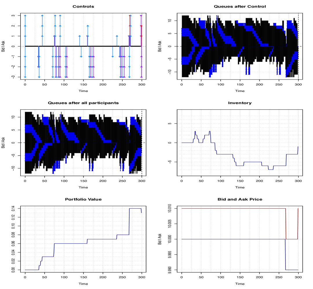
The graphics in Figure 3 have the same interpretation as in Section 3.6 except that we now also provide the evolution of the Futures process $F$, this is the dashed line in the bottom right graphic.
Remember that the HFT does not gain from the evolution of the mid-price, as her position in stocks in always covered by a symmetric position in the futures. She only gains from the evolution of the spread process $S$ or from the bid-ask spread of the stock if $S$ does not move. Not surprisingly, her behavior is quite different from the one of the MM described in Section 3.4.
As the MM would do, she first positions herself on the limits in a symmetric ways, because the spread with the future is $0$. She then tries selling at time $4$ by sending a limit sell order in the spread to buy the futures whose price (compared to the mid-price of the stock) is gone low. She is starting to play on the stock-futures spread. She follows this strategy until time $14$. She plays in a more symmetric way after this until time $35$, with a slight tendency to resume her inventory. At time $35$, she decides to clearly sell stocks again and buy the futures whose price is again very low. From time $40$ on, she inverts her position on the book to try buying the stock and thus sells the futures whose price has gown up. She finally inverts her position again at time $50$ when the futures price goes back to the mid price, to liquidate her position on the pair.
Compared to the positions of the MM in Figure 2, her positions in one direction are much more clear, and are clearly driven by the stock-futures spread. The HFT also does not seem to try to control the stock’s mid-price as the MM did, again this is because it does not matter for her.

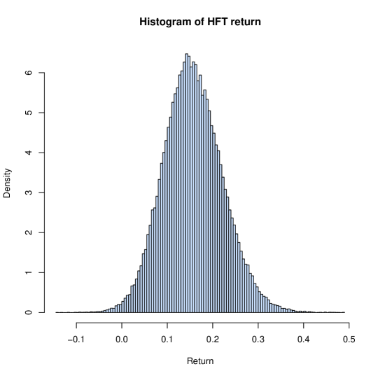
In Figure 4, we provide an estimation of the density of the gain of the HFT based on $10^{5}$ simulated paths.

Figure 4: Density estimation of the gain made by the High Frequency Trader.

5 Institutional broker strategies for portfolio liquidation

We now turn to the Institutional Broker problem. We consider in the following the two mostly used strategies for buying/selling a block of stocks. We focus on the buying side, selling being performed in a symmetrical way.

5.1 Volume strategy

We first consider a simple volume strategy. The aim of the broker is to buy ${\rm I_{0}}$ stocks. By convention, we set $I_{0}=-{\rm I}_{\circ}$. She fixes a participation rate $f\in(0,1)$. It corresponds to the percentage of the total volume of trades that should correspond to trades done by the broker between the initial time $0$ and the time at which the ${\rm I_{0}}$ stocks are bought. Therefore, she should buy $f/(1-f)$ of the total of the trades of the other market participant. To do so, she considers subintervals $[t_{i},t_{i+1}]$ of $\mathbb{R}_{+}$. At the beginning of each of this subintervals she estimates the conditional probability ${\rm p}_{i,i+1}$ that a trade arrives at the bid, given that a trade arrives and given the order book at $t_{i}$. Then, she puts a limit bid order of size $(f/(1-f))Q^{\mathfrak{b}}_{t_{i}}/{\rm p}_{i,i+1}$ at $t_{i}$. When all these units are executed, she adds new limit orders to keep her position to a level at least equal to $(f/(1-f))Q^{\mathfrak{b}}_{t_{i}}/{\rm p}_{i,i+1}$, or do nothing if this level is still achieved, and so on. In the meantime, she compares her realized volume $\Delta I:=I-I_{0}$ to the volume $\tilde{v}(0,\cdot)+\Delta I$ realized on the market from time $0$ on. Given a threshold $\delta_{I}>0$, she stops adding limit orders and cancels her orders already at the bid if $\Delta I(1-f)>f\tilde{v}(0,\cdot)+\delta_{I}$ and waits until $\Delta I(1-f)\leq f\tilde{v}(0,\cdot)+\delta_{I}$. If $\Delta I(1-f)<f\tilde{v}(0,\cdot)-\delta_{I}$, then she sends an aggressive order so as to turn to a position $\Delta I(1-f)\geq f\tilde{v}(0,\cdot)-\delta_{I}$ as soon as possible. She stops trading when $I\geq 0$.

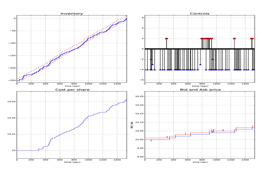
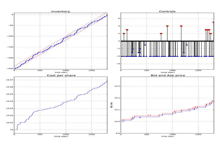
For our numerical experiment, we take the same model as in Section 3.6, we consider a participation rate $f=0.2$ and simply take ${{\rm p}_{i,i+1}=1/2}$. The time intervals $[t_{i},t_{i+1}]$ have a length of $60$ seconds and the time step is $1/2$ second. We take $\delta_{I}=4$ (i.e. $2$ ATS). The number of units to buy is ${\rm I}_{\circ}=250$ units. A simulated path of the strategy is provided in Figure 5. In the top left graphic, the dashed lines correspond to the target volume $\pm\delta_{I}$, while the solid curve is the volume traded by the IB. The top right graphic gives the control of the IB: lines with inward pointing arrows are limit orders, lines with squares are market orders. The bottom left graphic provides the evolution of the average price at which stocks have been bought by the IB from time $0$ on. The bottom right graphic gives the evolution of the bid and ask prices. One can see that this very simple strategy is quite efficient in the sense that only a limited number of market orders are sent. On the other hand, the systematic position of the IB at the bid limit creates an important imbalance that contributes to push up the price.

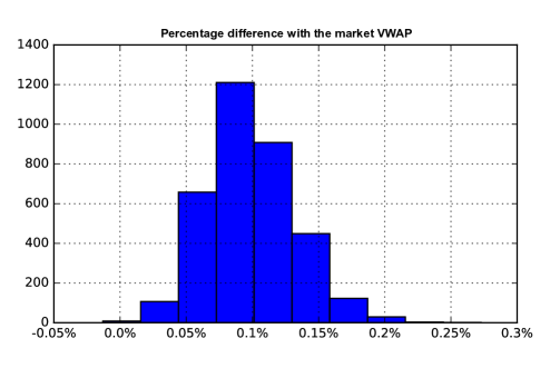
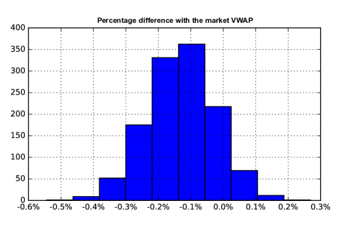
Figure 6 provides an histogram of the relative error (in $\%$) of the VWAP obtained by this strategy with respect to the VWAP realized at the level of the whole market. It is based on $10^{4}$ simulated paths. One can see that this average price is typically slightly higher than the VWAP of the market.

Figure 5: Simulated path of the volume strategy.

Figure 6: Histogram of the VWAP percentage error with respect to the VWAP of the market, for the Volume strategy.

5.2 VWAP

We now present a VWAP (Volume Weighted Average Price) based trading strategy frequently practiced by institutional brokers. Suppose that, at initial time $0$, an institutional broker decides to buy a quantity ${\rm I}_{0}\in\mathbb{N}$ of a tradable asset using a VWAP based strategy, i.e. by trying to obtain an average execution cost not more than

$$\text{VWAP}_{T}=\frac{{\rm w}_{T}}{v(0,T)}\;\mbox{ where }{\rm w}:=\int_{0}^{\cdot}v_{t}P_{t}dt\mbox{ and }v(\cdot,T):=\int_{\cdot}^{T}v_{s}ds,$$ (5.1)

in which $v$ is a deterministic non-negative continuous process such that $\int_{0}^{T}v_{t}dt>0$, which represents the trading volume of the market, and $P$ models the stock price.

5.2.1 Abstract continuous time resolution

Following the seminal work of Almgren and Chriss [4], see also [15, Section 4.4], we first consider the idealized world in which trading is done continuously at a bounded intensity, the trading speed $\vartheta$, taken as a process in the class ${\cal C}$ of non-negative processes adapted to the (completed) filtration generated by $W$. She assumes that the dynamics of the asset reference price $P$ has a permanent linear price impact generated by the agent’s trading activity, see [4]. More precisely, she assumes that the stock price evolves according to

$$dP_{t}=\beta\vartheta_{t}dt+\sigma dW_{t},$$ (5.2)

with $\beta,\sigma>0$, while her inventory $I$ follows the dynamics

$$dI_{t}=\vartheta_{t}dt$$

with the initial condition $I_{0}=-{\rm I}_{0}$, meaning that she is short at $0$ of the ${\rm I}_{0}$ stocks she has to buy on $[0,T]$.

She also assumes that her wealth $G$ is affected by a temporary linear market impact $\kappa\vartheta$, for some $\kappa>0$, i.e.

$$dG_{t}=-\vartheta_{t}\big{[}P_{t}+\kappa\vartheta_{t}\big{]}dt.$$ (5.3)

Her goal is to maximize over $\vartheta\in{\cal C}$ the expected utility

$$\mathbb{E}\left[-\exp[-\eta\{G_{T}+I_{T}(P_{T}-\tilde{\kappa}I_{T})-{\rm I}_{0}\frac{{\rm w}_{T}}{v(0,T)}\}]\right],$$ (5.4)

for some $\tilde{\kappa}>0$ which represents a penalty in case the inventory does not match $0$ at $T$.

This type of problems has been widely studied, see the book [15] for references. In the present form, it can be solved explicitly by using a verification argument based on the explicit solution of the Hamilton-Jacobi-Bellman equation corresponding to the value function $(t,p,i,g,w)\in[0,T]\times\mathbb{R}^{4}\mapsto{\rm v}(t,p,i,g,w)$ associated to the initial condition $(P_{t},I_{t},G_{t},{\rm w}_{t})=(t,p,i,g,w)$:

$$0=\sup_{u\geq 0}\left(\partial_{t}\varphi+\frac{1}{2}\sigma^{2}\partial^{2}_{pp}\varphi+pv_{t}\partial_{w}\varphi+u\left(\beta\partial_{p}\varphi+\partial_{i}\varphi-p\partial_{g}\varphi\right)-u^{2}\kappa\partial_{g}\varphi\right)\;\mbox{ on }[0,T)\times\mathbb{R}^{4}$$

with terminal condition

$$\varphi(T,p,i,g,w)=-e^{-\eta\{g+i(p-\tilde{\kappa}i)-\bar{m}_{0}w\}}\;\mbox{ for }(p,i,g,w)\in\mathbb{R}^{4},$$

where

$$\bar{m}:={\rm I}_{0}/v(0,T).$$

To simplify the above, we first write ${\rm v}$ is the form

$${\rm v}(t,p,i,g,w)=e^{-\eta(g-{\bar{m}}w-pv(t,T){\bar{m}})}\bar{\rm v}(t,p,i)\mbox{ with }\bar{\rm v}(t,p,i):={\rm v}(t,p,i,0,0),$$

so that $\bar{\rm v}$ formally solves

$$0=\partial_{t}\varphi+\frac{1}{2}\sigma^{2}(\partial^{2}_{pp}\varphi+2\eta v(t,T)\bar{m}\partial_{p}\varphi+\eta^{2}v(t,T)^{2}\bar{m}^{2}\varphi)-\frac{(\beta\partial_{p}\varphi+\beta\eta v(t,T)\bar{m}\varphi+\partial_{i}\varphi+\eta p\varphi)^{2}}{4\kappa\eta\varphi}$$

on $[0,T)\times\mathbb{R}^{4}$, with terminal condition

$$\varphi(T,p,i,g,w)=-e^{-\eta\{i(p-\tilde{\kappa}i)\}}\;\mbox{ for }(p,i,g,w)\in\mathbb{R}^{4}.$$

One possible solution is given by

$$\bar{\rm v}(t,p,i)=-e^{-\eta\{i(p-\tilde{\kappa}i)\}}e^{h_{0}(t)+h_{1}(t)i+h_{2}(t)i^{2}}$$

in which $h_{0},h_{1}$ and $h_{2}$ solve on $[0,T)$

$$\partial_{t}h_{0} =-\frac{1}{2}\sigma^{2}(\eta v(t,T)\bar{m})^{2}+\frac{(h_{1}+\beta\eta v(t,T)\bar{m})^{2}}{4\kappa\eta}$$

$$\partial_{t}h_{1} =\sigma^{2}\eta^{2}v(t,T)\bar{m}+(h_{1}+\beta\eta v(t,T)\bar{m})\frac{-\beta\eta+2\eta\tilde{\kappa}+2h_{2}}{2\kappa\eta}$$

$$\partial_{t}h_{2} =-\frac{\eta^{2}\sigma^{2}}{2}+\frac{\left[-\beta\eta+2\eta\tilde{\kappa}+2h_{2}\right]^{2}}{4\kappa\eta}$$

with $h_{0}(T)=h_{1}(T)=h_{2}(T)=0$. The solution of the last equation is of the form

$$h_{2}(t)=\frac{1}{c_{1}+c_{2}e^{c_{3}(T-t)}}-c_{4}$$

in which the constants $c_{1},\ldots,c_{4}$ can be computed explicitly by using the above differential equation and the terminal condition $h_{2}(T)=0$. Namely, set

$$a_{0}:=-\frac{\eta^{2}\sigma^{2}}{2}+\frac{\eta(2\tilde{\kappa}-\beta)^{2}}{4\kappa},\;a_{1}:=\frac{2\tilde{\kappa}-\beta}{\kappa},\;a_{2}=\frac{1}{\kappa\eta}$$

and let $y_{\circ}$ be a root of

$$(4a_{0}a_{2}-a_{1}^{2})y^{2}+(a_{1}^{2}-4a_{0}a_{2})y+a_{0}a_{2}=0,$$

then

$$c_{3}=\frac{a_{1}}{1-2y_{\circ}},\;c_{4}=\frac{a_{0}}{(1-y_{\circ})c_{3}},\;c_{1}=\frac{y_{\circ}}{c_{4}},\;c_{2}=\frac{1}{c_{4}}-c_{1}.$$

Existence of $y_{\circ}$ is guaranteed since

$$a_{1}^{2}-4a_{0}a_{2}=\frac{\eta^{2}\sigma^{2}}{2}>0.$$

Then, $h_{0}$ and $h_{1}$ are fully characterized.

An easy verification argument shows that this is actually the correct function and that the optimal control policy is given by

$$\hat{\vartheta}=\hat{v}(\cdot,I)$$

where

$$\hat{v}{(t,i)} :=\frac{\beta\partial_{p}{\rm v}(t,p,i,g,w)+\partial_{i}{\rm v}(t,p,i,g,w)-p\partial_{g}{\rm v}(t,p,i,g,w)}{2\kappa\partial_{g}{\rm v}(t,p,i,g,w)}$$

$$=\frac{\beta[i-v(t,T){\bar{m}}]-2\tilde{\kappa}i-[h_{1}(t)+2h_{2}(t)i]/\eta}{2\kappa}.$$

5.2.2 Strategy in practice and simulations

In practice, this optimal strategy can not be implemented within an order book. We therefore consider a “discrete” version. In this version, we assume that the IB tries to keep her inventory $I$ equal to the optimal inventory $\hat{I}:=\int_{0}^{\cdot}\hat{\vartheta}_{t}dt-{\rm I}_{\circ}$. To do this, she fixes a time grid $\{t_{i},i\leq n\}$ with $t_{0}=0$ and $t_{n}=T$. At time $t_{i}$, she estimates that she has to execute a volume of $V_{i,i+1}:=\int_{t_{i}}^{t_{i+1}}\hat{v}({t,I_{t_{i}}})dt$ on $[t_{i},t_{i+1}]$ while the volume of the market will be $\tilde{V}_{i,i+1}=\int_{t_{i}}^{t_{i+1}}v_{t}dt$. Then, she follows a volume strategy with threshold $\delta_{I}=+\infty$, see Section 5.1 above, on $[t_{i},t_{i+1}]$ with a target participation rate of $f=V_{i,i+1}/(\tilde{V}_{i,i+1}+V_{i,i+1})$. When $\Delta I:=I-I_{0}>\hat{I}+\bar{\delta}_{I}$, for some $\bar{\delta}_{I}>0$, orders are canceled and she waits until $\Delta I\leq\hat{I}+\bar{\delta}_{I}$. In the case where $\Delta I<\hat{I}-\bar{\delta}_{I}$, she puts market orders to reduce to the situation $\Delta I\geq\hat{I}-\bar{\delta}_{I}$ as soon as possible.

For our numerical experiment, we take the same configuration as in Section 5.1, with $\bar{\delta}_{I}={4}$, i.e.  ${2}$ ATS. The optimization of the VWAP strategy is done with a time horizon of $30$ minutes and a flat volume curve (so that the control does in fact not depend on it). The number of units to buy is ${\rm I}_{\circ}=250$ units. The additional parameters are set to $\eta=1$, $\sigma=0.2$, $\beta=0,0004$, $\kappa=0.003$ and $\tilde{\kappa}=\kappa*60$. The latter corresponds to the cost incurred when buying the remaining shares $I_{T}$ in $1$ additional minute after $T$, at a flat intensity in the theoretical continuous time model of Section 5.2.1. The volume intensity $v$ corresponds to $0.6$ ATS per second, i.e. $1.2$ units per second.

The interpretation of the different graphics in Figure 7 is the same as in Section 5.1, except that the dashed lines in the top left graphic correspond now to the optimal VWAP trading curve $\pm 2$ ATS. Again, we see that only a limited number of market orders were needed to be sent, but that the imbalance created by the VWAP trading algorithm drives the price up.

Figure 8 provides an histogram of the relative error (in $\%$) of the VWAP obtained by this strategy with respect to the VWAP of the whole market. It is based on $10^{4}$ simulated paths. One can see that he actually typically performs better than the market. Not surprisingly, this strategy performs better than the volume strategy in terms of VWAP.

Figure 7: Simulated path of the VWAP strategy.

Figure 8: Histogram of the percentage error with respect to the VWAP of the market, for the VWAP strategy.

6 Simulation of the full market

We now provide an illustration of possible interactions of several market participants. Again, a more realistic and general study is left for future research.

The prior and parameters of the participants are the same as the one that have been used in the above numerical experiments. More precisely, we consider one MM, one HFT and four IB. Among the IB, two are playing volume strategies (a buy and a sell) and two are playing WVAP strategies (a buy and a sell). At each time step, each participant decides of his optimal control given the current state of the order book. They send their orders at the same time. The control of the HFT is executed first, then this is the turn of the MM, and finally the controls of the Volume and VWAP trading algorithms are executed (we choose the order among them randomly, according to a uniform distribution). Since the MM and the Volume and VWAP trading algorithms decide before seeing the action of the HFT, their controls may not be applied or only partially, depending of the state of the order book after the previous participants have played. The exogenous randomness only comes from the simulation of the stock-futures spread process $S$ and from the new queues created when one queue is depleted. If the bid queue is depleted, then the bid price moves down. If the bid-ask spread is equal to two ticks, then the ask price moves down as well. The other way round if the ask queue is depleted. If the bid (resp. the ask) price moves down (resp. up), we consider that this is a discovered limit and its size is chosen as in Section 3.4: $10$ units with probability $60\%$, $5$ units with probability $25\%$ and $12$ units with probability $15\%$. If the bid (resp. the ask) price move up (resp. down), which can happen if the bid-ask spread is already of two ticks, we consider that this is a created limit and its size is chosen again as in Section 3.4: $2$ units with probability $60\%$, $1$ unit with probability $25\%$ and $3$ units with probability $15\%$. There is no other randomness, the rest of the dynamics is du to the HFT, the MM and the four other trading algorithms.

Note that only the VWAP trading algorithms are forced to trade, when they reach the (upper or lower) limit of their prescribed inventory path. In principle, the MM plays aggressive orders only when he needs to adjust quickly his inventory. For a typical path of the stock-futures spread, the HFT also has no incentive to send aggressive orders, except to adjust his inventory. Without trades, the Volume trading algorithms do not act as well (because the market volume does not move). Therefore, if the MM and the HFT have a zero initial inventory, we expect to have to wait for the VWAP trading algorithms to initiate first aggressive orders, and starts the whole dynamics.

In our illustration, we start with an initial state in which the HFT and the MM have a zero initial inventory. Each VWAP trading algorithm has to buy/sell 75 stocks within $5$ minutes of trading. This corresponds to an average of $0.5$ trades per second, which is consistent with the priors of the MM and the HFT.

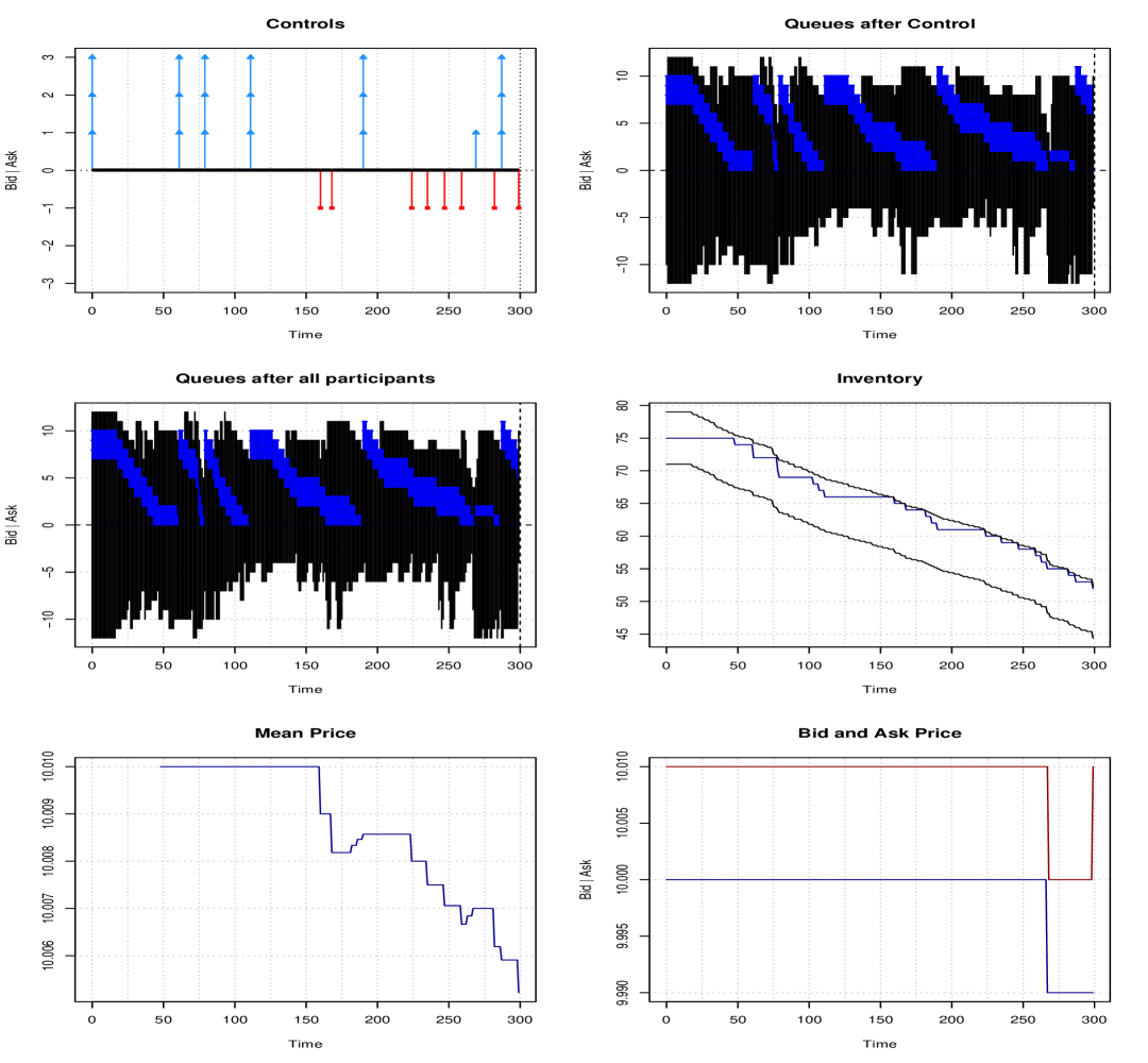
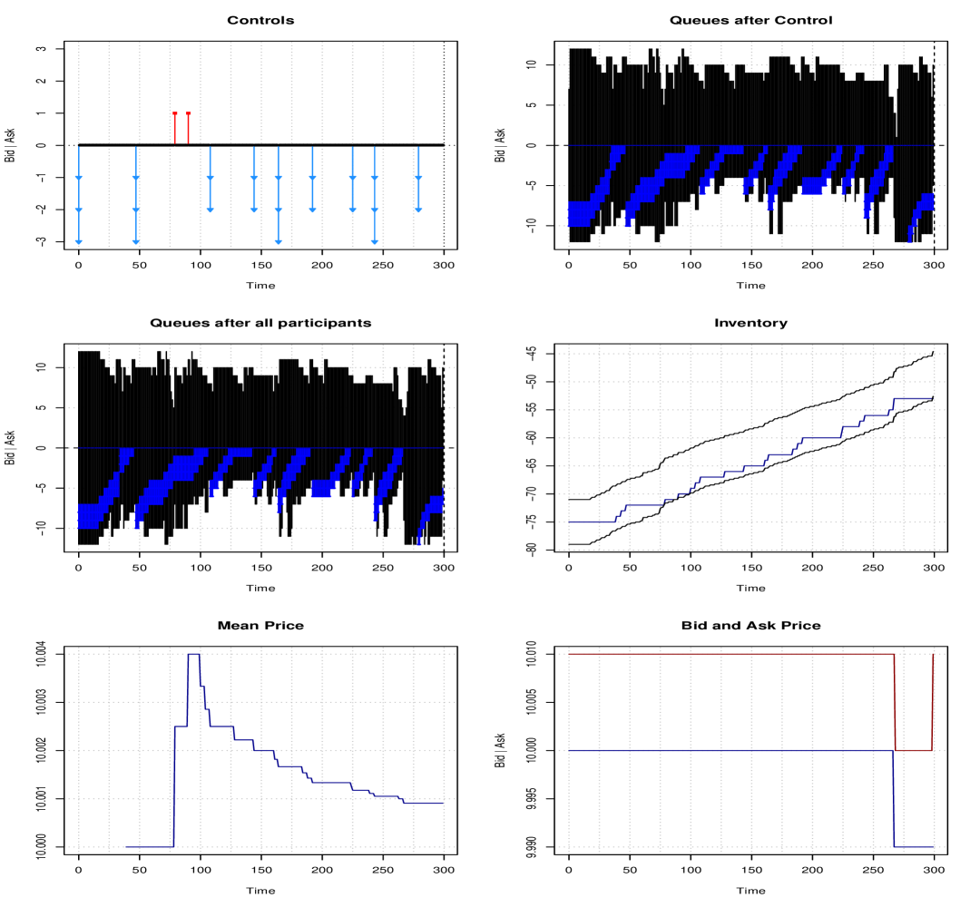
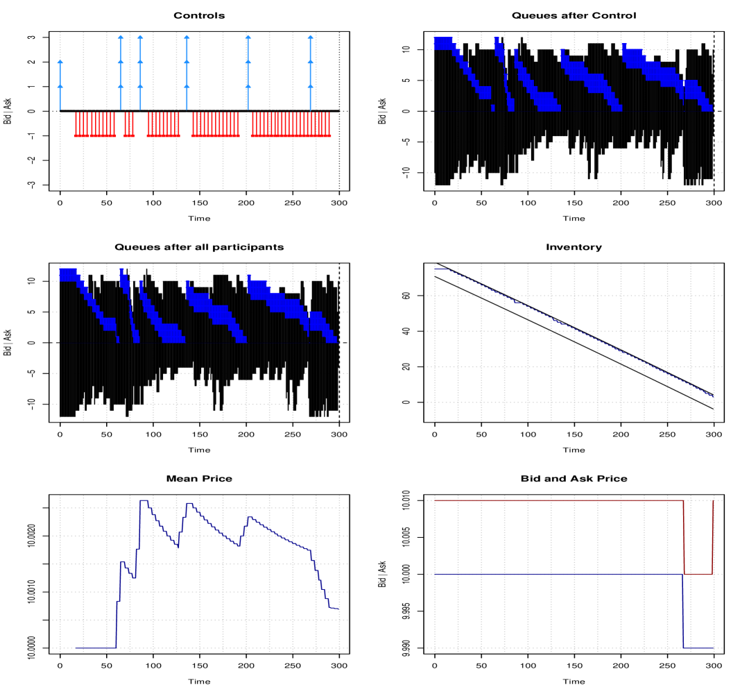
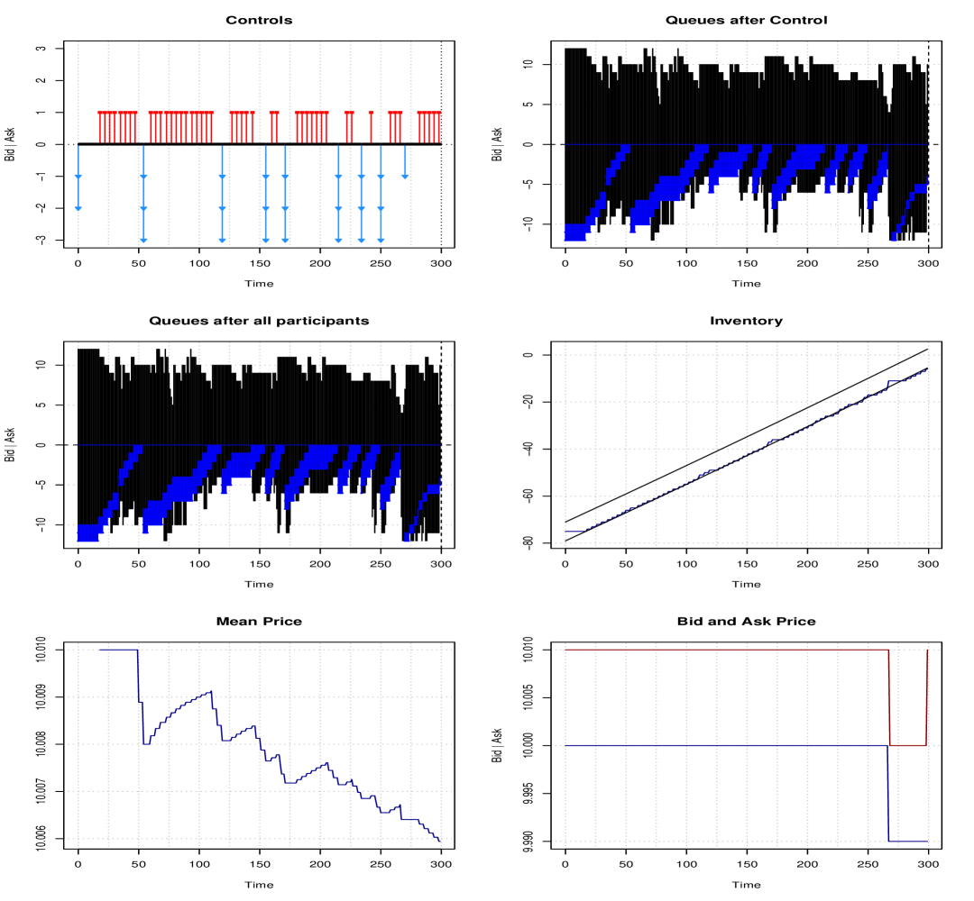
The Figures 9, 10, 11, 12, 13 and 14 have the same interpretation as in Section 3.4 except that now the position of the agent in the queue is in blue in the top right and middle left graphics (the black part corresponding to the other participants). The top right graphic is the state of the book just after the control of the agent is executed, the middle left is the state of the order book after the controls of all the participants have been executed. Note surprisingly, the trades are essentially due to the VWAP trading algorithms, to which the Volume trading algorithms need to adjust. The aggressive orders sent by the HFT and the MM are either cancellations or corrections of their inventory near the terminal time, except around time $35$ at which the HFT clearly wants to take a position on the stock-futures spread because it is very low. Note that the first price jump is due to an aggressive sell order of the HFT, slightly before time 275, which pushes the bid price down. He just after sends a limit sell order in the spread, and the ask price moves down as well. Since he is executed first and all players decide at the same time, he does not give to the others the opportunity to take this position in the spread. The last price move, just before $T$, is due to the HFT and the MM. This time the HFT and the MM send aggressive buy orders that deplete the queue (we do not see the price move on the graphics of the HFT, because they provide the prices after the execution of the order of the agent). As in Section 4.5, his position follows the stock-futures spread. In particular, between time 50 and 100, one can observe that he waits before sending a new sell limit order because the spread is gone up and he wants to buy stocks to short-sell the futures. When the spread starts going done, he takes a stronger position at the ask than at the bid, to start selling back the stock. As for the MM, he finishes with an inventory equal to $-1$, that will eventually be liquidated at $10.010$, which explains the downward jump of his portfolio value at $T$. When his inventory is very low, he balances between putting limit buy orders and letting the price go down by not supporting the bid limit. It is not successful until the price eventually moves down around time 275.

7 Conclusion

We have proposed a simplified but still realistic modeling of an order book, whose dynamics depends on the current imbalance. We have derived optimal strategies for three key actors: Market Makers, High Frequency Traders and Institutional Brokers (volume and VWAP trading algorithms). In this model, optimal strategies can be estimated numerically. Simulations show how complex optimal strategies are when actors believe that the imbalance actually has an impact on the dynamics of order flows. Our numerical simulations show that the construction of a realistic market simulator is feasible. A desirable next step would be to consider realistic proportions of market participants for the simulations proposed in Section 6 and to see whether the market statistics used to calibrate the different strategies can be retrieved through the simulated interactions of the various players. If this is the case, one can imagine trying to exhibit different market patterns depending on the nature and proportions of actors currently acting.

Acknowledgment: This research is part of a Cemracs 2017 project and benefited from the support of the Initiative de Recherche from Kepler-Chevreux and Collège de France. We are very grateful for the support of P. Besson and his team.

Figure 9: Optimal strategy of the High Frequency Trader when agents play together.

Figure 10: Optimal strategy of the Market Maker when agents play together.

Figure 11: Optimal strategy of the Volume trading algorithm (seller) when agents play together.

Figure 12: Optimal strategy of the Volume trading algorithm (buyer) when agents play together.

Figure 13: Optimal strategy of the VWAP trading algorithm (seller) when agents play together.

Figure 14: Optimal strategy of the VWAP trading algorithm (buyer) when agents play together.

References

- [1] Frédéric Abergel, Côme Huré, and Huyên Pham. Algorithmic trading in a microstructural limit order book model. arXiv preprint arXiv:1705.01446, 2017.
- [2] Frédéric Abergel and Aymen Jedidi. A mathematical approach to order book modeling. International Journal of Theoretical and Applied Finance, 16(05):1350025, 2013.
- [3] Frédéric Abergel and Aymen Jedidi. Long-time behavior of a hawkes process–based limit order book. SIAM Journal on Financial Mathematics, 6(1):1026–1043, 2015.
- [4] Robert Almgren and Neil Chriss. Value under liquidation. Risk, 12(12):61–63, 1999.
- [5] Nicolas Baradel, Bruno Bouchard, and Ngoc Minh Dang. Optimal trading with online parameter revisions. Market Microstructure and Liquidity, page 1750003, 2016.
- [6] Nicolas Baradel, Bruno Bouchard, and Ngoc Minh Dang. Optimal control under uncertainty and bayesian parameters adjustments. SIAM Journal on Control and Optimization, 56(2):1038–1057, 2018.
- [7] Guy Barles and Panagiotis E Souganidis. Convergence of approximation schemes for fully nonlinear second order equations. Asymptotic analysis, 4(3):271–283, 1991.
- [8] Christian Bayer, Ulrich Horst, Jinniao Qiu, et al. A functional limit theorem for limit order books with state dependent price dynamics. The Annals of Applied Probability, 27(5):2753–2806, 2017.
- [9] Paul Besson, Stéphanie Pelin, and Matthieu Lasnier. To cross or not to cross the spread: that is the question! The Journal of Trading, 11(4):77–91, 2016.
- [10] Bruno Bouchard and Nizar Touzi. Weak dynamic programming principle for viscosity solutions. SIAM Journal on Control and Optimization, 49(3):948–962, 2011.
- [11] Rama Cont and Adrien De Larrard. Order book dynamics in liquid markets: limit theorems and diffusion approximations. SSRN preprint 1757861, 2012.
- [12] Rama Cont and Adrien De Larrard. Price dynamics in a markovian limit order market. SIAM Journal on Financial Mathematics, 4(1):1–25, 2013.
- [13] Rama Cont, Sasha Stoikov, and Rishi Talreja. A stochastic model for order book dynamics. Operations research, 58(3):549–563, 2010.
- [14] Thierry Foucault. Order flow composition and trading costs in a dynamic limit order market1. Journal of Financial Markets, 2(2):99–134, 1999.
- [15] Olivier Guéant. The Financial Mathematics of Market Liquidity: From optimal execution to market making, volume 33. CRC Press, 2016.
- [16] Olivier Guéant. Optimal market making. Applied Mathematical Finance, 24(2):112–154, 2017.
- [17] Fabien Guilbaud and Huyen Pham. Optimal high-frequency trading with limit and market orders. Quantitative Finance, 13(1):79–94, 2013.
- [18] Weibing Huang, Charles-Albert Lehalle, and Mathieu Rosenbaum. Simulating and analyzing order book data: The queue-reactive model. Journal of the American Statistical Association, 10(509), December 2015.
- [19] Weibing Huang and Mathieu Rosenbaum. Ergodicity and diffusivity of markovian order book models: a general framework. SIAM Journal on Financial Mathematics, 8(1):874–900, 2017.
- [20] Aimé Lachapelle, Jean-Michel Lasry, Charles-Albert Lehalle, and Pierre-Louis Lions. Efficiency of the Price Formation Process in Presence of High Frequency Participants: a Mean Field Game analysis. Mathematics and Financial Economics, 10(3):223–262, June 2016.
- [21] Peter Lakner, Josh Reed, and Sasha Stoikov. High frequency asymptotics for the limit order book. Market Microstructure and Liquidity, 2(01):1650004, 2016.
- [22] Charles-Albert Lehalle and Othmane Mounjid. Limit order strategic placement with adverse selection risk and the role of latency. Market Microstructure and Liquidity, 3(01):1750009, 2017.
- [23] Charles-Albert Lehalle, Othmane Mounjid, and Mathieu Rosenbaum. Optimal liquidity-based trading tactics. arXiv preprint arXiv:1803.05690, 2018.
- [24] Christine A. Parlour. Price Dynamics in Limit Order Markets. The Review of Financial Studies, 11(4):789–816, 1998.
- [25] Ioanid Roşu. A dynamic model of the limit order book. Review of Financial studies, 22:4601–4641, 2009.
- [26] Eric Smith, Doyne J. Farmer, László Gillemot, and Supriya Krishnamurthy. Statistical Theory of the Continuous Double Auction. Quantitative Finance, 3(6):481–514, 2003.