A non-local linear dynamical system and violation of Bell’s inequality

Abstract A simple classical non-local dynamical system with random initial conditions and an output projecting the state variable on selected axes has been defined to mimic a two-channel quantum coincidence experiment. Non-locality is introduced by a parameter connecting the initial conditions to the selection of the projection axes. The statistics of the results shows violations up to 100$\%$ of the Bell’s inequality, in the form of Clauser-Horne-Shimony-Holt (CHSH), strongly depending on the non-locality parameter. Discussions on the parallelism with Bohmian mechanics are given.

1 Introduction

The Bell inequality [1] [2] is a milestone in the development of the post EPR [3] discussion on the completeness of Quantum Mechanics. The literature on the subject is huge and laboratory experiments confirm the violation of the inequality in the quantum world. Moreover, there are also several papers on the occurrence of Bell’s inequalities violation in classical random systems [4], [5], [6], [7], [8] . In this contest, the Accardi et al. papers, [9], [10] have raised an animate debate due mainly by Gill ( [11], [12] ). Usually, the experiments are based on computer randomness generation while in this paper we perform correlation experiments much possible close to the concept of the evolution of a dynamical state which resembles the causal Bohmian interpretation of EPR where initial conditions of the wave function appear to be crucial. In fact, the complete Bohm theory [13] is based on a deterministic dynamics and one could introduce randomness by randomizing the initial conditions according to the well known Born’s rule. So, the randomness of the quantum theory is due to our ignorance of initial conditions. The numerical experiment here proposed lies within these lines. In the first paragraph a simple two dimensional state-space dynamical system with a scalar output is defined. In the second paragraph we define the experiment which mimics the behavior of the quantum two-channel polarized photon experiment for testing the Clauser-Horne-Shimony-Holt (CHSH) inequality [14] . The third paragraph contains the set-up of the simulator and algorithm used to compute correlation among measurement pairs. The fourth paragraph presents the obtained results in terms of the statistics of the outputs. Finally, some conclusions and open questions are given.

2 The state-space linear system model

Consider the following two-dimensional linear dynamical system in the state-space representation:

$$\dot{X}=AX$$ (1)

$$Y=CX$$

$A=\begin{pmatrix}0&1\\ -1&0\end{pmatrix}$; $\hskip 28.45274ptC=\begin{bmatrix}\cos(\theta)&\sin(\theta)\end{bmatrix}$; $\hskip 28.45274ptX^{T}:=\begin{bmatrix}x_{1}&x_{2}\end{bmatrix}$

The formal solution for the state propagation starting with an initial condition: $X_{0}:=X(t=0)$ is:

$$X(t)=X_{0}e^{tA}$$ (2)

In this case, the solution is simply a sinusoidal wave. The output is the projection of the state vector along the axis defined by $\theta$:

$$y(t)=\begin{bmatrix}\cos(\theta)&\sin(\theta)\end{bmatrix}\begin{bmatrix}x_{1}(t)\\ x_{2}(t)\end{bmatrix}$$ (3)

3 The design of the experiment

The usual Alice and Bob perform separate measurements from the output $y$ of the system (1) at time $t=t_{1}$ by choosing independently an angle $\theta$.
The scheme is reported in Figure 1.

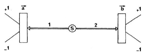
Figure 1: Scheme of the experiment: S can be considered as a source as well as the black box containing the system state

The results coming from Alice measurements are labeled with $\{a\}$ and those from Bob with $\{b\}$ .
In order to reproduce the typical measurements of a quantum system, we define the measurements in the set $\{-1,+1\}$ according to the following rule:

$$a_{i}=\operatorname{sign}[y_{a}(t=t_{1})](i=1,2)$$ (4)

$$b_{i}=\operatorname{sign}[y_{b}(t=t_{1})](i=1,2)$$

The idea is to test, by means of a series of experiments, whether it is possible to violate the Bell’s inequality by testing the experimental correlations defined in a standard way as:

$$E=(N_{++}+N_{--}-N_{+-}-N_{-+})/(N_{++}+N_{--}+N_{+-}+N_{-+})$$ (5)

Where: $N_{++}$ means that $(a=+1)\wedge(b=+1)$ and so on. Actually, being the experiment a typical two-channel experiment, the CHSH inequality in the following form is more suitable:

$$S=E(a_{1}b_{1})-E(a_{1}b_{2})+E(a_{2}b_{1})+E(a_{2}b_{2})\leqslant 2$$ (6)

Furthermore, the derivation of the original Bell inequality assumes perfect anticorrelation of entangled photon measurements in the EPR setup. The CHSH inequality has the reputation of being superior for all purposes. It is harder to violate and its derivation does not need anti-correlation. The following hypotheses are assumed to derive the CHSH inequality :

Hidden variables: The results of any measurement on any individual system are predetermined;

Non-Locality: It is well known that non-locality is necessary to reproduce the quantum mechanics in a deterministic context. So, non-local effect are here introduced in the initial conditions (hidden variables) by the following rule:

$$x_{1}(0)=r_{1}+\lambda\cos(\vartheta_{1});$$

$$x_{2}(0)=r_{2}+\lambda\cos(\vartheta_{2});$$

where: $r_{1}$ and $r_{2}$ are Gaussian random noises with $0$ mean and unitary variance; and $\lambda\cos(\vartheta_{1})$ and $\lambda\cos(\vartheta_{2})$ constitute the dependence of the initial conditions on the chosen angle by both Bob and Alice experimental setting. The violation of a Bell inequality guarantees that the observed outputs are not predetermined and that they arise from entangled quantum systems that possess intrinsic randomness. As for the standard tests for quantum systems, the experiments consist on four sub-experiments (each for any correlation pair) and the state model is the same both for Alice and Bob who do not know the system state and perform the measurements separately at the same time $t_{1}$. To randomize the system, the initial condition of the state variable $X_{0}$ is picked-up from a normal distribution with zero mean and unitary variance according to the non-local position described in the formula above in every run of each sub-experiment. To obtain a significant statistics, a large number of experiments have to be performed by iterating the procedure. In an algorithmic language, the process can be synthesized as follows:

Set $\lambda$
 For n=1,Nmax
 For i=1,M
 Do [random $X_{0}$, State propagation$\Rightarrow$ measurement $a_{1}$ and $b_{1}$]
 end
 Compute correlation according to (5)$E(a_{1}b_{1})$
 For i=1,M
 Do [random $X_{0}$, State propagation$\Rightarrow$ measurement $a_{1}$ and $b_{2}$]
 end
 Compute correlation $E(a_{1}b_{2})$
 For i=1,M
 Do [random $X_{0}$, State propagation$\Rightarrow$ measurement $a_{2}$ and $b_{1}$]
 end
 Compute correlation $E(a_{2}b_{1})$
 For i=1,M
 Do [random $X_{0}$, State propagation$\Rightarrow$ measurement $a_{2}$ and $b_{2}$]
 end
 Compute correlation $E(a_{2}b_{2})$
 Compute S(n)
 end
 Compute statistics on S

4 Running the model

We chose as angles for the coincidence measurements the ones which, according to the quantum theory, give $S=2\sqrt{2}$.

$$\{\theta\}=\{\dfrac{\pi}{2},0,\dfrac{\pi}{4},-\dfrac{\pi}{4}\}$$ (7)

The importance of this configuration lies on the fact that it corresponds to a situation which cannot be reproduced by a hidden variable theory. We have performed 100 (Nmax) independent runs with M=100 yielding hundred measurement pairs in each sub-experiment. The $Mathematica^{TM}$ software has been used for the simulations and for the statistical analyses of the outputs. In what follows, the measurement pairs with respect to the chosen angles are reported in details.

First coincidence measurements

$$a_{1}=\operatorname{sign}[y_{a}(t_{1})]=\begin{bmatrix}\cos(\dfrac{\pi}{2})&\sin(\dfrac{\pi}{2})\end{bmatrix}\begin{bmatrix}x_{1}(t_{1})\\ x_{2}(t_{1})\end{bmatrix}$$ (8)

$$b_{1}=\operatorname{sign}[y_{b}(t_{1})]=\begin{bmatrix}\cos(\dfrac{\pi}{4})&\sin(\dfrac{\pi}{4})\end{bmatrix}\begin{bmatrix}x_{1}(t_{1})\\ x_{2}(t_{1})\end{bmatrix}$$

Second coincidence measurements

$$a_{1}=\operatorname{sign}[y_{a}(t_{1})]=\begin{bmatrix}\cos(\dfrac{\pi}{2})&\sin(\dfrac{\pi}{2})\end{bmatrix}\begin{bmatrix}x_{1}(t_{1})\\ x_{2}(t_{1})\end{bmatrix}$$ (9)

$$b_{2}=\operatorname{sign}[y_{b}(t_{1})]=\begin{bmatrix}\cos(-\dfrac{\pi}{4})&\sin(-\dfrac{\pi}{4})\end{bmatrix}\begin{bmatrix}x_{1}(t_{1})\\ x_{2}(t_{1})\end{bmatrix}$$

Third coincidence measurements

$$a_{2}=\operatorname{sign}[y_{a}(t_{1})]=\begin{bmatrix}\cos(0)&\sin(0)\end{bmatrix}\begin{bmatrix}x_{1}(t_{1})\\ x_{2}(t_{1})\end{bmatrix}$$ (10)

$$b_{1}=\operatorname{sign}[y_{b}(t_{1})]=\begin{bmatrix}\cos(\dfrac{\pi}{4})&\sin(\dfrac{\pi}{4})\end{bmatrix}\begin{bmatrix}x_{1}(t_{1})\\ x_{2}(t_{1})\end{bmatrix}$$

Fourth coincidence measurements

$$a_{2}=\operatorname{sign}[y_{a}(t_{1})]=\begin{bmatrix}\cos(0)&\sin(0)\end{bmatrix}\begin{bmatrix}x_{1}(t_{1})\\ x_{2}(t_{1})\end{bmatrix}$$ (11)

$$b_{2}=\operatorname{sign}[y_{b}(t_{1})]=\begin{bmatrix}\cos(-\dfrac{\pi}{4})&\sin(-\dfrac{\pi}{4})\end{bmatrix}\begin{bmatrix}x_{1}(t_{1})\\ x_{2}(t_{1})\end{bmatrix}$$

4.1 Results: CHSH inequality violation

For each selected values of $0\leq\lambda\leq 10$ the process, as described above, has been run and the results obtained of the overall expected value of $S$ and on the percentage of CHSH violations and are reported in the Figures 2 and 3 respectively. By performing several runs, also by increasing the number M of measurements pairs and the number of iterations, the overall statistics do not show any significant variation.

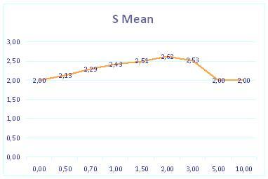
Figure 2: S mean values as a function of $\lambda$

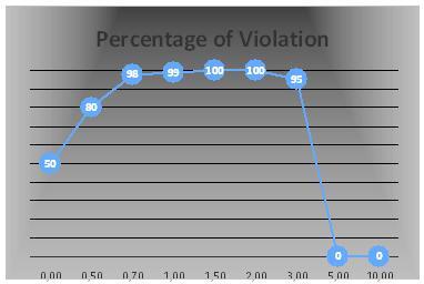
Figure 3: Percentage of violation as a function of $\lambda$

Furthermore, the following figures show the statistics of the run with $\lambda=2$ corresponding to the maximum value of the average of $S$ i.e. $\langle S\rangle=2.62$ with a standard deviation $STD(S)=0.12$. Note that this value is not to far from the quantum value $S=2\sqrt{2}\simeq 2.83$.

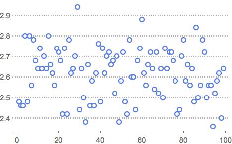
Figure 4: Iteration number and corresponding S value ($\lambda=2$)

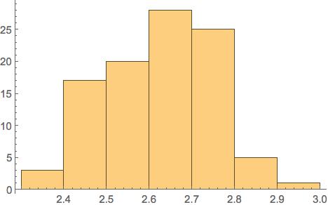
Figure 5: Histogram of the values of S violating the CHSH inequality ($\lambda=2$)

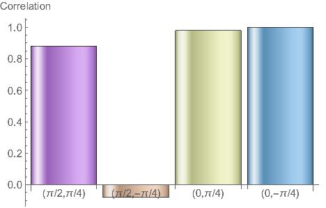
Figure 6: Correlation values of the maximal violation ($S=2.94$) of CHSH inequality ($\lambda=2$)

If we look to Fig. 2 and 3, we notice that for an experiment forced to locality i.e. $\lambda=0$, the expectation value is 2, and 50$\%$ of the runs violate the inequality. This is expected from the completely random nature of the output (Fig. 7). As the effect of non-locality affects the initial condition the violation is growing up to the maximum value for $S$ mean corresponding to $\lambda=2$. By further increasing $\lambda$ a decay on violation up to 0 percentage and again an average value of $S$ equal to 2 is obtained. This because the randomness of initial conditions are negligible and the system becomes a causal deterministic system yielding the upper limit of the CHSH inequality.

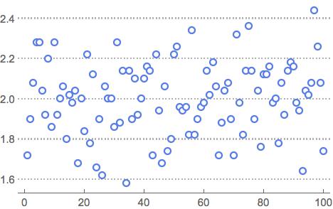
Figure 7: Iteration number and corresponding S value for $\lambda=0$

5 Conclusions

We do not want to force any ”philosophical” speculation on the results. It is well known that an impenetrable wall separating Quantum from Classical Mechanics does exist. We simply enumerate the following facts.
Coincidence measurements from a deterministic but non-local and simple linear dynamical model with random initial conditions show violations of the CHSH inequality up to hundred percent of coincidence measurements and the statistics of the results are robust against the large number of repeated experiments and the number of the measurement values. In the case of locality the results are in agreement with other random simulations. As Gill pointed out,: ”it is easy to make simulation models of local realistic loophole free CHSH-type experiments which violate CHSH i.e. the mean value of S is 2 and half the time the experiment gives a larger result and half the time it gives a smaller result” (https://pubpeer.com/publications /B087561066AD645C5348ADC2E4CF1C). The approach of our experiment is to mimic through a simple dynamical system some aspects of the Bohmian mechanics. Bohmian mechanics is a deterministic theory where a probabilistic element is introduced as probability is introduced into classical mechanics. The observer does not possess the full information about the true initial configuration of the system, but rather he has to retreat to a probability density. (See for example: [15] for a criticism of Bohmian theory). Of course, we cannot conclude that our results might imply adequacy or inadequacy of Bohmian point of view.

References

- [1] Bell, J. S.: On the Einstein Podolsky Rosen paradox. Physics(3), 195–200 (1964); reprinted in Bell,J.S. Speakable and Unspeakable in Quantum Mechanics. 2nd ed., Cambridge: Cambridge University.
- [2] Bell, J.S.: On the problem of hidden variables in quantum mechanics. Rev. Mod. Phys. 38, 447–452 (1966).
- [3] Einstein, A.; Podolsky, B.; Rosen, N.: Can Quantum-Mechanical Description of Physical Reality be Considered Complete? Phys. Rev. 47(10), 777-780 (1935).
- [4] Aerts, D., 1982, Example of a macroscopical situation that violates Bell inequalities”, Lett. Nuovo Cim., 34, 107.
- [5] Aerts, D. and Durt, T., 1994, Quantum. classical and intermediate, an illustrative example”, Found. Phys. 24, 1353 - 1368.
- [6] J. Kofler and C. Brukner, Conditions for Quantum Violation of Macroscopic Realism, Phys. Rev. Lett. 101, 090403 (2008).
- [7] Vongehr, S.: Quantum Randi Challenge and Didactic Randi Challenges arxiv.org/abs/1207.5294v3 (2012).
- [8] L. Clemente and J. Kofler, Necessary and sufficient conditions for macroscopic realism from quantum mechanics, Phys. Rev. A 91, 062103 (2015).
- [9] Luigi Accardi, Massimo Regoli:Locality and Bell’s inequality. Preprint Volterra, N. 427 (2000) quant-ph/0007005; an extended version of this paper, including the description of the present experimen will appear in the proceedings of the conference Foundations of Probability and Physics, Vaxjo University, Sweden, November 27 - December 1 (2000), A. Khrennikov (ed.), World Scientific (2001).
- [10] L.Accardi, K.Imafuku, M.Regoli: On the physical meaning of the EPR–chameleon experiment, Infinite dimensional analysis, quantum probability and related topics, 5 N. 1 (2002) 1–20; quant-ph/0112067.
- [11] Gill, R.D.: Time, Finite Statistics, and Bell’s Fifth Position. In Proc. of Foundation of Probability and Physics – 2 Ser. Math. Modelling in Phys., Engin. And Cogn. Sci, 5, (2002) pp. 179-206. Vaxjo Univ. Press, (2003).
- [12] Gill, R.D.; Larsson, J.A.: Accardi contra Bell (cum mundi): The impossible coupling. In Mathematical Statistics and Applications: Festschrift for Constance van Eeden. Eds: M. Moore, S. Froda and C. L’eger, pp. 133-154. IMS Lecture Notes, Monograph Series 42, Institute of Mathematical Statistics, Beachwood, Ohio (2003).
- [13] Bohm, D., 1951, Quantum Theory, Prentice-Hall, Englewood Cliffs, New York.
- [14] Clauser, J.F.; Horne, M.A.; Shimony, A.; Holt, R.A.: Proposed Experiment to Test Local Hidden-Variables Theories. Phys. Rev. Lett. 23, 880-884 (1969).
- [15] Kim Joris Bostrom, Is Bohmian Mechanics an empirically adequate theory? arXiv:1503.00201v2 [quant-ph] (2015).