Charged pion masses under strong magnetic fields in the NJL model

Abstract

The behavior of charged pion masses in the presence of a static uniform magnetic field is studied in the framework of the two-flavor NJL model, using a magnetic field-independent regularization scheme. Analytical calculations are carried out employing the Ritus eigenfunction method, which allows us to properly take into account the presence of Schwinger phases in the quark propagators. Numerical results are obtained for definite model parameters, comparing the predictions of the model with present lattice QCD results.

The study of the behavior of strongly interacting matter under intense external magnetic fields has gained increasing interest in the last few years Kharzeev:2012ph ; Andersen:2014xxa ; Miransky:2015ava , especially due to its applications to the analysis of relativistic heavy ion collisions HIC and the description of compact objects like magnetars duncan . From the theoretical point of view, addressing this subject requires to deal with quantum chromodynamics (QCD) in nonperturbative regimes, therefore, present analyses are based either in the predictions of effective models or in the results obtained through lattice QCD (LQCD) calculations. In this work we focus on the effect of an intense external magnetic field on $\pi$ meson properties. This issue has been studied in the last years following various theoretical approaches for low-energy QCD, such as Nambu-Jona-Lasinio (NJL)-like models Fayazbakhsh:2013cha ; Fayazbakhsh:2012vr ; Avancini:2015ady ; Zhang:2016qrl ; Avancini:2016fgq ; Mao:2017wmq ; GomezDumm:2017jij ; Wang:2017vtn ; Liu:2018zag , chiral perturbation theory Andersen:2012zc ; Agasian:2001ym and path integral Hamiltonians Orlovsky:2013wjd ; Andreichikov:2016ayj . In addition, results for the light meson spectrum under background magnetic fields have been recently obtained from LQCD calculations Bali:2011qj ; Hidaka:2012mz ; Luschevskaya:2014lga ; Bali:2015vua ; Bali:2017ian ; Bali:2017yku .

In the framework of the NJL model, mesons are usually described as quantum fluctuations in the random phase approximation (RPA) Vogl:1991qt ; Klevansky:1992qe ; Hatsuda:1994pi , that is, they are introduced via a summation of an infinite number of quark loops. In the presence of a magnetic field, the calculation of these loops requires some special care due to the appearance of Schwinger phases Schwinger:1951nm associated with each quark propagator. For the neutral pion these phases cancel out, and as a consequence the usual momentum basis can be used to diagonalize the corresponding polarization function Fayazbakhsh:2013cha ; Fayazbakhsh:2012vr ; Avancini:2015ady ; Avancini:2016fgq ; Mao:2017wmq . On the other hand, for the charged pions the Schwinger phases do not cancel, leading to a breakdown of translational invariance that prevents to proceed as in the neutral case. In this situation, some existing calculations Zhang:2016qrl ; Liu:2018zag just neglect the Schwinger phases, taking into account only the translational invariant part of the quark propagator. Very recently Wang:2017vtn , the use of the derivative expansion approach has been proposed as an improved approximation to deal with this issue. It should be noticed, however, that such an approach is expected to be less reliable as the mass of the meson and/or the magnetic field increase. The aim of the present work is to introduce a method that allows us to fully take into account the translational-breaking effects introduced by the Schwinger phases in the calculation of the charged meson masses in the RPA approach. Our method is based on the Ritus eigenfunction approach Ritus:1978cj to magnetized relativistic systems, which, as we show below, allows us to fully diagonalize the charged pion polarization function.

We start by considering the Euclidean Lagrangian density for the NJL two-flavor model in the presence of an electromagnetic field. One has

$${\cal L}\ =\ \bar{\psi}\left(-i\,\hbox to0.0pt{/\hss}\!D+m_{0}\right)\psi-G\left[(\bar{\psi}\,\psi)^{2}+(\bar{\psi}\,i\gamma_{5}\vec{\tau}\,\psi)\right]\ ,$$ (1)

where $\psi=(u\ d)^{T}$, $\tau_{i}$ are the Pauli matrices, and $m_{0}$ is the current quark mass, which is assumed to be equal for $u$ and $d$ quarks. The interaction between the fermions and the electromagnetic field ${\cal A}_{\mu}$ is driven by the covariant derivative

$$D_{\mu}\ =\ \partial_{\mu}-i\,\hat{Q}\mathcal{A}_{\mu}\ ,$$ (2)

where $\hat{Q}=\mbox{diag}(q_{u},q_{d})$, with $q_{u}=2e/3$ and $q_{d}=-e/3$, $e$ being the proton electric charge.

Since we are interested in studying meson properties, it is convenient to bosonize the fermionic theory, introducing scalar and pseudoscalar fields $\sigma(x)$ and $\vec{\pi}(x)$ and integrating out the fermion fields. The bosonized Euclidean action can be written as Klevansky:1992qe

$$S_{\mathrm{bos}}\ =\ -\log\det\mathcal{D}+\frac{1}{4G}\int d^{4}x\ \Big{[}\sigma(x)\sigma(x)+\vec{\pi}(x)\cdot\vec{\pi}(x)\Big{]}\ ,$$ (3)

with

$$\mathcal{D}_{x,x^{\prime}}\ =\ \delta^{(4)}(x-x^{\prime})\,\big{[}-i\,\hbox to0.0pt{/\hss}\!D+m_{0}+\sigma(x)+i\,\gamma_{5}\,\vec{\tau}\cdot\vec{\pi}(x)\big{]}\ ,$$ (4)

where a direct product to an identity matrix in color space is understood. We will consider the particular case of an homogenous stationary magnetic field $\vec{B}$ along the 3 axis. Then, choosing the Landau gauge, we have $\mathcal{A}_{\mu}=B\,x_{1}\,\delta_{\mu 2}$.

We proceed by expanding the bosonized action in powers of the fluctuations $\delta\sigma(x)$ and $\delta\pi_{i}(x)$ around the corresponding mean field (MF) values. As usual, we assume that the field $\sigma(x)$ has a nontrivial translational invariant MF value $\bar{\sigma}$, while the vacuum expectation values of pseudoscalar fields are zero. Thus we write

$$\mathcal{D}_{x,x^{\prime}}\ =\ \mathcal{D}^{\mbox{\tiny MF}}_{x,x^{\prime}}+\delta\mathcal{D}_{x,x^{\prime}}\ .$$ (5)

The MF piece is flavor diagonal. It can be written as

$$\mathcal{D}^{\mbox{\tiny MF}}_{x,x^{\prime}}\ =\ {\rm diag}\big{(}\mathcal{D}^{{\mbox{\tiny MF}},u}_{x,x^{\prime}}\,,\,\mathcal{D}^{{\mbox{\tiny MF}},d}_{x,x^{\prime}}\big{)}\ ,$$ (6)

where

$$\mathcal{D}^{{\mbox{\tiny MF}},f}_{x,x^{\prime}}\ =\ \delta^{(4)}(x-x^{\prime})\left(-i\hbox to0.0pt{/\hss}\partial-q_{f}\,B\,x_{1}\,\gamma_{2}+m_{0}+\bar{\sigma}\right).$$ (7)

On the other hand, the second term in the right hand side of Eq. (5) is given by

$$\delta D_{x,x^{\prime}}\ =\ \delta^{(4)}(x-x^{\prime})\,\begin{pmatrix}\delta\sigma(x)+i\gamma_{5}\delta\pi_{0}(x)&\sqrt{2}i\gamma_{5}\,\delta\pi^{+}(x)\\ \sqrt{2}i\gamma_{5}\,\delta\pi^{-}(x)&\delta\sigma(x)-i\gamma_{5}\delta\pi_{0}(x)\end{pmatrix}\ ,$$ (8)

where $\pi^{\pm}=\left(\pi_{1}\mp i\pi_{2}\right)/\sqrt{2}$. Replacing in the bosonized effective action and expanding in powers of the meson fluctuations around the MF values, we get

$$S_{\mathrm{bos}}\ =\ S^{\mbox{\tiny MF}}_{\mathrm{bos}}\,+\,S^{\mbox{\tiny quad}}_{\mathrm{bos}}\,+\,\dots$$ (9)

Here, the mean field action per unit volume reads

$$\frac{S^{\mbox{\tiny MF}}_{\mathrm{bos}}}{V^{(4)}}\ =\ \frac{\bar{\sigma}^{2}}{4G}-\frac{N_{c}}{V^{(4)}}\sum_{f=u,d}\int d^{4}x\,d^{4}x^{\prime}\ {\rm tr}\,\ln\left(\mathcal{S}^{\mbox{\tiny MF},f}_{x,x^{\prime}}\right)^{-1}\ ,$$ (10)

where ${\rm tr}$ stands for the trace in Dirac space. The quadratic contribution is given by

$$S^{\mbox{\tiny quad}}_{\mathrm{bos}}\ =\ \dfrac{1}{2}\sum_{M=\sigma,\pi^{0},\pi^{\pm}}\int d^{4}x\,d^{4}x^{\prime}\ \delta M(x)^{\ast}\left[\frac{1}{2G}\;\delta^{(4)}(x-x^{\prime})-J_{M}(x,x^{\prime})\right]\delta M(x^{\prime})\ ,$$ (11)

where

$$J_{\pi^{0}}(x,x^{\prime}) = N_{c}\sum_{f}{\rm tr}\bigg{[}\mathcal{S}^{{\mbox{\tiny MF}},f}_{x,x^{\prime}}\ \gamma_{5}\ \mathcal{S}^{{\mbox{\tiny MF}},f}_{x^{\prime},x}\ \gamma_{5}\ \bigg{]}\ ,$$

$$J_{\pi^{\pm}}(x,x^{\prime}) = 2N_{c}\,{\rm tr}\bigg{[}\mathcal{S}^{{\mbox{\tiny MF}},u}_{x,x^{\prime}}\ \gamma_{5}\ \mathcal{S}^{{\mbox{\tiny MF}},d}_{x^{\prime},x}\ \gamma_{5}\ \bigg{]}\ ,$$ (12)

while the expression for $J_{\sigma}$ is obtained from that of $J_{\pi^{0}}$ just replacing $\gamma_{5}$ with the unit matrix in Dirac space. In these expressions we have introduced the mean field quark propagators $\mathcal{S}^{{\mbox{\tiny MF}},f}_{x,x^{\prime}}=\big{(}\mathcal{D}^{{\mbox{\tiny MF}},f}_{x,x^{\prime}}\big{)}^{-1}$. As is well known, their explicit form can be written in different ways Andersen:2014xxa ; Miransky:2015ava . For convenience we take the form in which $\mathcal{S}^{{\mbox{\tiny MF}},f}_{x,x^{\prime}}$ is given by a product of a phase factor and a translational invariant function, namely

$$S^{{\mbox{\tiny MF}},f}_{x,x^{\prime}}\ =\ e^{i\Phi_{f}(x,x^{\prime})}\,\int_{p}e^{i\,p\,(x-x^{\prime})}\,\tilde{S}_{p}^{f}\ ,$$ (13)

where $\Phi_{f}(x,x^{\prime})=\exp\big{[}iq_{f}B(x_{1}+x_{1}^{\prime})(x_{2}-x_{2}^{\prime})/2\big{]}$ is the so-called Schwinger phase. We have introduced here the shorthand notation

$$\int_{p}\ \equiv\ \int\dfrac{d^{4}p}{(2\pi)^{4}}\ .$$ (14)

We express now $\tilde{S}_{p}^{f}$ in the Schwinger form Andersen:2014xxa ; Miransky:2015ava

$$\tilde{S}_{p}^{f} = \int_{0}^{\infty}d\tau\ \exp\!\bigg{[}-\tau\Big{(}M^{2}+p_{\parallel}^{2}+p_{\perp}^{2}\,\dfrac{\tanh\tau B_{f}}{\tau B_{f}}\Big{)}\bigg{]}\times$$ (15)

$$\bigg{\{}\big{(}M-p_{\parallel}\cdot\gamma_{\parallel}\big{)}\,\big{[}1+is_{f}\ \gamma_{1}\gamma_{2}\ \tanh\tau B_{f}\big{]}-\dfrac{p_{\perp}\cdot\gamma_{\perp}}{\cosh^{2}\tau B_{f}}\bigg{\}}\ .$$

Here we have used the following definitions. The perpendicular and parallel gamma matrices are collected in vectors $\gamma_{\perp}=(\gamma_{1},\gamma_{2})$ and $\gamma_{\parallel}=(\gamma_{3},\gamma_{4})$, and, similarly, we have defined $p_{\perp}=(p_{1},p_{2})$ and $p_{\parallel}=(p_{3},p_{4})$. The quark effective mass $M$ is given by $M=m_{0}+\bar{\sigma}$, and other definitions are $s_{f}={\rm sign}(q_{f}B)$ and $B_{f}=|q_{f}B|$. Notice that the integral in Eq. (15) is divergent and has to be properly regularized, as we discuss below.

Replacing the above expression for the quark propagator in Eq. (10) and minimizing with respect to $M$ we obtain the gap equation Klevansky:1989vi

$$M\ =\ m_{0}+4GMN_{c}\,I\ ,$$ (16)

where

$$I\ =\ \frac{1}{8\pi^{2}}\sum_{f}\int_{0}^{\infty}\frac{d\tau}{\tau^{2}}\ e^{-\tau M^{2}}\tau B_{f}\coth(\tau B_{f})\ .$$ (17)

To regularize the above integral we use here the Magnetic Field Independent Regulation (MFIR) scheme Menezes:2008qt ; Allen:2015paa . That is, we subtract from $I$ the unregulated integral in the $B=0$ limit, $I_{B=0}$, and then we add it in a regulated form $I^{\rm(reg)}_{B=0}$. Thus, we have

$$I^{\rm(reg)}\ =\ I^{\rm(reg)}_{B=0}+I^{\rm(mag)}\ ,$$ (18)

where $I^{\rm(mag)}$ is a finite, magnetic field dependent contribution given by

$$I^{\rm(mag)} = \frac{1}{8\pi^{2}}\sum_{f}\int_{0}^{\infty}\frac{d\tau}{\tau^{2}}\ e^{-\tau M^{2}}\left[\tau B_{f}\coth(\tau B_{f})-1\right]$$ (19)

$$= \frac{M^{2}}{8\pi^{2}}\sum_{f}\left[\frac{\ln\Gamma(x_{f})}{x_{f}}-\frac{\ln 2\pi}{2x_{f}}+1-\left(1-\frac{1}{2x_{f}}\right)\ln x_{f}\right]\ ,$$

with $x_{f}=M^{2}/(2B_{f})$. This expression is in agreement with the corresponding one given in Ref. Klevansky:1992qe , and it also matches the result obtained in Ref. Menezes:2008qt , where the propagator is expressed in terms of a sum over Landau levels. On the other hand, the regulated piece $I^{\rm(reg)}_{B=0}$ does depend on the regularization prescription. Choosing the standard procedure in which one introduces a 3D momentum cutoff $\Lambda$, we get the well known result Klevansky:1992qe

$$I^{\rm(reg)}_{B=0}\ =\ I_{1}\equiv\ \frac{1}{2\pi^{2}}\left[\sqrt{\Lambda^{2}+M^{2}}+M^{2}\;\ln{\left(\frac{M}{\Lambda+\sqrt{\Lambda^{2}+M^{2}}}\right)}\right]\ .$$ (20)

Let us turn now to the determination of pion masses, starting by the simpler case of the neutral pion $\pi^{0}$. We notice that the analysis of the $\pi^{0}$ pole mass in the presence of a magnetic field within the MFIR scheme has already been carried out in Refs. Avancini:2015ady ; Avancini:2016fgq . However, in those works the authors use a representation of the quark propagator different from the Schwinger one in Eqs. (13-15). Thus, we find it opportune to verify that both representations lead to the same results for the $\pi^{0}$ mass. The study of the $\sigma$ sigma meson mass can be performed in an entirely equivalent way, and will not be considered here. We start by replacing Eq. (13) in the expression for the polarization function $J_{\pi^{0}}(x,x^{\prime})$ in Eq. (12). This leads to

$$J_{\pi^{0}}(x,x^{\prime})\ =\ N_{c}\sum_{f}\int_{pp^{\prime}}{\rm tr}\,(\tilde{S}_{p}^{f}\,\gamma_{5}\,\tilde{S}_{p^{\prime}}^{f}\,\gamma_{5})\ e^{i\Phi_{f}(x,x^{\prime})}\ e^{i\Phi_{f}(x^{\prime},x)}\ e^{i(p-p^{\prime})(x-x^{\prime})}\ .$$ (21)

Notice that the contributions of Schwinger phases to each term of the sum correspond to the same quark flavor, hence, they cancel out. As a consequence, the polarization function depends only on the difference $x-x^{\prime}$ (i.e., it is translational invariant), which leads to the conservation of $\pi^{0}$ momentum. If we take now the Fourier transform of the $\pi^{0}$ fields to the momentum basis, the corresponding transform of the polarization function will be diagonal in $q,q^{\prime}$ momentum space. Thus, the $\pi^{0}$ contribution to the quadratic action in the momentum basis can be written as

$$S^{\mbox{\tiny quad}}_{\pi^{0}}\ =\ \dfrac{1}{2}\int_{q}\ \delta\pi^{0}(-q)\,\left[\frac{1}{2G}-J_{\pi^{0}}(q_{\perp}^{2},q_{\parallel}^{2})\right]\delta\pi^{0}(q)\ ,$$ (22)

where

$$J_{\pi^{0}}(q_{\perp}^{2},q_{\parallel}^{2})\ =\ N_{c}\sum_{f}\int_{p}{\rm tr}\,(\tilde{S}_{p_{+}}^{f}\,\gamma_{5}\,\tilde{S}_{p_{-}}^{f}\,\gamma_{5})\ ,$$ (23)

with $p_{\pm}=p\pm q/2$. Choosing the frame in which the $\pi^{0}$ meson is at rest, its mass can be obtained by solving the equation

$$\frac{1}{2G}-J_{\pi^{0}}(0,-m_{\pi^{0}}^{2})\ =\ 0\ .$$ (24)

Replacing Eq. (15) into Eq. (23), a straightforward calculation leads to

$$J_{\pi^{0}}(q_{\perp}^{2},q_{\parallel}^{2}) = \dfrac{N_{c}}{4\pi^{2}}\sum_{f}\ B_{f}\int_{0}^{\infty}dz\int_{0}^{1}dy\ e^{-z\left[M^{2}+y(1-y)q_{\parallel}^{2}\right]}\,\times$$ (25)

$$\exp\left[-\dfrac{q_{\perp}^{2}}{B_{f}}\dfrac{\sinh(yzB_{f})\sinh[(1-y)zB_{f}]}{\sinh(zB_{f})}\right]\times$$

$$\Bigg{\{}\left[M^{2}+\dfrac{1}{z}-y(1-y)q_{\parallel}^{2}\right]\coth(zB_{f})\,+$$

$$\dfrac{B_{f}}{\sinh^{2}(zB_{f})}\left[1-\dfrac{q_{\perp}^{2}}{B_{f}}\dfrac{\sinh(yzB_{f})\sinh[(1-y)zB_{f}]}{\sinh(zB_{f})}\right]\Bigg{\}}\ .$$

This expression can be also derived from Eq. (2.14) of Ref. Klevansky:1991ey . As usual, here we have used the changes of variables $\tau=yz$ and $\tau^{\prime}=(1-y)z$, $\tau$ and $\tau^{\prime}$ being the integration parameters associated with the quark propagators. As done at the MF level, we regularize the above integral using the MFIR scheme. That is, we subtract the corresponding unregulated contribution in the $B=0$ limit, given by

$$J_{\pi,B=0}(q^{2})\ =\ \dfrac{N_{c}}{2\pi^{2}}\int_{0}^{\infty}\dfrac{dz}{z}\int_{0}^{1}dy\ e^{-z\left[M^{2}+y(1-y)q^{2}\right]}\left[M^{2}+\dfrac{2}{z}-y(1-y)q^{2}\right]\ ,$$ (26)

and add it in a regularized form $J_{\pi,B=0}^{\rm(reg)}(q^{2})$. The regularized polarization function is then given by

$$J^{\rm(reg)}_{\pi^{0}}(q_{\perp}^{2},q_{\parallel}^{2})\ =\ J^{\rm(reg)}_{\pi,B=0}(q^{2})+J^{\rm(mag)}_{\pi^{0}}(q_{\perp}^{2},q_{\parallel}^{2})\ .$$ (27)

From Eqs. (25) and (26), the finite magnetic field-dependent term $J^{\rm(mag)}_{\pi^{0}}(q_{\perp}^{2},q_{\parallel}^{2})$, evaluated at $q_{\perp}^{2}=0$, $q_{\parallel}^{2}=-m_{\pi^{0}}^{2}$, is easily found to be

$$J^{\rm(mag)}_{\pi^{0}}(0,-m_{\pi^{0}}^{2}) = \dfrac{N_{c}}{4\pi^{2}}\sum_{f}B_{f}\int_{0}^{\infty}dz\int_{0}^{1}dy\ e^{-z\left[M^{2}-y(1-y)m_{\pi^{0}}^{2}\right]}$$ (28)

$$\times\;\Bigg{\{}\left[M^{2}+\dfrac{1}{z}+y(1-y)m_{\pi^{0}}^{2}\right]\left[\dfrac{B_{f}}{\tanh(zB_{f})}-\dfrac{1}{z}\right]+\dfrac{B_{f}}{\sinh^{2}(zB_{f})}-\dfrac{1}{z^{2}}\Bigg{\}}\ .$$

On the other hand, to get $J^{\rm(reg)}_{\pi,B=0}(q^{2})$ we can use the 3D momentum cutoff scheme, as done in the case of the gap equation. One has in this way

$$J^{\rm(reg)}_{\pi,B=0}(q^{2})\ =\ 2N_{c}\left[I_{1}+q^{2}I_{2}(q^{2})\right]\ ,$$ (29)

where $I_{1}$ is given by Eq. (20), while

$$I_{2}(q^{2}) = \frac{1}{4\pi^{2}}\int_{0}^{1}dy\left[\frac{\Lambda}{\sqrt{\Lambda^{2}+M^{2}+y(1-y)q^{2}}}\,+\,\ln{\frac{{\sqrt{M^{2}+y(1-y)q^{2}}}}{\Lambda+\sqrt{\Lambda^{2}+M^{2}+y(1-y)q^{2}}}}\right].$$ (30)

It is interesting to note that, after some changes of variables (and making use of the gap equation), our result for $J^{\rm(reg)}_{\pi^{0}}(0,-m_{\pi^{0}}^{2})$ is shown to be in agreement with the corresponding expression obtained in Ref. Avancini:2015ady , where the calculation has been done using an expansion in Landau levels for the quark propagators (instead of considering the Schwinger form in Eq. (15)). Since both calculations use the 3D cutoff regularization for the $B=0$ piece, it is seen that different representations of the quark propagator lead to the same result for the (finite) magnetic dependent piece $J^{\rm(mag)}_{\pi^{0}}(0,-m_{\pi^{0}}^{2})$, as they should.

Finally, we discuss how to treat the case of the charged pions, which is, in fact, the main topic of this work. For definiteness we consider the $\pi^{+}$ meson, although a similar analysis, leading to the same expression for the $B$-dependent mass, can be carried out for the $\pi^{-}$. As in the case of the $\pi^{0}$, we start by replacing Eq. (13) in the expression of the corresponding polarization function in Eq. (12). We get

$$J_{\pi^{+}}(x,x^{\prime})\ =\ 2N_{c}\int_{pp^{\prime}}{\rm tr}_{D}(\tilde{S}_{p}^{u}\,\gamma_{5}\,\tilde{S}_{p^{\prime}}^{d}\,\gamma_{5})\,e^{i\Phi_{u}(x,x^{\prime})}\,e^{i\Phi_{d}(x^{\prime},x)}\,e^{i(p-p^{\prime})(x-x^{\prime})}\ .$$ (31)

Contrary to the neutral case, here the Schwinger phases do not cancel, due to their different quark flavors. Therefore, this polarization function is not translational invariant, and consequently it will not become diagonal when transformed to the momentum basis. In this situation we find it convenient to follow the Ritus eigenfunction method Ritus:1978cj . Namely, we expand the charged pion field as

$$\pi^{+}(x)\ =\ \operatorname*{\mathchoice{\ooalign{$\displaystyle\sum$\cr$\displaystyle\int$\cr}}{\ooalign{\raisebox{0.14pt}{\scalebox{0.7}{$\textstyle\sum$}}\cr$\textstyle\int$\cr}}{\ooalign{\raisebox{0.2pt}{\scalebox{0.6}{$\scriptstyle\sum$}}\cr$\scriptstyle\int$\cr}}{\ooalign{\raisebox{0.2pt}{\scalebox{0.6}{$\scriptstyle\sum$}}\cr$\scriptstyle\int$\cr}}}_{\bar{q}}\ \mathbb{F}_{\bar{q}}^{+}(x)\,\pi_{\bar{q}}^{+}\ ,$$ (32)

where we have used the shorthand notation

$$\operatorname*{\mathchoice{\ooalign{$\displaystyle\sum$\cr$\displaystyle\int$\cr}}{\ooalign{\raisebox{0.14pt}{\scalebox{0.7}{$\textstyle\sum$}}\cr$\textstyle\int$\cr}}{\ooalign{\raisebox{0.2pt}{\scalebox{0.6}{$\scriptstyle\sum$}}\cr$\scriptstyle\int$\cr}}{\ooalign{\raisebox{0.2pt}{\scalebox{0.6}{$\scriptstyle\sum$}}\cr$\scriptstyle\int$\cr}}}_{\bar{q}}\ \equiv\ \dfrac{1}{2\pi}\sum_{k=0}^{\infty}\int_{q_{2}q_{3}q_{4}}\ ,\qquad\bar{q}\equiv(k,q_{2},q_{3},q_{4})\ ,$$ (33)

and the functions $\mathbb{F}_{\bar{q}}^{+}(x)$ are given by

$$\mathbb{F}_{\bar{q}}^{+}(x)\ =\ N_{k}\,e^{i(q_{2}x_{2}+q_{3}x_{3}+q_{4}x_{4})}\,D_{k}(\rho_{+})\ .$$ (34)

Here $D_{k}(x)$ are the cylindrical parabolic functions, and we have used the definitions $N_{k}=(4\pi B_{\pi^{+}})^{1/4}/\sqrt{k!}$ and $\rho_{+}=\sqrt{2B_{\pi^{+}}}\,x_{1}-s_{+}\sqrt{2/B_{\pi^{+}}}\,q_{2}$, where $B_{\pi^{+}}=|q_{\pi^{+}}B|$ and $s_{+}=\mathrm{sign}(q_{\pi^{+}}B)$, with $q_{\pi^{+}}=q_{u}-q_{d}=e$. A rather long but straightforward calculation shows that in this basis the charged pion polarization function is diagonal. We find that the corresponding contribution to the quadratic action in Eq. (11) is given by

$$S^{\mbox{\tiny quad}}_{\pi^{+}}\ =\ \dfrac{1}{2}\operatorname*{\mathchoice{\ooalign{$\displaystyle\sum$\cr$\displaystyle\int$\cr}}{\ooalign{\raisebox{0.14pt}{\scalebox{0.7}{$\textstyle\sum$}}\cr$\textstyle\int$\cr}}{\ooalign{\raisebox{0.2pt}{\scalebox{0.6}{$\scriptstyle\sum$}}\cr$\scriptstyle\int$\cr}}{\ooalign{\raisebox{0.2pt}{\scalebox{0.6}{$\scriptstyle\sum$}}\cr$\scriptstyle\int$\cr}}}_{\bar{q}}\ (\delta\pi_{\bar{q}}^{+})^{\ast}\left[\frac{1}{2G}-J_{\pi^{+}}(k,\Pi^{2})\right]\delta\pi_{\bar{q}}^{+}\ ,$$ (35)

where

$$J_{\pi^{+}}(k,\Pi^{2}) = \dfrac{N_{c}}{2\pi^{2}}\int_{0}^{\infty}\!dz\int_{0}^{1}dy\ \frac{1}{\alpha_{+}}\,\,e^{-zM^{2}-zy(1-y)\left[\Pi^{2}-(2k+1)\ B_{\pi^{+}}\right]}\left(\dfrac{\alpha_{-}}{\alpha_{+}}\right)^{k}\times$$ (36)

$$\Bigg{\{}\left[M^{2}+\dfrac{1}{z}-y(1-y)\left(\Pi^{2}-(2k+1)\,B_{\pi^{+}}\right)\right](1-t_{u}\,t_{d})\,+$$

$$\dfrac{(1-t_{u}^{2})(1-t_{d}^{2})}{\alpha_{+}\,\alpha_{-}}\,\Big{[}\alpha_{-}+(\alpha_{-}-\alpha_{+})\,k\Big{]}\Bigg{\}}\ .$$

Here we have introduced the definitions $\Pi^{2}=(2k+1)\,B_{\pi^{+}}+q_{\parallel}^{2}$, $t_{u}=\tanh(B_{u}yz)$, $t_{d}=\tanh[B_{d}(1-y)z]$ and $\alpha_{\pm}=(B_{d}t_{u}+B_{u}t_{d}\pm B_{\pi^{+}}\,t_{u}t_{d})/(B_{u}B_{d})$.

As in the case of the neutral pion, the polarization function in Eq. (36) turns out to be divergent and has to be regularized. Once again, this can be done within the MFIR scheme. However, due to quantization in the 1-2 plane this requires some care, viz. the subtraction of the $B=0$ contribution to the polarization function has to be carried out once the latter has been written in terms of the squared canonical momentum $\Pi^{2}$, as in Eq. (36). Thus, the regularized $\pi^{+}$ polarization function is given by

$$J_{\pi^{+}}^{{\rm(reg)}}(k,\Pi^{2})\ =\ \,J^{\rm(reg)}_{\pi,B=0}(\Pi^{2})\,+\,J_{\pi^{+}}^{{\rm(mag)}}(k,\Pi^{2})\ ,$$ (37)

where

$$J_{\pi^{+}}^{{\rm(mag)}}(k,\Pi^{2}) = \dfrac{N_{c}}{2\pi^{2}}\int_{0}^{\infty}\!dz\int_{0}^{1}dy\ e^{-z\,[M^{2}+y(1-y)\Pi^{2}]}\,\times$$ (38)

$$\Bigg{\{}\bigg{[}M^{2}+\dfrac{1}{z}-y(1-y)\Big{[}\Pi^{2}-(2k+1)\,B_{\pi^{+}}\Big{]}\bigg{]}\times$$

$$\bigg{[}\dfrac{(1-t_{u}\,t_{d})}{\alpha_{+}}\,\bigg{(}\dfrac{\alpha_{-}}{\alpha_{+}}\bigg{)}^{k}\!e^{z\,y(1-y)(2k+1)B_{\pi^{+}}}-\dfrac{1}{z}\bigg{]}+$$

$$\dfrac{(1-t_{u}^{2})(1-t_{d}^{2})}{\alpha_{+}^{2}\,\alpha_{-}}\,\bigg{(}\dfrac{\alpha_{-}}{\alpha_{+}}\bigg{)}^{k}\Big{[}\alpha_{-}+(\alpha_{-}-\alpha_{+})\,k\Big{]}\;e^{z\,y(1-y)(2k+1)\,B_{\pi^{+}}}-$$

$$\dfrac{1}{z}\bigg{[}\dfrac{1}{z}-y(1-y)(2k+1)\,B_{\pi^{+}}\bigg{]}\Bigg{\}}\ .$$

It is easy to see that the integral is convergent in the limit $z\to 0$. The same expression for $J_{\pi^{+}}^{{\rm(mag)}}(k,\Pi^{2})$ should be obtained if the propagators are expressed in terms of a sum over Landau levels, although analytical calculations could be much more cumbersome. On the other hand, the expression for the subtracted $B=0$ piece is the same as in the $\pi^{0}$ case, Eq. (26), replacing $q^{2}\to\Pi^{2}$. Therefore, using 3D cutoff regularization, the function $J^{\rm(reg)}_{\pi,B=0}$ in Eq. (37) will be given by Eq. (29). It can be easily seen that the same polarization function is obtained for the case of the $\pi^{-}$ meson.

Given the regularized polarization function, we can now derive an equation for the $\pi^{+}$ meson pole mass in the presence of the magnetic field. To do this, let us firstly consider a point-like pion. For such a particle, in Euclidean space, the two-point function will vanish (i.e., the propagator will have a pole) when

$$\Pi^{2}=-m_{\pi^{+}}^{2}\ ,$$ (39)

or, equivalently, $q_{\parallel}^{2}=-[m_{\pi^{+}}^{2}+(2k+1)\,eB]$, for a given value of $k$. Therefore, in our framework the charged pion pole mass can be obtained for each Landau level $k$ by solving the equation

$$\frac{1}{2G}-J_{\pi^{+}}^{{\rm(reg)}}(k,-m_{\pi^{+}}^{2})\ =\ 0\ .$$ (40)

Of course, while for a point-like pion $m_{\pi^{+}}$ is a B-independent quantity (the $\pi^{+}$ mass in vacuum), in the present model —which takes into account the internal quark structure of the pion— this pole mass turns out to depend on the magnetic field. Instead of dealing with this quantity, it has become customary in the literature to define the $\pi^{+}$ “magnetic field-dependent mass” as the lowest quantum-mechanically allowed energy of the $\pi^{+}$ meson, namely

$$E_{\pi^{+}}(eB)\ =\ \sqrt{m_{\pi^{+}}^{2}+(2k+1)\,eB+q_{3}^{2}}\;\Big{|}_{q_{3}=0,\,k=0}\ =\ \sqrt{m_{\pi^{+}}^{2}+eB}\$$ (41)

(see e.g. Ref. Bali:2017ian ). Notice that this “mass” is magnetic field-dependent even for a point-like particle. In fact, owing to zero-point motion in the 1-2 plane, even for $k=0$ the charged pion cannot be at rest in the presence of the magnetic field.

To get numerical predictions for the behavior of pion masses in the presence of the $\vec{B}$ field it is necessary to take a definite parameterization of the NJL model. In this sense, in addition to usual requirements for the description of low-energy phenomenological properties, we find it adequate to choose a parameter set that takes into account LQCD results for the behavior of quark-antiquark condensates under an external magnetic field. It is easy to see that at the MF level the quark-antiquark condensates are given by

$$\langle\bar{f}f\rangle_{B}\ =\ -\,N_{c}\;{\rm tr}\int d^{4}x\ \mathcal{S}^{{\mbox{\tiny MF}},f}_{x,x}\ =\ -\,\frac{N_{c}M}{4\pi^{2}}\int_{0}^{\infty}\frac{d\tau}{\tau^{2}}\ e^{-\tau M^{2}}\tau B_{f}\coth(\tau B_{f})\ .$$ (42)

This integral can be easily regulated within the MFIR scheme, as discussed above. In order to compare with LQCD results given in Refs. Bali:2012zg we introduce the quantities

$$\Delta\bar{\Sigma}(B)\ \equiv\ \dfrac{\Delta\Sigma_{u}(B)+\Delta\Sigma_{d}(B)}{2}\ ,\qquad\Sigma^{-}(B)\ =\ \Delta\Sigma_{u}(B)-\Delta\Sigma_{d}(B)\ ,$$ (43)

where $\Delta\Sigma_{f}(B)=-2\,m_{0}\Big{[}\langle\bar{f}f\rangle_{B}-\langle\bar{f}f\rangle_{0}\Big{]}/D^{4}$. Here $D=(135\times 86)^{1/2}$ MeV is a phenomenological normalization constant.

Let us consider the parameter set $m_{0}=5.66$ MeV, $\Lambda=613.4$ MeV and $G\Lambda^{2}=2.250$, which (for vanishing external field) corresponds to an effective mass $M=350$ MeV and a quark-antiquark condensate $\langle\bar{f}f\rangle_{0}=(-243.3\ {\rm MeV})^{3}$. This parameterization, which we denote as Set I, is shown to properly reproduce the empirical values of the pion mass and decay constant in vacuum, namely $m_{\pi}=138$ MeV and $f_{\pi}=92.4$ MeV. It also provides a very good agreement with lattice calculations in Ref. Bali:2012zg for the normalized average condensate $\Delta\bar{\Sigma}(B)$. This is shown in the left panel of Fig. 1, where the solid line and the fat squares correspond to the predictions for Set I and LQCD results, respectively. To test the sensitivity of our results with respect to the model parametrization we have also considered two alternative parameterizations, denoted as Set II and Set III, which correspond to $M=320$ and 380 MeV, respectively. In the right panel of the figure we plot our results for $\Sigma^{-}(B)$, which also appear to be consistent with LQCD results Bali:2012zg . It is also seen that our predictions are not significantly affected by the parameter choice.

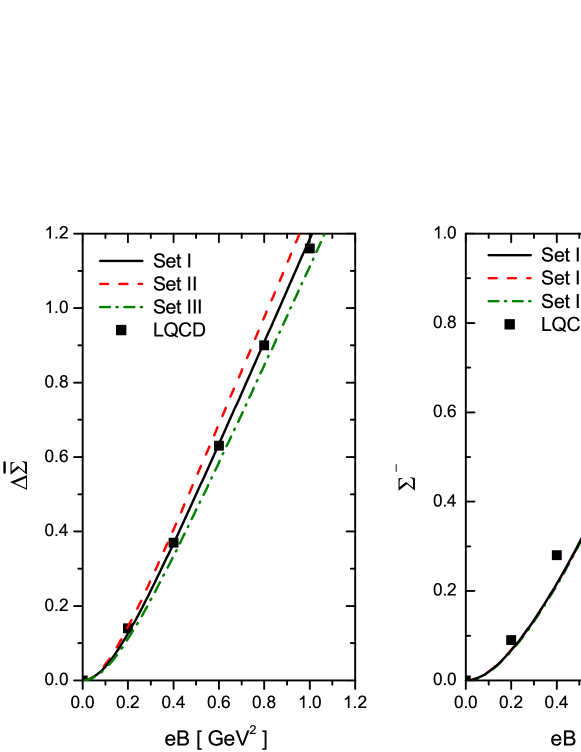
Figure 1: (Color online) Left and right panels show the behavior of $\Delta\bar{\Sigma}$ and $\Sigma^{-}$, respectively, as functions of $eB$ for three different model parameter sets. Results from lattice QCD calculations Bali:2012zg are included for comparison.

In Fig. 2 we show our numerical results for the behavior of pion masses, which are plotted as functions of $eB$. Solid, dashed and dashed-dotted lines correspond to Sets I, II and III, respectively. In the case of the $\pi^{+}$, the curves correspond to the “magnetic-field dependent mass” $E_{\pi^{+}}$ defined by Eq. (41). For comparison we also show the behavior of $E_{\pi^{+}}$ in the case of a point-like meson. From the figure it is seen that, according to the prediction of the model, the $\pi^{+}$ structure tends to increasingly enhance the value of $E_{\pi^{+}}$ when the magnetic field is increased. The figure also includes the LQCD results given in Ref. Bali:2011qj , in which values up to $eB\sim 0.4$ GeV² have been quoted for realistic pion masses using staggered quarks. It is found that model predictions are in good agreement with LQCD results for $eB\lesssim 0.15$ GeV², while they seem to deviate from them for larger values of the magnetic field. Concerning the $\pi^{0}$ mass, it is seen that it shows a slight decrease with $eB$, as previously found e.g. in Refs. Avancini:2015ady ; Avancini:2016fgq . Once again the results are in general rather independent of the model parametrization.

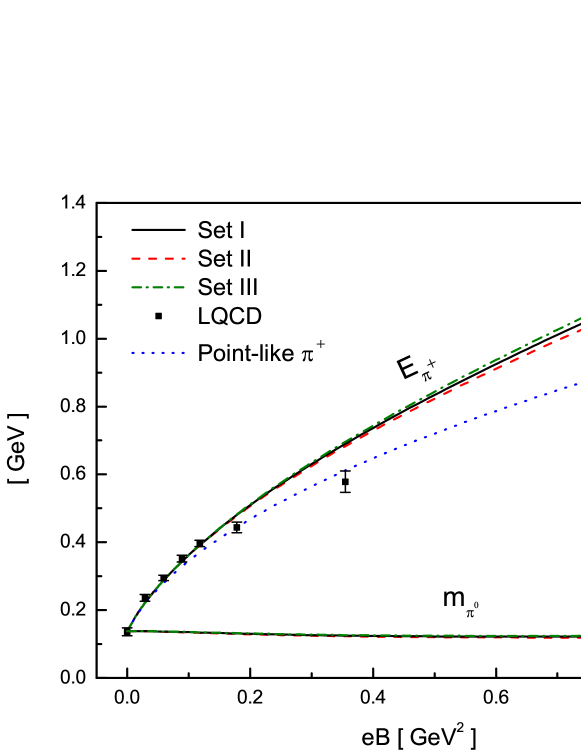
Figure 2: (Color online) Neutral pion mass and magnetic field-dependent charged pion mass as functions of $eB$ for three different model parameter sets (notice that they are practically indistinguishable from each other in the case of the neutral pion). For comparison, the behavior of the magnetic field-dependent mass of a point-like charged pion (dotted line), as well as results from lattice QCD calculations in Ref. Bali:2011qj (squares) are also included.

Besides the mentioned LQCD calculation in Ref. Bali:2011qj , more recent lattice simulations using Wilson fermions Bali:2017ian ; Bali:2017yku have been carried out, providing results for $\pi^{+}$ and $\pi^{0}$ masses for larger values of $eB$. In these simulations, however, a heavy pion with $m_{\pi}(0)=415$ MeV in vacuum has been considered. In order to compare these results with our predictions we follow the procedure done in Ref. Avancini:2016fgq , viz. we consider a parameter Set Ib in which $G$ and $\Lambda$ are the same as in Set I, while $m_{0}$ is increased so as to obtain $m_{\pi}(0)=415$ MeV. Moreover, in Ref. Avancini:2016fgq , the authors also consider a magnetic field dependent coupling $G(eB)$ of the form

$$G(eB)=\alpha+\beta\,e^{-\gamma\,(eB)^{2}}\ ,$$ (44)

in order to reproduce LQCD results for the behavior of quark condensates as well as that of the $\pi^{0}$ mass.

The curves for the normalized charged pion $B$-dependent mass $E_{\pi^{+}}/m_{\pi}(0)$ and neutral pion mass $m_{\pi^{0}}/m_{\pi}(0)$ for Set Ib are shown in Fig. 3 (solid lines), together with LQCD results obtained for these quantities after an extrapolation of lattice spacing to the continuum Bali:2017ian . In addition, we have included in this figure the results corresponding to the parameter Set IV of Ref. Avancini:2016fgq , with the $B$-dependent coupling $G(eB)$. It is seen that for the $\pi^{+}$ meson the results from Set Ib are consistent with lattice data, although the errors in the latter are considerably large to be conclusive (in fact, results obtained considering finite lattice spacings become closer to those corresponding to a point-like $\pi^{+}$ Bali:2017yku ). On the other hand, in the case of the $\pi^{0}$ mass, where errors from LQCD are smaller, the curve obtained from Set Ib appears to be clearly above lattice predictions. Regarding the model proposed in Ref. Avancini:2016fgq , it is seen that the behavior of the $B$-dependent mass of the $\pi^{+}$ is similar to that of a point-like particle, while (as discussed in Ref. Avancini:2016fgq ) the results for the $\pi^{0}$ mass are in good agreement with LQCD data. In the case of that model, it is worth noticing that once $m_{0}$ is rescaled to get a phenomenologically acceptable value for the pion mass, the corresponding parametrization leads to a too low value for the pion decay constant at $B=0$, namely $f_{\pi}\simeq 80$ MeV.

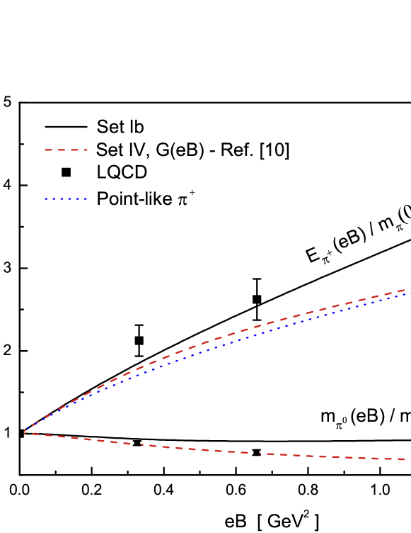
Figure 3: (Color online) Normalized neutral pion mass and magnetic field-dependent charged pion mass as functions of $eB$. Solid lines correspond to the results from Set Ib, while dashed lines are obtained from Set IV of Ref. Avancini:2016fgq , considering a magnetic field-dependent coupling $G(eB)$ as in Eq. (44). The dotted line shows the behavior of the normalized magnetic field-dependent mass of a point-like charged pion, while squares correspond to the results of lattice QCD simulations in Ref. Bali:2017ian , which consider a $B=0$ pion mass of 415 MeV.

In conclusion, we have analyzed the effect of an intense external magnetic field $\vec{B}$ on $\pi$ meson masses within the two-flavor NJL model. In particular, we have shown that the Ritus eigenfunction method allows us to fully take into account the translational-breaking effects introduced into the calculation of the charged meson masses by the Schwinger phases in the RPA approach. For the definition of the magnetic-field dependent mass it has been taken into account that, owing to zero-point motion in the plane perpendicular to $\vec{B}$, the charged pion cannot be at rest in the presence of the magnetic field, even at the lowest Landau level.

In our numerical calculations we have used a model parametrization that satisfactorily describes not only meson properties in the absence of the magnetic field but also the behavior of quark condensates as functions of $B$ obtained in LQCD calculations. We have found that when the magnetic field is enhanced, the $\pi^{0}$ mass shows a slight decrease, while the magnetic-field dependent mass of the charged pion steadily increases, remaining always larger than that of a point-like pion. These results are in agreement with LQCD calculations with realistic pion masses for low values of $eB$ (say $eB\lesssim 0.15$ GeV²), although there seems to be some discrepancy as the magnetic field is increased. For larger values of $eB$, some recent LQCD simulations for $m_{\pi^{0}}$ and $E_{\pi^{+}}$ have been carried out considering unphysically large quark masses. In the case of $E_{\pi^{+}}$ the results are consistent with our calculations (with adequately rescaled parameters), while there is a significant discrepancy in the case of the $\pi^{0}$ mass. On the other hand, it is seen that the agreement for $m_{\pi^{0}}$ gets improved if, as done in Ref. Avancini:2016fgq , a magnetic dependent coupling constant $G(eB)$ is introduced. In this sense, we notice that nonlocal NJL-like models, which naturally predict a magnetic field dependence of the quark current-current interaction, have been shown to adequately reproduce the $\pi^{0}$ mass behavior GomezDumm:2017jij . A proper analysis of the $\pi^{+}$ mass in this framework would be welcome. Concerning the future outlook on this subject, it is clear that within the NJL model the method used in this work will allow for a consistent determination of the charged pion decay constants and the behavior of finite temperature pion properties in the presence of intense magnetic fields. We expect to report on these topics in forthcoming publications.

NNS is grateful to S. Avancini for useful correspondence. This work has been supported in part by CONICET and ANPCyT (Argentina), under grants PIP14-578, PIP12-449, and PICT14-03-0492, and by the National University of La Plata (Argentina), Project No. X718.

References

• (1) D. E. Kharzeev, K. Landsteiner, A. Schmitt and H. U. Yee, Lect. Notes Phys.  871 (2013) 1.
• (2) J. O. Andersen, W. R. Naylor and A. Tranberg, Rev. Mod. Phys.  88 (2016) 025001.
• (3) V. A. Miransky and I. A. Shovkovy, Phys. Rept.  576 (2015) 1.
• (4) D. E. Kharzeev, L. D. McLerran and H. J. Warringa, Nucl. Phys. A 803 (2008) 227; V. Skokov, A. Y. Illarionov, and V. Toneev, Int. J. Mod. Phys. A 24 (2009) 5925; V. Voronyuk, V. Toneev, W. Cassing, E. Bratkovskaya, V. Konchakovski, and S. Voloshin, Phys. Rev. C 83 (2011) 054911.
• (5) R. C. Duncan and C. Thompson, Astrophys. J. 392 (1992) L9; C. Kouveliotou et al., Nature 393 (1998) 235.
• (6) S. Fayazbakhsh, S. Sadeghian and N. Sadooghi, Phys. Rev. D 86 (2012) 085042.
• (7) S. Fayazbakhsh and N. Sadooghi, Phys. Rev. D 88 (2013) 065030.
• (8) S. S. Avancini, W. R. Tavares and M. B. Pinto, Phys. Rev. D 93 (2016) 014010.
• (9) R. Zhang, W. j. Fu and Y. x. Liu, Eur. Phys. J. C 76 (2016) 307.
• (10) S. S. Avancini, R. L. S. Farias, M. Benghi Pinto, W. R. Tavares and V. S. Tim teo, Phys. Lett. B 767 (2017) 247.
• (11) S. Mao and Y. Wang, Phys. Rev. D 96 (2017) 034004.
• (12) D. Gomez Dumm, M. F. I. Villafañe and N. N. Scoccola, Phys. Rev. D, in press, arXiv:1710.08950 [hep-ph].
• (13) Z. Wang and P. Zhuang, arXiv:1712.00554 [hep-ph].
• (14) H. Liu, X. Wang, L. Yu and M. Huang, arXiv:1801.02174 [hep-ph].
• (15) J. O. Andersen, JHEP 1210 (2012) 005.
• (16) N. O. Agasian and I. A. Shushpanov, JHEP 0110 (2001) 006.
• (17) V. D. Orlovsky and Y. A. Simonov, JHEP 1309 (2013) 136.
• (18) M. A. Andreichikov, B. O. Kerbikov, E. V. Luschevskaya, Y. A. Simonov and O. E. Solovjeva, JHEP 1705 (2017) 007.
• (19) G. S. Bali, F. Bruckmann, G. Endrodi, Z. Fodor, S. D. Katz, S. Krieg, A. Schafer and K. K. Szabo, JHEP 1202 (2012) 044.
• (20) Y. Hidaka and A. Yamamoto, Phys. Rev. D 87 (2013) 094502.
• (21) E. V. Luschevskaya, O. E. Solovjeva, O. A. Kochetkov and O. V. Teryaev, Nucl. Phys. B 898 (2015) 627.
• (22) B. B. Brandt, G. Bali, G. Endrodi and B. Glaessle, PoS LATTICE 2015 (2016) 265.
• (23) G. S. Bali, B. B. Brandt, G. Endrodi and B. Glaessle, Phys. Rev. D 97 (2018) 034505.
• (24) G. S. Bali, B. B. Brandt, G. Endrodi and B. Glaessle, arXiv:1710.01502 [hep-lat].
• (25) U. Vogl and W. Weise, Prog. Part. Nucl. Phys.  27 (1991) 195.
• (26) S. P. Klevansky, Rev. Mod. Phys.  64 (1992) 649.
• (27) T. Hatsuda and T. Kunihiro, Phys. Rep.  247 (1994) 221.
• (28) J. S. Schwinger, Phys. Rev.  82 (1951) 664.
• (29) V. I. Ritus, Sov. Phys. JETP 48 (1978) 788.
• (30) S. P. Klevansky and R. H. Lemmer, Phys. Rev. D 39 (1989) 3478.
• (31) D. P. Menezes, M. Benghi Pinto, S. S. Avancini, A. Perez Martinez and C. Providencia, Phys. Rev. C 79 (2009) 035807.
• (32) P. G. Allen, A. G. Grunfeld and N. N. Scoccola, Phys. Rev. D 92 (2015) 074041.
• (33) S. P. Klevansky, J. Janicke and R. H. Lemmer, Phys. Rev. D 43 (1991) 3040.
• (34) G. S. Bali, F. Bruckmann, G. Endrodi, Z. Fodor, S. D. Katz and A. Schafer, Phys. Rev. D 86 (2012) 071502.