Joint Antenna Selection and Phase-only Beamforming using Mixed-Integer Nonlinear Programming

Abstract

In this paper, we consider the problem of joint antenna selection and analog beamformer design in downlink single-group multicast networks. Our objective is to reduce the hardware costs by minimizing the number of required phase shifters at the transmitter while fulfilling given distortion limits at the receivers. We formulate the problem as an $\ell_{0}$ minimization problem and devise a novel branch-and-cut based algorithm to solve the resulting mixed-integer nonlinear program to optimality. We also propose a suboptimal heuristic algorithm to solve the above problem approximately with a low computational complexity. Computational results illustrate that the solutions produced by the proposed heuristic algorithm are optimal in most cases. The results also indicate that the performance of the optimal methods can be significantly improved by initializing with the result of the suboptimal method.

Index Terms—  Sparse optimization, $\ell_{0}$ minimization, antenna selection, low-cost wireless network, massive MIMO, sparse democratic representation.

1 Introduction

Optimal antenna selection under various side constraints is a long-standing open research problem that is fundamental in a number of array processing applications [1, 2, 3]. A traditional approach in optimizing the array geometry, commonly referred to as “array thinning”, consists of eliminating sensors from a large uniform linear array structure with the objective to create a high resolution array with a reduced number of elements [4, 5, 6]. Similarly, in upcoming Massive MIMO systems, dedicated radio frequency (RF) chains for each antenna element are no longer affordable [7, 8]. In order to reduce hardware costs, fast switching networks may be used to adaptively select only a subset of inexpensive MIMO antennas to be connected to a reduced number of costly RF transceiver chains. Similarly, in hybrid beamforming networks based on a bank of fixed analog beamformers (ABFs) [9, 10, 11, 12], generally a large number of ABF outputs is available from which only a small subset can be sampled in the baseband, hence antenna selection in the beamspace domain is the underlying problem. A major challenge in designing analog beamforming solutions for phased arrays stems from the restriction that analog phase shifters only permit phase but no magnitude variations of the antenna signals. Similarly, in digital beamforming using cheap power amplifiers with nonlinear output characteristics, low peak-to-average power ratio (PAPR) outputs are required to avoid signal distortions [13, 14].

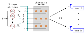
Fig. 1: Schematic diagram of system model.

In this paper, we consider a joint antenna selection and optimal phase-only (constant-modulus) beamforming that can be used for array designs based on the thinning approach as well as antenna and beam selection in hybrid Massive MIMO systems. In our approach we minimize the number of required RF phase shifters by jointly designing the optimal phase values and assigning appropriate antenna elements to the phase shifters, while controlling the resulting beampattern of the thinned array. This problem is cast as an $\ell_{0}$ minimization task for which we devise an efficient algorithm to solve it to (global) optimality and demonstrate its effectiveness in numerical experiments. Our approach allows for an exact solution of the underlying $\ell_{0}$ minimization problem. We also develop a heuristic method that computes high-quality solutions with substantially lower computational effort. The computational results show that the solutions generated by the proposed heuristic method are optimal in most cases, and that the heuristic method can assist in significantly speeding up the optimal methods by providing a better initialization.

2 System Model

We consider a sensor array composed of $N$ antenna elements and a switching network that selects a subset of $M$ antennas to be connected to $M$ phase shifters, where $M\ll N$, as shown in Fig. 1. Let $\mathbf{a}=[a_{1},a_{2},\ldots,a_{M}]^{\mathsf{T}}$ denote the ABF, where the element $a_{m}\in\mathbb{C}$ is the value of the $m$th phase shifter, for $m\in[M]\triangleq\{1,2,\ldots,M\}$. The ABF elements are assumed to be constant modulus, i.e., $\lvert{a_{m}}\rvert=c$ for $m\in[M]$, where $c\in\mathbb{R}$ is a given constant. Let $\mathbf{x}\in\mathbb{C}^{N}$ be the transmit signal vector at the output of the antenna array, where its $n$th element $x_{n}=a_{m}$ if the $n$th antenna element is connected to the $m$th phase shifter and $x_{n}=0$ if the $n$th element is not connected to any phase shifter. There are $K$ single antenna users in the system. We assume without loss of generality (w.l.o.g.) frequency flat channels. Let $\mathbf{h}_{k}\in\mathbb{C}^{N}$ denote the channel vector between the sensor array and the $k$th user, for $k\in[K]\triangleq\{1,2,\ldots,K\}$. We define the channel matrix $\mathbf{H}=[\mathbf{h}_{1},\mathbf{h}_{2},\ldots,\mathbf{h}_{K}]$. Let $\mathbf{s}=[s_{1},s_{2},\ldots,s_{K}]^{\mathsf{T}}$ be the general form of the desired receive signal vector at the user terminals, where the element $s_{k}\in\mathbb{C}$ denotes the desired beamformer output value at the $k$th user. As a special case, in a single-group multicast network, the desired symbol at each user is the same, i.e., $s_{1}=s_{2}=\ldots,s_{K}=s$ and hence $\mathbf{s}=s\mathbf{1}$. In this case, the analog beamformer can be kept constant over the coherence time of the channel, and transmit symbols can be tuned in the digital domain and be transmitted with the help of the phase shifters to serve different symbols in different time slots.

The received signal vector at the users, denoted by $\hat{\mathbf{s}}=[\hat{s}_{1},\hat{s}_{2},\ldots,\hat{s}_{K}]^{\mathsf{T}}$, can be expressed as

$$\hat{\mathbf{s}}=\mathbf{H}^{\mathsf{T}}\mathbf{x}+\mathbf{n},$$ (1)

where $\mathbf{n}\in\mathcal{CN}(\mathbf{0},\sigma^{2}\mathbf{I})$ represents the i.i.d. complex additive white Gaussian noise (AWGN) at the user terminals.

3 Problem Description

In this section, we formulate the problem to optimally design the ABF $\mathbf{a}$ and assign antenna elements to phase shifters. Our objective is to minimize the number of required active antennas such that the root-mean-square error between the desired receive signal vector $\mathbf{s}$ and the actual beamformer output $\hat{\mathbf{s}}$ is at most $\sqrt{\delta}$. The problem can be mathematically expressed as

$$\underset{\mathbf{x}\in\mathbb{C}^{N}}{\operatorname{min\ }} \left\lVert{\mathbf{x}}\right\rVert_{0}$$ (2a)

$$\operatorname{s.t.\ } \left\lVert{\mathbf{s}-\mathbf{H}^{\mathsf{T}}\mathbf{x}}\right\rVert_{2}\leq\sqrt{\delta},$$ (2b)

$$\,\lvert{x_{n}}\rvert\in\{0,c\},\quad\forall n\in[N],$$ (2c)

where $\lVert{{\bf x}}\rVert_{0}\coloneqq\lvert{\{n\in[N]:x_{n}\neq 0\}}\rvert$ denotes the number of nonzero entries of ${\bf x}$, i.e., the number of active antennas. Throughout the remainder of this paper, we assume w.l.o.g. that $c=1$.

By introducing a vector of auxiliary binary variables ${\bf b}=[b_{1},b_{2},\ldots,b_{N}]^{\mathsf{T}}\in\{0,1\}^{N}$, Problem (2) can be reformulated equivalently with a linear objective function as

$$\underset{{\bf x}\in\mathbb{C}^{N},{\bf b}}{\min} \ \sum_{n=1}^{N}b_{n}$$ (3a)

s.t. $$\lVert{\mathbf{s}-\mathbf{H}^{\mathsf{T}}\mathbf{x}}\rVert_{2}\leq\sqrt{\delta},$$ (3b)

$$\lvert{x_{n}}\rvert^{2}=b_{n}, \forall\,n\in[N],$$ (3c)

$$b_{n}\in\{0,1\}, \forall\,n\in[N].$$ (3d)

Let $w_{n}\coloneqq\operatornamewithlimits{Re}[x_{n}]$ and $z_{n}\coloneqq\operatornamewithlimits{Im}[x_{n}]$ denote the real and imaginary part of $x_{n}$, respectively, and let $\mathbf{w}=[w_{1},w_{2},\ldots,w_{N}]^{\mathsf{T}}$ and $\mathbf{z}=[z_{1},z_{2},\ldots,z_{N}]^{\mathsf{T}}$. Then Problem (3) can be written equivalently with real-valued variables as

$$\underset{{\bf w},{\bf z}\in\mathds{R}^{N},{\bf b}}{\min}\ \sum_{n=1}^{N}b_{n}$$ (4a)

s.t. $$\sum_{k=1}^{K}\Big{(}\operatornamewithlimits{Re}[s_{k}]-\left(\operatornamewithlimits{Re}[\mathbf{h}_{k}]^{\mathsf{T}}\mathbf{w}-\operatornamewithlimits{Im}[\mathbf{h}_{k}]^{\mathsf{T}}\mathbf{z}\right)\Big{)}^{2}$$

$$+\Big{(}\operatornamewithlimits{Im}[s_{k}]-\left(\operatornamewithlimits{Re}[\mathbf{h}_{k}]^{\mathsf{T}}\mathbf{z}+\operatornamewithlimits{Im}[\mathbf{h}_{k}]^{\mathsf{T}}\mathbf{w}\right)\Big{)}^{2}\leq{\delta},\quad$$ (4b)

$$w_{n}^{2}+z_{n}^{2}\leq b_{n},\quad\forall\,n\in[N],$$ (4c)

$$w_{n}^{2}+z_{n}^{2}\geq b_{n},\quad\forall\,n\in[N],$$ (4d)

$$b_{n}\in\{0,1\},\,\qquad\forall\,n\in[N].$$ (4e)

Note that we split the modulus constraints $\lvert{x_{n}}\rvert^{2}=w_{n}^{2}+z_{n}^{2}=b_{n}$, $n\in[N]$, into the two inequalities (4c) and (4d) since they will be handled with different techniques.

4 Proposed Algorithm

Problem (4) is a (nonconvex) mixed-integer nonlinear program (MINLP) involving integral variables that are, in fact, binary. Moreover, it contains the convex nonlinear (quadratic) constraints (4b) and (4c), which can be rewritten as second order cone (SOC) constraints. The nonconvexity arises due to the quadratic constraints (4d).

MINLPs can be solved by the so-called spatial branching method, see, for example, [15] for a description. This method employs a general branch-and-bound approach, which branches on integral and continuous variables. In each node of the branch-and-bound tree, a relaxation is solved, which might be strengthened using gradient cuts for convex constraints. For an integral (binary) variable with a fractional solution value, one generates two branches in which the variable is fixed to 0 and 1, respectively. In order to guarantee satisfaction of a possibly violated nonlinear constraint, one also creates branches on a continuous variable by subdividing its feasible region into two parts. The reduced regions allow to strengthen further variable bounds via so-called domain propagation. This in turn allows to strengthen the relaxation. Under appropriate assumptions, the method is guaranteed to converge to a global optimum and terminates in finite time if one considers so-called $\varepsilon$-$\delta$-feasibility, see, e.g., [16].

The general procedure can be enhanced by exploiting particular problem structure. In the following, we show how this can be done for Problem (4). We describe a customized method to propagate domains and to branch on continuous variables using modulus constraints. Moreover, in Section 5, we describe a greedy heuristic method to produce upper bounds for Problem (4). Such bounds allow to prune nodes in the search tree if the value of the relaxation exceeds the upper bound. Implementations of these methods can be incorporated into an MINLP software framework like the non-commercial solver SCIP [17, 18], which makes it easy to employ the general spatial branching method and add the particular customization.

4.1 General Algorithmic Description

In the following, we describe how to solve Problem (4) to global optimality using a branch-and-bound approach that is adapted to the special problem structure.

In each node of the branch-and-bound tree, a linear programming (LP) relaxation of Problem (4) is solved, in which $b_{n}\in\{0,1\}$ is relaxed to $0\leq b_{n}\leq 1$, $n\in[N]$, and constraints (4b), (4c) and (4d) are omitted. In order to strengthen this linear relaxation, we add the following linear inequalities:

$$-b_{n}\leq w_{n} \leq b_{n}, -b_{n}\leq z_{n} \leq b_{n},$$ (5)

$$w_{n}+z_{n} \leq\sqrt{2}\,b_{n}, w_{n}-z_{n} \leq\sqrt{2}\,b_{n},$$

$$-w_{n}+z_{n} \leq\sqrt{2}\,b_{n}, -w_{n}-z_{n} \leq\sqrt{2}\,b_{n};$$

see Figure 2 for a visualization.

We use an LP relaxation in each node of the branch-and-bound tree since this allows for fast warm-starting via the dual simplex algorithm, see, e.g., [19]. In general, the solution of the linear relaxation does not satisfy the nonlinear constraints (4b), (4c) and (4d), and the solution values of $b_{n}$ need not be binary. Thus, for each binary variable with fractional solution value in the LP relaxation, two sub-nodes are created, one for each possible value of the binary variable. This yields tighter LP relaxations in both sub-nodes.

As mentioned above, the error bounding constraints (4b) and the inequalities $w_{n}^{2}+z_{n}^{2}\leq b_{n}$ are convex SOC constraints. If the current LP relaxation solution violates an SOC constraint, it can be cut off by a (linear) gradient cut [20], which is then added to the LP relaxation.

The only remaining inequalities that need to be enforced are the nonconvex lower bound constraints $w_{n}^{2}+z_{n}^{2}\geq b_{n}$, for $n\in[N]$, to which we refer as (lower) modulus constraints. These nonconvex constraints are harder to enforce. If the solution of the current LP relaxation does not yet satisfy these constraints, we generate branching nodes, add linear cuts or propagate domains of variables appearing in the violated modulus constraint. These methods are described in the next subsection.

4.2 Handling Modulus Constraints

Fig. 2: Left: Linear inequalities for strengthening the relaxation. Right: Modulus constraint subdivision into orthants.

If the solution $(\hat{{\bf w}},\hat{{\bf z}},\hat{{\bf b}})$ of the LP relaxation of Problem (4) violates $w_{n}^{2}+z_{n}^{2}\geq b_{n}$ for some $n\in[N]$, we resolve this violation by one of the following steps:

1. If the binary variable $\hat{b}_{n}$ is already fixed to zero, the inequality $w_{n}^{2}+z_{n}^{2}\leq b_{n}$ implies that we can set $\hat{w}_{n},\hat{z}_{n}$ to zero as well.

2. If the bounds of the continuous variables $w_{n}$ and $z_{n}$ are not yet restricted to one of the orthants w.r.t. $w_{n}\times z_{n}$, we create four branching nodes, the first with the additional constraints $w_{n}\geq 0$, $z_{n}\geq 0$, the second with $w_{n}\geq 0$, $z_{n}\leq 0$, the third with $w_{n}\leq 0$, $z_{n}\leq 0$, and the fourth with $w_{n}\leq 0$, $z_{n}\geq 0$. This subdivides the feasible solution set into these four orthants (see Figure 2).

3. If the bounds of the continuous variables $w_{n}$ and $z_{n}$ are already restricted to one of these four orthants, we proceed as described in the following, where we assume w.l.o.g. that $(\hat{w}_{n},\hat{z}_{n},\hat{b}_{n})$ is feasible for the first orthant, i.e., the one with $w_{n}\geq 0$ and $z_{n}\geq 0$.

   • Propagation: Let $l_{1}\leq w_{n}\leq u_{1}$, $l_{2}\leq z_{n}\leq u_{2}$ denote the current lower and upper bounds of the variables $w_{n}$ and $z_{n}$, respectively. Compute the four points $(l_{1},f(l_{1}))$, $(u_{1},f(u_{1}))$, $(f(l_{2}),l_{2})$ and $(f(u_{2}),u_{2})$ on the unit circle that correspond to the respective lower and upper bounds of $w_{n}$ and $z_{n}$, where $f(x)=\sqrt{1-x^{2}}$. These four points can now be used to strengthen the lower and upper bounds of $w_{n}$ and $z_{n}$. In order for an optimal solution $({\bf w}^{\star},{\bf z}^{\star},{\bf b}^{\star})$ to fulfill the modulus constraint $w_{n}^{2}+z_{n}^{2}\geq b_{n}$, the point $(w_{n}^{\star},z_{n}^{\star})$ needs to lie on or above the arc between the two points ($l_{1}^{\prime},u_{2}^{\prime})$ and $(u_{1}^{\prime},l_{2}^{\prime})$ if $b_{n}^{\star}=1$, where

     $$l_{1}^{\prime}=\max\{l_{1},f(u_{2})\},\quad u_{1}^{\prime}=\min\{u_{1},f(l_{2})\},$$

     $$l_{2}^{\prime}=\max\{l_{2},f(u_{1})\},\quad u_{2}^{\prime}=\min\{u_{2},f(l_{1})\}.$$

     This implies that the four values $l_{1}^{\prime}$, $u_{1}^{\prime}$, $l_{2}^{\prime}$ and $u_{2}^{\prime}$ can now be taken as new and possibly strengthened lower and upper bounds of $w_{n}$ and $z_{n}$, respectively. If the binary variable $b_{n}$ is not yet fixed to one, the lower bounds are not propagated, as $b_{n}$ could be set to zero in an optimal solution, implying $w_{n}=z_{n}=0$ as well. A visualization of this propagation is given in Figure 3.

   • Separation: If $\hat{w}_{n}+\hat{z}_{n}<\hat{b}_{n}$, add the cut $w_{n}+z_{n}\geq b_{n}$ to the LP relaxation. Note that each solution in this orthant on the unit circle satisfies this inequality.

   • Branching: If $\hat{w}_{n}+\hat{z}_{n}\geq\hat{b}_{n}$, create two branching nodes defined by inequalities $f_{n}\,w_{n}+g_{n}\,z_{n}\geq b_{n}$, where $f_{n}\in\mathds{R}$ and $g_{n}\in\mathds{R}$ can be computed according to Figure 4.

Fig. 3: Bound propagation for the continuous variables appearing in modulus constraints.

Fig. 4: Inequalities that are added to the sub-nodes.

We prioritize the enforcement of binary variables and SOC constraints over modulus constraints. This means that we do not use the above methods on all modulus constraints, but only “on demand” in case all the other constraints are satisfied and one particular modulus constraint is still violated.

To select a modulus constraint for enforcing, we use a “most infeasible” rule: The idea is to enforce a modulus constraint $w_{\bar{n}}^{2}+z_{\bar{n}}^{2}\geq b_{\bar{n}}$, $\bar{n}\in[N]$, with largest violation. As a measure for the violation of a modulus constraint, we use

$$\rho(n)=\hat{b}_{n}-(\hat{w}_{n}^{2}+\hat{z}_{n}^{2}),$$

i.e., we choose $\bar{n}\in[N]$ with maximal $\rho(\bar{n})$.

The whole solving procedure is summarized in Algorithm 1. Note that it is complete in the following sense: The process will terminate with a point $(\hat{{\bf w}},\hat{{\bf z}},\hat{{\bf b}})$ such that $\hat{w}_{n}=\hat{z}_{n}=0=\hat{b}_{n}$ or $1-\varepsilon\leq\hat{w}_{n}^{2}+\hat{z}_{n}^{2}\leq 1$ and $\hat{b}_{n}=1$.

Input: Node of the branch-and-bound tree with current LP relaxation of the problem including all previously generated cuts, propagated domains and previously computed bounds on the objective value

1 obtain solution $(\hat{{\bf w}},\hat{{\bf z}},\hat{{\bf b}})$ of LP relaxation;

2 if $\hat{{\bf b}}$ is not integral then

3     branch on a fractional binary variable and continue with another node;

4      else if root-mean error constraint (4b) is violated or $\hat{w}_{n}^{2}+\hat{z}_{n}^{2}>\hat{b}_{n}$ for some $n$ then

5          call quadratic constraint handler and possibly continue with another node;

6           else if $\hat{w}_{n}^{2}+\hat{z}_{n}^{2}<\hat{b}_{n}$ then

7               call modulus constraint handler to propagate bounds or branch according to Section 4.2 and continue with another node;

8                else

9                    $(\hat{{\bf w}},\hat{{\bf z}},\hat{{\bf b}})$ is optimal for the current node;

10                     end if

Algorithm 1 Node Solving Procedure within the Branch-and-Bound tree

5 Heuristic Method

Inspired by [21] and [22], we propose a low-complexity suboptimal heuristic method for Problem (2) in the following. Let ${\bf h}^{n}$ represent the channel between the $n$th antenna element at the transmitter to all $K$ users (i.e., the $n$th row of the channel matrix ${\bf H}$), and let $y_{n}$ denote the $n$th element of vector ${\bf y}$. The proposed heuristic is given in Algorithm 2.

We start the suboptimal algorithm with $M=1$ active antenna elements and increase the number of active antenna elements by one in every iteration (in the outermost loop) until we achieve the desired root-mean-square error bound $\sqrt{\delta}$. For each value of $M$, we compute a large number of (max_Iter) suboptimal solutions ${\bf g}_{i}$, each of them resulting from a different random initialization of ${\bf x}$. Note that each of the max_Iter suboptimal solutions ${\bf g}_{i}$ can be computed in parallel to speed up the algorithm.

As illustrated in Algorithm 2, ${\bf x}$ is updated in every iteration (in the innermost loop) such that the root-mean-square error $e$ between the desired and the received signal vector is decreasing. If the smallest error $E_{i^{\star}}$ among all max_Iter errors is smaller than $\sqrt{\delta}$, then the corresponding solution ${\bf g}_{i^{\star}}$ is adopted as the solution of the heuristic method.

Input: ${\bf H}$, ${\bf s}$, $\delta$

1 Initialize $M\leftarrow 1\ (\text{or\ }M^{\text{guess}})$;

2 repeat

3      for i = $1$ to max_Iter do

4           Randomly initialize ${\bf x}\in\mathbb{C}^{N}$ such that $\lVert{{\bf x}}\rVert_{0}=M$ and $\lvert{x_{n}}\rvert\in\{0,1\}$, $n\in[N]$;

5           Compute error $e=\lVert{{\bf s}-{\bf H}^{\mathsf{T}}{\bf x}}\rVert_{2}$;

6           for count = $1$ to max_Count do

7                Assign ${\bf y}\leftarrow{\bf x}$;

8                Randomly select two integers $u$ and $v$ such that $u,v\in[N]$, $\lvert{y_{u}}\rvert=1$ and $y_{v}=0$;

9                Compute the residual ${\bf r}={\bf s}-{\bf H}^{\mathsf{T}}{\bf y}+y_{u}({\bf h}^{u})^{\mathsf{T}}$;

10                $[{y}_{u}^{\star},{y}_{v}^{\star}]=\underset{\bar{y}_{u},\bar{y}_{v}}{\operatorname{argmin\ }}\left\lVert{{\bf r}-\bar{y}_{u}({\bf h}^{u})^{\mathsf{T}}+\bar{y}_{v}({\bf h}^{v})^{\mathsf{T}}}\right\rVert_{2}$;

11                if $\lvert{{y}_{u}^{\star}}\rvert\geq\lvert{{y}_{v}^{\star}}\rvert$ then

12                     ${y}_{u}\leftarrow\dfrac{{y}_{u}^{\star}}{\lvert{{y}_{u}^{\star}}\rvert}$;

13                    

14                     else

15                         ${y}_{u}\leftarrow 0$ and ${y}_{v}\leftarrow\dfrac{{y}_{v}^{\star}}{\lvert{{y}_{v}^{\star}}\rvert}$;

16                         

17                          end if

18                         Compute $\hat{e}=\lVert{{\bf s}-{\bf H}^{\mathsf{T}}{\bf y}}\rVert_{2}$;

19                          if $\hat{e}<e$  then

20                               Update ${\bf x}\leftarrow{\bf y}$ and $e\leftarrow\hat{e}$;

21                              

22                               end if

23                              

24                               end for

25                              ${\bf g}_{i}\leftarrow{\bf x}$ and error $E_{i}\leftarrow e$;

26                              

27                               end for

28                              Compute $i^{\star}=\operatorname{argmin}_{i}\,E_{i}$;

29                               $E^{\star}\leftarrow E_{i^{\star}}$ and $\tilde{{\bf x}}\leftarrow{\bf g}_{i^{\star}}$;

30                               $M\leftarrow M+1$;

31                              

32                               until $E^{\star}\leq\sqrt{\delta}$ or $M>N$;

return $\tilde{{\bf x}}$

Algorithm 2 Suboptimal heuristic algorithm

6 Numerical Experiments

In this section, we evaluate the performance of the proposed modulus handling based optimal method and suboptimal heuristic method in terms of the resulting hardware requirement (number of required phase shifters) and the used computation time. For the computations, we assumed a Rayleigh fading channel. The transmit symbols are obtained by employing quadrature-phase-shift-keying (QPSK) modulation at the transmitter with a constant magnitude $q=1.414$. We used the values $N\in\{16,32,48,64\}$ for the number of antennas, $K\in\{2,3,4\}$ for the number of users and $\delta^{2}\in\{0.1q,0.2q\}$ for the error bounds.

With this setup, we solved Problem (4) with a C implementation using SCIP 4.0.1 [17, 18] and CPLEX 12.7.1 as LP solver on a Linux cluster with 3.5 GHz Intel Xeon E5-1620 Quad-Core CPUs, having 32 GB main memory and 10 MB cache. All computations were performed single-threaded with a time limit of one hour (3600 s). The results are shown in Table Joint Antenna Selection and Phase-only Beamforming using Mixed-Integer Nonlinear Programming.

The table displays the solving time (in seconds) and the number of branch-and-bound nodes for four different algorithm variants. In the first column block, we present the results of the default version of SCIP, which applies no special methods to handle modulus constraints – they are handled like general quadratic constraints. The second block shows the results when the methods for handling modulus constraints as described in Section 4.2 are included in SCIP as a constraint handler. In the third and fourth block, the results of the same two methods as before are presented, but an initial (not necessarily optimal) solution is computed with the suboptimal greedy heuristic method presented in Section 5 and passed to the exact solution method. For the number of iterations of the two inner loops, we chose max_Iter = max_Count = 1000. In all four runs, the reading times of the problem files are included in the solving times, as are the runtimes of the suboptimal heuristic in the third and fourth column block. The last column block shows the sparsity $M$ of the solution computed by the suboptimal heuristic compared to the optimal solution computed by SCIP, as well as the solving time of the suboptimal heuristic.

The bottom part of the table presents geometric, shifted geometric and arithmetic mean of the number of nodes and the solving time. The shifted geometric mean of $t_{1},\dots,t_{n}$ is defined as

$$\bigg{(}\prod_{i=1}^{n}(t_{i}+\Delta)\bigg{)}^{\frac{1}{n}}-\Delta,$$

with the shift factor $\Delta=10$ for times and $\Delta=100$ for nodes. It reduces the influence of easy instances on the mean values.

It turns out that the default version of SCIP already performs quite well. For $K=2$ users, the running times are very fast even for large values of $N$. For $K\in\{3,4\}$ users and a very small error bound $\delta^{2}=0.1q$, the instances are much harder to solve. From the shifted geometric mean in the bottom line, it can be seen that adding the modulus constraint handler to SCIP results in a significantly faster running time (about 26 % faster). However, the number of processed nodes does not significantly change. The shifted geometric mean of the number of nodes that were produced by the modulus constraint handler is 787.25 (about 24 %).

Executing the suboptimal heuristic and passing its solution to SCIP greatly helps in solving the optimization problem on average, even in the default version of SCIP. Also, the number of nodes is reduced significantly, since many nodes of the branch-and-bound tree can be pruned. Note, however, that for the easier problems the suboptimal heuristic consumes almost all of the solving time. Again, adding the modulus constraint handler to SCIP speeds up the solving process (about 15 % and 39 % speed-up compared to the default with and without initial solution, respectively), but the number of nodes does not decrease. The shifted geometric mean of the number of nodes produced by the modulus constraint handler is 255.43. Comparing to the total number of nodes (500) shows that about half of the branching nodes are used to branch on binary variables.

It is worth mentioning that the suboptimal heuristic actually returns the optimal sparsity level in all but four instances. We observe that only for large instances the heuristic is indeed suboptimal, but these instances cannot be solved by SCIP within the time limit, regardless of adding the modulus constraint handler. Interestingly, one of the instances of Table Joint Antenna Selection and Phase-only Beamforming using Mixed-Integer Nonlinear Programming for which the heuristic computes a suboptimal solution runs into the time limit with the default version of SCIP when this solution is passed as starting solution. However, if the suboptimal solution is not computed beforehand, SCIP solves this instance in roughly 700 s. One possible explanation is the so-called performance variability (small changes in the problem or solution process lead to large changes in performance).

7 Conclusion

In this paper, we considered joint antenna selection and design of phase-only analog beamformers. Our goal was to minimize the hardware requirement by reducing the number of phase shifters and active antenna elements required to achieve a given maximum distortion requirement at the receivers. We formulated the problem as an $\ell_{0}$ minimization program and proposed an efficient algorithm to solve it to global optimality. We also presented a low-complexity suboptimal heuristic method to solve the problem approximately. The computational results illustrate the proposed heuristic method yields optimal solutions in most cases, with substantially reduced computational complexity. The results also revealed that, in general, the practical complexity of the optimal methods can be drastically reduced by initializing them with the suboptimal solutions obtained from the proposed heuristic method.

Table 1: Analysis and performance evaluation of different solution approaches/settings (SCIP 4.0.1 in optimized mode, reading time included in solving time).

	default SCIP		modulus handling		default SCIP		modulus handling		suboptimal heuristic
					+ suboptimal heuristic		+ suboptimal heuristic
Instance	#nodes	time (s)	#nodes	time (s)	#nodes	time (s)	#nodes	time (s)	opt. sol.	subopt. sol.	time (s)
$N=16,K=2,\delta^{2}=0.1q$, no=1	469	1.6	501	1.6	7	3.5	9	3.5	2	2	3.29
$N=16,K=2,\delta^{2}=0.1q$, no=2	863	2.1	418	1.1	6	3.5	6	3.4	2	2	3.28
$N=16,K=2,\delta^{2}=0.2q$, no=1	11	0.5	11	0.5	1	3.4	1	3.3	2	2	3.28
$N=16,K=2,\delta^{2}=0.2q$, no=2	190	0.8	136	0.6	1	3.3	1	3.3	2	2	3.29
$N=16,K=3,\delta^{2}=0.1q$, no=1	3 908	9.6	2 044	4.8	998	14.0	1 118	11.4	4	4	9.47
$N=16,K=3,\delta^{2}=0.1q$, no=2	1 690	4.9	2 337	4.6	996	14.0	928	12.1	4	4	9.42
$N=16,K=3,\delta^{2}=0.2q$, no=1	1 704	7.9	1 529	3.5	47	8.8	71	8.7	3	3	7.08
$N=16,K=3,\delta^{2}=0.2q$, no=2	2 688	7.5	1 720	3.3	87	8.4	95	8.3	3	3	7.10
$N=16,K=4,\delta^{2}=0.1q$, no=1	25 507	121.8	22 684	40.7	2 374	27.7	2 470	20.9	5	5	16.39
$N=16,K=4,\delta^{2}=0.1q$, no=2	2 853	10.4	2 603	6.5	95	14.9	133	14.9	4	4	13.04
$N=16,K=4,\delta^{2}=0.2q$, no=1	2 533	11.0	1 481	3.9	289	15.6	393	15.6	4	4	13.06
$N=16,K=4,\delta^{2}=0.2q$, no=2	12 676	57.2	11 591	20.7	13 095	73.6	9 637	28.2	5	5	16.41
$N=32,K=2,\delta^{2}=0.1q$, no=1	170	7.5	204	9.6	4	4.2	4	4.2	2	2	4.04
$N=32,K=2,\delta^{2}=0.1q$, no=2	1 937	6.2	714	2.2	2	4.2	2	4.2	2	2	3.97
$N=32,K=2,\delta^{2}=0.2q$, no=1	201	2.7	203	1.4	6	4.4	8	4.3	2	2	3.98
$N=32,K=2,\delta^{2}=0.2q$, no=2	101	2.8	41	1.6	17	4.5	11	4.4	2	2	3.99
$N=32,K=3,\delta^{2}=0.1q$, no=1	12 910	52.1	5 582	16.5	77	13.5	134	12.9	3	3	8.53
$N=32,K=3,\delta^{2}=0.1q$, no=2	313	1.7	356	1.6	177	13.1	210	14.3	3	3	8.58
$N=32,K=3,\delta^{2}=0.2q$, no=1	3 387	12.0	2 671	9.6	159	13.9	198	13.8	3	3	8.52
$N=32,K=3,\delta^{2}=0.2q$, no=2	1 380	7.2	2 514	10.7	143	14.1	151	14.2	3	3	8.61
$N=32,K=4,\delta^{2}=0.1q$, no=1	96 569	559.3	13 703	51.0	154 122	652.4	57 158	156.6	4	5	19.59
$N=32,K=4,\delta^{2}=0.1q$, no=2	141 531	816.5	97 762	301.4	147 573	648.7	66 224	172.8	5	5	18.29
$N=32,K=4,\delta^{2}=0.2q$, no=1	8 070	31.9	9 874	37.2	43	15.6	42	15.0	3	3	11.75
$N=32,K=4,\delta^{2}=0.2q$, no=2	4 879	20.5	14 224	52.9	97	16.5	123	16.7	3	3	11.73
$N=48,K=2,\delta^{2}=0.1q$, no=1	496	8.7	315	8.2	1	4.9	1	4.9	2	2	4.64
$N=48,K=2,\delta^{2}=0.1q$, no=2	190	2.0	734	5.0	9	5.1	9	5.1	2	2	4.59
$N=48,K=2,\delta^{2}=0.2q$, no=1	15	1.6	447	3.1	7	5.0	7	5.0	2	2	4.58
$N=48,K=2,\delta^{2}=0.2q$, no=2	201	2.9	487	4.5	7	4.9	7	4.9	2	2	4.58
$N=48,K=3,\delta^{2}=0.1q$, no=1	2 256	18.9	8 253	49.2	259	16.3	283	16.4	3	3	9.85
$N=48,K=3,\delta^{2}=0.1q$, no=2	39 191	236.6	5 542	31.4	285	19.7	332	20.0	3	3	9.90
$N=48,K=3,\delta^{2}=0.2q$, no=1	1 810	21.8	2 777	19.5	381	20.5	484	20.8	3	3	9.87
$N=48,K=3,\delta^{2}=0.2q$, no=2	3 648	27.2	2 207	11.2	347	23.1	362	22.9	3	3	9.91
$N=48,K=4,\delta^{2}=0.1q$, no=1	104 244	992.9	56 336	354.9	168 481	2477.0	107 320	439.4	4	5	22.63
$N=48,K=4,\delta^{2}=0.1q$, no=2	70 950	465.3	28 474	177.2	4 895	64.2	6 357	62.8	4	4	17.99
$N=48,K=4,\delta^{2}=0.2q$, no=1	9 764	65.4	29 631	170.3	83	24.2	91	24.6	3	3	13.53
$N=48,K=4,\delta^{2}=0.2q$, no=2	56 580	373.8	67 515	348.5	9 933	86.9	11 707	76.0	4	4	18.09
$N=64,K=2,\delta^{2}=0.1q$, no=1	397	4.2	273	3.3	10	5.7	10	5.7	2	2	5.18
$N=64,K=2,\delta^{2}=0.1q$, no=2	360	4.0	360	3.9	11	5.7	11	5.7	2	2	5.17
$N=64,K=2,\delta^{2}=0.2q$, no=1	505	4.5	931	7.0	8	5.7	8	5.7	2	2	5.19
$N=64,K=2,\delta^{2}=0.2q$, no=2	476	4.8	481	4.8	11	6.0	11	6.0	2	2	5.19
$N=64,K=3,\delta^{2}=0.1q$, no=1	11 498	105.5	5 982	36.5	529	33.0	568	32.6	3	3	11.17
$N=64,K=3,\delta^{2}=0.1q$, no=2	6 464	70.6	20 879	105.7	279	21.9	333	21.9	3	3	11.17
$N=64,K=3,\delta^{2}=0.2q$, no=1	830	12.2	884	11.9	519	34.2	512	34.5	3	3	11.24
$N=64,K=3,\delta^{2}=0.2q$, no=2	6 626	59.2	9 821	57.0	815	34.8	966	34.2	3	3	11.22
$N=64,K=4,\delta^{2}=0.1q$, no=1	217 176	3128.0	360 779	2932.9	20 299	172.6	24 143	152.2	4	4	20.38
$N=64,K=4,\delta^{2}=0.1q$, no=2	75 975	670.0	329 245	2982.6	$>$157 627	$>$3600.0	510 570	3492.6	4	5	25.50
$N=64,K=4,\delta^{2}=0.2q$, no=1	51 999	688.0	47 384	396.5	10 226	126.6	28 560	185.1	3	4	20.58
$N=64,K=4,\delta^{2}=0.2q$, no=2	82 051	748.6	26 076	173.8	119	35.1	123	35.4	3	3	15.24
Geometric mean	2 796	21.6	2 816	16.0	164	19.6	178	17.3
Shifted geometric mean	3 308	36.5	3 228	27.5	470	26.4	500	22.4
Arithmetic mean	22 296	197.3	25 014	176.8	14 490	175.6	17 331	110.0

References

- [1] R. W. Heath, S. Sandhu, and A. Paulraj, “Antenna selection for spatial multiplexing systems with linear receivers,” IEEE Commun. Letters, vol. 5, no. 4, pp. 142–144, Apr. 2001.
- [2] S. Sanayei and A. Nosratinia, “Antenna selection in MIMO systems,” IEEE Commun. Mag., vol. 42, no. 10, pp. 68–73, Oct. 2004.
- [3] D. A. Gore and A. J. Paulraj, “MIMO antenna subset selection with space-time coding,” IEEE Trans. Signal Process., vol. 50, no. 10, pp. 2580–2588, Oct. 2002.
- [4] W. P. M. N. Keizer, “Linear array thinning using iterative FFT techniques,” IEEE Trans. Antennas and Propagation, vol. 56, no. 8, pp. 2757–2760, Aug. 2008.
- [5] G. Oliveri, M. Donelli, and A. Massa, “Linear array thinning exploiting almost difference sets,” IEEE Trans. Antennas and Propagation, vol. 57, no. 12, pp. 3800–3812, Dec. 2009.
- [6] A. Jäger et al., “Air-coupled 40-kHz ultrasonic 2D-phased array based on a 3D-printed waveguide structure,” in 2017 IEEE Int. Ultrasonics Symposium (IUS), Sep. 2017.
- [7] E. G. Larsson, O. Edfors, F. Tufvesson, and T. L. Marzetta, “Massive MIMO for next generation wireless systems,” IEEE Commun. Mag., vol. 52, no. 2, pp. 186–195, Feb. 2014.
- [8] L. Lu et al., “An overview of massive MIMO: Benefits and challenges,” IEEE J. Select. Topics in Signal Process., vol. 8, no. 5, pp. 742–758, Oct. 2014.
- [9] O. E. Ayach et al., “Spatially sparse precoding in millimeter wave MIMO systems,” IEEE Trans. Wireless Commun., vol. 13, no. 3, pp. 1499–1513, Mar. 2014.
- [10] T. E. Bogale and L. B. Le, “Beamforming for multiuser massive MIMO systems: Digital versus hybrid analog-digital,” in Proc. IEEE Global Commun. Conf. (GLOBECOM), Austin, TX, USA, Dec. 2014, pp. 4066–4071.
- [11] G. Hegde, Y. Cheng, and M. Pesavento, “Hybrid beamforming for large-scale MIMO systems using uplink-downlink duality,” in Proc. IEEE Int. Conf. on Acoustics, Speech and Signal Process. (ICASSP), Mar. 2017, pp. 3484–3488.
- [12] W. Roh et al., “Millimeter-wave beamforming as an enabling technology for 5G cellular communications: Theoretical feasibility and prototype results,” IEEE Commun. Mag., vol. 52, no. 2, pp. 106–113, Feb. 2014.
- [13] S. K. Deng and M. C. Lin, “Recursive clipping and filtering with bounded distortion for PAPR reduction,” IEEE Trans. Commun., vol. 55, no. 1, pp. 227–230, Jan. 2007.
- [14] S. Han and J. H. Lee, “PAPR reduction of OFDM signals using a reduced complexity PTS technique,” IEEE Signal Process. Letters, vol. 11, no. 11, pp. 887–890, Nov. 2004.
- [15] S. Vigerske and A. Gleixner, “SCIP: Global optimization of mixed-integer nonlinear programs in a branch-and-cut framework,” Optimization Methods and Software, 2017, to appear.
- [16] R. Horst and H. Tuy, Global Optimization: Deterministic Approaches, Springer, Berlin, 3 edition, 1996.
- [17] SCIP, “Solving Constraint Integer Programs,” http://scip.zib.de.
- [18] S. J. Maher et al., “The SCIP optimization suite 4.0,” Tech. Rep. 17-12, ZIB, Takustr.7, 14195 Berlin, 2017.
- [19] A. Schrijver, Theory of linear and integer programming, John Wiley & Sons, 1998.
- [20] S. Vigerske, Decomposition in multistage stochastic programming and a constraint integer programming approach to mixed-integer nonlinear programming, Ph.D. thesis, Humboldt-Universität zu Berlin, 2013.
- [21] Y. Shechtman, A. Beck, and Y. C. Eldar, “GESPAR: Efficient phase retrieval of sparse signals,” IEEE Transactions on Signal Processing, vol. 62, no. 4, pp. 928–938, Feb 2014.
- [22] Christoph Studer, Tom Goldstein, Wotao Yin, and Richard G. Baraniuk, “Democratic representations,” CoRR abs/1401.3420, 2014.