Invariant surfaces in Euclidean space with a log-linear density

Abstract

A $\lambda$-translating soliton with density vector $\vec{v}$ is a surface in Euclidean space whose mean curvature $H$ satisfies $2H=2\lambda+\langle N,\vec{v}\rangle$, where $N$ is the Gauss map. We classify all $\lambda$-translating solitons that are invariant by a one-parameter group of translations and a one-parameter group of rotations.

Keywords: translating soliton, mean curvature, invariant surface, phase plane
AMS Subject Classification: 53A10, 53C44, 53C21, 53C42

1 Introduction

Fix a unit vector $\vec{v}$ in Euclidean space $\mathbb{R}^{3}$ and $\lambda$ a real number. In this paper we study orientable surfaces $\Sigma$ in $\mathbb{R}^{3}$ whose mean curvature $H$ satisfies

$$H(p)=\lambda+\frac{\langle N(p),\vec{v}\rangle}{2},\quad p\in\Sigma,$$ (1)

where $N$ is the Gauss map of $\Sigma$. The interest of this equation is due to its relation with manifolds with density. Indeed, consider $\mathbb{R}^{3}$ with a positive smooth density function $e^{\phi}$ , $\phi\in C^{\infty}(\mathbb{R}^{3})$, which serves as a weight for the volume and the surface area. The first variation of the area $A_{\phi}$ with density $e^{\phi}$ under compactly supported variations and with variation vector field $\xi$ is

$$\frac{d}{dt}{\Big{|}}_{t=0}A_{\phi}(t)=-2\int_{\Sigma}H_{\phi}\langle N,\xi\rangle dA_{\phi},$$

where $H_{\phi}=H-\frac{1}{2}\frac{d\phi}{dN}$. Then it is immediate that $\Sigma$ is a critical point of $A_{\phi}$ for a given weighted volume if and only if $H_{\phi}$ is a constant function $H_{\phi}=\lambda$: see [5, 12]. In this paper we are interested in the log-linear density $e^{\phi}$ where

$$\phi:\mathbb{R}^{3}\rightarrow\mathbb{R},\quad\phi(q)=\langle q,\vec{v}\rangle,$$

and $\vec{v}$ is a unit fixed vector of $\mathbb{R}^{3}$. Then $H_{\phi}=H-\langle N,\vec{v}\rangle/2$ and $H_{\phi}=\lambda$ is exactly (1).

Definition 1.1.

A surface $\Sigma$ in $\mathbb{R}^{3}$ is called a $\lambda$-translating soliton if Eq. (1) holds everywhere. The vector $\vec{v}$ is called the density vector.

A particular case of (1) is when $\lambda=0$, because the equation $2H=\langle N,\vec{v}\rangle$ appears in the singularity theory of the mean curvature flow, indeed, it is the equation of the limit flow by a proper blow-up procedure near type II singular points ([7, 8, 17]). In the literature, a solution of $H_{\phi}=0$ is called a translating soliton of the mean curvature flow. Equation (1) can viewed as a type of prescribed mean curvature equation, in fact, and in a nonparametric form, the equation $H_{\phi}=0$ appeared in the classical article of Serrin [14, p. 477–478] and it was studied in the context of the maximum principle.

It is immediate that if we reverse the orientation on a $\lambda$-translating soliton, then we obtain a $-\lambda$-translating soliton. It is also clear that every rigid motion of $\mathbb{R}^{3}$ that leaves invariant the term $\langle N(p),\vec{v}\rangle$ in (1) is a transformation that preserves the value of $H_{\phi}$. This occurs when we consider a translation, a rotation about a straight line parallel to $\vec{v}$ or a reflection about a plane parallel to $\vec{v}$.

Some examples of $\lambda$-translating solitons are:

1. The case $\lambda=0$ has been widely studied in the literature. Some explicit examples of translating solitons are: a plane parallel to $\vec{v}$, the grim reaper (a surface of translation type, see Sec. 3) and the bowl soliton (a rotational surface). We refer to the reader the next references without to be a complete list: [1, 2, 6, 10, 11, 15, 16, 17].

2. A plane orthogonal to $\vec{v}$ is a $1/2$-translating soliton.

3. A circular cylinder of radius $r>0$ whose axis is parallel to $\vec{v}$ is a $1/(2r)$-translating soliton.

In this paper we consider $\lambda$-translating solitons that are invariant by a one-parameter group of translations and a one-parameter group of rotations. In the first case, the group is characterized by the translation vector $\vec{a}$ and in the second one, by the rotation axis $\vec{a}$. We point out there is not an a priori relation between the direction $\vec{a}$ and the density vector $\vec{v}$ and a purpose of this paper is to study both types of invariant $\lambda$-translating solitons in all its generality. We now give an approach to both settings.

Invariant surfaces by a one-parameter group of translations are related with the one-dimensional problem of Eq. (1) by considering a planar curve $\gamma:I\rightarrow\mathbb{R}^{2}$, $\gamma=\gamma(s)$, whose curvature $\kappa$ satisfies

$$\kappa(s)=\lambda+\langle{\textbf{n}}(s),\vec{w}\rangle,\qquad s\in I,$$ (2)

where $\vec{w}$ is a fixed vector of $\mathbb{R}^{2}$ and ${\textbf{n}}(s)$ is the principal unit normal vector of $\gamma$. Examples of solutions of (2) are straight lines parallel to $\vec{w}$ ($\lambda=0$) and straight lines orthogonal to $\vec{w}$ ($\lambda=1$). With a solution $\gamma$ of (2), we can construct a $\lambda$-translating soliton in $\mathbb{R}^{3}$ invariant by a group of translations as follows. If $(x,y,z)$ stand for the usual coordinates of $\mathbb{R}^{3}$, we place $\gamma$ in the $yz$-plane and consider the cylindrical surface $\Sigma_{\gamma}=\gamma(I)\times\mathbb{R}e_{1}$, where $e_{1}=(1,0,0)$. Then it is immediate that $\Sigma_{\lambda}$ is a $\lambda/2$-translating soliton with density vector $\vec{v}=(0,\vec{w})$ and $\Sigma_{\lambda}$ is invariant by the group of translations generated by $e_{1}$.

In general, a surface $\Sigma$ invariant by a one-parameter group of translations can be parametrized as $X(s,t)=\alpha(s)+t\vec{a}$, where $\alpha$ is a planar curve and $\vec{a}$ is a unit vector orthogonal to the plane containing $\gamma$ and it is called a cylindrical surface. In the above example $\Sigma_{\gamma}$, the translation vector $\vec{a}$ is orthogonal to the density vector $\vec{v}$. In Sec. 2 we study all $\lambda$-translating solitons that are cylindrical surfaces, obtaining in Th. 2.4 a complete classification of these surfaces. This classification depends on the value of $\lambda$ and the vectors $\vec{a}$ and $\vec{v}$. We point out here that for a certain range of values of $\lambda$, there exist entire convex surfaces. In Sec. 3 we extend the notion of cylindrical surface studying $\lambda$-translating solitons which are the sum of two planar curves of $\mathbb{R}^{3}$ contained in orthogonal planes and we classify these surfaces in Th. 3.1.

In Sec. 4 we study $\lambda$-translating solitons invariant by a one-parameter group of rotations and Ths. 4.8 and 4.9 give a complete classification of the rotational $\lambda$-translating solitons. Firstly, we prove that the rotational axis must parallel to the density vector. Next, we prove in Th. 4.1 that there no exist closed $\lambda$-translating solitons, in particular, there are not closed rotational examples. Among the examples that appear in our classification, we point out that for some range of $\lambda$, there exist embedded surfaces that meet the rotational axis orthogonally which are asymptotic to right circular cylinders. We also find convex entire graphs. Finally, in Sect. 5 we prove that if a $\lambda$-translating soliton is foliated by circles in parallel planes orthogonal to the density vector, then the surface must be a surface of revolution.

2 Cylindrical translating solitons

In this section we study $\lambda$-translating solitons invariant by a one-parameter group of translations $G=\{M_{t}:t\in\mathbb{R}\}$, where $M_{t}$ is the translation $M_{t}(p)=p+t\vec{a}$, $p\in\mathbb{R}^{3}$ and $|\vec{a}|=1$. A surface $\Sigma\subset\mathbb{R}^{3}$ invariant by a such group is said a cylindrical surface. It follows from the definition that a global parametrization of $\Sigma$ is $X(s,t)=\alpha(s)+t\vec{a}$, $s\in I$, $t\in\mathbb{R}$, where $\alpha:I\rightarrow\mathbb{R}^{3}$ is a curve whose trace is contained in a plane orthogonal to $\vec{a}$. The mean curvature of $\Sigma$ is $H(X(s,t))=\kappa(s)/2$, where $\kappa$ is the curvature of $\alpha$. Therefore Eq. (1) is

$$\kappa(s)=2\lambda+\mbox{det}(\alpha^{\prime}(s),\vec{a},\vec{v}).$$ (3)

It is immediate that if $\alpha$ is a straight line with direction $\vec{w}$, then $\alpha$ satisfies (3) with $2\lambda=-\mbox{det}(\vec{w},\vec{a},\vec{v})$. Also, if $\vec{a}$ is parallel to $\vec{v}$, then (3) is equivalent to $\kappa=2\lambda$ is constant and thus, $\alpha$ is a straight line or $\alpha$ is a circle of radius $1/(2\lambda)$. We collect these cases:

Proposition 2.1.

1. A plane is a $\lambda$-translating soliton of cylindrical type for any density vector.

2. Planes and right circular cylinders are the only $\lambda$-translating solitons of cylindrical type whose rulings are parallel to the density vector.

Other particular case is $\lambda=0$, that is, $\Sigma$ is a translating soliton. It is known that when $\vec{a}$ is orthogonal to $\vec{v}$, then the only cylindrical translating soliton is a plane parallel to $\vec{a}$ and the grim reaper [11]. A parametrization of this surface for $\vec{a}=(1,0,0)$ and $\vec{v}=(0,0,1)$ is $X(s,t)=(t,s,-\log|\cos(s)|)$.

We now solve (3) in all its generality. Up to a change of coordinates, we take $\vec{a}=(1,0,0)$ and after a rotation about $\vec{a}$, we suppose $\vec{v}=(v_{1},0,v_{3})$, with $v_{3}\geq 0$, $|\vec{v}|=1$. Then the parametrization of $\Sigma$ is $X(s,t)=(t,y(s),z(s))$, where $s\in I,t\in\mathbb{R}$ and the curve $\alpha(s)=(0,y(s),z(s))$ is assumed to be parametrized by arc-length. Denote $\theta$ the angle that makes the velocity $\alpha^{\prime}(s)$ with the $y$-axis and let $y^{\prime}(s)=\cos\theta(s)$ and $z^{\prime}(s)=\sin\theta(s)$ for a certain function $\theta$. The derivative $\theta^{\prime}(s)$ is just the curvature $\kappa$ of $\alpha$. If $\Sigma$ is oriented with respect to the Gauss map $N(t,s)=(0,\sin\theta(s),-\cos\theta(s))$, then (3) is equivalent to

$$\left\{\begin{array}[]{lll}y^{\prime}(s)&=&\displaystyle\cos\theta(s)\\ z^{\prime}(s)&=&\displaystyle\sin\theta(s)\\ \theta^{\prime}(s)&=&2\lambda+v_{3}\cos\theta(s).\end{array}\right.$$ (4)

After a translation in the $yz$-plane we suppose that the initial conditions are

$$y(0)=0,\ \ z(0)=0,\ \ \theta(0)=\theta_{0},$$ (5)

and denote $\{y(s;\lambda,\theta_{0}),z(s;\lambda,\theta_{0}),\theta(s;\lambda,\theta_{0})\}$ the solution of (4)-(5). It is immediate that the solutions are defined in $\mathbb{R}$ because the derivatives $y^{\prime},z^{\prime}$ and $\theta^{\prime}$ are bounded. By Prop. 2.1, we now assume that the function $\theta$ is not constant and that $v_{3}>0$. The solutions of (4) satisfy the next symmetric properties:

Proposition 2.2.

Let $\alpha(s)=(y(s),z(s))$ be a solution of (4).

1. If the curvature of $\alpha$ vanishes at some point, then $\alpha$ is a straight line.

2. If the tangent vector of $\alpha$ is horizontal at some point $s_{0}$, then the graphic of $\alpha$ is symmetric with respect to the vertical straight line $y=y(s_{0})$.

Proof.

1. Suppose $s=0\in I$ is a point where the curvature of $\alpha$ vanishes, that is, $\theta^{\prime}(0)=0$. Let $\theta_{0}=\theta(0)$. By the third equation in (4), we have $2\lambda=-v_{3}\cos\theta_{0}$. The functions $\{\bar{y},\bar{z},\bar{\theta}\}$ defined as

   $$\bar{y}(s)=(\cos\theta_{0})s+y(0)$$

   $$\bar{z}(s)=(\sin\theta_{0})s+z(0)$$

   $$\bar{\theta}(s)=\theta_{0}$$

   satisfy (4) with the same initial conditions at $s=0$ that $\{y,z,\theta\}$. By uniqueness of ODE, $\{y,z,\theta\}=\{\bar{y},\bar{z},\bar{\theta}\}$, proving the result.

2. After a change in the parameter, suppose $s_{0}=0$. Since $\alpha^{\prime}(0)$ is horizontal, then up to an integer multiply of $2\pi$, we have $\theta(0)=0$ or $\theta(0)=\pi$. Suppose $\theta(0)=0$ (similarly for the other case). Then the functions $\{y,z,\theta\}$ satisfy (4) with initial conditions $(0,0,0)$. Define

   $$\bar{y}(s) = -y(-s)+2y(0)$$

   $$\bar{z}(s) = z(-s)$$

   $$\bar{\theta}(s) = -\theta(-s).$$

   Then it is immediate that $\{\bar{y},\bar{z},\bar{\theta}\}$ satisfy (4) with the same initial conditions at $s=0$, and thus $\{\bar{y}(s),\bar{z}(s)\}=\{y(s),z(s)\}$, proving the result.

∎

We relate the shape of a $\lambda$-translating cylindrical surface when we change the sign of $\lambda$. We point out that the computation of $\lambda$ in (4) was obtained by fixing an orientation on $\Sigma$ and thus we have to consider any value of $\lambda$. In the next result, we prove that the graphics of a solution of (4) for $\lambda$ and $-\lambda$ coincide up to reparametrizations.

Proposition 2.3.

For suitable initial conditions in (5), the graphic of a solution of (4) for $\lambda$ coincides with the graphic of a solution of (4) for $-\lambda$ and we have

$$(y(s;\lambda,\theta_{0}),z(s;\lambda,\theta_{0})\}=\{-y(s;-\lambda,\pi-\theta_{0}),z(s;-\lambda,\pi-\theta_{0})),\ s\in\mathbb{R}.$$

Proof.

The functions

$$\bar{y}(s) = -y(s;-\lambda,\pi-\theta_{0}),$$

$$\bar{z}(s) = z(s;-\lambda,\pi-\theta_{0}),$$

$$\bar{\theta}(s) = \pi-\theta(s;-\lambda,\pi-\theta_{0}),$$

satisfy (4) with $(0,0,\theta_{0})$ as initial conditions at $s=0$, proving the result. ∎

The next result classifies all non-planar $\lambda$-translating solitons that are cylindrical surfaces whose density vector is non-parallel to the rulings.

Theorem 2.4.

Let $\alpha(s)=(y(s;\lambda),z(s;\lambda))$ be a solution of (4)-(5) which is not a straight line. After a change of the initial conditions in (5), and by Prop. 2.3, we assume $\lambda\geq 0$ and $\vec{v}=(v_{1},v_{2},v_{3})$, $v_{3}>0$. Then we have:

1. Case $\lambda>v_{3}/2$. The graphic of $\alpha$ is invariant by a discrete group of horizontal translations in the $yz$-plane and the angle function $\theta$ rotates infinitely times around the origin. See Fig. 1, left.

2. Case $\lambda=v_{3}/2$. The graphic of $\alpha$ has one self-intersection point and it is symmetric about a vertical line. See Fig. 1, right.

3. Case $0<\lambda<v_{3}/2$. The graphic of $\alpha$ has two branches asymptotic to two lines of slopes $\pm\tan\theta_{1}$, where $2\lambda+\cos\theta_{1}=0$. Depending on the initial values, we have:

   1. The curve $\alpha$ is symmetric about a vertical line, it has one point of self intersection. See Fig. 2, left.

   2. The curve $\alpha$ is a convex graph on the $y$-real line. See Fig. 2, middle.

4. Case $\lambda=0$. The solution is the grim reaper. See Fig. 2, right.

Proof.

Since $\alpha$ is not a straight line, Prop. 2.2 asserts that the derivative of $\theta$ cannot vanish, and thus $\theta=\theta(s)$ is a monotone function. The monotonicity of $\theta$ is given by the value $\theta^{\prime}(0)=2\lambda+v_{3}\cos\theta_{0}$.

1. Case $\lambda>v_{3}/2$. Then $\theta^{\prime}=2\lambda+v_{3}\cos\theta>1$ and thus $\theta$ is increasing and $\lim_{s\rightarrow\pm\infty}\theta(s)=\pm\infty$, which proves the second part of the statement. Moreover, $\theta$ takes all real values and it suffices to assume $\theta_{0}=0$ by Prop. 2.3. Let $T>0$ be the unique number such that $\theta(T)=2\pi$ and denote $y_{0}=y(T)$. The uniqueness of ODE. gives immediately

   $$(y(s+T;\lambda,0),z(s+T;\lambda,0))=(y(s;\lambda,0)+y(T),z(s;\lambda,0)),$$

   with $\theta(s+T)=\theta(s)+2\pi$. This proves that the graphic of $\alpha$ is invariant by the group of translation of $\mathbb{R}^{2}$ generated by the vector $(y(T),0)$.

2. Case $\lambda=v_{3}/2$. As $\theta^{\prime}=v_{3}(1+\cos\theta)$, then $\theta$ is a monotone increasing function that can not attain the values $\pm\pi$. After a change in the parameter $s$, we suppose $\theta(0)=0$, $s=0$ is the only point where $\theta$ vanishes and $\lim_{s\rightarrow\pm\infty}\theta(s)=\pm\pi$. Thus the graphic of $\alpha$ is horizontal at $s=0$ and Prop. 2.2 applies. As there exist two values $s$ such that $y^{\prime}(s)=\cos\theta(s)=0$, then $\alpha$ is not a graph on the $y$-axis. Since $z^{\prime}(0)=0$ and $z^{\prime\prime}(0)=\theta^{\prime}(0)=2v_{3}>0$, the graphic is symmetric about the line $y=0$ with a minimum at $s=0$. Finally, for $s>0$,

   $$y(s)=\int_{0}^{s}\cos\theta(t)dt=\int_{0}^{s}\left(\frac{\theta^{\prime}(t)}{v_{3}}-1\right)dt=\frac{\theta(s)}{v_{3}}-s.$$

   By symmetry, we have $\lim_{s\rightarrow\pm\infty}y(s)=\mp\infty$ and since $\theta$ moves from the value $-\pi$ to $\pi$, the graphic of $\alpha$ has a point self intersection.

3. Case $0<\lambda<v_{3}/2$. Since $\theta^{\prime}=2\lambda+v_{3}\cos\theta\neq 0$ for all $s\in\mathbb{R}$, the range of $\theta$ is the union of two open intervals $J_{1}\cup J_{2}$, namely,

   $$J_{1}=(-\cos^{-1}(-2\lambda/v_{3}),\cos^{-1}(-2\lambda/v_{3})),$$

   $$J_{2}=\left(\cos^{-1}(-2\lambda/v_{3}),2\pi-\cos^{-1}(-2\lambda/v_{3})\right).$$

   The behavior of a solution of (4) depends if the value $\theta_{0}$ in (5) lies in $J_{1}$ or in $J_{2}$.

   1. Case $\theta_{0}\in J_{1}$. Without loss of generality, we suppose $\theta_{0}=0$. In particular, the graphic of $\alpha$ is symmetric about the line $y=0$ and, similar as in the case (2), the graphic of $\alpha$ has a minimum at $s=0$ with a point of self intersection.

   2. Case $\theta_{0}\in J_{2}$. Without loss of generality, we suppose $\theta_{0}=\pi$. Then $\theta^{\prime}<0$, that is, $\theta$ is an decreasing function. As the range of $\theta$ is $J_{2}$, then $y^{\prime}(s)\not=0$ for any $s$ and this means that $\alpha$ is a graph on the $y$-line and $z=z(y)$. Moreover, $z^{\prime\prime}(0)=\theta^{\prime}(0)\cos\theta(0)>0$, that is, $z$ attains a minimum. By symmetry, $\alpha$ is a graph on the $y$ axis, symmetric about the line $y=0$ and with a minimum at $(0,0)$. Finally,

      $$z^{\prime\prime}(y)=\frac{1}{\cos^{3}\theta(s)}\theta^{\prime}(s)>0,$$

      because $\theta^{\prime}$ and $\cos\theta$ are both negative and thus the graph of $\alpha$ is convex.

   If $\theta_{1}=\cos^{-1}(-2\lambda/v_{3})$ and since $\theta$ is monotone, the graphic of $\alpha$ is asymptotic to two lines of slopes $\pm\tan\theta_{1}$.

4. Case $\lambda=0$. The result is known ([11]).

∎

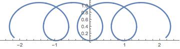
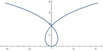
Figure 1: Invariant $\lambda$-translating solitons for $\lambda=1$ (left) and $\lambda=1/2$ (right). Here $\vec{v}=(0,0,1)$ and the initial condition is $\theta(0)=0$

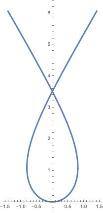
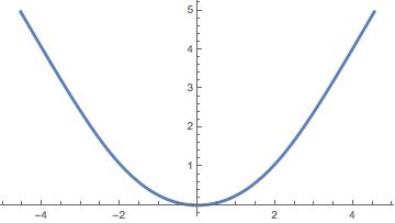
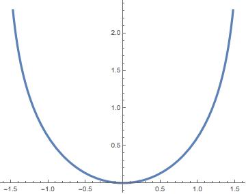
Figure 2: Left and middle: invariant $\lambda$-translating solitons for $\lambda=1/4$ and initial condition $\theta_{0}=0$ and $\theta_{0}=\pi$, respectively. Right: the grim reaper. Here $\vec{v}=(0,0,1)$

Remark 2.5.

By Prop. 2.1 and Th. 2.4, the only cases where a $\lambda$-translating soliton of cylindrical type is a graph on a planar domain are the grim reaper ($\lambda=0$), which is a graph on a strip, and the case $\lambda\in(0,v_{3}/2)$, where the surface is an entire graph. In both cases, the graph is convex.

We finish this section indicating that it is possible to integrate explicitly (4). The third equation in (4) is

$$\int\frac{d\theta}{2\lambda+v_{3}\cos\theta}=s+a,\ a\in\mathbb{R}.$$

Then the change $u=\tan(\theta/2)$ gives, up to a linear change in the parameter $s$,

$$\theta(s)=\left\{\begin{array}[]{ll}2\arctan\left(\sqrt{\frac{2\lambda+v_{3}}{2\lambda-v_{3}}}\tan\left(\frac{\sqrt{4\lambda^{2}-v_{3}^{2}}}{2}s\right)\right)&\lambda>\frac{v_{3}}{2}\\ 2\arctan(v_{3}s)&\lambda=\frac{v_{3}}{2}\\ 2\arctan\left(\sqrt{\frac{2\lambda+v_{3}}{-2\lambda+v_{3}}}\tanh\left(\frac{\sqrt{v_{3}^{2}-4\lambda^{2}}}{2}s\right)\right)&0<\lambda<\frac{v_{3}}{2}\end{array}\right.$$

Once obtained the function $\theta$, we compute $\cos\theta$ and $\sin\theta$ in order to solve the functions $y$ and $z$ in (4). This can be only done in those intervals where is defined the $\arctan$ function. The explicit integration gives:

Theorem 2.6.

The generating curve $\alpha(s)=(y(s),z(s))$ of a cylindrical $\lambda$-translating soliton $X(s,t)=(t,y(s),z(s))$, $s\in I$, $t\in{\mathbb{R}}$ is:

1. Case $\lambda>v_{3}/2$.

   $$y(s)=-2\lambda s+2\arctan\left(\frac{2\lambda+v_{3}}{\sqrt{4\lambda^{2}-v_{3}}}\tan(\frac{\sqrt{4\lambda^{2}-v_{3}^{2}}}{2}s)\right)$$

   $$z(s)=\log\left|2\lambda-\cos(\sqrt{4\lambda^{2}-v_{3}^{2}}s)\right|.$$

2. Case $\lambda=v_{3}/2$.

   $$\alpha(s)=\left(-s+\frac{2}{v_{3}}\arctan(v_{3}s),\frac{1}{v_{3}}\log|1+s^{2}v_{3}^{2}|\right).$$

3. Case $0<\lambda<v_{3}/2$.

   $$y(s)=-2\lambda s+2\arctan\left(\frac{2\lambda+v_{3}}{\sqrt{v_{3}^{2}-4\lambda^{2}}}\tanh(\frac{\sqrt{v_{3}^{2}-4\lambda^{2}}}{2}s)\right)$$

   $$z(s)=\log\left|-2\lambda+\cosh(\sqrt{v_{3}^{2}-4\lambda^{2}}s)\right|.$$

4. Case $\lambda=0$ (grim reaper).

   $$\alpha(s)=\left(2\arctan(\tanh(\frac{s}{2})),\log(\cosh(s))\right).$$

3 Translating solitons of translation type

The parametrization $X(s,t)=\alpha(s)+t\vec{a}$ of a cylindrical surface allows to see the surface as the sum of two planar curves, namely, $X(s,t)=\alpha(s)+\beta(t)$, where $\beta$ is the straight line $\beta(t)=t\vec{a}$. More generally, we can consider the solutions of (1) that are the sum of two planar curves $\alpha(x)=(x,0,f(x))$ and $\beta(y)=(0,y,g(y))$. The parametrization $X(x,y)=(x,y,f(x)+g(y))$ is noting that the surface in the non-parametric form $z=f(x)+g(y)$. A such surface is called a translation surface and in this section we investigate the solutions of (1) that are translation surfaces. For translating solitons $(\lambda=0)$ and when the density vector is orthogonal to the $xy$-plane, it is known that the only translating solitons of translation type are cylindrical surfaces ([11]). Exactly, and besides the plane, the functions $f$ and $g$ are, up to a change of the roles of $f$ and $g$, $f(x)=ax+b$ and

$$g(y)=-(1+a^{2})\log\left|\cos\left(\frac{x}{\sqrt{1+a^{2}}}\right)\right|,$$

where $a,b\in\mathbb{R}$. The surface for $a=0$ is the grim reaper. When $\vec{v}$ is not orthogonal to the $xy$-plane, there exist many examples of translating solitons $z=f(x)+g(y)$ ([9]).

In this section, we find all $\lambda$-translating solitons of translation type when the density vector $\vec{v}$ takes all its generality.

Theorem 3.1.

Let $\vec{v}=(v_{1},v_{2},v_{3})$ be the density vector. The only $\lambda$-translating solitons $z=f(x)+g(y)$ are:

1. Planes and $f$ and $g$ are linear functions.

2. Up to a change of the roles of $f$ and $g$, we have $f(x)=ax+b$, and $g$ satisfies

   $$(1+a^{2})g^{\prime\prime}=2\lambda(1+a^{2}+g^{\prime 2})^{3/2}+(1+a^{2}+g^{\prime 2})(-v_{1}a-v_{2}g^{\prime}+v_{3}),$$ (6)

   where $a,b\in\mathbb{R}$. In particular, the surface is cylindrical and the rulings are parallel to the vector $(1,0,a)$.

Proof.

The case $\lambda=0$ was studied in [9, 11]. Consider now $\lambda\not=0$. Using the parametrization $X(x,y)=(x,y,f(x)+g(y))$, with $(x,y)\in I\times J\subset\mathbb{R}^{2}$, the Gauss map is

$$\langle N,\vec{v}\rangle=\frac{-v_{1}f^{\prime}-v_{2}g^{\prime}+v_{3}}{W^{1/2}},$$

where $W=1+f^{\prime 2}+g^{\prime 2}$. Then Eq. (1) is

$$\frac{(1+g^{\prime 2})f^{\prime\prime}+(1+f^{\prime 2})g^{\prime\prime}}{W^{3/2}}=2\lambda+\frac{-v_{1}f^{\prime}-v_{2}g^{\prime}+v_{3}}{W^{1/2}}.$$ (7)

Multiplying by $W^{3/2}$ and differentiating with respect to $x$, next with respect to $y$ and simplifying, we get

$$g^{\prime}g^{\prime\prime}f^{\prime\prime\prime}+f^{\prime}f^{\prime\prime}g^{\prime\prime\prime}=3\lambda\frac{f^{\prime}f^{\prime\prime}g^{\prime}g^{\prime\prime}}{W^{1/2}}-(v_{1}f^{\prime\prime}g^{\prime}g^{\prime\prime}+v_{2}f^{\prime}f^{\prime\prime}g^{\prime\prime}).$$ (8)

Suppose that at some $(x_{0},y_{0})\in I\times J$ we have $f^{\prime}f^{\prime\prime}(x_{0})g^{\prime}g^{\prime\prime}(y_{0})\not=0$. By continuity, in some open set around $(x_{0},y_{0})$, we have $f^{\prime}f^{\prime\prime}g^{\prime}g^{\prime\prime}\not=0$. Dividing (8) by $f^{\prime}f^{\prime\prime}g^{\prime}g^{\prime\prime}$, we obtain

$$\frac{f^{\prime\prime\prime}}{f^{\prime}f^{\prime\prime}}+\frac{g^{\prime\prime\prime}}{g^{\prime}g^{\prime\prime}}+\frac{v_{1}}{f^{\prime}}+\frac{v_{2}}{g^{\prime}}=\frac{3\lambda}{W^{1/2}}.$$

Since the left hand side is the sum of a function on $x$ and a function on $y$, when we differentiate with respect to $x$ and next with respect to $y$, the left hand side vanishes. Doing the same differentiations in the right hand side, we get

$$0=9\lambda\frac{f^{\prime}f^{\prime\prime}g^{\prime}g^{\prime\prime}}{W^{5/2}},$$

obtaining a contradiction because $\lambda\not=0$. The above argument proves $f^{\prime}f^{\prime\prime}g^{\prime}g^{\prime\prime}=0$ in $I\times J$. Without loss of generality, and by the symmetry of the roles of $f$ and $g$, we suppose $f^{\prime}f^{\prime\prime}=0$ in the interval $I$. If at some point $x_{0}\in I$, we have $f^{\prime}(x_{0})\not=0$, then $f^{\prime\prime}=0$ around $x_{0}$, that is, $f(x)=ax+b$, $a,b\in\mathbb{R}$. With this function $f$, Eq. (7) reduces into (6), obtaining the result. In the case that $f^{\prime}=0$, then $f^{\prime\prime}=0$, concluding the same result. ∎

We finish this section showing two examples of $\lambda$-translating solitons of translation type with $\lambda\not=0$.

1. Consider the density vector to be $\vec{v}=(0,0,1)$. Take $f(x)=0$ and $\lambda=1$ in (6). Then $g$ satisfies $g^{\prime\prime}=1+g^{\prime 2}+2(1+g^{\prime 2})^{3/2}$. This surface appears in Th. 2.4, item 1

2. Consider $\vec{v}=(1,0,0)$ as the density vector. Take $f(x)=0$. Then Eq. (6) is $g^{\prime\prime}=2\lambda(1+g^{\prime 2})^{3/2}$ whose solution is

   $$g(y)=\frac{\sqrt{1-4\lambda^{2}y^{2}}}{2\lambda},$$

   that is, $y=g(y)$ describes a circle of radius $1/(2|\lambda|)$ and the surface is a circular right cylinder whose axis is $\vec{v}$. This solution appeared in Prop. 2.1.

4 Rotational $\lambda$-translating solitons

In this section, we classify all rotational surfaces that are $\lambda$-translating solitons. First examples are a plane orthogonal to $\vec{v}$ and a right circular cylinder with axis parallel to $\vec{v}$. In the particular case $\lambda=0$, the translating solitons of rotational type were studied in [2], obtaining two types of surfaces, namely, the paraboloid bowl soliton and a family of rotationally surfaces of winglike shape.

Our interest is also those solutions with a particular geometry as for example, when the surface meets the rotation axis or if it is embedded. A first question is about the existence of closed surfaces. Let us recall that the round sphere is the only rotational constant mean curvature surface that is closed and that there are many examples of closed surfaces with constant mean curvature which are not rotational. However, for $\lambda$-translating solitons we have:

Theorem 4.1.

There are no closed $\lambda$-translating solitons.

Proof.

By contradiction, let $\psi:\Sigma\rightarrow\mathbb{R}^{3}$ be an immersion of a closed surface $\Sigma$ whose mean curvature $H$ satisfies (1). It is known that if $\vec{a}\in\mathbb{R}^{3}$, the Laplacian $\Delta$ of the height function $\langle\psi,\vec{a}\rangle$ is $\Delta\langle\psi,\vec{a}\rangle=2H\langle N,\vec{a}\rangle$. If we take $\vec{a}=\vec{v}$, we have

$$\Delta\langle\psi,\vec{v}\rangle=2\lambda\langle N,\vec{v}\rangle+\langle N,\vec{v}\rangle^{2}.$$ (9)

We integrate this identity in $\Sigma$. By using the divergence theorem and because $\partial\Sigma=\emptyset$, we have

$$0=2\lambda\int_{\Sigma}\langle N,\vec{v}\rangle\ d\Sigma+\int_{\Sigma}\langle N,\vec{v}\rangle^{2}\ d\Sigma.$$ (10)

On the other hand, the constant vector field in $\mathbb{R}^{3}$ defined by $Y(p)=\vec{v}$ has zero divergence and thus the divergence theorem gives now $\int_{\Sigma}\langle N,\vec{v}\rangle\ d\Sigma=0$. We conclude from (10) that $0=\int_{\Sigma}\langle N,\vec{v}\rangle^{2}\ d\Sigma$, that is, $\Sigma$ is included in a plane parallel to $\vec{v}$, a contradiction. ∎

Remark 4.2.

In the literature, the proof of Th. 4.1 for translating solitons ($\lambda=0$) uses the maximum principle for (1) and an argument of comparison with planes parallel to $\vec{v}$. However, this proof fails if $\lambda\not=0$. In contrast, the proof given in Th. 4.1 is simpler because only uses the divergence theorem and it holds for any $\lambda$.

Although in our initial study there is not an a priori relation between the rotational axis and the density vector, we prove that they must be parallel.

Proposition 4.3.

Let $\Sigma$ be a rotational surface about the axis $L$. If $\Sigma$ is a $\lambda$-translating soliton with density vector $\vec{v}$, then $\vec{v}$ and $L$ are parallel or $\Sigma$ is a plane orthogonal to $L$ and $\vec{v}$.

Proof.

After a change of coordinates, we suppose that the rotational axis is the $z$-axis. A parametrization of $\Sigma$ is $X(s,t)=(x(s)\cos t,x(s)\sin t,z(s))$, $s\in I$, $t\in\mathbb{R}$, where $\alpha(s)=(x(s),0,z(s))$, $x(s)>0$, is the profile curve which we suppose is parametrized by the arc-length. Let $x^{\prime}(s)=\cos\theta(s)$, $z^{\prime}(s)=\sin\theta(s)$ for some function $\theta$. If $\vec{v}=(v_{1},v_{2},v_{3})$, then Eq. (1) is

$$\frac{\sin\theta}{x}+\theta^{\prime}=2\lambda-v_{1}\sin\theta\cos t-v_{2}\sin\theta\sin t+v_{3}\cos\theta,$$

for all $s\in I,t\in\mathbb{R}$. Since the functions $\{\cos t,\sin t,1\}$ are independent linearly, we deduce

$$v_{1}\sin\theta(s)=v_{2}\sin\theta(s)=0$$

for all $s\in I$. If there exists $s_{0}\in I$ such that $\sin\theta(s_{0})\not=0$, then $v_{1}=v_{2}=0$ and $\vec{v}$ is parallel to the $z$-axis, proving the result. On the contrary, the function $\sin\theta$ is identically $0$ in the interval $I$. This means that $\alpha$ is a horizontal line and $\Sigma$ is a horizontal plane: now the density vector $\vec{v}$ is arbitrary. ∎

As a consequence of Prop. 4.3 and without loss of generality, we suppose that the rotational axis is the $z$-axis and $\vec{v}=(0,0,1)$. As before, if $\alpha(s)=(x(s),0,z(s))$ is the profile curve, then the functions $x$, $z$ and $\theta$ satisfy

$$\left\{\begin{array}[]{lll}x^{\prime}(s)&=&\cos\theta(s)\\ z^{\prime}(s)&=&\sin\theta(s)\\ \theta^{\prime}(s)&=&\displaystyle 2\lambda+\cos\theta(s)-\frac{\sin\theta(s)}{x(s)}.\end{array}\right.$$ (11)

A particular case of (11) appears when $\theta$ is a constant function. Then $\alpha$ is a straight line and $2\lambda+\cos\theta+\sin\theta/x(s)=0$. From the first equation in (11), we know $x(s)=a+(\cos\theta)s$, $a\in\mathbb{R}$, and substituting in the third equation of (11), we have

$$\cos\theta(2\lambda+\cos\theta)s+2\lambda a+a\cos\theta-\sin\theta=0.$$

Since this is a polynomial equation on the variable $s$, we deduce

$$\cos\theta(2\lambda+\cos\theta)=0,\quad 2\lambda a+a\cos\theta-\sin\theta=0.$$ (12)

If $\cos\theta=0$, then $\alpha$ is the vertical line of equation $x=1/(2|\lambda|)$ and the surface is a right circular cylinder. If $\cos\theta\not=0$, we have from (12) that $\sin\theta=0$ and thus $\alpha$ is a horizontal line and $\Sigma$ is a horizontal plane. Therefore we have proved the next result:

Proposition 4.4.

The only rotational $\lambda$-translating solitons generated by straight lines are planes and right circular cylinders of radius $1/(2|\lambda|)$.

We give now the relationship between the shape of a rotational $\lambda$-translating soliton and the sign of $\lambda$. After a vertical translation, we take the initial conditions

$$x(0)=x_{0}>0,\ \ z(0)=0,\ \ \theta(0)=\theta_{0},$$ (13)

and denote $x(s;\lambda,\theta_{0}),\ z(s;\lambda,\theta_{0}),\ \theta(s;\lambda,\theta_{0})$ the solutions of (11) with initial conditions (13) depending on $\theta_{0}$. The next result is analogous to Prop. 2.3.

Proposition 4.5.

For suitable initial conditions in (13), the graphic of a solution of (11) for $\lambda$ coincides with the graphic of a solution of (11) for $-\lambda$ and we have

$$(x(s;\lambda,\theta_{0}),z(s;\lambda,\theta_{0}))=(x(-s;-\lambda,\theta_{0}+\pi),z(-s;-\lambda,\theta_{0}+\pi)),\ s\in\mathbb{R}.$$

Proof.

The proof is analogous to Prop. 2.3 by defining the functions

$$\bar{x}(s) = x(-s;-\lambda,\theta_{0}+\pi)$$

$$\bar{z}(s) = z(-s;-\lambda,\theta_{0}+\pi)$$

$$\bar{\theta}(s) = \theta(-s;-\lambda,\theta_{0}+\pi)+\pi.$$

∎

We come back to the ODE system (11). Multiplying the third equation by $x(s)$, we have $x\theta^{\prime}=2\lambda x+xx^{\prime}-z^{\prime}$ and thus

$$(x\sin\theta)^{\prime}=x^{\prime}z^{\prime}+\cos\theta x\theta^{\prime}=x^{\prime}z^{\prime}+\cos\theta(2\lambda x+xx^{\prime}-z^{\prime})=(\lambda x^{2})^{\prime}+xx^{\prime 2}.$$

If we fix $s_{0}\in I$, then

$$x(s)\sin\theta(s)-\lambda x(s)^{2}=x(s_{0})\sin\theta(s_{0})-\lambda x(s_{0})^{2}+\int_{s_{0}}^{s}x(t)x^{\prime}(t)^{2}dt.$$ (14)

We prove that if the graphic of $\alpha$ meets the rotational axis, then this intersection is orthogonal.

Proposition 4.6.

If the profile curve of a rotational $\lambda$-translating soliton intersects the rotational axis, then it does so at a perpendicular angle.

Proof.

Without loss of generality, suppose that the intersection between the curve and the axis occurs at $s=0$. Then $x(0)=0$ and from (14), we have

$$x(s)\sin\theta(s)-\lambda x(s)^{2}=\int_{0}^{s}x(t)x^{\prime}(t)^{2}dt.$$ (15)

We divide this expression by $x(s)$, obtaining

$$\sin\theta(s)-\lambda x(s)=\frac{1}{x(s)}\int_{0}^{s}x(t)x^{\prime}(t)^{2}dt.$$

Letting $s\rightarrow 0$ and applying the L’Hôpital rule, we obtain

$$\sin\theta(0)=\frac{x(0)x^{\prime}(0)^{2}}{x^{\prime}(0)}=x(0)x^{\prime}(0)=0,$$

and this proves the result. ∎

We study the existence of solutions of (11)-(13). The local existence is assured if $x(0)>0$. When $x(0)=0$, the third equation in (11) presents a singularity and thus the existence is not a direct consequence of the standard theory. We study this case. By Props. 4.5 and 4.6, the initial condition for $\theta$ is $\theta(0)=0$. We give a proof of the existence using known techniques of the theory of the radial solutions for an elliptic equation. Here we prefer to write (1) (or (11)) as the prescribed mean curvature equation

$$\frac{u^{\prime\prime}(r)}{(1+u^{\prime}(r)^{2})^{3/2}}+\frac{u^{\prime}(r)}{r\sqrt{1+u^{\prime}(r)^{2}}}=2H=2\lambda+\frac{1}{\sqrt{1+u^{\prime}(r)^{2}}},$$ (16)

where, as usually, $r$ is the radial variable and $u=u(r)$. Multiplying (16) by $r$, we want to establish the existence of a classical solution of

$$\left\{\begin{array}[]{ll}\left({\displaystyle\frac{ru^{\prime}(r)}{\sqrt{1+u^{\prime}(r)^{2}}}}\right)^{\prime}=2\lambda r+{\displaystyle\frac{r}{\sqrt{1+u^{\prime}(r)^{2}}}},&\mbox{ in $(r_{0},r_{0}+\delta)$}\\ u(r_{0})=0,\quad u^{\prime}(r_{0})=0&\end{array}\right.$$ (17)

where $r_{0}\geq 0$. We consider the case $r_{0}=0$, where Eq. (17) is degenerate.

Proposition 4.7.

The initial value problem (17) with $r_{0}=0$ has a solution $u\in C^{2}([0,R])$ for some $R>0$ which depends continuously on the initial datum.

Proof.

Define the functions $g:\mathbb{R}_{0}^{+}\times\mathbb{R}\rightarrow\mathbb{R}$ and $\varphi:\mathbb{R}\rightarrow\mathbb{R}$ by

$$g(x,y)=2\lambda+\frac{1}{\sqrt{1+y^{2}}},\ \varphi(y)=\frac{y}{\sqrt{1+y^{2}}}.$$

It is clear that a function $u\in C^{2}([0,\delta])$, for some $\delta>0$, is a solution of (17) if and only if $rg(u,u^{\prime})=(r\varphi(u^{\prime}))^{\prime}$ and $u(0)=0$, $u^{\prime}(0)=0$.

Fix $\delta>0$ to be determined later and define the operator ${\mathcal{S}}$ by

$$({\mathcal{S}}u)(r)=a+\int_{0}^{r}\varphi^{-1}\left(\int_{0}^{s}\frac{t}{s}\left(2\lambda+\frac{1}{\sqrt{1+u^{\prime 2}}}\right)dt\right)ds.$$

Then a fixed point of the operator ${\mathcal{S}}$ is a solution of the initial value problem (17). We prove that ${\mathcal{S}}$ is a contraction in the space $C^{1}([0,\delta])$ endowed the usual norm $\|u\|=\|u\|_{\infty}+\|u^{\prime}\|_{\infty}$. The functions $g$ and $\varphi^{-1}$ are Lipschitz continuous of constant $L>0$ in $[-\epsilon,\epsilon]\times[-\epsilon,\epsilon]$ and $[-\epsilon,\epsilon]$, respectively provided $\epsilon>0$ and $\epsilon<1$. Then for all $u,v\in\overline{B(0,\epsilon)}$ and for all $r\in[0,\delta]$,

$$|({\mathcal{S}}u)(r)-({\mathcal{S}}v)(r)|\leq\frac{L^{2}}{4}r^{2}\left(\|u-v\|_{\infty}+\|u^{\prime}-v^{\prime}\|_{\infty}\right)$$

$$|({\mathcal{S}}u)^{\prime}(r)-({\mathcal{S}}v)^{\prime}(r)|\leq\frac{L^{2}}{2}r\left(\|u-v\|_{\infty}+\|u^{\prime}-v^{\prime}\|_{\infty}\right)$$

Hence choosing $\delta>0$ small enough, we conclude that ${\mathcal{S}}$ is a contraction in the closed ball $\overline{B(0,\delta)}$ in $C^{1}([0,\delta])$. Thus the Schauder Point Fixed theorem proves the existence of a local solution of the initial value problem (17). This solution lies in $C^{1}([0,\delta])\cap C^{2}(0,\delta])$ and the $C^{2}$-regularity up to $0$ is verified directly by using the L’Hôpital rule: from (16) we have

$$u^{\prime\prime}(0)+\lim_{r\rightarrow 0}\frac{u(r)}{r}=2\lambda+1,$$

that is,

$$\lim_{r\rightarrow 0}u^{\prime\prime}(r)=\lambda+\frac{1}{2}.$$

The continuous dependence of local solutions on the initial datum is a consequence of the continuous dependence of the fixed points of ${\mathcal{S}}$. ∎

In a first step of the classification of the rotational $\lambda$-translating solitons, we study the solutions of (11) that intersect orthogonally the rotational axis. This means $x_{0}=\theta_{0}=0$ in (13). We write here the third equation of (11), namely,

$$\theta^{\prime}(s)=2\lambda+\cos\theta(s)-\frac{\sin\theta(s)}{x(s)}.$$ (18)

As first observations, we have:

1. The monotonicity of the angle function $\theta$ close to $s=0$ is given by the value $\theta^{\prime}(0)$. Equation (18) and the L’Hôpital rule gives $\theta^{\prime}(0)=\lambda+1/2$. Therefore $\theta$ is increasing (resp. decreasing) around $s=0$ if $\lambda>-1/2$ (resp. $\lambda<-1/2$).

2. If $\lambda>0$, from (15) we deduce that $\theta$ does not attain the value $\pi$. Similarly, the function $\theta$ does not attain again the value $0$ because if $s_{1}>0$ is the first time where $\theta(s_{1})=0$, then $\theta^{\prime}(s_{1})\leq 0$, but (11) gives $\theta^{\prime}(s_{1})=2\lambda+1>0$. This contradiction proves that $\theta$ is a bounded function $0<\theta(s)<\pi$. In particular, the solutions of (11) are defined in $(0,\infty)$. Moreover, from (15) again, $x(s)-\lambda x(s)^{2}>0$ for every $s$ and we deduce that the function $x(s)$ is bounded, namely, $x(s)<1/\lambda$.

3. If $\lambda=0$, then the surface is the bow soliton ([2]).

4. If $\lambda=-1/2$, then it is immediate that the solution of (11)-(13) for $x_{0}=\theta_{0}=0$ is $x(s)=s$, $z(s)=0$ and $\theta(s)=0$, that is, $\alpha$ is a horizontal line and the surface is a horizontal plane.

From now we discard the case $\lambda=0$. In order to give a description of the profiles curves, we do an analytic study of the solutions of (11) from the viewpoint of the dynamic system theory. Here we follow a similar study done by Gomes in [4] in the classification of the rotational surfaces of spherical type with constant mean curvature in hyperbolic space ${\mathbb{H}}^{3}$ (see also [3] for other types of rotational surfaces in ${\mathbb{H}}^{3}$ and the Euclidean case). We project the vector field $(x^{\prime}(s),z^{\prime}(s),\theta^{\prime}(s))$ on the $(\theta,x)$ plane, obtaining the one-parameter plane vector field

$$\left\{\begin{array}[]{lll}\theta^{\prime}(s)&=&\displaystyle 2\lambda+\cos\theta(s)-\frac{\sin\theta(s)}{x(s)},\\ x^{\prime}(s)&=&\cos\theta(s).\end{array}\right.$$

Multiplying the vector field $(\theta,x)$ by $x$, which is positive, to eliminate the poles, we conclude that the above system is equivalent to the next autonomous system

$$\left\{\begin{array}[]{lll}\theta^{\prime}(s)&=&\displaystyle 2\lambda x(s)+x(s)\cos\theta(s)-\sin\theta(s)\\ x^{\prime}(s)&=&x(s)\cos\theta(s).\end{array}\right.$$ (19)

We study the qualitative properties of the solutions of (19). By the periodicity of the functions $\sin\theta$ and $\cos\theta$, it suffices to consider $\theta\in[-\pi,\pi]$. In the region $[-\pi,\pi]\times\{(\theta,x):x\geq 0\}$, the singularities of the vector field $V(\theta,x)=(2\lambda x+x\cos\theta-\sin\theta,x\cos\theta)$ are the points $P_{1}=(0,0)$, $P_{2}=(\pi,0)$, $P_{3}=(-\pi,0)$ and, furthermore, the point $Q_{1}=(\pi/2,1/(2\lambda))$ in case $\lambda>0$, and the point $Q_{2}=(-\pi/2,-1/(2\lambda))$ if $\lambda<0$. We study the type of critical point in all these cases. The linearization of $V$ is

$$LV(\theta,x)=\left(\begin{array}[]{cc}-x\sin\theta-\cos\theta&2\lambda+\cos\theta\\ -x\sin\theta&\cos\theta\end{array}\right),$$

and denote $\mu_{1}$ and $\mu_{2}$ the two eigenvalues. The critical points $P_{i}$ are hyperbolic because the eigenvalues of $LV(P_{i})$ are real with $\mu_{1}<0<\mu_{2}$. For the points $Q_{i}$, the eigenvalues $\mu_{1}$ and $\mu_{2}$ are $(-1\pm\sqrt{1-16\lambda^{2}})/(4\lambda)$ and the types of singularities appear in Tables 1 and 2.

$Q_{1}$	$0<\lambda<1/4$	$\lambda=1/4$	$\lambda>1/4$
eigenvalues	$\mu_{1}<\mu_{2}<0$	$\mu_{1}=\mu_{2}<0$	$\Re(\mu_{i})<0$
type	stable node	stable improper node	stable spiral point

Table 1: Types of singularity at $Q_{1}$

$Q_{2}$	$-1/4<\lambda<0$	$\lambda=-1/4$	$\lambda<-1/4$
eigenvalues	$\mu_{1}>\mu_{2}>0$	$\mu_{1}=\mu_{2}>0$	$\Re(\mu_{i})>0$
type	unstable node	unstable improper node	unstable spiral point

Table 2: Types of singularity at $Q_{2}$

We analyze the different cases of rotational surfaces depending on the value of $\lambda$.

1. Case $\lambda>1/4$.

   If $\lambda>1/4$, then $\theta^{\prime}(0)=\lambda+1/2>0$ and this means that $\theta$ is increasing in a neighbourhood of $s=0$. We know that the point $Q_{1}=(\pi/2,1/(2\lambda))$ is a stable spiral point. Therefore, and by the phase portrait (Fig. 3, left), the angle function $\theta$ is increasing in a first moment, next $\theta$ crosses the value $\pi/2$, and next decreases crossing $\pi/2$ again. This behavior is repeating as $\theta\rightarrow\pi/2$: see Fig. 3, right. On the other hand, the function $x$ is bounded with $x<1/\lambda$ and oscillating around the value $1/(2\lambda)$ as $s\rightarrow\infty$, being this value its limit. Since $\theta\rightarrow\pi/2$, then $z^{\prime}(s)=\sin\theta\rightarrow 1$ and the function $z$ increasing towards $\infty$.

   We have proved that the profile curve is an embedded curve converging to the vertical line $x=1/(2\lambda)$ and crossing this line infinitely times.

   

   

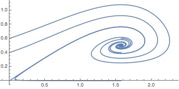
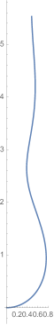
   Figure 3: Rotational surfaces for $\lambda>1/4$. Here $\lambda=1$. Left: the phase portrait around $Q_{1}$. Right: the profile curve intersecting the rotational axis

2. Case $\lambda=1/4$.

   The singularity $Q_{1}$ is a stable improper node. As in the above case, $\theta$ is increasing for $s>0$ and we have again $\theta\rightarrow\pi/2$, $x(s)\rightarrow 1/(2\lambda)$ and $z(s)\rightarrow\infty$. The profile curve is embedded converging to the vertical line of equation $x=1/(2\lambda)$.

3. Case $0<\lambda<1/4$.

   The function $\theta$ is increasing again in a neighbourhood of $s=0$. Since $Q_{1}$ is a stable node, the function $\theta$ does not attain the value $\pi/2$ (Fig. 4, left). Then $\theta$ is increasing in its domain: on the contrary, at the first point $s_{1}$ where $\theta$ decreases, we have $\theta^{\prime}(s_{1})=0$ and $\theta^{\prime\prime}(s_{1})\leq 0$, but

   $$\theta^{\prime\prime}(s_{1})=-\theta^{\prime}(s_{1})\left(\sin\theta(s_{1})+\frac{\cos\theta(s_{1})}{x(s_{1})}\right)+\frac{\sin\theta(s_{1})\cos\theta(s_{1})}{x(s_{1})^{2}}>0.$$ (20)

   Thus $\theta$ is increasing with $\theta\rightarrow\pi/2$. This proves that $\alpha$ is a graph on the $x$-line with $x(s)$ an increasing function and $x(s)\rightarrow 1/(2\lambda)$. Since $\theta^{\prime}(s)>0$, the graph of $\alpha$ is convex on the $x$-interval $[0,1/(2\lambda))$: see Fig. 4, right.

   

   

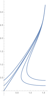
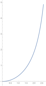
   Figure 4: Rotational surfaces for $0<\lambda<1/4$. Here $\lambda=0.15$. Left: the phase portrait. Right: the profile curve intersecting the rotational axis

4. Case $-1/2<\lambda<0$.

   As $\theta^{\prime}(0)=\lambda+1/2>0$, we know that $\theta$ is increasing around $s=0$. We prove that $\alpha$ is a graph on the $x$-line. If there exists a first point $s_{1}>0$ such that $\alpha^{\prime}(s_{1})$ is vertical, then we have two possibilities. If $\theta(s_{1})=\pi/2$, then $\theta^{\prime}(s_{1})\geq 0$, but from (18), we have $\theta^{\prime}(s_{1})=2\lambda-1/x(s_{1})<0$. This implies that $\theta(s_{1})=-\pi/2$ and $\theta^{\prime}(s_{1})\leq 0$, in particular, there exists $s_{0}\in(0,s_{1})$ with $\theta(s_{1})\in(0,\pi/2)$ such that $\theta^{\prime}(s_{0})=0$ and $\theta^{\prime\prime}(s_{0})\leq 0$. However, as in (20), we have $\theta^{\prime\prime}(s_{1})>0$. This contradiction proves that $\alpha$ is a graph and $\theta$ is as increasing function with $0<\theta(s)<\pi/2$ and since $\theta^{\prime}>0$, then $\alpha$ is convex. In particular, the singularity $Q_{2}=(-\pi/2,-1/(2\lambda))$ is not attained as $s\rightarrow\infty$: see Fig. 5, left.

   Finally, we show that function $x$ is not bounded (Fig. 5, right). As $x^{\prime}(s)=\cos\theta(s)>0$, then $x=x(s)$ is increasing. If $x$ is bounded, then $x^{\prime}(s)\rightarrow 0$ and $x(s)\rightarrow\bar{x}$ for some positive number $\bar{x}$. Then $\theta\rightarrow\pi/2$ as $s\rightarrow\infty$. Letting $s\rightarrow\infty$ in (18), we get $0=2\lambda-1/\bar{x}$, a contradiction because $\lambda<0$. Definitively, $\alpha$ is a convex graph on $(0,\infty)$.

   

   

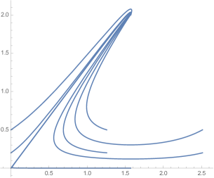
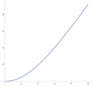
   Figure 5: Rotational surfaces for $-1/2<\lambda<0$. Here $\lambda=-0.25$. Left: the phase portrait around $Q_{2}$. Right: the profile curve intersecting the rotational axis

5. Case $\lambda<-1/2$.

   As $\theta^{\prime}(0)=2\lambda+1<0$, the function $\theta$ is initially decreasing, in particular, $x$ is increasing. Now the point $Q_{2}=(-\pi/2,-1/(2\lambda))$ is an unstable spiral point with respect to it, the trajectories curl anti-clockwise towards infinity (Fig. 6, left). In particular, we have $\theta(s)\rightarrow-\infty$ and $x(s)\rightarrow\infty$. This implies that $\alpha$ is a curve that self-intersects and curls clockwise to infinity (Fig. 6, right).

   

   

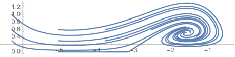
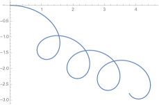
   Figure 6: Rotational surfaces for $\lambda<-1/2$. Here $\lambda=-1$. Left: the phase portrait around $Q_{2}$. Right: the profile curve intersecting the rotational axis

We summarize in the next result.

Theorem 4.8.

We have the next classification of rotational $\lambda$-translating solitons that intersect the rotational axis. Without loss of generality, we suppose that the rotational axis is the $z$-axis and the density vector is $(0,0,1)$. Denote $C_{\lambda}$ the right vertical cylinder of radius $1/(2|\lambda|)$.

1. Case $\lambda\geq 1/4$. The surface is embedded and asymptotic to $C_{\lambda}$.

2. Case $0<\lambda<1/4$. The surface is a convex graph on a disc of radius $1/(2\lambda)$ and asymptotic to $C_{\lambda}$.

3. Case $\lambda=0$. The surface is the bow soliton.

4. Case $-1/2<\lambda<0$. The surface is a convex entire graph on the $xy$-plane.

5. Case $\lambda=-1/2$. The surface is a horizontal plane.

6. Case $\lambda<-1/2$. The surface has infinity self-intersections.

We end this section obtaining the classification of the rotational $\lambda$-translating solitons that do not intersect the rotational axis. We consider the solution $(x,z,\theta)$ of (11) with initial conditions $x(0)=x_{0}>0$ and $\theta(0)=\theta_{0}$. Since the solution is also defined for negative values of $s$, by Prop. 4.5 the solution in the interval $(-\infty,0)$ coincides with the solution of (11) for the value $-\lambda$ and initial conditions $x(0)=x_{0}$ and $\theta(0)=\theta_{0}+\pi$. As $s\rightarrow\infty$, the behavior of the profile curve is as in Th. 4.8 according to the trajectories of (19) . When $s\rightarrow-\infty$, the singularity $Q_{2}$ is attained when $\lambda<0$. In the next result, we distinguish case-by-case depending on the value of $\lambda$, where the first statement refers when $s\rightarrow\infty$ in the profile curve (positive branch) and the second statement when $s\rightarrow-\infty$ (negative branch). Thus we deduce from Th. 4.8:

Theorem 4.9.

We have the next classification of rotational $\lambda$-translating solitons that do not intersect the rotational axis. Without loss of generality, we suppose that the rotational axis is the $z$-axis and the density vector is $(0,0,1)$. Denote $C_{\lambda}$ the right vertical cylinder of radius $1/(2|\lambda|)$.

1. For each $\lambda$, the cylinder $C_{\lambda}$.

2. Case $\lambda>1/4$. The surface has two ends, one end is embedded and asymptotic to $C_{\lambda}$ and the other end has infinity self-intersections.

3. Case $0<\lambda\leq 1/4$. The surface has two embedded ends, one end is asymptotic to $C_{\lambda}$ and the other one is a convex graph on the compliment of a round disc of the $xy$-plane.

4. Case $\lambda=0$. The surface is the winglike-surface translating soliton ([2]).

5. Case $-1/2\leq\lambda<0$. The surface has two embedded ends, one end is a convex graph on the compliment of a round disc of the $xy$-plane and the other end is asymptotic to $C_{\lambda}$.

6. Case $\lambda<-1/2$. The surface has one end with infinity self-intersections and the other end is embedded and asymptotic to $C_{\lambda}$.

Some examples of rotational $\lambda$-translating solitons that do not intersect the rotational axis appear in Fig. 7

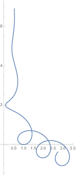
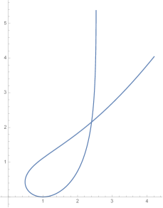
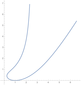
Figure 7: Rotational $\lambda$-translating solitons that do no intersect the rotational axis. Left: $\lambda=1$. Middle: $\lambda=0.2$. Right: An embedded rotational $1/4$-translating soliton that does not intersect the rotational axis and the initial condition is $\theta(0)=\pi$

From the above classification we ask if among these surfaces, and besides the cylinders $C_{\lambda}$, there are embedded examples. We have to consider $\theta(0)=\theta_{0}$ inall its generality by taking any value in an interval of length $2\pi$. If $\lambda>1/4$ or $\lambda<-1/2$, then it is clear that the angle function $\theta$ contains the interval $[-\pi,\pi]$, and these examples are not embedded.

If $0<\lambda\leq 1/4$, the negative branch says that $x(s)\rightarrow\infty$. Thus, by letting $s\rightarrow\infty$ in (18), we have $0=2\lambda+\cos\theta_{1}$ with $\theta_{1}\in(-\pi,-\pi/2)$. When $\theta(0)=0$, the range of $\theta$ is included in the interval $(\theta_{1},\pi)$. If we take $\theta_{0}=\pi$, then we cover the rest of cases. In the first case, indeed, when $\theta(0)=0$, the positive branch meets the negative one by the range of $\theta$. In contrast, if $\theta(0)=\pi$, the positive branch converging to the vertical line $x=1/(2\lambda)$ does not intersect the negative branch and we conclude that the profile curve is embedded: see Fig. 7, right.

A similar situation occurs when $-1/2<\lambda<0$ but now the embedded profile curve appears when $\theta(0)=0$. When $\lambda=-1/2$, the initial value $\theta(0)=0$ gives a horizontal plane, which meets the rotational axis, and if $\theta(0)=\pi$, then the profile curve is not embedded.

As a consequence, we have:

Corollary 4.10.

The only complete embedded rotational $\lambda$-translating solitons that are embedded are the cylinders $C_{\lambda}$ and some cases when $-1/2\leq\lambda\leq 1/4$.

5 A further result on rotational surfaces

A generalization of rotational surfaces are the surfaces foliated by a one-parameter family of circles contained parallel planes: in case that the curve of the centers of the circles is a straight line orthogonal to each plane, then the surface is rotational. Our motivation in this section comes from the theory of minimal surfaces in Euclidean space where it is known that besides the rotational surfaces (plane and catenoid), there exists a family of non-rotational minimal surfaces foliated by circles in parallel planes, called in the literature the Riemann minimal examples ([13]). In this section we investigate the corresponding problem for $\lambda$-translating solitons. In view of Prop.4.3 we assume that the foliation planes are orthogonal to the density vector.

Theorem 5.1.

If $\Sigma$ is a $\lambda$-translating soliton parametrized by a one-parameter family of circles contained in planes orthogonal to the density vector, then $\Sigma$ is a surface of revolution.

Proof.

After a change of coordinates, we suppose that the density vector is $e_{3}=(0,0,1)$. Without loss of generality, we suppose that the curve of centers of circles is a graph on the $z$-axis, namely, $s\rightarrow(a(s),b(s),s)$, $a,b\in C^{\infty}(\mathbb{R})$, $I\subset\mathbb{R}$. Then a parametrization of $\Sigma$ is

$$X(s,t)=(a(s),b(s),s)+r(s)(\cos(t),\sin(t),0),\quad s\in I,t\in\mathbb{R},$$

where $r(s)>0$. We observe that if the functions $a$ and $b$ are both constant, then $\Sigma$ is a surface of revolution about an axis parallel to $e_{3}$. We compute (1) with the above parametrization $X(s,t)$. Let $\{E,F,G\}$ denote the first fundamental form of $\Sigma$ in coordinates with respect to $X$. If $(u,v,w)$ stands for the determinant of three vectors $u,v,w\in\mathbb{R}^{3}$, then Eq. (1) is

$$\frac{Z}{W^{3/2}}=2\lambda+\frac{(X_{s},X_{t},e_{3})}{W^{1/2}},$$ (21)

where $W=EG-F^{2}$ and

$$Z=E(X_{s},X_{t},X_{tt})-2F(X_{s},X_{t},X_{st})+G(X_{s},X_{t},X_{ss}).$$

We write (21) as

$$P=(Z-(X_{s},X_{t},e_{3})W)^{2}-4\lambda^{2}W^{3}=0,$$

and $P$ is an expression of type

$$P(s,t)=\sum_{n=0}^{6}A_{n}(s)\cos(nt)+B_{n}(s)\sin(nt),$$

for certain functions $A_{n},B_{n}\in C^{\infty}(I)$. Since the functions $\{\cos(nt),\sin(nt);0\leq n\leq 6\}$ are linearly independent, we conclude that $A_{n}=B_{n}=0$ for all $0\leq n\leq 6$.

The proof of Th. 5.1 is by contradiction. Suppose then that $\Sigma$ is not a surface of revolution, which means that the curve of centers is not a straight line. Thus there exists a subinterval of $I$, which we rename by $I$ again, where $a^{\prime}\not=0$ or $b^{\prime}\not=0$. Without loss of generality, we suppose $b^{\prime}\not=0$. The computation of $A_{6}$ and $B_{6}$ gives

$$A_{6}(s)=-\frac{1}{32}\left(4\lambda^{2}-1\right)r^{6}\left(a^{\prime 6}-b^{\prime 6}-15a^{\prime 4}b^{\prime 2}+15a^{\prime 2}b^{\prime 4}\right),$$

$$B_{6}(s)=-\frac{1}{16}\left(4\lambda^{2}-1\right)r^{6}a^{\prime}b^{\prime}\left(3a^{\prime 4}+3b^{\prime 4}-10a^{\prime 2}b^{\prime 2}\right).$$

We distinguish two cases:

1. Case $\lambda^{2}\neq 1/4$. Then $A_{6}=0$ is the equation $a^{\prime 6}-b^{\prime 6}-15a^{\prime 4}b^{\prime 2}+15a^{\prime 2}b^{\prime 4}=0$. By solving for $a^{\prime 2}$, we have $a^{\prime 2}=b^{\prime 2}$ or $a^{\prime 2}=(7\pm 4\sqrt{3})b^{\prime 2}$. Thus $a^{\prime}=\pm mb^{\prime}$ with $m^{2}=(7\pm 4\sqrt{3})$. By substituting into $B_{6}=0$, this equation reduces into $(3m^{4}-10m^{2}+4)b^{\prime 4}=0$, a contradiction because $b^{\prime}\not=0$ and the value of $m^{2}$.

2. Case $\lambda^{2}=1/4$. The first non trivial coefficients of $P$ are $A_{4}$ and $B_{4}$.

   1. Sub-case that $r$ is a constant function in $I$, that is, $r^{\prime}=0$. Then the linear combination of $A_{4}$ and $B_{4}$ given by $(a^{\prime 3}-3a^{\prime}b^{\prime 2})A_{4}-(b^{\prime 3}-3a^{\prime 2}b^{\prime})B_{4}=0$ simplifies into $(a^{\prime 2}+b^{\prime 2})^{3}(a^{\prime}-2a^{\prime\prime})=0$. Then $a^{\prime\prime}=a^{\prime}/2$, obtaining $a(s)=m_{1}e^{s/2}+n_{1}$, $m_{1},n_{1}\in\mathbb{R}$. Then $A_{4}=0$ and $B_{4}=0$ are now

      $$(b^{\prime}-2b^{\prime\prime})(3m_{1}^{2}e^{s}-4b^{\prime 2})=0,\quad(b^{\prime}-2b^{\prime\prime})(m_{1}^{2}e^{s}-12b^{\prime 2})=0.$$

      Since $b^{\prime}\not=0$, we deduce $b^{\prime}-2b^{\prime\prime}=0$, hence $b(s)=m_{2}e^{s/2}+n_{2}$, $m_{2}\not=0$. Then $A_{3}=0$ and $B_{3}=0$ write as

      $$m_{1}(m_{1}^{2}-3m_{2}^{2})(4+e^{s}(m_{1}^{2}+m_{2}^{2})=0,$$

      $$m_{2}(-3m_{1}^{2}+m_{2}^{2})(4+e^{s}(m_{1}^{2}+m_{2}^{2})=0.$$

      We conclude $m_{1}=m_{2}=0$, that is, $b^{\prime}=0$, a contradiction.

   2. Sub-case $r^{\prime}\not=0$. After a computation, the non trivial linear combination

      $$4a^{\prime}\left(b^{\prime 3}-a^{\prime 2}b^{\prime}\right)A_{4}+(-6a^{\prime 2}b^{\prime 2}+a^{\prime 4}+b^{\prime 4})B_{4}=0$$

      simplifies into

      $$r^{6}(a^{\prime 2}+b^{\prime 2})^{3}(a^{\prime}b^{\prime\prime}-a^{\prime\prime}b^{\prime})=0.$$

      If $a^{\prime}\not=0$ at some point $s_{0}\in I$, then $a^{\prime}b^{\prime\prime}-a^{\prime\prime}b^{\prime}=0$ and thus $a^{\prime}(s)=mb^{\prime}(s)$ for some constant $m>0$. Using $b^{\prime}\not=0$, the equations $A_{4}=0$ and $B_{4}=0$ now yield

      $$(m^{4}-6m^{2}+1)(2rb^{\prime\prime}-b^{\prime}(r+4r^{\prime}))=0,\quad(m^{2}-1)(2rb^{\prime\prime}-b^{\prime}(r+4r^{\prime}))=0.$$

      Hence $2rb^{\prime\prime}-b^{\prime}(r+4r^{\prime})=0$. Then $b^{\prime\prime}=b^{\prime}(r+4r^{\prime})/(2r)$ and putting into $A_{3}=0$ and $A_{2}=0$, we have

      $$q_{1}:=2\left(m^{2}+1\right)b^{\prime 2}+2r^{\prime 2}+r\left(r^{\prime}-2r^{\prime\prime}\right)+2=0,$$

      $$q_{2}:=8r^{\prime}\left(\left(m^{2}+1\right)b^{\prime 2}+r^{\prime 2}+1\right)+r\left(4r^{\prime}\left(r^{\prime}-2r^{\prime\prime}\right)+1\right)=0.$$

      Finally, the linear combination $4r^{\prime}q_{1}-q_{2}=0$ writes simply as $r=0$, a contradiction. This contradiction proves $a^{\prime}=0$ in $I$. In such a case, $A_{4}=r^{5}b^{\prime 3}(2rb^{\prime\prime}-b^{\prime}(r+4r^{\prime}))/8$ and thus $2rb^{\prime\prime}=b^{\prime}(r+4r^{\prime})$. A similar argument as above concludes that $4r^{\prime}q_{1}-q_{2}=r=0$, a contradiction

∎

References

- [1] S. J. Altschuler, L. F. Wu, Translating surfaces of the non-parametric mean curvature flow with prescribed contact angle. Calc. Var. 2 (1994), 101–111.
- [2] J. Clutterbuck, O. Schnürer, F. Schulze, Stability of translating solutions to mean curvature flow. Calc. Var. 29 (2007), 281– 293.
- [3] J. M. Gomes, Sobre hypersuperficies de curvatura media constante no espaco hiperbólico. Tese de Doutorado, IMPA, 1984.
- [4] J. M. Gomes, Spherical surfaces with constant mean curvature in hyperbolic space, Bol. Soc. Bras. Math. 18 (1987), 49–73.
- [5] M. Gromov, Isoperimetry of waists and concentration of maps. Geom. Func. Anal 13 (2003), 178–215.
- [6] H. P. Halldorsson, Helicoidal surfaces rotating/translating under the mean curvature flow. Geom. Dedicata 162 (2013), 45–65.
- [7] G. Huisken, C. Sinestrari, Mean curvature flow singularities for mean convex surfaces. Calc. Var. 8 (1999), 1–14.
- [8] T. Ilmanen, Elliptic regularization and partial regularity for motion by mean curvature. Mem. Amer. Math. Soc. 108 (1994).
- [9] R. López, Minimal surfaces in Euclidean space with a log-linear density. arXiv:1410.2517 [math.DG]
- [10] F. Martín, A. Savas-Halilaj, K. Smoczyk, On the topology of translating solitons of the mean curvature flow. Calc. Var. 54 (2015), 2853–2882.
- [11] N. Minh, D. T. Hieu, Ruled minimal surfaces in with density . Pacific J. Math. 243 (2009), 277–285.
- [12] F. Morgan, Manifolds with density. Notices Amer. Math. Soc. 52 (2005), 853–858.
- [13] B. Riemann, Über die Fläche vom kleinsten Inhalt bei gegebener Begrenzung. Abh. Königl, d. Wiss. Göttingen, Mathem. Cl., 13: 3–52, 1867. K. Hattendorf, editor. JFM 01.0218.01.
- [14] J. B. Serrin, The problem of Dirichlet for quasilinear elliptic differential equations with many independent variables. Phil. Trans. R. Soc. Lond. 264 (1969), 413–496.
- [15] L. Shahriyari, Translating graphs by mean curvature flow. Geom. Dedicata, 175 (2015), 57–64.
- [16] G. Smith, On complete embedded translating solitons of the mean curvature flow that area of finite genus, arXiv:1501.04149 [math.DG], 2015.
- [17] X-J. Wa, Convex solutions to the mean curvature flow. Ann. Math. 173 (2011), 1185–1239.