On the implementation of a primal-dual algorithm for second order time-dependent mean field games with local couplings

Abstract.

We study a numerical approximation of a time-dependent Mean Field Game (MFG) system with local couplings. The discretization we consider stems from a variational approach described in [14] for the stationary problem and leads to the finite difference scheme introduced by Achdou and Capuzzo-Dolcetta in [3]. In order to solve the finite dimensional variational problems, in [14] the authors implement the primal-dual algorithm introduced by Chambolle and Pock in [20], whose core consists in iteratively solving linear systems and applying a proximity operator. We apply that method to time-dependent MFG and, for large viscosity parameters, we improve the linear system solution by replacing the direct approach used in [14] by suitable preconditioned iterative algorithms.

1. Introduction

In this work we consider the following MFG system with local couplings

(MFG) $$\left\{\begin{aligned} &-\partial_{t}u-\nu\Delta u+H(x,\nabla u)=f(x,m(x,t))&\text{ in }\mathbb{T}^{d}\times[0,T],\\ &\partial_{t}m-\nu\Delta m-\mbox{div}(\nabla_{p}H(x,Du)m)=0&\text{ in }\mathbb{T}^{d}\times[0,T],\\ &m(\cdot,\cdot)=m_{0}(\cdot),\hskip 8.5359ptu(\cdot,T)=g(\cdot,m(\cdot,T))&\text{ in }\mathbb{T}^{d}.\end{aligned}\right.$$

In the notation above $\nu\geq 0$, $d\in\mathbb{N}$, ${\mathbb{T}}^{d}$ is the $d$-dimensional torus, $H:{\mathbb{T}}^{d}\times\mathbb{R}^{d}\to\mathbb{R}$ is jointly continuous and convex with respect to its second variable, $f$, $g:{\mathbb{T}}^{d}\times\mathbb{R}\to\mathbb{R}$ are continuous functions and $m_{0}\in L^{1}({\mathbb{T}}^{d})$ satisfies $m_{0}\geq 0$ and $\int_{{\mathbb{T}}^{d}}m_{0}(x){\rm d}x=1$.

System (MFG) has been introduced by J.-M. Lasry and P.-L. Lions in [27, 28] in order to describe the asymptotic behaviour of symmetric stochastic differential games as the number of players tends to infinity. Several analytical techniques can be used to prove the existence of solutions to (MFG) under various assumptions on the data. Despite the recent introduction of the MFG system, the literature dedicated to its theoretical study is already too rich to be covered exhaustively in this introduction. The interested reader may refer to the monographs [10, 24], the surveys [16, 25] and the references therein for the state of the art of the subject.

A useful approach that can be used to establish the existence of solutions to (MFG) is the variational one, already presented in [28]. The main idea behind is that, at least formally, system (MFG) can be seen as the first order optimality condition associated to minimizers of the following optimization problem

(P) $$\begin{array}[]{l}\hskip 17.07182pt\inf_{(m,w)}\hskip 8.5359pt\int_{0}^{T}\int_{{\mathbb{T}}^{d}}\left[b(x,m(x,t),w(x,t))+F(x,m(x,t))\right]{\rm d}x+\int_{{\mathbb{T}}^{d}}G(x,m(x,T)){\rm d}x\\[6.0pt] \mbox{subject to }\hskip 17.07182pt\partial_{t}m-\nu\Delta m+\mbox{div}(w)=0\hskip 8.5359pt\mbox{in }\;{\mathbb{T}}^{d}\times(0,T),\\[6.0pt] \hskip 65.44142ptm(\cdot,0)=m_{0}(\cdot)\hskip 8.5359pt\mbox{in }{\mathbb{T}}^{d},\end{array}$$

(provided that they exist). In (P), the functions $b:{\mathbb{T}}^{d}\times\mathbb{R}\times\mathbb{R}^{d}\to\mathbb{R}\cup\{+\infty\}$ and $F$, $G:{\mathbb{T}}^{d}\times\mathbb{R}\to\mathbb{R}\cup\{+\infty\}$ are defined as follows

(1.1) $$\begin{array}[]{c}b(x,m,w):=\left\{\begin{array}[]{ll}mH^{*}(x,-\frac{w}{m})&\text{ if }m>0,\\ 0&\text{ if }(m,w)=(0,0),\\ +\infty&\text{ otherwise,}\end{array}\right.\\[25.0pt] F(x,m):=\left\{\begin{array}[]{ll}\int_{0}^{m}f(x,m^{\prime}){\rm d}m^{\prime}&\mbox{if }m\geq 0,\\[4.0pt] +\infty&\mbox{otherwise,}\end{array}\right.\hskip 8.5359ptG(x,m):=\left\{\begin{array}[]{ll}\int_{0}^{m}g(x,m^{\prime}){\rm d}m^{\prime}&\mbox{if }m\geq 0,\\[4.0pt] +\infty&\mbox{otherwise,}\end{array}\right.\end{array}$$

where, in the definition of $b$, $H^{\ast}(x,\cdot)$ denotes the Legendre-Fenchel conjugate of $H(x,\cdot)$. Under the assumption that $f(x,\cdot)$ and $g(x,\cdot)$ are non-decreasing, problem $(P)$ is shown to be a convex optimization problem and convex duality techniques can be successfully applied in order to provide existence and uniqueness results to (MFG). This argument has been made rigorous in several articles: let us mention [17, 18] in the context of first order MFGs ($\nu=0)$, the paper [19] for degenerate second order MFGs, and finally [29, 30] for ergodic second order MFGs.

The variational approach described above has also been successful in the numerical resolution of system (MFG). In this direction, we mention the article [26] dealing with applications in economics, the paper [1] concerned with the so-called planning problem in MFGs, the works [9, 7] focused on the resolution of a discretization of (P) by the Alternating Direction Method of Multipliers (ADMM) and [14] where several first order methods are implemented and compared for the stationary version of (MFG). Let us mention that the variational approach is closely related to the so-called mean field optimal control problem, for which numerical methods have been studied in [15, 6], among others.

In this paper we consider a finite difference discretization of problem (P). Assuming that $f(x,\cdot)$ and $g(x,\cdot)$ are non-decreasing, the discretization that we consider is such that it preserves the convexity properties of problem (P) and the first order optimality conditions for its solutions, which are shown to exist, coincide with the finite difference scheme for MFGs introduced in [3]. A very nice feature of this approach is that the solutions of the resulting discretized MFGs are shown to converge to the solutions of (MFG). We refer the reader to [2], where the convergence result is obtained under the assumption that (MFG) admits a unique classical solution, and to [5] in the framework of weak solutions (see [32] for the definition of this notion). We solve the discrete convex optimization problem by using the primal-dual algorithm introduced in [20]. As was pointed out in [14] (see also [31] in the context of transport problems), the primal-dual algorithm we consider seems to be faster than the ADMM when $\nu$ in (MFG) is small (or null). On the other hand, the efficiency of both methods is arguable when $\nu$ is large. This is due to the fact that, in both algorithms, at each iteration one has to invert a matrix whose condition number importantly increases as the viscosity parameter increases. Naturally, preconditioning strategies (see e.g. [11]) can then be used in order to improve the efficiency of both algorithms. This strategy has been already successfully implemented in [7] for the ADMM.

Our main objective in the present work is to take a closer look at the phenomenon described at the end of previous paragraph when considering the primal-dual algorithm. Therefore, we focus our analysis in the case where $\nu>0$. We have implemented standard indirect methods for solving the linear systems appearing in the computation of the iterates of the primal-dual algorithm. As our numerical results suggest, it is very important to design suitable preconditioning strategies in order to be able to find solutions of the discretization of problem $(P)$ efficiently, and in a robust way with respect to the viscosity parameter. For this, we explore different preconditioning strategies, and in particular, multigrid preconditioning (see also [4, 7], where multigrid strategies have been implemented for other solution methods).

The article is organized as follows. In section 2 we introduce some standard notation and we recall the finite difference scheme for (MFG) introduced in [3]. The variational interpretation of this finite difference scheme is discussed in section 3. Next, in section 4, we recall the primal-dual algorithm introduced in [20] and we consider its application to the discretization of (P). In section 5, we summarize the preconditioning strategies that we consider and we discuss a numerical example, which is the time-dependent version of one of the examples treated in [3, 14].

2. Preliminaries and the finite difference scheme in [3]

In this section we introduce some basic notation and present the finite difference scheme introduced in [3], whose efficient resolution will be the main subject of this article. For the sake of simplicity, we will assume that $d=2$ and that given $q>1$, with conjugate exponent denoted by $q^{\prime}=q/(q-1)$, the Hamiltonian $H:{\mathbb{T}}^{2}\times\mathbb{R}^{2}\to\mathbb{R}$ has the form

$$H(x,p)=\frac{1}{q^{\prime}}|p|^{q^{\prime}}\hskip 8.5359pt\forall\;x\in{\mathbb{T}}^{2},\;p\in\mathbb{R}^{2}.$$

In this case the function $b$ defined in (1.1) takes the form

$$b(x,m,w)=\left\{\begin{array}[]{ll}\frac{|w|^{q}}{qm^{q-1}}&\text{ if }m>0,\\ 0&\text{ if }(m,w)=(0,0),\\ +\infty&\text{ otherwise.}\end{array}\right.$$

Let $N_{T}$, $N_{h}$ be positive integers and set $\Delta t=T/N_{T}$, the time step, and $h=1/N_{h}$, the space step. We associate to these steps a time grid $\mathcal{T}_{\Delta t}:=\{t_{k}=k\Delta t\;;\;k=0,\dots,N_{T}\}$ and a space grid $\mathbb{T}^{2}_{h}:=\{x_{i,j}=(ih,jh)\;;\;i,\;j\in\mathbb{Z}\}$. Since $\mathbb{T}^{2}_{h}$ intends to discretize $\mathbb{T}^{2}$, we impose the identification $z_{i,j}=z_{(i\;\mbox{ \small mod}\;N_{h}),(j\;\mbox{ \small mod}\;N_{h})}$, which allows to assume that $i$, $j\in\{0,\ldots,N_{h}-1\}$. A function $y:={\mathbb{T}}^{2}\times[0,T]\to\mathbb{R}$ is approximated by its values at $(x_{i,j},t_{k})\in\mathbb{T}^{2}_{h}\times\mathcal{T}_{\Delta t}$, which we denote by $y^{k}_{i,j}:=y(x_{i,j},t_{k})$. Given $y:\mathbb{T}^{2}_{h}\to\mathbb{R}$ we define the first order finite difference operators

(2.1) $$(D_{1}y)_{i,j}:=\frac{y_{i+1,j}-y_{i,j}}{h},\text{ and }(D_{2}y)_{i,j}:=\frac{y_{i,j+1}-y_{i,j}}{h},$$

$$[D_{h}y]_{i,j}:=((D_{1}y)_{i,j},(D_{1}y)_{i-1,j},(D_{2}y)_{i,j},(D_{2}y)_{i,j-1}),$$

$$\widehat{[D_{h}y]}_{i,j}=((D_{1}y)^{-}_{i,j},-(D_{1}y)^{+}_{i-1,j},(D_{2}y)^{-}_{i,j},-(D_{2}y)^{+}_{i,j-1}),$$

where, for every $a\in\mathbb{R}$, we set $a^{+}:=\max(a,0)$ and $a^{-}:=a^{+}-a$. The discrete Laplacian operator $\Delta_{h}y:\mathbb{T}^{2}_{h}\rightarrow\mathbb{R}$ is defined by

$$(\Delta_{h}y)_{i,j}:=-\frac{1}{h^{2}}(4y_{i,j}-y_{i+1,j}-y_{i-1,j}-y_{i,j+1}-y_{i,j-1}).$$

For $y:\mathcal{T}_{\Delta t}\to\mathbb{R}$ we define the discrete time derivative

$$D_{t}y^{k}:=\frac{y^{k+1}-y^{k}}{\Delta t}.$$

The Godunov-type finite difference discretization of (MFG) introduced in [3] is as follows: find $u$, $m:{\mathbb{T}}_{h}^{2}\times\mathcal{T}_{\Delta t}\to\mathbb{R}$ such that for all $0\leq i,j\leq N_{h}-1$ and $0\leq k\leq N_{T}-1$ we have

(MFG_h,Δt) $$\left\{\begin{array}[]{l}\hskip 8.5359pt-D_{t}u_{i,j}^{k}-\nu(\Delta_{h}u^{k})_{i,j}+\frac{1}{q^{\prime}}|\widehat{[D_{h}u^{k}]}_{i,j}|^{q^{\prime}}=f(x_{i,j},m_{i,j}^{k+1}),\\[10.0pt] D_{t}m_{i,j}^{k}-\nu(\Delta_{h}m^{k+1})_{i,j}-\mathcal{T}_{i,j}(u^{k},m^{k+1})=0,\\[10.0pt] \hskip 8.5359ptm_{i,j}^{0}=\bar{m}_{i,j},\hskip 17.07182ptu_{i,j}^{N_{T}}=g(x_{i,j},m_{i,j}^{N_{T}}),\end{array}\right.$$

where

(2.2) $$\bar{m}_{i,j}:=\int_{|x-x_{i,j}|_{\infty}\leq\frac{h}{2}}m_{0}(x){\rm d}x\geq 0,$$

and the operator $\mathcal{T}(u^{\prime},m^{\prime}):\mathbb{T}^{2}_{h}\rightarrow\mathbb{R}$, with $u^{\prime},m^{\prime}:\mathbb{T}^{2}_{h}\rightarrow\mathbb{R}$, is defined by

$$\begin{array}[]{ll}\mathcal{T}_{i,j}(u^{\prime},m^{\prime}):=&\frac{1}{h}\left(-m^{\prime}_{i,j}\frac{1}{q^{\prime}}|\widehat{[D_{h}u^{\prime}]}_{i,j}|^{\frac{2-q}{q-1}}(D_{1}u^{\prime})_{i,j}^{-}+m^{\prime}_{i-1,j}\frac{1}{q^{\prime}}|\widehat{[D_{h}u^{\prime}]}_{i-1,j}|^{\frac{2-q}{q-1}}(D_{1}u^{\prime})_{i-1,j}^{-}\right.\\[10.0pt] &\hskip 17.07182pt+m^{\prime}_{i+1,j}\frac{1}{q^{\prime}}|\widehat{[D_{h}u^{\prime}]}_{i+1,j}|^{\frac{2-q}{q-1}}(D_{1}u^{\prime})_{i,j}^{+}-m^{\prime}_{i,j}\frac{1}{q^{\prime}}|\widehat{[D_{h}u^{\prime}]}_{i,j}|^{\frac{2-q}{q-1}}(D_{1}u^{\prime})_{i-1,j}^{+}\\[10.0pt] &\hskip 17.07182pt-m^{\prime}_{i,j}\frac{1}{q^{\prime}}|\widehat{[D_{h}u^{\prime}]}_{i,j}|^{\frac{2-q}{q-1}}(D_{2}u^{\prime})_{i,j}^{-}+m^{\prime}_{i,j-1}\frac{1}{q^{\prime}}|\widehat{[D_{h}u^{\prime}]}_{i,j-1}|^{\frac{2-q}{q-1}}(D_{2}u^{\prime})_{i,j-1}^{-}\\[10.0pt] &\hskip 17.07182pt\left.+m^{\prime}_{i,j+1}\frac{1}{q^{\prime}}|\widehat{[D_{h}u^{\prime}]}_{i,j+1}|^{\frac{2-q}{q-1}}(D_{2}u^{\prime})_{i,j}^{+}-m^{\prime}_{i,j}\frac{1}{q^{\prime}}|\widehat{[D_{h}u^{\prime}]}_{i,j}|^{\frac{2-q}{q-1}}(D_{2}u^{\prime})_{i,j-1}^{+}\right),\end{array}$$

with the convention:

(2.3) $$|\widehat{[D_{h}u^{\prime}]}_{i,j}|^{\frac{2-q}{q-1}}\widehat{[D_{h}u^{\prime}]}_{i,j}=0\text{ if }q>0\text{ and }\widehat{[D_{h}u^{\prime}]}_{i,j}=0.$$

The existence of a solution $(u^{h,\Delta t},m^{h,\Delta t})$ of system (MFG_h,Δt) is proved in [3, Theorem 6] as a consequence of Brouwer fixed point theorem. Furthermore, if we assume that $f$ and $g$ are increasing with respect to their second argument, and one of them is strictly increasing, this solution is unique when $h$ is small enough (see [3, Theorem 7]). As we will see in the next section, these results can also be obtained by variational arguments. The convergence, as $h$ and $\Delta t$ tend to $0$, of suitable extensions of $u^{h,\Delta t}$ and $m^{h,\Delta t}$ to ${\mathbb{T}}^{2}\times[0,T]$ to a solution $(u,m)$ of (MFG) is proved in [2] under the assumption that $(u,m)$ is unique and sufficiently regular. The later smoothness assumption has been relaxed in [5].

3. The finite dimensional variational problem and the discrete MFG system

Following [14] in the stationary case and [1] for the planning problem, we introduce some finite-dimensional operators that will allow us to write easily a finite dimensional version of problem (P). Denoting by $\mathbb{R}_{+}$ the set of non-negative real numbers and by $\mathbb{R}_{-}$ the set of non-positive real numbers, we define $K:=\mathbb{R}_{+}\times\mathbb{R}_{-}\times\mathbb{R}_{+}\times\mathbb{R}_{-}$ and for $v=(v^{(1)},v^{(2)},v^{(3)},v^{(4)})\in\mathbb{R}^{4}$ we denote by $P_{K}(v)=((v^{(1)})^{+},-(v^{(2)})^{-},(v^{(3)})^{+},-(v^{(4)})^{-})$ its orthogonal projection onto $K$. Let $\mathcal{M}:=\mathbb{R}^{(N_{T}+1)\times N_{h}\times N_{h}}$, $\mathcal{W}:=(\mathbb{R}^{4})^{N_{T}\times N_{h}\times N_{h}}$ and $\mathcal{U}:=\mathbb{R}^{N_{T}\times N_{h}\times N_{h}}$. Let $A:\mathcal{M}\to\mathcal{U}$ and $B:\mathcal{W}\to\mathcal{U}$ be the linear operators defined by

(3.1) $$(Am)_{i,j}^{k}:=D_{t}m_{i,j}^{k}-\nu(\Delta_{h}m^{k+1})_{i,j},$$

$$(Bw)_{i,j}^{k}:=(D_{1}w^{k,(1)})_{i-1,j}+(D_{1}w^{k,(2)})_{i,j}+(D_{2}w^{k,(3)})_{i,j-1}+(D_{2}w^{k,(4)})_{i,j},$$

for all $0\leq i,j\leq N_{h}-1$ and $0\leq k\leq N_{T}-1$. One can easily check (see e.g. [3]) that the corresponding dual operators are given by

(3.2) $$(B^{*}u)_{i,j}^{k}=-[D_{h}u^{k}]_{i,j}\quad\text{ for all }0\leq k\leq N_{T}-1,$$

$$(A^{*}u)_{i,j}^{k}=-D_{t}u_{i,j}^{k-1}-\nu(\Delta_{h}u^{k-1})_{i,j},\quad\text{ if }1\leq k\leq N_{T}-1,$$

$$(A^{*}u)_{i,j}^{0}=-\frac{1}{\Delta t}u_{i,j}^{0},$$

$$(A^{*}u)_{i,j}^{N_{T}}=\frac{1}{\Delta t}u_{i,j}^{N_{T}-1}-\nu(\Delta_{h}u^{N_{T}-1})_{i,j},$$

for all $u\in\mathcal{U}$. For later use, notice that

$$\mbox{Ker}(B^{\ast})=\{u\in\mathcal{U}\;|\;\forall\;k=0,\ldots,N_{T}-1\;\;\mbox{there exists }c_{k}\in\mathbb{R}\;\;\mbox{such that }u_{i,j}^{k}=c_{k}\;\;\forall\;i,j\},$$

and so

(3.3) $$\mbox{Im}(B)=\mbox{Ker}(B^{\ast})^{\perp}=\Big{\{}u\in\mathcal{U}\;\big{|}\;\sum_{i,j}u_{i,j}^{k}=0\hskip 8.5359pt\forall\;k=0,\ldots,N_{T}-1\Big{\}}.$$

Let us define $\widehat{b}:\mathbb{R}\times\mathbb{R}^{4}\to\mathbb{R}\cup\{+\infty\}$

(3.4) $$\widehat{b}(m,w):=\left\{\begin{array}[]{ll}\frac{|w|^{q}}{qm^{q-1}},&\text{ if }m>0,w\in K,\\[6.0pt] 0,&\text{ if }(m,w)=(0,0),\\[6.0pt] +\infty,&\text{ otherwise},\end{array}\right.$$

and the functions $\mathcal{B}$, $\mathcal{F}:\mathcal{M}\times\mathcal{W}\to\mathbb{R}$, $\mathcal{G}:\mathcal{M}\times\mathcal{W}\to\mathcal{M}\times\mathbb{R}^{N_{h}\times N_{h}}$ as

(3.5) $$\begin{array}[]{rcl}\mathcal{B}(m,w)&:=&\displaystyle\sum_{\begin{subarray}{c}1\leq k\leq N_{T},\\ 0\leq i,j\leq N_{h}-1\end{subarray}}\widehat{b}(m_{i,j}^{k},w_{i,j}^{k-1}),\\[10.0pt] \mathcal{F}(m)&:=&\displaystyle\sum_{\begin{subarray}{c}1\leq k\leq N_{T},\\ 0\leq i,j\leq N_{h}-1\end{subarray}}F(x_{i,j},m_{i,j}^{k})+\frac{1}{\Delta t}\sum_{0\leq i,j\leq N_{h}-1}G(x_{i,j},m_{i,j}^{N_{T}}),\\[25.0pt] \mathcal{G}(m,w)&:=&(Am+Bw,m^{0}).\end{array}$$

Note that if $(m,w)\in\mathcal{M}\times\mathcal{W}$ is such that $\mathcal{G}(m,w)=(0,\bar{m})$, where we recall that $\bar{m}$ is defined in (2.2), then

(3.6) $$h^{2}\sum_{i,j}m_{i,j}^{k}=1\hskip 8.5359pt\forall\;k=0,\ldots,N_{T}.$$

Indeed, by periodicity, $-\sum_{i,j}(\Delta_{h}m^{k+1})_{i,j}=0$ and $\sum_{i,j}(Bw)_{i,j}^{k}=0$ for all $k=0,\ldots,N_{T}-1$. This implies that

$$0=\sum_{i,j}(Am+Bw)^{k}_{i,j}=\frac{\sum_{i,j}m^{k+1}_{i,j}}{\Delta t}-\frac{\sum_{i,j}m^{k}_{i,j}}{\Delta t},$$

and so $h^{2}\sum_{i,j}m^{k}_{i,j}=h^{2}\sum_{i,j}\bar{m}_{i,j}=1$ for all $k=0,\ldots,N_{T}$.

The discretization of the variational problem (P) that we consider is

(P_h,Δt) $$\inf_{(m,w)\in\mathcal{M}\times\mathcal{W}}\mathcal{B}(m,w)+\mathcal{F}(m),\;\;\text{ subject to }\;\;\mathcal{G}(m,w)=(0,\bar{m}),$$

where we recall that $F$ and $G$ in (3.5) are defined in (1.1).

We have the following result

Theorem 3.1.

For any $\nu>0$ problem (P_h,Δt) admits at least one solution $(m^{h,\Delta t},w^{h,\Delta t})$ and associated to it there exists $u^{h,\Delta t}:\mathcal{M}\times\mathcal{W}\to\mathbb{R}$ such that (MFG_h,Δt) holds true. Moreover, $(m^{h,\Delta t})^{k}_{i,j}>0$ for all $k=1,\ldots,N_{T}$, $i$, $j=0,\ldots,N_{h}-1$.

In order to prove the result above, let us first show a lemma that implies the feasibility of the constraints in (P_h,Δt).

Lemma 3.1.

There exists $(\tilde{m},\tilde{w})\in\mathcal{M}\times\mathcal{W}$ such that

(3.7) $$\begin{array}[]{l}\mathcal{G}(\tilde{m},\tilde{w})=(0,\bar{m}),\quad\tilde{w}_{i,j}^{k}\in\text{{\rm int}}(K)\hskip 8.5359pt\forall\;i,\;j=1,\ldots,N_{h}-1,\;\;k=1,\ldots,N_{T}-1,\\[6.0pt] \tilde{m}_{i,j}^{k}>0,\hskip 8.5359pt\forall\;i,\;j=1,\ldots,N_{h}-1,\;\;k=1,\ldots,N_{T}.\end{array}$$

Proof.

Let us define $\tilde{m}^{0}_{i,j}:=\bar{m}_{i,j}$ and $\tilde{m}^{k}_{i,j}:=1$ for all $k=1,\ldots,N_{T}$ and $i$, $j$. Since $h^{2}\sum_{i,j}\tilde{m}_{i,j}^{k}=1$ for all $k=0,\ldots,N_{T}$, by (3.3) and the definition of $A$ we easily get that $A\tilde{m}\in\mbox{Im}(B)$. Therefore, there exists $\hat{w}\in\mathcal{W}$ satisfying $\mathcal{G}(\tilde{m},\hat{w})=(0,\bar{m})$. Then, given $\delta>0$, we set for all $k=0,\ldots,N_{T}-1$ and $i$, $j$

$$\tilde{w}^{k}_{i,j}:=\left(\hat{w}^{k,(1)}+\max_{i,j}\hat{w}^{k,(1)}_{i,j}+\delta,\hat{w}^{k,(2)}-\max_{i,j}\hat{w}^{k,(2)}_{i,j}-\delta,\hat{w}^{k,(3)}+\max_{i,j}\hat{w}^{k,(3)}_{i,j}+\delta,\hat{w}^{k,(4)}-\max_{i,j}\hat{w}^{k,(4)}_{i,j}-\delta\right),$$

which satisfies $\tilde{w}_{i,j}^{k}\in\mbox{int}(K)$ and $(B\tilde{w})^{k}=(B\hat{w})^{k}$. The result follows. ∎

Now, we prove the existence of solutions to (P_h,Δt).

Lemma 3.2.

Problem (P_h,Δt) admits at least one solution $(m^{h,\Delta t},w^{h,\Delta t})$ and every such solution satisfies $(m^{h,\Delta t})^{k}_{i,j}>0$ for all $k=1,\ldots,N_{T}$, $i$, $j=0,\ldots,N_{h}-1$.

Proof.

Let $(m^{n},w^{n})$ be a minimizing sequence for (P_h,Δt). Lemma 3.1 implies that $\mathcal{B}(\tilde{m},\tilde{w})+\mathcal{F}(\tilde{m})<+\infty$. Therefore, there exists a constant $C_{1}>0$ such that

(3.8) $$\mathcal{B}(m^{n},w^{n})+\mathcal{F}(m^{n})\leq C_{1}\hskip 8.5359pt\mbox{for all $n\in\mathbb{N}$.}$$

As a consequence, by definition of $\hat{b}$, $(m^{n})_{i,j}^{k}\geq 0$ for all $i$, $j$ and $k$ and $(w^{n})^{k}\in K$ for all $k$. Since $Am^{n}+Bw^{n}=0$, relation (3.6) implies that $h^{2}\sum_{i,j}(m^{n})_{i,j}^{k}=1$. In particular, there exists $C_{2}>0$ (independent of $n$) such that $\sup_{i,j,k}(m^{n})_{i,j}^{k}\leq C_{2}$. Using that, if $(m^{n})_{i,j}^{k}>0$,

$$\hat{b}((m^{n})_{i,j}^{k},(w^{n})_{i,j}^{k})\geq\frac{|(w^{n})_{i,j}^{k}|^{q}}{qC_{2}^{q-1}},$$

and that $\mathcal{F}(m^{n})$ is uniformly bounded (because $F$ and $G$ are continuous and $m^{n}$ is bounded), relation (3.8) yields the existence of $C_{3}>0$ (independent of $n$) such that $\sup_{i,j,k}|(w^{n})_{i,j}^{k}|\leq C_{3}$. Thus, there exists $(m^{h,\Delta t},w^{h,\Delta t})\in\mathcal{M}\times\mathcal{W}$ such that, up to some subsequence, $m^{n}\to m^{h,\Delta t}$ and $w^{n}\to w^{h,\Delta t}$ as $n\to\infty$. Since $\mathcal{G}(m^{n},w^{n})=(0,\bar{m})$ we obtain that $\mathcal{G}(m^{h,\Delta t},w^{h,\Delta t})=(0,\bar{m})$, The lower semicontinuity of $\mathcal{B}+\mathcal{F}$ implies that

$$\mathcal{B}(m^{h,\Delta t},w^{h,\Delta t})+\mathcal{F}(m^{h,\Delta t})\leq\lim_{n\to\infty}\mathcal{B}(m^{n},w^{n})+\mathcal{F}(m^{n}),$$

which implies that $(m^{h,\Delta t},w^{h,\Delta t})$ solves (P_h,Δt). Finally, if $(m,w)\in\mathcal{M}\times\mathcal{W}$ solves (P_h,Δt) and $m^{k}_{i,j}=0$ for some $i$, $j$ and $k=1,\ldots,N_{T}$, then, by the definition of $\mathcal{B}$, we must have that $w^{k-1}_{i,j}=0$. Thus, the constraint $(Am+Bw)^{k-1}_{i,j}=0$ can be written as

$$\begin{array}[]{c}-\frac{m_{i,j}^{k-1}}{\Delta t}-\frac{\nu}{h^{2}}(m^{k}_{i+1,j}+m^{k}_{i-1,j}+m^{k}_{i,j+1}+m^{k}_{i,j-1})\\[8.0pt] =\frac{w^{k-1,(1)}_{i-1,j}}{h}-\frac{w^{k-1,(2)}_{i+1,j}}{h}+\frac{w^{k-1,(3)}_{i,j-1}}{h}-\frac{w^{k-1,(4)}_{i,j+1}}{h}.\end{array}$$

Since the left hand side above is non-positive and the right hand side is non-negative (by definition of $K$), we deduce that all the terms above are zero. By repeating the argument at the indexes neighboring $(i,j)$, we deduce that $m^{k}\equiv 0$ and so $h^{2}\sum_{i,j}m_{i,j}^{k}=0$ which, by (3.6), contradicts $\mathcal{G}(m,w)=(0,\bar{m})$. The result follows. ∎

Remark 3.1.

Notice that the proof of the existence of a solution to $(P_{h,\Delta t})$ also works when $\nu=0$.

Proof of Theorem 3.1.

By Lemma 3.2 we know that there exists a solution $(m^{h,\Delta t},w^{h,\Delta t})$ to (P_h,Δt) and $m^{h,\Delta t}_{i,j}>0$ for all $i$, $j$. Thus, in order to conclude it suffices to show the existence of $u^{h,\Delta t}$ such that (MFG_h,Δt) holds true. For notational convenience we will omit the superindexes $h$ and $\Delta t$. Define the Lagrangian $\mathcal{L}:=\mathcal{M}\times\mathcal{W}\times\mathcal{U}\times\mathbb{R}^{N_{h}\times N_{h}}\to\mathbb{R}\cup\{+\infty\}$, associated to (P_h,Δt), as

(3.9) $$\begin{array}[]{rcl}\mathcal{L}(m,w,u,\lambda)&:=&\mathcal{B}(m,w)+\mathcal{F}(m)-\langle u,Am+Bw\rangle-\langle\lambda,m^{0}-\bar{m}\rangle\\[6.0pt] &=&\mathcal{B}(m,w)+\mathcal{F}(m)-\langle A^{\ast}u,m\rangle-\langle B^{\ast}u,w\rangle-\langle\lambda,m^{0}-\bar{m}\rangle.\end{array}$$

Note that the linear mapping $\mathcal{M}\ni m\mapsto(Am,m)\in\mathcal{U}\times\mathbb{R}^{N_{h}\times N_{h}}$ is invertible as it is shown by its matrix representation (see (4.7) in the next section). As a consequence $\mathcal{G}$ is surjective and, hence, by standard arguments, there exists $(u,\lambda)\in\mathcal{U}\times\mathbb{R}^{N_{h}\times N_{h}}$ such that

(3.10) $$\begin{array}[]{l}0=\partial_{m_{i,j}^{k}}\mathcal{L}(m,w,u,\lambda)=-\frac{1}{q^{\prime}}\frac{|w_{i,j}^{k-1}|^{q}}{(m_{i,j}^{k})^{q}}+f(x_{i,j},m_{i,j}^{k})-[A^{\ast}u]_{i,j}^{k}\hskip 17.07182pt\forall\;k=1,\ldots,N_{T}-1,\;\forall\;i,j,\\[6.0pt] 0=\partial_{m_{i,j}^{0}}\mathcal{L}(m,w,u,\lambda)=-\lambda_{i,j}-[A^{\ast}u]_{i,j}^{0}\hskip 17.07182pt\forall\;i,j,\\[6.0pt] 0=\partial_{m_{i,j}^{N_{T}}}\mathcal{L}(m,w,u,\lambda)=-\frac{1}{q^{\prime}}\frac{|w_{i,j}^{N_{T}-1}|^{q}}{(m_{i,j}^{N_{T}})^{q}}+f(x_{i,j},m_{i,j}^{N_{T}})+\frac{1}{\Delta t}g(x_{i,j},m_{i,j}^{N_{T}})-[A^{\ast}u]_{i,j}^{N_{T}}\hskip 17.07182pt\forall\;i,j,\\[8.0pt] 0\in\partial_{w_{i,j}^{k-1}}\mathcal{L}(m,w,u,\lambda)=|w_{i,j}^{k-1}|^{q-2}\frac{w_{i,j}^{k-1}}{(m_{i,j}^{k})^{q-1}}-[B^{\ast}u]_{i,j}^{k-1}+N_{K}(w_{i,j}^{k-1})\hskip 8.5359pt\forall\;k=1,\ldots,N_{T},\;\forall\;i,j,\end{array}$$

where we have used definition (3.4) and that $m_{i,j}^{k}>0$ for all $k=1,\ldots,N_{T}$ and all $i$, $j$. Defining $u_{i,j}^{N_{T}}:=g(x_{i,j},m_{i,j}^{N_{T}})$, by the last relation in (3.2), the third relation in (3.10) can be rewritten as

$$-D_{t}u_{i,j}^{N_{T}-1}-\nu(\Delta_{h}u^{N_{T}-1})_{i,j}+\frac{1}{q^{\prime}}\frac{|w_{i,j}^{N_{T}-1}|^{q}}{(m_{i,j}^{N_{T}})^{q}}=f(x_{i,j},m_{i,j}^{N_{T}}),$$

and hence, by the second relation in (3.2) and the first relation in (3.10), we have that

(3.11) $$-D_{t}u_{i,j}^{k}-\nu(\Delta_{h}u^{k})_{i,j}+\frac{1}{q^{\prime}}\frac{|w_{i,j}^{k}|^{q}}{(m_{i,j}^{k+1})^{q}}=f(x_{i,j},m_{i,j}^{k+1})\hskip 8.5359pt\forall\;k=0,\ldots,N_{T}-1,\;\;\forall\;i,\;j.$$

The last relation in (3.10) yields that for all $k=1,\ldots,N_{T}$ and all $i$, $j$

$$\left\{\begin{array}[]{ll}\frac{(m_{i,j}^{k})^{q-1}}{|w_{i,j}^{k-1}|^{q-2}}[B^{\ast}u]^{k-1}_{i,j}\in w_{i,j}^{k-1}+N_{K}(w_{i,j}^{k-1})&\;\mbox{if }\;w_{i,j}^{k-1}\neq 0,\\[6.0pt] [B^{\ast}u]^{k-1}_{i,j}\in N_{K}(0)&\;\mbox{if }\;w_{i,j}^{k-1}=0,\end{array}\right.$$

which, by (3.2) and under the convention (2.3), is equivalent to

(3.12) $$w_{i,j}^{k-1}=m_{i,j}^{k}|P_{K}(-[D_{h}u]_{i,j}^{k-1})|^{\frac{2-q}{q-1}}P_{K}(-[D_{h}u]_{i,j}^{k-1})=m_{i,j}^{k}|\widehat{[D_{h}u^{k-1}]}_{i,j}|^{\frac{2-q}{q-1}}\widehat{[D_{h}u^{k-1}]}_{i,j}.$$

Shifting the index $k$, the expression above yields

$$\frac{1}{q^{\prime}}\frac{|w_{i,j}^{k}|^{q}}{(m_{i,j}^{k+1})^{q}}=\frac{1}{q^{\prime}}|\widehat{[D_{h}u^{k}]}_{i,j}|^{q^{\prime}}\hskip 8.5359pt\forall\;k=0,\ldots,N_{T}-1,\;\;\forall\;i,\;j,$$

which, combined with (3.11), implies the first equation in (MFG_h,Δt). The second equation in (MFG_h,Δt) is a consequence of $Am+Bw=0$ and the fact that (3.12) provides the identity

$$(Bw)_{i,j}^{k}=-\mathcal{T}_{i,j}(u^{k},m^{k+1})\hskip 8.5359pt\forall\;k=0,\ldots,N_{T}-1,\;\;\forall\;i,\;j.$$

The result follows. ∎

Remark 3.2.

(i) The proof of the existence of solutions to (MFG_h,Δt) in Theorem 3.1 provides an alternative argument to the one in [3], based on Brouwer fixed-point theorem.
(ii)(Uniqueness) If $f(x,\cdot)$ and $g(x,\cdot)$ are increasing, with one of them being strictly increasing, then (MFG_h,Δt) has a unique solution. Indeed, under this assumption, the cost functional in (P_h,Δt) is convex w.r.t. $(m,w)$ and strictly convex w.r.t. $m$. It is easy to check that this implies that if $(m_{1},w_{1})$ and $(m_{2},w_{2})$ are two solutions of (P_h,Δt) then $m_{1}=m_{2}$. Using this fact and the definition of $\hat{b}$ (see (3.4)), we also get that $w_{1}=w_{2}$. Thus, under this monotonicity assumption, the solution $(m^{h,\Delta t},w^{h,\Delta t})$ to (P_h,Δt) is unique. Having this result, the uniqueness of $u^{h,\Delta t}$ follows directly from [3, Lemma 1].

4. A primal-dual algorithm to solve (P_h,Δt)

As discussed in [14], for solving the optimization problem

(4.1) $$\min_{y\in\mathbb{R}^{N}}{\varphi(y)+\psi(y)},$$

and its dual

(4.2) $$\min_{\sigma\in\mathbb{R}^{N}}{\varphi^{*}(-\sigma)+\psi^{*}(\sigma)},$$

where $\varphi\colon\mathbb{R}^{N}\to\mathbb{R}\cup\{+\infty\}$ and $\psi\colon\mathbb{R}^{N}\to\mathbb{R}\cup\{+\infty\}$ are convex l.s.c. proper functions, methods in [13, 20, 21, 22, 23] can be applied with guaranteed convergence under mild assumptions. In [14], devoted to the stationary case, the method proposed in [20] has the best performance when the viscosity parameter is small or zero. This method is inspired by the first-order optimality conditions satisfied by a solution $(\hat{y},\hat{\sigma})$ to (4.1)-(4.2) under standard qualification conditions, which reads (see [34, Theorem 8])

(4.3) $$\begin{cases}-\hat{\sigma}\in\partial\varphi(\hat{y})\\ \hat{y}\in\partial\psi^{*}(\hat{\sigma})\end{cases}\Leftrightarrow\quad\begin{cases}\hat{y}-\tau\hat{\sigma}\in\tau\partial\varphi(\hat{y})+\hat{y}\\ \hat{\sigma}+\gamma\hat{y}\in\gamma\partial\psi^{*}(\hat{\sigma})+\hat{\sigma}\end{cases}\Leftrightarrow\quad\begin{cases}\operatorname{prox}_{\tau\varphi}(\hat{y}-\tau\hat{\sigma})=\hat{y}\\ \operatorname{prox}_{\gamma\psi^{*}}(\hat{\sigma}+\gamma\hat{y})=\hat{\sigma},\end{cases}$$

where $\gamma>0$ and $\tau>0$ are arbitrary and, given a l.s.c. convex proper function $\phi\colon\mathbb{R}^{N}\to\left]-\infty,+\infty\right]$,

$$\operatorname{prox}_{\gamma\phi}x:=\mbox{argmin}_{y\in\mathbb{R}^{N}}\left\{\phi(y)+\frac{|y-x|^{2}}{2\gamma}\right\}=(I+\partial(\gamma\phi))^{-1}(x)\hskip 14.22636pt\forall\;x\in\mathbb{R}^{N}.$$

Given $\theta\in[0,1]$, $\tau$ and $\gamma$ satisfying $\tau\gamma<1$, and starting points $(y^{0},\tilde{y}^{0},\sigma^{0})\in\mathbb{R}^{N}\times\mathbb{R}^{N}\times\mathbb{R}^{M}$, the iterates $\{(y^{k},\sigma^{k})\}_{k\in\mathbb{N}}$ generated by

(4.4) $$\begin{array}[]{rcl}\sigma^{k+1}&:=&\operatorname{prox}_{\gamma\psi^{*}}(\sigma^{k}+\gamma\tilde{y}^{k}),\\[6.0pt] y^{k+1}&:=&\operatorname{prox}_{\tau\varphi}(y^{k}-\tau\sigma^{k+1}),\\[6.0pt] \tilde{y}^{k+1}&:=&y^{k+1}+\theta(y^{k+1}-y^{k})\end{array}$$

converge to a primal-dual solution $(\hat{y},\hat{\sigma})$ to (4.1)-(4.2) (see, e.g., [20]).

In the case under study, the equations of the time-dependent discretization are very similar to their stationary counterparts (see [14]). Specifically, the discrete linear operators $A$ and $B$ defined in (3.1), by an abuse of notation, are represented by real matrices $A$ and $B$, of dimensions $({N_{T}\times N_{h}^{2}})\times({(N_{T}+1)\times N_{h}^{2}})$ and $({N_{T}\times N_{h}^{2}})\times({N_{T}\times 4N_{h}^{2}})$, respectively, given by

(4.5) $$A:=\begin{pmatrix}-\frac{1}{\Delta t}\mathrm{Id}_{N_{h}^{2}}&\nu L+\frac{1}{\Delta t}\mathrm{Id}_{N_{h}^{2}}&0&\cdots&0\\ 0&-\frac{1}{\Delta t}\mathrm{Id}_{N_{h}^{2}}&\nu L+\frac{1}{\Delta t}\mathrm{Id}_{N_{h}^{2}}&\ddots&\vdots\\ \vdots&\ddots&\ddots&\ddots&0\\ 0&\cdots&0&-\frac{1}{\Delta t}\mathrm{Id}_{N_{h}^{2}}&\nu L+\frac{1}{\Delta t}\mathrm{Id}_{N_{h}^{2}}\end{pmatrix},$$

and

(4.6) $$B:=\begin{pmatrix}M&0&\cdots&0\\ 0&M&\cdots&0\\ \vdots&&\ddots&\vdots\\ 0&\cdots&0&M\end{pmatrix},$$

where $L\in\mathcal{M}_{{N_{h}^{2}}\,,\;{N_{h}^{2}}}(\mathbb{R})$ is the matrix that represents $-\Delta_{h}$ on the torus $\mathbb{T}_{h}^{2}$ and $M\in\mathcal{M}_{{N_{h}^{2}}\,,\;{4N_{h}^{2}}}(\mathbb{R})$ is the matrix representing the discrete divergence. Denoting by $\tilde{A}$ and $\tilde{B}$ the $({(N_{T}+1)\times N_{h}^{2}})\times({(N_{T}+1)\times N_{h}^{2}})$ and $({(N_{T}+1)\times N_{h}^{2}})\times({N_{T}\times 4N_{h}^{2}})$ real matrices

(4.7) $$\tilde{A}:=\begin{pmatrix}\mathrm{Id}_{N_{h}^{2}}\!\!&0&\cdots&0\\ &A\\ \end{pmatrix}\quad\text{and}\quad\tilde{B}:=\begin{pmatrix}0&\cdots&0\\ &B\\ \end{pmatrix},$$

the constraint $\mathcal{G}(m,w)=(0,\bar{m})$ in (P_h,Δt) can be rewritten as $C(m,w)=(\bar{m},0)$, where $C:=[\tilde{A}\,|\,\tilde{B}]$.

Remark 4.1.

1. The matrix $\tilde{A}$ is block lower triangular with invertible diagonal blocks and, hence, it is invertible. Indeed, the first diagonal block $\mathrm{Id}_{N_{h}^{2}}$ is obviously invertible and the other blocks, given by $\nu L+\frac{1}{\Delta t}\mathrm{Id}_{N_{h}^{2}}$, are also invertible because they are strictly diagonally dominant.

2. Since $\tilde{A}$ is invertible, the matrix

   (4.8) $$Q:=CC^{*}=\tilde{A}\tilde{A}^{*}+\tilde{B}\tilde{B}^{*}$$

   is positive definite and, hence, invertible.

Therefore, (P_h,Δt) is a particular instance of (4.1) with

$$\varphi(m,w):=\mathcal{B}(m,w)+\mathcal{F}(m),\hskip 22.76228pt\psi(m,w):=\iota_{\ker C+\{({m}_{f},{w}_{f})\}}(m,w),$$

where $({m}_{f},{w}_{f})$ is a feasible vector (provided for instance by Lemma 3.1), and $\iota_{\ker C+\{({m}_{f},{w}_{f})\}}$ is the function defined as $0$ for all $(m,w)\in\ker C+\{({m}_{f},{w}_{f})\}$ and $+\infty$, otherwise.

Since $\operatorname{prox}_{\gamma\psi*}=\mathrm{Id}-\gamma\operatorname{prox}_{\psi/\gamma}\circ(\mathrm{Id}/\gamma)=\mathrm{Id}-\gamma\operatorname{prox}_{\psi}\circ(\mathrm{Id}/\gamma)$ (see e.g. [8, Section 24.2]) and

$$\operatorname{prox}_{\psi}\colon(m,w)\mapsto(m,w)-C^{*}Q^{-1}(C(m,w)-{(\bar{m},0)}),$$

we have

$$\operatorname{prox}_{\gamma\psi*}\colon(m,w)\mapsto C^{*}Q^{-1}(C(m,w)-\gamma{(\bar{m},0)}),$$

where $Q$ is defined in (4.8). By setting $y^{0}=(m^{0},w^{0})$, $\tilde{y}^{0}=(\widetilde{m}^{0},\widetilde{w}^{0})$, $\sigma^{0}=(n^{0},v^{0})\in\mathbb{R}^{N_{T}\times N_{h}^{2}}\times\mathbb{R}^{N_{T}(4N_{h}^{2})}$, (4.4) becomes

(4.9) $$\left\{\begin{aligned} &z^{[l+1]}=-Q^{-1}\left(\tilde{A}(n^{[l]}+\gamma\tilde{m}^{[l]})+\tilde{B}(v^{[l]}+\gamma\tilde{w}^{[l]})-\gamma(\bar{m},0)\right),\\ &\begin{pmatrix}n^{[l+1]}\\ v^{[l+1]}\end{pmatrix}=\begin{pmatrix}\tilde{A}^{*}z^{[l+1]}\\ \tilde{B}^{*}z^{[l+1]}\end{pmatrix},\\ &\begin{pmatrix}m^{[l+1]}\\ w^{[l+1]}\end{pmatrix}=\operatorname{prox}_{\tau\varphi}\begin{pmatrix}m^{[l]}+\tau n^{[l+1]}\\ w^{[l]}+\tau v^{[l+1]}\end{pmatrix},\\ &\begin{pmatrix}\tilde{m}^{[l+1]}\\ \tilde{w}^{[l+1]}\end{pmatrix}=\begin{pmatrix}m^{[l+1]}+\theta(m^{[l+1]}-m^{[l]})\\ w^{[l+1]}+\theta(w^{[l+1]}-w^{[l]})\end{pmatrix},\end{aligned}\right.$$

and, if $\gamma\tau<1$, the convergence of $(m^{[l]},w^{[l]})$ to a solution $(\hat{m},\hat{w})$ to (P_h,Δt) is guaranteed together with the convergence of $(n^{[l]},v^{[l]})$ to some $(\hat{n},\hat{v})$ as $l\to\infty$. In order to compute the Lagrange multiplier $\hat{u}\in\mathcal{U}$, which solves the first equation in (MFG_h,Δt), note that (3.9) can be written equivalently as

(4.10) $$\begin{array}[]{rcl}\mathcal{L}(m,w,u,\lambda)&:=&\varphi(m,w)-\langle(\lambda,u),\tilde{A}m+\tilde{B}w\rangle+\langle\lambda,\bar{m}\rangle\\[6.0pt] &=&\varphi(m,w)-\left\langle\begin{pmatrix}\tilde{A}^{*}\\ \tilde{B}^{*}\end{pmatrix}(\lambda,u),\begin{pmatrix}m\\ w\end{pmatrix}\right\rangle+\langle\lambda,\bar{m}\rangle,\end{array}$$

and the optimality condition yields

(4.11) $$\begin{pmatrix}\tilde{A}^{*}\\ \tilde{B}^{*}\end{pmatrix}\hat{z}\in\partial\varphi(\hat{m},\hat{w}),$$

where $(\hat{m},\hat{w})$ is the primal solution and $\hat{z}=(\hat{\lambda},\hat{u})$. Therefore, in order to approximate $\hat{z}$, note that from (4.9) we have

(4.12) $$\begin{pmatrix}\frac{m^{[l]}-m^{[l+1]}}{\tau}+\tilde{A}^{*}z^{[l+1]}\\ \frac{w^{[l]}-w^{[l+1]}}{\tau}+\tilde{B}^{*}z^{[l+1]}\end{pmatrix}\in\partial\varphi(m^{[l+1]},w^{[l+1]})$$

and, hence, since the algorithm generates converging sequences $m^{[l]}\to\hat{m}$ and $w^{[l]}\to\hat{w}$ and $z^{[l]}\to\hat{z}:=-Q^{-1}(\tilde{A}(\hat{n}+\gamma\hat{m})+\tilde{B}(\hat{v}+\gamma\hat{w})-\gamma(\bar{m},0))$, the closedness of the graph of $\partial\varphi$ [8, Proposition 20.38] yields (4.11) and, hence, a good approximation of $\hat{z}$ is $z^{[l]}$ for $l$ large enough. For obtaining $[u^{*}]_{i,j}^{N_{T}}$, a good approximation is $[u^{[l]}]_{i,j}^{N_{T}}=g(x_{i,j},[m^{[l]}]^{N_{T}}_{i,j})$.

Remark 4.2.

(i) In order to obtain an efficient algorithm, the computation of $\operatorname{prox}_{\tau\varphi}$ in (4.9) should be fast. A complete study of $\operatorname{prox}_{\tau\varphi}$ is presented in [14, Section 3.2] showing that its computation depends on the resolution of a real equation, which can be efficiently solved.
(ii) An important step in (4.9) is the efficient computation of the inverse of $Q$. Different preconditioning strategies to tackle this issue will be presented in the following section.

5. Preconditioning strategies

At the beginning of each iteration of the primal-dual algorithm (4.9), we require the solution of a linear system

(5.1) $$Qz=b.$$

The purpose of this section is to discuss preconditioning strategies for the solution of this linear system. For the stationary setting discussed in [14], the solution of such a system via direct methods such as the backlash (mldivide) command in MATLAB was feasible for relatively fine meshes (up to the order of 100 nodes per space dimension). However, as shown in Table 1, introducing a temporal dimension and thus increasing the degrees of freedom to $N_{h}^{2}\times N_{T}$ significantly increases the computation time. Indeed, the use of backlash on fine space and time grids – e.g. $128^{2}$ space grid points and $40$ time steps – requires an amount of RAM that is prohibitive on the machine used for our performance tests , leading to “out of memory” errors. We mitigate this problem by exploring the solution of (5.1) via preconditioned iterative methods, which perform efficiently for finer space and time subdivisions and different viscosities.

(a) $N_{T}=10$

	16	32	64	128
$5\times 10^{-4}$	7.12	62.7	452	4720
$5\times 10^{-3}$	6.29	60.6	345	3690
$5\times 10^{-2}$	1.96	18.3	113	1340
$0.5$	1.18	9.41	56.1	660

(b) $N_{T}=40$

	16	32	64	128
$5\times 10^{-4}$	24.2	569	15600	[OOM]
$5\times 10^{-3}$	18.8	496	14200	[OOM]
$5\times 10^{-2}$	8.10	145	5000	[OOM]
$0.5$	4.50	72.3	2510	[OOM]

Table 1. MATLAB’s backslash computation times (seconds) for a single linear system solved in (4.9) within the Chambolle-Pock algorithm under a tolerance equal to $10^{-4}$ in in normalized $\ell^{2}$-norm. For fine meshes [OOM] indicates an out of memory error for the tested architecture.

We begin by illustrating the difficulties associated to the conditioning of the system in (5.1). Table 2 shows the condition number of the system for different space-time discretizations and viscositiy values. Without any precoditioner, the condition numbers of different discretizations scale up to $10^{8}$. The same Table shows that by selecting a suitable preconditioner, such as the modified incomplete Cholesky factorization [11] (michol in MATLAB), the conditioning of the system is improved by 4 orders of magnitude.

We have tested different choices of preconditioners and iterative methods for our problem. Since the matrix $Q$ in our setting is sparse, symmetric, and positive-definite, we have implemented an incomplete Cholesky factorization with diagonal scaling, a modified incomplete Cholesky factorization, and multigrid preconditioning. As for the choice of the iterative method, our tests included both preconditioned conjugate gradient (pcg), and the biconjugate gradient stabilized method (BiCGStab). The interested reader will find in [36, Chapters 6 and 8] a thorough description of the aforementioned methods, and in the Appendix of this article performance tables for the different methods.

Our findings suggest that the use of an iterative pcg method, preconditioned by modified incomplete Cholesky factorization is satisfactory for small viscosities ($\nu\leq 0.05$). However, this algorithm fails to converge for high viscosity systems on refined grids ($\nu=0.5,\;N_{T}=40,\;N_{h}\in\{64,128\}$). Exchanging the pcg method by a BiCGStab algorithm preconditioned by modified incomplete Cholesky factorization slows down the process on finer grids, but allows for convergence in the failure cases of pcg: $\nu=0.5,\;N_{T}=40,\;N_{h}\in\{64,128\}$.

In order to deal with (and exploit) the anisotropy of the system introduced by high viscosities, we have devised an algorithm consisting in a multigrid preconditioner with BiCGStab iterations akin to that described in Algorithm 1. It is the only among the tested methods which performs consistently for different viscosities and space-time discretizations. We discuss its implementation and assess its performance in the following section 5.1.

Table 2. Condition numbers for $Q$ without preconditioning (a), and with modified incomplete Cholesky factorization preconditioning (b).

(a) No preconditioner (scaling $10^{4}$)

	$32^{2}\times 1$	$32^{2}\times 10$	$32^{2}\times 20$
$5\times 10^{-5}$	4.290	19.06	38.43
$5\times 10^{-4}$	4.296	19.25	39.10
$5\times 10^{-3}$	4.751	22.77	48.90
$5\times 10^{-2}$	48.43	227.7	466.0
$0.5$	4399	19250	36540

(b) michol preconditioning (scaling $10^{4}$)

	$32^{2}\times 1$	$32^{2}\times 10$	$32^{2}\times 20$
$5\times 10^{-5}$	0.04217	0.08535	0.1361
$5\times 10^{-4}$	0.04218	0.08612	0.1370
$5\times 10^{-3}$	0.04272	0.09325	0.1446
$5\times 10^{-2}$	0.1025	0.2501	0.3579
$0.5$	1.255	2.743	3.770

Algorithm 1 Preconditioned BiCGStab

$x_{l}\leftarrow$BiCGStab($Q_{l},b_{l},P_{L},P_{R},x_{0},tol$)

procedure BiCGStab($Q_{l},b_{l},P_{L},P_{R},x_{0},tol$)

     $r_{0}:=p_{0}:=Q_{l}x_{0}-b_{l};\quad\hat{r}_{0}:=\hat{p}_{0}:=P_{l}r_{0};\quad\hat{\rho}_{0}:=\langle r_{0},r_{0}\rangle;\quad k:=0$

     while $\|r_{k}\|\geq tol$ do

         $v_{k}:=QP_{R}\hat{p}_{k}$

         $\hat{v}_{k}:=P_{L}v_{k}$

         $\hat{\alpha}_{k}:=\hat{\rho}_{k}/\langle\hat{v}_{k},\hat{r}_{0}\rangle$

         $s_{k+1}:=r_{k}-\hat{\alpha}_{k}v_{k}$

         $\hat{s}_{k+1}:=P_{L}s_{k+1}$

         $t_{k+1}:=AP_{R}\hat{s}_{k+1}$

         $\hat{t}_{k+1}:=P_{L}t_{k+1}$

         $\hat{\omega}_{k+1}:=\langle\hat{s}_{k+1},\hat{t}_{k+1}\rangle/\langle\hat{t}_{k+1},\hat{t}_{k+1}\rangle$

         $\hat{x}_{k+1}:=\hat{x}_{k}+\hat{\alpha}_{k}\hat{p}_{k}+\hat{\omega}_{k+1}\hat{s}_{k+1}$

         $r_{k+1}:=s_{k+1}-\hat{\omega}_{k+1}t_{k+1}$

         $\hat{r}_{k+1}:=\hat{s}_{k+1}-\hat{\omega}_{k+1}\hat{t}_{k+1}$

         $\hat{\rho}_{k+1}:=\langle\hat{r}_{k+1},\hat{r}_{0}\rangle$

         $\hat{\beta}_{k+1}:=(\hat{\alpha}_{k}/\hat{\omega}_{k+1})(\rho_{k+1}/\rho_{k})$

         $\hat{p}_{k+1}:=\hat{r}_{k+1}+\hat{\beta}_{k+1}(\hat{p}_{k}-\hat{\omega}_{k+1}\hat{v}_{k})$

         $k:=k+1$      return $x_{k}:=P_{R}\hat{x}_{k}$

5.1. Multigrid preconditioner

We implement a multigrid preconditioned algorithm for solving (5.1). We refer the reader to [35] for an introduction and an overview of multigrid methods. We briefly review the main concepts behind the method. Consider two linear systems $A_{1}\bar{x}_{1}=b_{1}$ and $A_{0}\bar{x}_{0}=b_{0}$, stemming from two discretizations of a linear PDE over the grids $G_{1}$ and $G_{0}$, respectively. Assume also that $G_{1}$ is a refinement of $G_{0}$. Loosely speaking, the main idea of the method is that in order to find a good approximation of the solution $\bar{x}_{1}$ on the finer grid, we first consider what is known as a smoothing step. This step consists in computing a few iterates $x_{1}^{1},\;\ldots,x^{\eta_{1}}_{1}$ with a standard indirect method, such as Jacobi or Gauss-Seidel, and to define the residual $r_{1}:=b_{1}-A_{1}x^{\eta_{1}}_{1}$, which is shown to be smoother (less oscillatory) than the first residual $b_{1}-A_{1}x^{1}$. Then, we consider in the coarser grid $G_{0}$ the second system $A_{0}\bar{x}_{0}=b_{0}$ with $b_{0}=\hat{r}_{1}$, where $\hat{r}_{1}$ is the restriction of $r_{1}$ to $G_{0}$. Assuming that we can compute a good approximation of $\bar{x}_{0}$, which we still denote by $\bar{x}_{0}$, we then extend this solution to $G_{1}$ by using a linear interpolation. Calling $e_{1}$ the resulting vector, we update $x^{\eta_{1}}_{1}$ by redefining it as $x^{\eta_{1}}_{1}+e_{1}$ and we end the procedure by applying again a few iterations, say $\eta_{2}$, of a smoothing method initialized at $x^{\eta_{1}}_{1}$. This last step is called post smoothing.

The previous paragraph introduced what is known as a two grid iteration. If we consider more grids $G_{0}$, $G_{1}$,$\ldots$, $G_{\ell}$, where for each $k=0,\ldots,\ell-1$, $G_{k}\subseteq G_{k+1}$, we can proceed similarly and obtain a better approximation of the solution to $A_{\ell}\bar{x}_{\ell}=b_{\ell}$. As in the previous case, we begin with the finest grid $G_{\ell}$ and we perform $\eta_{1}$ smoothing steps to obtain the residual $r_{\ell}:=b_{\ell}-A_{\ell}x^{\eta_{1}}_{\ell}$ whose restriction to $G_{\ell-1}$ is denoted by $\hat{r}_{\ell}$. In this grid we consider the system $A_{\ell-1}x_{\ell-1}=\hat{r}_{\ell}$ and we perform again a smoothing step and a restriction of the residual to $G_{\ell-2}$. The procedure continues until we get to the coarsest grid $G_{0}$, where the solution $e_{0}$ to the corresponding linear system can be found easily (typically using a direct method). Next, the solution $e_{1}$ on the grid $G_{1}$ is corrected with the interpolation of $e_{0}$. Another post smoothing is performed to the corrected solution on $G_{1}$ and using its interpolation in the grid $G_{2}$ we correct the previous solution on this grid. The smoothing, interpolation and correction iterations end once we arrive to the finest grid $G_{\ell}$ to obtain the final approximation of $\bar{x}_{\ell}$. The previous procedure is called a multigrid method with a $V$-cycle. An alternative, to obtain a more accurate solution, is to proceed as before going from $G_{\ell}$ to $G_{\ell-1}$ and then for $k=\ell-1,\ldots,1$ to perform two consecutive coarse-grid corrections, instead of one as in the $V$-cycle. The resulting procedure is known as multigrid with a $W$-cycle. Finally, in between the $V$-cycle and the $W$-cycle, we have the F-cycle, where in the process of going from the coarsest grid to the finest one, if a grid has been reached for the first time, another correction with the coarser grids using a $V$-cycle is performed.

In our context, we use one cycle of the multigrid algorithm, which is a linear operator as a function of the residual on the finest grid, as a preconditioner for solving (5.1) with the BiCGStab method. Since $Q$ is related to the finite difference discretization of the operator $-\partial_{tt}^{2}+\nu^{2}\Delta^{2}-\Delta$ and $\nu$ is not necessarily small, as in [4], it is natural to consider the refinements of the grid only in the space variable (we refer the reader to [35] for semi-coarsening multigrid methods in the context of anisotropic operators). We suppose that the spatial mesh is such that $N_{h}=H2^{\ell}$, with $H>1$ and $\ell$ is a positive integer (in the numerical example in the next section $H$ will be equal to $2$ or $3$, $H^{2}$ being the number of spatial points in the coarsest grid).

Let us specify the main steps of the multigrid method we use as a preconditioner.

• Hierachy of Grids: Semi-coarsened grids $G_{k}$ with size $(N_{T}+1)H^{2}2^{2k}$ for all $k=0\dots\ell$.

• Cycle: We use the F-cycle.

• Restriction operator: As in [4], in order to restrict the residual on the grid $G_{k}$ to the grid $G_{k-1}$, we use the second-order operator $R_{k}:\mathbb{R}^{(2^{k}H)^{2}(N_{T}+1)}\rightarrow\mathbb{R}^{(2^{k-1}H)^{2}(N_{T}+1)}$ defined by

  $$(R_{k}X)^{n}_{i,j}:=\frac{1}{16}\left(\begin{aligned} 4X^{n}_{2i,2j}+2(X^{n}_{2i+1,2j}+X^{n}_{2i-1,2j}+X^{n}_{2i,2j+1}+X^{n}_{2i,2j-1})\\ X^{n}_{2i-1,2j-1}+X^{n}_{2i-1,2j+1}+X^{n}_{2i+1,2j-1}+X^{n}_{2i+1,2j+1}\end{aligned}\right),$$

  for $n=0,\ldots,N_{T}$, $i$, $j=1,\ldots,2^{k-1}H$.

• Interpolation operator: We denote by $I_{k}:\mathbb{R}^{(2^{k-1}H)^{2}(N_{T}+1)}\rightarrow\mathbb{R}^{(2^{k}H)^{2}(N_{T}+1)}$ the interpolation operator from the grid $G_{k-1}$ to the grid $G_{k}$. We have chosen a standard bilinear interpolation operator in the space variable, which is also a second-order operator and dual to the restriction operator ($I_{k}=4R_{k}^{*}$). According to [12], the sum of the orders of $R_{k}$ and $I_{k}$ has to be at least equal to the degree of the differential operator. In our context, both are equal to $4$.

• Linear systems on the different grids: The linear systems are defined by the matrices

  $$Q_{k}:=A_{k}A_{k}^{*}+B_{k}B_{k}^{*},\hskip 14.22636ptk=0,\ldots,\ell,$$

  where we recall that $A_{k}$ and $B_{k}$ are the finite difference discretizations of $\partial_{t}-\nu\Delta$ and $\mbox{div}(\cdot)$, respectively, on the grid $G_{k}$ (see (3.1)).

• Smoother: Here we have used Gauss-Seidel iterations in the lexicographic order. There is no reason for choosing the lexicographic order, other than its simplicity.

• Solving the system on the coarsest grid $G_{0}$: We can use an exact solver such as backlash in MATLAB. Indeed, in $G_{0}$ the size of the system is really small with respect to the size of the system on the grid $G_{\ell}$ (in $G_{0}$, we can even store the inverse of $Q_{0}$ and inversion at this level just becomes a matrix multiplication).

The multigrid preconditoning procedure is summarized in Algorithm 2.

Algorithm 2 Multigrid Preconditioner for $Q_{\ell}x_{\ell}=b_{\ell}$

$P_{L}:y\mapsto$ MultigridSolver($\ell,0,y,$cycle)

$x_{l}\leftarrow$BiCGStab($Q_{\ell},b_{\ell},P_{L},I_{d},x_{0},$ tol)

procedure MultigridSolver($k,x_{k},b_{k},$cycle)

     if $k=0$ then

         $x_{k}\leftarrow Q_{0}^{-1}b_{k}$

     else

         $x_{k}\leftarrow$Perform $\eta_{1}$ steps of Gauss-Seidel from $x_{k}$ with $b_{k}$ as second member.

         $x_{k-1}\leftarrow 0$

         $x_{k-1}\leftarrow$MultigridSolver($k-1,x_{k-1},R_{k}(b_{k}-Q_{k}x_{k}),$cycle)

         if cycle is W then

              $x_{k-1}\leftarrow$MultigridSolver($k-1,x_{k-1},R_{k}(b_{k}-Q_{k}x_{k}),$cycle)          

         if cycle is F then

              $x_{k-1}\leftarrow$MultigridSolver($k-1,x_{k-1},R_{k}(b_{k}-Q_{k}x_{k}),$V)          

         $x_{k}\leftarrow x_{k}+I_{k}x_{k-1}$

         $x_{k}\leftarrow$Perform $\eta_{2}$ steps of Gauss-Seidel from $x_{k}$ with $b_{k}$ as second member.      return $x_{k}$

5.2. Numerical Tests

In this section we present a test case considered in [3], for which the stationary solution has been computed numerically in [14] using the primal-dual algorithm presented above.

The setting is as follows: we consider system (MFG) with $g\equiv 0$ and

$$f(x,y,m):=m^{2}-\overline{H}(x,y),\qquad\overline{H}(x,y)=\sin(2\pi y)+\sin(2\pi x)+\cos(2\pi x),$$

for all $(x,y)\in\mathbb{R}^{2}$ and $m\in\mathbb{R}_{+}$. This means that in the underlying differential game modelled by (MFG), a typical agent aims to get closer to the maxima of $\bar{H}$ and, at the same time, he/she is adverse to crowded regions (because of the presence of the $m^{2}$ term in $f$).

We first validate the dynamic behavior of our solution. Figure 1 shows the evolution of the mass at four different time steps. Starting from a constant initial density, the mass converges to a steady state, and then, when $t$ gets close to the final time $T$, the mass is influenced by the final cost and converges to a final state. This behavior is referred to as turnpike phenomenon in the literature [33]. It is illustrated by Figure 2, which displays as a function of time $t$ the distance of the mass at time $t$ to the stationary state computed as in [14]. In other words, denoting by $m^{\infty}\in\mathbb{R}^{N_{h}\times N_{h}}$ the solution to the discrete stationary problem and by $m\in\mathcal{M}$ the solution to the discrete evolutive problem, Figure 2 displays the graph of $k\mapsto\|m_{\infty}-m^{k}\|_{\ell_{2}}=\left(h^{2}\sum_{i,j}(m^{\infty}_{i,j}-m^{k}_{i,j})^{2}\right)^{1/2}$, $k\in\{0,\dots,N_{T}\}$.

Figure 1. Evolution of the density $m$ obtained with the multi-grid preconditioner for $\nu=0.5,T=1,N_{T}=200$ and $N_{h}=128$. At $t=0.12$ the solution is close to the solution of the associated stationary MFG.

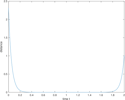
Figure 2. Distance to the stationary solution at each time $t\in[0,T]$, for $\nu=0.5,T=2,N_{T}=200$ and $N_{h}=128$. The distance is computed using the $\ell^{2}$ norm as explained in the text. The turnpike phenomenon is observed as for a long time frame the time-dependent mass approaches the solution of the stationary MFG.

For the multi-grid preconditioner, Table 3 shows the computation times for different discretizations. It can be observed that finer meshes with $128^{3}$ degrees of freedom are solvable within CPU times which outperfom others methods shown in the Appendix and in [14]. Furthermore, the method is robust with respect to different viscosities.

From Table 3 we observe that most of the computational time is used for solving the second proximal operator (the third equality of (4.9)), which does not use a multigrid strategy but which is a pointwise operator (see Proposition $3.1$ of [14]) and thus could be fully paralellizable.

(a) Grid with $64\times 64\times 64$ points.

$\nu$	Total time	Time first prox	Iterations
$0.6$	$116.3$ [s]	$11.50$ [s]	$20$
$0.36$	$120.4$ [s]	$11.40$ [s]	$21$
$0.2$	$119.0$ [s]	$11.26$ [s]	$22$
$0.12$	$129.1$ [s]	$14.11$ [s]	$22$
$0.046$	$225.0$ [s]	$23.28$ [s]	$39$

(b) Grid with $128\times 128\times 128$ points.

$\nu$	Total time	Time first prox	Iterations
$0.6$	$921.1$ [s]	$107.2$ [s]	$20$
$0.36$	$952.3$ [s]	$118.0$ [s]	$21$
$0.2$	$1028.8$ [s]	$127.6$ [s]	$22$
$0.12$	$1036.4$ [s]	$135.5$ [s]	$23$
$0.046$	$1982.2$ [s]	$260.0$ [s]	$42$

Table 3. Time (in seconds) for the convergence of the Chambolle-Pock algorithm, cumulative time of the first proximal operator with the multigrid preconditioner, and number of iterations, for different viscoty values $\nu$ and two types of grids. Here we used $\eta_{1}=\eta_{2}=2,T=1$ and a tolerance between two iterations of the Chambolle-Pock algorithm equal to $10^{-6}$ in normalized $\ell^{2}$-norm.

Unlike the stationary case, low viscosities seem to make the algorithm be slightly slower. However, Table 4 shows that the average number of iterations of BiCGStab stays low regardless of the viscosity. Indeed Table 3 shows that more Chambolle-Pock iterations are needed to converge. The same behavior happens when we use a direct exact solver instead of the multi-grid preconditioned BiCGStab algorithm.

(a) iterations to decrease the residual by a factor $10^{-3}$.

$\nu$	$32\times 32\times 32$	$64\times 64\times 64$	$128\times 128\times 128$
$0.6$	$1.65$	$1.86$	$2.33$
$0.36$	$1.62$	$1.90$	$2.43$
$0.2$	$1.68$	$1.93$	$2.59$
$0.12$	$1.84$	$2.25$	$2.65$
$0.046$	$1.68$	$2.05$	$2.63$

(b) iterations to solve the system with an error of $10^{-8}$.

$\nu$	$32\times 32\times 32$	$64\times 64\times 64$	$128\times 128\times 128$
$0.6$	$3.33$	$3.40$	$3.38$
$0.36$	$3.10$	$3.21$	$3.83$
$0.2$	$3.07$	$3.31$	$4.20$
$0.12$	$3.25$	$3.73$	$4.64$
$0.046$	$2.88$	$3.59$	$4.67$

Table 4. Average number of iterations of the preconditioned BiCGStab with $\eta_{1}=\eta_{2}=2,T=1$ and a tolerance between two iterations of the Chambolle-Pock algorithm equal to $10^{-6}$ in normalized $\ell^{2}$-norm.

Concluding Remarks. In this work we have developed a first-order primal-dual algorithm for the solution of second-order, time-dependent mean field games. The procedure consists of: a variational formulation for the MFG, its discretization via finite differences, the application Chambolle-Pock algorithm to the resulting minimization. While this method has been studied for stationary MFG in [14], its numerical realization for time-dependent MFGs was prohibitive in terms of computing time, as the Chambolle-Pock iteration requires the solution of a large-scale linear system at each iteration. We have overcome this difficulty by studying different preconditioning strategies for the associated linear system. Overall, the multigrid preconditioner with a BiCGStab iteration performs satisfactorily for different discretizations and viscosity values.

Acknowledgments. The third author wants to acknowledge funding within the ANR project MFG ANR-16-CE40-0015-01 operated by the French National Research Agency (ANR).

Most of this work was realized while the fourth author was a postdoctoral fellow at NYU Shanghai and supported by a discretionary research fund.

During the first phase of the project, the fifth author was affiliated to the Unité de Mathématiques Pures et Appliquées (UMPA) UMR CNRS $5669$, of the École Normale Supérieure de Lyon and to the Project-Team Beagle of the Inria Rhône-Alpes. He wishes to acknowledge funding within the framework of the LABEX MILYON (ANR-10-LABX-0070) of the Université de Lyon, within the program ”Investissements d’Avenir” (ANR-11-IDEX-0007). In addition, his participation to this project has been partially supported by the European Research Council (ERC) under the European Union’s Horizon 2020 research and innovation program (grant agreement No. 639638). His participation to this project has also been partially supported by a CEMRACS 2017 scholarship.

The sixth author thanks the support from the PGMO project VarPDEMFG and from the ANR project MFG ANR-16-CE40-0015-01.

Appendix

(a) Unpreconditioned

	16	32	64	128
$5\times 10^{-4}$	18,5	87,6	448	1720
$5\times 10^{-3}$	22,1	98,6	392	1750
$5\times 10^{-2}$	20,7	93,4	607	8240
$0.5$	24,9	113	[X]	[X]

(b) michol

	16	32	64	128
$5\times 10^{-4}$	15,8	77,8	346	1390
$5\times 10^{-3}$	12,4	80,9	325	1244
$5\times 10^{-2}$	5,47	26,3	138	636
$0.5$	3,69	16,5	[X]	[X]

Table 5. Conjugate Gradient computation times (s). (a) Unpreconditioned. (b) Preconditioned with modified incomplete Cholesky factorization. Time discretization: $N_{T}=40$. [X] indicates no convergence.

(a) Unpreconditioned

	8	16	32	64	128
$5\times 10^{-4}$	2.42	14.2	69.0	294	1210
$5\times 10^{-3}$	3.09	16.3	63.9	270	1210
$5\times 10^{-2}$	1.41	12.9	61.3	389	5470
$0.5$	3.41	16.5	98.9	[X]	[X]

(b) michol

	16	32	64	128
$5\times 10^{-4}$	15.7	80.4	412	1890
$5\times 10^{-3}$	12.2	82.2	369	1650
$5\times 10^{-2}$	5.25	27.2	174	894
$0.5$	3.53	18.8	122	2120

Table 6. BiCGStab computation times (s). (a) Unpreconditioned. (b) Preconditioned with modified incomplete Cholesky factorization. Time discretization: $N_{T}=40$. [X] indicates no convergence.

References

- [1] Y. Achdou, F. Camilli, and I. Capuzzo-Dolcetta. Mean field games: numerical methods for the planning problem. SIAM J. Control Optim., 50(1):77–109, 2012.
- [2] Y. Achdou, F. Camilli, and I. Capuzzo-Dolcetta. Mean field games: convergence of a finite difference method. SIAM J. Numer. Anal., 51(5):2585–2612, 2013.
- [3] Y. Achdou and I. Capuzzo-Dolcetta. Mean field games: numerical methods. SIAM J. Numer. Anal., 48(3):1136–1162, 2010.
- [4] Y. Achdou and V. Perez. Iterative strategies for solving linearized discrete mean field games systems. Netw. Heterog. Media, 7(2):197–217, 2012.
- [5] Y. Achdou and A. Porretta. Convergence of a finite difference scheme to weak solutions of the system of partial differential equations arising in mean field games. SIAM J. Numer. Anal., 54(1):161–186, 2016.
- [6] G. Albi, Young-Pil Choi, M. Fornasier, and D. Kalise. Mean-field control hierarchy. Appl. Math. Optim., 76(1):93–175, 2017.
- [7] R. Andreev. Preconditioning the augmented Lagrangian method for instationary mean field games with diffusion. SIAM J. Sci. Comput., 39(6):A2763–A2783, 2017.
- [8] H. H. Bauschke and P.-L. Combettes. Convex analysis and monotone operator theory in Hilbert spaces. CMS Books in Mathematics/Ouvrages de Mathématiques de la SMC. Springer, Cham, second edition, 2017.
- [9] J.-D. Benamou and G. Carlier. Augmented Lagrangian methods for transport optimization, mean field games and degenerate elliptic equations. J. Optim. Theory Appl., 167(1):1–26, 2015.
- [10] A. Bensoussan, J. Frehse, and P. Yam. Mean field games and mean field type control theory. SpringerBriefs in Mathematics. Springer, New York, 2013.
- [11] M. Benzi. Preconditioning techniques for large linear systems: A survey. J. Comput. Phys., 182(2):418–477, nov 2002.
- [12] A. Brandt. Rigorous quantitative analysis of multigrid. I. Constant coefficients two-level cycle with -norm. SIAM J. Numer. Anal., 31(6):1695–1730, 1994.
- [13] L. M. Briceño-Arias and P.-L Combettes. A monotone+ skew splitting model for composite monotone inclusions in duality. SIAM J. Optim., 21(4):1230–1250, 2011.
- [14] L. M. Briceño-Arias, D. Kalise, and F. J. Silva. Proximal methods for stationary mean field games with local couplings. SIAM J. Control Optim., 56(2):801–836, 2018.
- [15] M. Burger, M. Di Francesco, P. A. Markowich, and M. T. Wolfram. Mean field games with nonlinear mobilities in pedestrian dynamics. Discrete Contin. Dyn. Syst. Ser. B, 19(5):1311–1333, 2014.
- [16] P. Cardaliaguet. Notes on Mean Field Games: from P.-L. Lions’ lectures at Collège de France. Lecture Notes given at Tor Vergata, 2010.
- [17] P. Cardaliaguet. Weak solutions for first order mean field games with local coupling. In Analysis and geometry in control theory and its applications, volume 11 of Springer INdAM Ser., pages 111–158. Springer, Cham, 2015.
- [18] P. Cardaliaguet and P. J. Graber. Mean field games systems of first order. ESAIM Control Optim. Calc. Var., 21(3):690–722, 2015.
- [19] P. Cardaliaguet, P. J. Graber, A. Porretta, and D. Tonon. Second order mean field games with degenerate diffusion and local coupling. NoDEA Nonlinear Differential Equations Appl., 22(5):1287–1317, 2015.
- [20] A. Chambolle and T. Pock. A first-order primal-dual algorithm for convex problems with applications to imaging. J. Math. Imaging Vision, 40(1):120–145, 2011.
- [21] G. Chen and M. Teboulle. A proximal-based decomposition method for convex minimization problems. Math. Program., 64:81–101, 1994.
- [22] D Gabay and B Mercier. A dual algorithm for the solution of nonlinear variational problems via finite element approximation. Comput. Math. Appl., 2(1):17–40, 1976.
- [23] R. Glowinski and A. Marrocco. Sur l’approximation, par éléments finis d’ordre un, et la résolution, par pénalisation-dualité, d’une classe de problèmes de Dirichlet non linéaires. Rev. Française Automat. Informat. Recherche Opérationnelle Sér. Rouge Anal. Numér., 9(R-2):41–76, 1975.
- [24] D.-A. Gomes, E. A. Pimentel, and V. Voskanyan. Regularity theory for mean-field game systems. SpringerBriefs in Mathematics. Springer, Cham, 2016.
- [25] D.-A. Gomes and J. Saúde. Mean field games models - a brief survey. Dyn. Games Appl., 4(2):110–154, 2014.
- [26] A. Lachapelle, J. Salomon, and G. Turinici. Computation of mean field equilibria in economics. Math. Models Methods Appl. Sci., 20(4):567–588, 2010.
- [27] J.-M. Lasry and P.-L. Lions. Jeux à champ moyen II. Horizon fini et contrôle optimal. C. R. Math. Acad. Sci. Paris, 343:679–684, 2006.
- [28] J.-M. Lasry and P.-L. Lions. Mean field games. Jpn. J. Math., 2:229–260, 2007.
- [29] A. R. Mészáros and F. J. Silva. A variational approach to second order mean field games with density constraints: the stationary case. J. Math. Pures Appl. (9), 104(6):1135–1159, 2015.
- [30] A. R. Mészáros and F. J. Silva. On the variational formulation of some stationary second order mean field games systems. SIAM J. Mathematical Analysis, 50(1):1255–1277, 2018.
- [31] N. Papadakis, G. Peyré, and E. Oudet. Optimal transport with proximal splitting. SIAM J. Imaging Sci., 7(1):212–238, 2014.
- [32] A. Porretta. Weak solutions to Fokker-Planck equations and mean field games. Arch. Ration. Mech. Anal., 216(1):1–62, 2015.
- [33] A. Porretta and E. Zuazua. Remarks on long time versus steady state optimal control. In Mathematical Paradigms of Climate Science, pages 67–89. Springer, Cham, 2016.
- [34] R. T. Rockafellar. Duality and stability in extremum problems involving convex functions. Pacific J. Math., 21:167–187, 1967.
- [35] U. Trottenberg, C. W. Oosterlee, and A. Schuller. Multigrid. Academic Press, 2000.
- [36] H. Wendland. Numerical Linear Algebra. Cambridge Texts in Applied Mathematics. Cambridge University Press, Cambridge, United Kindgom, first edition, 2017.