Unexpected Phenomenology in Particle-Based Ice Absent in Magnetic Spin Ice

Abstract

While particle-based ices are often considered essentially equivalent to magnet-based spin ices, the two differ essentially in frustration and energetics. We show that at equilibrium particle-based ices correspond exactly to spin ices coupled to a background field. In trivial geometries, such a field has no effect, and the two systems are indeed thermodynamically equivalent. In other cases, however, the field controls a richer phenomenology, absent in magnetic ices, and still largely unexplored: ice rule fragility, topological charge transfer, radial polarization, decimation induced disorder, and glassiness.

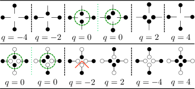
Introduction. The ice rule Bernal and Fowler (1933) has had an impactful history. Pauling employed it to explain Pauling (1935) the zero point entropy of water ice Giauque and Stout (1936) as a consequence of the degeneracy in allocating two protons close to, and two away from, each oxygen atom sitting in any of the tetrahedron-based crystal structures of ice. However, the concept is more general. Consider binary spins placed along the edges of a graph, impinging in its vertices (Fig. 1). The topological charge of a vertex of coordination $z$ is the difference between the $n$ spins pointing in and the $z-n$ pointing out, or $q_{n}=2n-z$ (Fig 1). Then, an ice-manifold is the degenerate set of spin configurations that minimizes $|q|$ locally. If $z$ is even, the minimal $|q|$ is zero (for $z=4$, we recover the original ice rule, 2-in/2-out, of water ice and rare earth titanates magnets Ramirez et al. (1999)). If $z$ is odd, ice rule vertices have charges $q=\pm 1$ and the ice-manifold is a neutral plasma of topological charges Möller and Moessner (2009); Chern et al. (2011); Rougemaille et al. (2011a); Zhang et al. (2013); Anghinolfi et al. (2015).

As Ice manifolds can typically host unusual phases Nisoli et al. (2017), they have invited the design of a new class of artificial, frustrated magnetic nano-materials, called “artificial spin ices” (SI). These are arrays of interacting, single-domain, shape-anisotropic, magnetic nano-islands whose magnetizations are described by binary spin and obey the ice rule (Fig. 1a,b) Wang et al. (2006); Nisoli et al. (2013). Their exotic behaviors are often not found in natural magnets Morrison et al. (2013) and can be designed to study memory effects Gilbert et al. (2015), effective thermodynamics in driven systems Nisoli et al. (2010), magnetic charges and monopoles Mengotti et al. (2010); Rougemaille et al. (2011b); Ladak et al. (2011); Zhang et al. (2013), anomalous hall effects Branford et al. (2012); Le et al. (2017), often with real time, real space characterization Farhan et al. (2013); Kapaklis et al. (2014); Porro et al. (2013); Gilbert et al. (2016a, b).

“Particle ices” (PI) are another artificial implementation of an ice manifold Libál et al. (2006, 2009); Reichhardt et al. (2012); Libal et al. (2017); Libál et al. (2012, 2017). Mutually repulsive particles are trapped, one particle per trap, with preferential occupation at its extremes (Fig. 1c,d). Traps are arranged along the edges of a lattice whose geometry determines the collective behavior. They have been studied numerically Libál et al. (2006, 2009); Reichhardt et al. (2012) and realized experimentally using magnetic colloids gravitationally trapped in microgrooves Ortiz-Ambriz and Tierno (2016); Loehr et al. (2016) but also in flux quanta pinned to nano-patterned superconductors Latimer et al. (2013); Trastoy et al. (2014); Ge et al. (2017). As PI was also found to obey the ice rule, at least in the square and hexagonal geometry, ideas and results have been exchanged among PI and SI, often considered as essentially equivalent systems. That assumption is incorrect.

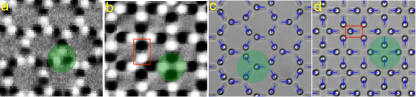
Figure 1: Magnetic force microscopy of hexagonal (a) and square (b) SI show the constitutive degrees of freedom (red rectangles) as dumbbells of positive (white) and negative (black) magnetic charge (from Nisoli et al. (2010)). Optical microscopy of hexagonal (c) and square (d) SI, where the blue arrows denote the equivalent spins (from Ortiz-Ambriz and Tierno (2016)). Green disks show ice rule obeying vertices.

Indeed, despite similarities, the two systems differ essentially in energetics and frustration. While local energetics promotes the ice rule in SI, it opposes it in PI. The energy of a SI vertex is typically proportional to the square of its topological charge, $E\propto q_{n}^{2}$, thus favoring the ice rule. For PI, it is instead $E\propto n(n-1)$, thus favoring large negative charges which violate the ice-rule (Figs. 2, 3). In PI the ice-manifold emerges as a collective energetic compromise in the thermodynamic limit Nisoli (2014); Libal and et al (2017) from the constraint that the total charge must be zero. It is thus locally unstable and fragile. It is a “thin ice”.

We provide here a unifying framework for the complex phenomenology of similarities and differences among the two classes of materials: PI at equilibrium can be mapped directly into a SI coupled to a geometry-dependent background field. In trivial geometries the field is zero and the two ices are equivalent. In non-trivial ones, however, it mediates the breakdown of the ice rule, leading to an entirely new phenomenology, still largely unexplored. Without pretenses of exhaustiveness we propose some implications of this mapping to suggest exotic, novel behaviors which invite further experimental exploration.

1—Isomorphism. In PI, particles in positions $\{{\bf y}\}$ repel with interaction $\phi(r)$. Clearly, their total energy ${\cal H}=\sum_{{\bf y}\neq{\bf y^{\prime}}}\phi\left(|{\bf y}-{\bf y^{\prime}}|\right)$ does not appear very conducive to SI physics.

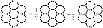
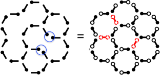
Figure 2: Top: Schematic illustration of Eq. (1) where an hexagonal PI (here in a random configuration) is decomposed into a SI, with dipolar degrees of freedom, plus a background of positively saturated traps. The energy of the PI (middle) and SI (bottom) vertices, listed in increasing order (from left to right, separated by dotted vertical lines) differ essentially. PI promotes vertices of large negative charge, violating $\mathbb{Z}_{2}$ symmetry. SI promotes vertices of low absolute topological charge (ice rule, circled in green).

Yet, at equilibrium the position of the particle in a trap is a binary variable, represented by — or — (Fig 1c,d). We can map PI into SI by ascribing a positive charge to our particles, and introducing virtual negative charges , which repel (resp. attract) other negative (positive) charges. Then, the energy does not change if we fractionalize each trap as a trap doubly occupied by positive charges (or positive dumbbell $\operatorname{\leavevmode\hbox to6.4pt{\vbox to6.4pt{\pgfpicture\makeatletter\hbox{\hskip 3.2pt\lower-3.2pt\hbox to0.0pt{\pgfsys@beginscope\pgfsys@invoke{ }\definecolor{pgfstrokecolor}{rgb}{0,0,0}\pgfsys@color@rgb@stroke{0}{0}{0}\pgfsys@invoke{ }\pgfsys@color@rgb@fill{0}{0}{0}\pgfsys@invoke{ }\pgfsys@setlinewidth{0.4pt}\pgfsys@invoke{ }\nullfont\hbox to0.0pt{\pgfsys@beginscope\pgfsys@invoke{ }{}{{}}{}{{{}} {}{}{}{}{}{}{}{} }\pgfsys@beginscope\pgfsys@invoke{ }\color[rgb]{0,0,0}\definecolor[named]{pgfstrokecolor}{rgb}{0,0,0}\pgfsys@color@gray@stroke{0}\pgfsys@invoke{ }\pgfsys@color@gray@fill{0}\pgfsys@invoke{ }\definecolor[named]{pgffillcolor}{rgb}{0,0,0}\definecolor[named]{pgffillcolor}{rgb}{0,0,0}\pgfsys@color@gray@fill{0}\pgfsys@invoke{ }{}\pgfsys@moveto{0.0pt}{0.0pt}\pgfsys@moveto{3.0pt}{0.0pt}\pgfsys@curveto{3.0pt}{1.65688pt}{1.65688pt}{3.0pt}{0.0pt}{3.0pt}\pgfsys@curveto{-1.65688pt}{3.0pt}{-3.0pt}{1.65688pt}{-3.0pt}{0.0pt}\pgfsys@curveto{-3.0pt}{-1.65688pt}{-1.65688pt}{-3.0pt}{0.0pt}{-3.0pt}\pgfsys@curveto{1.65688pt}{-3.0pt}{3.0pt}{-1.65688pt}{3.0pt}{0.0pt}\pgfsys@closepath\pgfsys@moveto{0.0pt}{0.0pt}\pgfsys@fillstroke\pgfsys@invoke{ } \pgfsys@invoke{\lxSVG@closescope }\pgfsys@endscope \pgfsys@invoke{\lxSVG@closescope }\pgfsys@endscope{}{}{}\hss}\pgfsys@discardpath\pgfsys@invoke{\lxSVG@closescope }\pgfsys@endscope\hss}}\lxSVG@closescope\endpgfpicture}}---\leavevmode\hbox to6.4pt{\vbox to6.4pt{\pgfpicture\makeatletter\hbox{\hskip 3.2pt\lower-3.2pt\hbox to0.0pt{\pgfsys@beginscope\pgfsys@invoke{ }\definecolor{pgfstrokecolor}{rgb}{0,0,0}\pgfsys@color@rgb@stroke{0}{0}{0}\pgfsys@invoke{ }\pgfsys@color@rgb@fill{0}{0}{0}\pgfsys@invoke{ }\pgfsys@setlinewidth{0.4pt}\pgfsys@invoke{ }\nullfont\hbox to0.0pt{\pgfsys@beginscope\pgfsys@invoke{ }{}{{}}{}{{{}} {}{}{}{}{}{}{}{} }\pgfsys@beginscope\pgfsys@invoke{ }\color[rgb]{0,0,0}\definecolor[named]{pgfstrokecolor}{rgb}{0,0,0}\pgfsys@color@gray@stroke{0}\pgfsys@invoke{ }\pgfsys@color@gray@fill{0}\pgfsys@invoke{ }\definecolor[named]{pgffillcolor}{rgb}{0,0,0}\definecolor[named]{pgffillcolor}{rgb}{0,0,0}\pgfsys@color@gray@fill{0}\pgfsys@invoke{ }{}\pgfsys@moveto{0.0pt}{0.0pt}\pgfsys@moveto{3.0pt}{0.0pt}\pgfsys@curveto{3.0pt}{1.65688pt}{1.65688pt}{3.0pt}{0.0pt}{3.0pt}\pgfsys@curveto{-1.65688pt}{3.0pt}{-3.0pt}{1.65688pt}{-3.0pt}{0.0pt}\pgfsys@curveto{-3.0pt}{-1.65688pt}{-1.65688pt}{-3.0pt}{0.0pt}{-3.0pt}\pgfsys@curveto{1.65688pt}{-3.0pt}{3.0pt}{-1.65688pt}{3.0pt}{0.0pt}\pgfsys@closepath\pgfsys@moveto{0.0pt}{0.0pt}\pgfsys@fillstroke\pgfsys@invoke{ } \pgfsys@invoke{\lxSVG@closescope }\pgfsys@endscope \pgfsys@invoke{\lxSVG@closescope }\pgfsys@endscope{}{}{}\hss}\pgfsys@discardpath\pgfsys@invoke{\lxSVG@closescope }\pgfsys@endscope\hss}}\lxSVG@closescope\endpgfpicture}}}$), plus a dipole of negative and positive charges $\vec{\sigma}=\operatorname{\leavevmode\hbox to6.4pt{\vbox to6.4pt{\pgfpicture\makeatletter\hbox{\hskip 3.2pt\lower-3.2pt\hbox to0.0pt{\pgfsys@beginscope\pgfsys@invoke{ }\definecolor{pgfstrokecolor}{rgb}{0,0,0}\pgfsys@color@rgb@stroke{0}{0}{0}\pgfsys@invoke{ }\pgfsys@color@rgb@fill{0}{0}{0}\pgfsys@invoke{ }\pgfsys@setlinewidth{0.4pt}\pgfsys@invoke{ }\nullfont\hbox to0.0pt{\pgfsys@beginscope\pgfsys@invoke{ }{}{{}}{}{{{}} {}{}{}{}{}{}{}{} }\pgfsys@beginscope\pgfsys@invoke{ }\color[rgb]{0,0,0}\definecolor[named]{pgfstrokecolor}{rgb}{0,0,0}\pgfsys@color@gray@stroke{0}\pgfsys@invoke{ }\pgfsys@color@gray@fill{0}\pgfsys@invoke{ }\definecolor[named]{pgffillcolor}{rgb}{0,0,0}\definecolor[named]{pgffillcolor}{rgb}{1,1,1}\pgfsys@color@gray@fill{1}\pgfsys@invoke{ }{}\pgfsys@moveto{0.0pt}{0.0pt}\pgfsys@moveto{3.0pt}{0.0pt}\pgfsys@curveto{3.0pt}{1.65688pt}{1.65688pt}{3.0pt}{0.0pt}{3.0pt}\pgfsys@curveto{-1.65688pt}{3.0pt}{-3.0pt}{1.65688pt}{-3.0pt}{0.0pt}\pgfsys@curveto{-3.0pt}{-1.65688pt}{-1.65688pt}{-3.0pt}{0.0pt}{-3.0pt}\pgfsys@curveto{1.65688pt}{-3.0pt}{3.0pt}{-1.65688pt}{3.0pt}{0.0pt}\pgfsys@closepath\pgfsys@moveto{0.0pt}{0.0pt}\pgfsys@fillstroke\pgfsys@invoke{ } \pgfsys@invoke{\lxSVG@closescope }\pgfsys@endscope \pgfsys@invoke{\lxSVG@closescope }\pgfsys@endscope{}{}{}\hss}\pgfsys@discardpath\pgfsys@invoke{\lxSVG@closescope }\pgfsys@endscope\hss}}\lxSVG@closescope\endpgfpicture}}---\leavevmode\hbox to6.4pt{\vbox to6.4pt{\pgfpicture\makeatletter\hbox{\hskip 3.2pt\lower-3.2pt\hbox to0.0pt{\pgfsys@beginscope\pgfsys@invoke{ }\definecolor{pgfstrokecolor}{rgb}{0,0,0}\pgfsys@color@rgb@stroke{0}{0}{0}\pgfsys@invoke{ }\pgfsys@color@rgb@fill{0}{0}{0}\pgfsys@invoke{ }\pgfsys@setlinewidth{0.4pt}\pgfsys@invoke{ }\nullfont\hbox to0.0pt{\pgfsys@beginscope\pgfsys@invoke{ }{}{{}}{}{{{}} {}{}{}{}{}{}{}{} }\pgfsys@beginscope\pgfsys@invoke{ }\color[rgb]{0,0,0}\definecolor[named]{pgfstrokecolor}{rgb}{0,0,0}\pgfsys@color@gray@stroke{0}\pgfsys@invoke{ }\pgfsys@color@gray@fill{0}\pgfsys@invoke{ }\definecolor[named]{pgffillcolor}{rgb}{0,0,0}\definecolor[named]{pgffillcolor}{rgb}{0,0,0}\pgfsys@color@gray@fill{0}\pgfsys@invoke{ }{}\pgfsys@moveto{0.0pt}{0.0pt}\pgfsys@moveto{3.0pt}{0.0pt}\pgfsys@curveto{3.0pt}{1.65688pt}{1.65688pt}{3.0pt}{0.0pt}{3.0pt}\pgfsys@curveto{-1.65688pt}{3.0pt}{-3.0pt}{1.65688pt}{-3.0pt}{0.0pt}\pgfsys@curveto{-3.0pt}{-1.65688pt}{-1.65688pt}{-3.0pt}{0.0pt}{-3.0pt}\pgfsys@curveto{1.65688pt}{-3.0pt}{3.0pt}{-1.65688pt}{3.0pt}{0.0pt}\pgfsys@closepath\pgfsys@moveto{0.0pt}{0.0pt}\pgfsys@fillstroke\pgfsys@invoke{ } \pgfsys@invoke{\lxSVG@closescope }\pgfsys@endscope \pgfsys@invoke{\lxSVG@closescope }\pgfsys@endscope{}{}{}\hss}\pgfsys@discardpath\pgfsys@invoke{\lxSVG@closescope }\pgfsys@endscope\hss}}\lxSVG@closescope\endpgfpicture}}}$:

$$\operatorname{-----\leavevmode\hbox to6.4pt{\vbox to6.4pt{\pgfpicture\makeatletter\hbox{\hskip 3.2pt\lower-3.2pt\hbox to0.0pt{\pgfsys@beginscope\pgfsys@invoke{ }\definecolor{pgfstrokecolor}{rgb}{0,0,0}\pgfsys@color@rgb@stroke{0}{0}{0}\pgfsys@invoke{ }\pgfsys@color@rgb@fill{0}{0}{0}\pgfsys@invoke{ }\pgfsys@setlinewidth{0.4pt}\pgfsys@invoke{ }\nullfont\hbox to0.0pt{\pgfsys@beginscope\pgfsys@invoke{ }{}{{}}{}{{{}} {}{}{}{}{}{}{}{} }\pgfsys@beginscope\pgfsys@invoke{ }\color[rgb]{0,0,0}\definecolor[named]{pgfstrokecolor}{rgb}{0,0,0}\pgfsys@color@gray@stroke{0}\pgfsys@invoke{ }\pgfsys@color@gray@fill{0}\pgfsys@invoke{ }\definecolor[named]{pgffillcolor}{rgb}{0,0,0}\definecolor[named]{pgffillcolor}{rgb}{0,0,0}\pgfsys@color@gray@fill{0}\pgfsys@invoke{ }{}\pgfsys@moveto{0.0pt}{0.0pt}\pgfsys@moveto{3.0pt}{0.0pt}\pgfsys@curveto{3.0pt}{1.65688pt}{1.65688pt}{3.0pt}{0.0pt}{3.0pt}\pgfsys@curveto{-1.65688pt}{3.0pt}{-3.0pt}{1.65688pt}{-3.0pt}{0.0pt}\pgfsys@curveto{-3.0pt}{-1.65688pt}{-1.65688pt}{-3.0pt}{0.0pt}{-3.0pt}\pgfsys@curveto{1.65688pt}{-3.0pt}{3.0pt}{-1.65688pt}{3.0pt}{0.0pt}\pgfsys@closepath\pgfsys@moveto{0.0pt}{0.0pt}\pgfsys@fillstroke\pgfsys@invoke{ } \pgfsys@invoke{\lxSVG@closescope }\pgfsys@endscope \pgfsys@invoke{\lxSVG@closescope }\pgfsys@endscope{}{}{}\hss}\pgfsys@discardpath\pgfsys@invoke{\lxSVG@closescope }\pgfsys@endscope\hss}}\lxSVG@closescope\endpgfpicture}}}=\frac{1}{2}\operatorname{\leavevmode\hbox to6.4pt{\vbox to6.4pt{\pgfpicture\makeatletter\hbox{\hskip 3.2pt\lower-3.2pt\hbox to0.0pt{\pgfsys@beginscope\pgfsys@invoke{ }\definecolor{pgfstrokecolor}{rgb}{0,0,0}\pgfsys@color@rgb@stroke{0}{0}{0}\pgfsys@invoke{ }\pgfsys@color@rgb@fill{0}{0}{0}\pgfsys@invoke{ }\pgfsys@setlinewidth{0.4pt}\pgfsys@invoke{ }\nullfont\hbox to0.0pt{\pgfsys@beginscope\pgfsys@invoke{ }{}{{}}{}{{{}} {}{}{}{}{}{}{}{} }\pgfsys@beginscope\pgfsys@invoke{ }\color[rgb]{0,0,0}\definecolor[named]{pgfstrokecolor}{rgb}{0,0,0}\pgfsys@color@gray@stroke{0}\pgfsys@invoke{ }\pgfsys@color@gray@fill{0}\pgfsys@invoke{ }\definecolor[named]{pgffillcolor}{rgb}{0,0,0}\definecolor[named]{pgffillcolor}{rgb}{0,0,0}\pgfsys@color@gray@fill{0}\pgfsys@invoke{ }{}\pgfsys@moveto{0.0pt}{0.0pt}\pgfsys@moveto{3.0pt}{0.0pt}\pgfsys@curveto{3.0pt}{1.65688pt}{1.65688pt}{3.0pt}{0.0pt}{3.0pt}\pgfsys@curveto{-1.65688pt}{3.0pt}{-3.0pt}{1.65688pt}{-3.0pt}{0.0pt}\pgfsys@curveto{-3.0pt}{-1.65688pt}{-1.65688pt}{-3.0pt}{0.0pt}{-3.0pt}\pgfsys@curveto{1.65688pt}{-3.0pt}{3.0pt}{-1.65688pt}{3.0pt}{0.0pt}\pgfsys@closepath\pgfsys@moveto{0.0pt}{0.0pt}\pgfsys@fillstroke\pgfsys@invoke{ } \pgfsys@invoke{\lxSVG@closescope }\pgfsys@endscope \pgfsys@invoke{\lxSVG@closescope }\pgfsys@endscope{}{}{}\hss}\pgfsys@discardpath\pgfsys@invoke{\lxSVG@closescope }\pgfsys@endscope\hss}}\lxSVG@closescope\endpgfpicture}}---\leavevmode\hbox to6.4pt{\vbox to6.4pt{\pgfpicture\makeatletter\hbox{\hskip 3.2pt\lower-3.2pt\hbox to0.0pt{\pgfsys@beginscope\pgfsys@invoke{ }\definecolor{pgfstrokecolor}{rgb}{0,0,0}\pgfsys@color@rgb@stroke{0}{0}{0}\pgfsys@invoke{ }\pgfsys@color@rgb@fill{0}{0}{0}\pgfsys@invoke{ }\pgfsys@setlinewidth{0.4pt}\pgfsys@invoke{ }\nullfont\hbox to0.0pt{\pgfsys@beginscope\pgfsys@invoke{ }{}{{}}{}{{{}} {}{}{}{}{}{}{}{} }\pgfsys@beginscope\pgfsys@invoke{ }\color[rgb]{0,0,0}\definecolor[named]{pgfstrokecolor}{rgb}{0,0,0}\pgfsys@color@gray@stroke{0}\pgfsys@invoke{ }\pgfsys@color@gray@fill{0}\pgfsys@invoke{ }\definecolor[named]{pgffillcolor}{rgb}{0,0,0}\definecolor[named]{pgffillcolor}{rgb}{0,0,0}\pgfsys@color@gray@fill{0}\pgfsys@invoke{ }{}\pgfsys@moveto{0.0pt}{0.0pt}\pgfsys@moveto{3.0pt}{0.0pt}\pgfsys@curveto{3.0pt}{1.65688pt}{1.65688pt}{3.0pt}{0.0pt}{3.0pt}\pgfsys@curveto{-1.65688pt}{3.0pt}{-3.0pt}{1.65688pt}{-3.0pt}{0.0pt}\pgfsys@curveto{-3.0pt}{-1.65688pt}{-1.65688pt}{-3.0pt}{0.0pt}{-3.0pt}\pgfsys@curveto{1.65688pt}{-3.0pt}{3.0pt}{-1.65688pt}{3.0pt}{0.0pt}\pgfsys@closepath\pgfsys@moveto{0.0pt}{0.0pt}\pgfsys@fillstroke\pgfsys@invoke{ } \pgfsys@invoke{\lxSVG@closescope }\pgfsys@endscope \pgfsys@invoke{\lxSVG@closescope }\pgfsys@endscope{}{}{}\hss}\pgfsys@discardpath\pgfsys@invoke{\lxSVG@closescope }\pgfsys@endscope\hss}}\lxSVG@closescope\endpgfpicture}}}+\frac{1}{2}\operatorname{\leavevmode\hbox to6.4pt{\vbox to6.4pt{\pgfpicture\makeatletter\hbox{\hskip 3.2pt\lower-3.2pt\hbox to0.0pt{\pgfsys@beginscope\pgfsys@invoke{ }\definecolor{pgfstrokecolor}{rgb}{0,0,0}\pgfsys@color@rgb@stroke{0}{0}{0}\pgfsys@invoke{ }\pgfsys@color@rgb@fill{0}{0}{0}\pgfsys@invoke{ }\pgfsys@setlinewidth{0.4pt}\pgfsys@invoke{ }\nullfont\hbox to0.0pt{\pgfsys@beginscope\pgfsys@invoke{ }{}{{}}{}{{{}} {}{}{}{}{}{}{}{} }\pgfsys@beginscope\pgfsys@invoke{ }\color[rgb]{0,0,0}\definecolor[named]{pgfstrokecolor}{rgb}{0,0,0}\pgfsys@color@gray@stroke{0}\pgfsys@invoke{ }\pgfsys@color@gray@fill{0}\pgfsys@invoke{ }\definecolor[named]{pgffillcolor}{rgb}{0,0,0}\definecolor[named]{pgffillcolor}{rgb}{1,1,1}\pgfsys@color@gray@fill{1}\pgfsys@invoke{ }{}\pgfsys@moveto{0.0pt}{0.0pt}\pgfsys@moveto{3.0pt}{0.0pt}\pgfsys@curveto{3.0pt}{1.65688pt}{1.65688pt}{3.0pt}{0.0pt}{3.0pt}\pgfsys@curveto{-1.65688pt}{3.0pt}{-3.0pt}{1.65688pt}{-3.0pt}{0.0pt}\pgfsys@curveto{-3.0pt}{-1.65688pt}{-1.65688pt}{-3.0pt}{0.0pt}{-3.0pt}\pgfsys@curveto{1.65688pt}{-3.0pt}{3.0pt}{-1.65688pt}{3.0pt}{0.0pt}\pgfsys@closepath\pgfsys@moveto{0.0pt}{0.0pt}\pgfsys@fillstroke\pgfsys@invoke{ } \pgfsys@invoke{\lxSVG@closescope }\pgfsys@endscope \pgfsys@invoke{\lxSVG@closescope }\pgfsys@endscope{}{}{}\hss}\pgfsys@discardpath\pgfsys@invoke{\lxSVG@closescope }\pgfsys@endscope\hss}}\lxSVG@closescope\endpgfpicture}}---\leavevmode\hbox to6.4pt{\vbox to6.4pt{\pgfpicture\makeatletter\hbox{\hskip 3.2pt\lower-3.2pt\hbox to0.0pt{\pgfsys@beginscope\pgfsys@invoke{ }\definecolor{pgfstrokecolor}{rgb}{0,0,0}\pgfsys@color@rgb@stroke{0}{0}{0}\pgfsys@invoke{ }\pgfsys@color@rgb@fill{0}{0}{0}\pgfsys@invoke{ }\pgfsys@setlinewidth{0.4pt}\pgfsys@invoke{ }\nullfont\hbox to0.0pt{\pgfsys@beginscope\pgfsys@invoke{ }{}{{}}{}{{{}} {}{}{}{}{}{}{}{} }\pgfsys@beginscope\pgfsys@invoke{ }\color[rgb]{0,0,0}\definecolor[named]{pgfstrokecolor}{rgb}{0,0,0}\pgfsys@color@gray@stroke{0}\pgfsys@invoke{ }\pgfsys@color@gray@fill{0}\pgfsys@invoke{ }\definecolor[named]{pgffillcolor}{rgb}{0,0,0}\definecolor[named]{pgffillcolor}{rgb}{0,0,0}\pgfsys@color@gray@fill{0}\pgfsys@invoke{ }{}\pgfsys@moveto{0.0pt}{0.0pt}\pgfsys@moveto{3.0pt}{0.0pt}\pgfsys@curveto{3.0pt}{1.65688pt}{1.65688pt}{3.0pt}{0.0pt}{3.0pt}\pgfsys@curveto{-1.65688pt}{3.0pt}{-3.0pt}{1.65688pt}{-3.0pt}{0.0pt}\pgfsys@curveto{-3.0pt}{-1.65688pt}{-1.65688pt}{-3.0pt}{0.0pt}{-3.0pt}\pgfsys@curveto{1.65688pt}{-3.0pt}{3.0pt}{-1.65688pt}{3.0pt}{0.0pt}\pgfsys@closepath\pgfsys@moveto{0.0pt}{0.0pt}\pgfsys@fillstroke\pgfsys@invoke{ } \pgfsys@invoke{\lxSVG@closescope }\pgfsys@endscope \pgfsys@invoke{\lxSVG@closescope }\pgfsys@endscope{}{}{}\hss}\pgfsys@discardpath\pgfsys@invoke{\lxSVG@closescope }\pgfsys@endscope\hss}}\lxSVG@closescope\endpgfpicture}}}.$$ (1)

Then the energy can be rewritten as

$${\cal H}=\sum_{{\bf x}\neq{\bf x}^{\prime}}V\left(\vec{\sigma}_{\bf x},\vec{\sigma}_{\bf x^{\prime}}\right)+\sum_{{\bf x}}W\left(\vec{\sigma}_{\bf x}\right)$$ (2)

(up to an irrelevant constant the self-energy of the saturated traps). The first term represent the SI part of the hamiltonian: $V\left(\vec{\sigma}_{\bf x},\vec{\sigma}_{\bf x^{\prime}}\right)$ is the interaction between the dipolar spins $\vec{\sigma}_{\bf x}$ on the edges ${\bf x}$, and it can in general be reconstructed from $\phi$. The second term is the interaction between dipoles and positive dumbbells: $W\left(\vec{\sigma}_{\bf x}\right)=[\psi\left({\bf x}+\vec{\sigma}_{\bf x}/2\right)-\psi\left({\bf x-}\vec{\sigma}_{\bf x}/2\right)]/2,$ with $\psi({\bf x})=\sum_{{\bf y}_{\bullet}\neq{\bf x}}\phi({\bf x}-{\bf y}_{\bullet})$, where ${\bf y}_{\bullet}$ runs over all the allowed particle positions in all the dumbbells $\operatorname{\leavevmode\hbox to6.4pt{\vbox to6.4pt{\pgfpicture\makeatletter\hbox{\hskip 3.2pt\lower-3.2pt\hbox to0.0pt{\pgfsys@beginscope\pgfsys@invoke{ }\definecolor{pgfstrokecolor}{rgb}{0,0,0}\pgfsys@color@rgb@stroke{0}{0}{0}\pgfsys@invoke{ }\pgfsys@color@rgb@fill{0}{0}{0}\pgfsys@invoke{ }\pgfsys@setlinewidth{0.4pt}\pgfsys@invoke{ }\nullfont\hbox to0.0pt{\pgfsys@beginscope\pgfsys@invoke{ }{}{{}}{}{{{}} {}{}{}{}{}{}{}{} }\pgfsys@beginscope\pgfsys@invoke{ }\color[rgb]{0,0,0}\definecolor[named]{pgfstrokecolor}{rgb}{0,0,0}\pgfsys@color@gray@stroke{0}\pgfsys@invoke{ }\pgfsys@color@gray@fill{0}\pgfsys@invoke{ }\definecolor[named]{pgffillcolor}{rgb}{0,0,0}\definecolor[named]{pgffillcolor}{rgb}{0,0,0}\pgfsys@color@gray@fill{0}\pgfsys@invoke{ }{}\pgfsys@moveto{0.0pt}{0.0pt}\pgfsys@moveto{3.0pt}{0.0pt}\pgfsys@curveto{3.0pt}{1.65688pt}{1.65688pt}{3.0pt}{0.0pt}{3.0pt}\pgfsys@curveto{-1.65688pt}{3.0pt}{-3.0pt}{1.65688pt}{-3.0pt}{0.0pt}\pgfsys@curveto{-3.0pt}{-1.65688pt}{-1.65688pt}{-3.0pt}{0.0pt}{-3.0pt}\pgfsys@curveto{1.65688pt}{-3.0pt}{3.0pt}{-1.65688pt}{3.0pt}{0.0pt}\pgfsys@closepath\pgfsys@moveto{0.0pt}{0.0pt}\pgfsys@fillstroke\pgfsys@invoke{ } \pgfsys@invoke{\lxSVG@closescope }\pgfsys@endscope \pgfsys@invoke{\lxSVG@closescope }\pgfsys@endscope{}{}{}\hss}\pgfsys@discardpath\pgfsys@invoke{\lxSVG@closescope }\pgfsys@endscope\hss}}\lxSVG@closescope\endpgfpicture}}---\leavevmode\hbox to6.4pt{\vbox to6.4pt{\pgfpicture\makeatletter\hbox{\hskip 3.2pt\lower-3.2pt\hbox to0.0pt{\pgfsys@beginscope\pgfsys@invoke{ }\definecolor{pgfstrokecolor}{rgb}{0,0,0}\pgfsys@color@rgb@stroke{0}{0}{0}\pgfsys@invoke{ }\pgfsys@color@rgb@fill{0}{0}{0}\pgfsys@invoke{ }\pgfsys@setlinewidth{0.4pt}\pgfsys@invoke{ }\nullfont\hbox to0.0pt{\pgfsys@beginscope\pgfsys@invoke{ }{}{{}}{}{{{}} {}{}{}{}{}{}{}{} }\pgfsys@beginscope\pgfsys@invoke{ }\color[rgb]{0,0,0}\definecolor[named]{pgfstrokecolor}{rgb}{0,0,0}\pgfsys@color@gray@stroke{0}\pgfsys@invoke{ }\pgfsys@color@gray@fill{0}\pgfsys@invoke{ }\definecolor[named]{pgffillcolor}{rgb}{0,0,0}\definecolor[named]{pgffillcolor}{rgb}{0,0,0}\pgfsys@color@gray@fill{0}\pgfsys@invoke{ }{}\pgfsys@moveto{0.0pt}{0.0pt}\pgfsys@moveto{3.0pt}{0.0pt}\pgfsys@curveto{3.0pt}{1.65688pt}{1.65688pt}{3.0pt}{0.0pt}{3.0pt}\pgfsys@curveto{-1.65688pt}{3.0pt}{-3.0pt}{1.65688pt}{-3.0pt}{0.0pt}\pgfsys@curveto{-3.0pt}{-1.65688pt}{-1.65688pt}{-3.0pt}{0.0pt}{-3.0pt}\pgfsys@curveto{1.65688pt}{-3.0pt}{3.0pt}{-1.65688pt}{3.0pt}{0.0pt}\pgfsys@closepath\pgfsys@moveto{0.0pt}{0.0pt}\pgfsys@fillstroke\pgfsys@invoke{ } \pgfsys@invoke{\lxSVG@closescope }\pgfsys@endscope \pgfsys@invoke{\lxSVG@closescope }\pgfsys@endscope{}{}{}\hss}\pgfsys@discardpath\pgfsys@invoke{\lxSVG@closescope }\pgfsys@endscope\hss}}\lxSVG@closescope\endpgfpicture}}}$.

Thus a PI is a SI under the field $\psi$ generated by the virtual positive dumbbells. We will often adopt a nearest neighbor vertex model Baxter (1982); Lieb (1967) approximation and consider the “energy of a vertex”, i.e. the interaction energies of all the spins impinging in said vertex. Figures 2, 3 show the different energy hierarchies for hexagonal and square geometries in the two pictures, where the SI picture recovers a $\mathbb{Z}_{2}$ symmetry absent in the PI picture.

Figure 3: Same as in Fig. 2, but for the square lattice. Here, however, the degeneracy of the ice-rule vertices ($q=0$) is lifted by a difference in interaction strength between perpendicular and collinear traps or dumbbells (green dotted lines), and polarized vertices have higher energy (middle: forth from left; bottom: second from left). The red $\wedge$ connects two plaquettes where the head-to-toe rule is broken by a monopole (see Fig. 5).

We call a geometry trivially-equivalent if the second term in (2) is a constant: then the the PI becomes a SI. From symmetry considerations, ices whose vertices are the nodes of an infinite Bravais lattice are trivially-equivalent, explaining why the hexagonal and square PI follow the ice rule Libál et al. (2006, 2009).

2—Ice rule and inner phases. SI often exhibits layered phases. E.g., Kagome SI enters a charge-ordered/spin-disordered phase within its ice manifold, and then a long-range ordered, demagnetized phase within its charge-ordered phase Möller and Moessner (2009); Rougemaille et al. (2011a); Chern et al. (2013); Anghinolfi et al. (2015); Zhang et al. (2013). A dipolar expansion of (2)

$${\cal H} \simeq\frac{k}{2}\sum_{v}q^{2}_{v}+\frac{1}{2}\sum_{\langle v,v^{\prime}\rangle}q_{v}q_{v^{\prime}}\phi(r_{v,v^{\prime}})$$

$$+\frac{1}{2}\sum_{{\bf x^{\prime}}\notin\partial{\bf x}}{\sigma}^{i}_{\bf x}J_{ij}\left({\bf x}-{\bf x^{\prime}}\right){\sigma}^{j}_{\bf x^{\prime}}-\sum_{\bf x}\vec{\sigma}_{\bf x}\cdot\vec{E}({\bf x})$$ (3)

shows that PI also admits inner phases. The first term imposes the ice rule from the interaction among dipoles within a vertex ($q_{v}$ is the charge of the vertex $v$, and $k>0$ depends on $\psi$) and implies a crossover to an ice-manifold Libál et al. (2006, 2009). The second term is an interaction between charged vertices and implies charge order at lower temperatures, as was recently seen numerically for PI with repulsion $\phi=x^{-3}$ Libal et al. (2017). The third term is a generalized dipolar interaction among further neighboring spins ($\partial{\bf x}$ is the neighborhood of ${\bf x}$) whose form depends on $\phi$. For instance, for $\phi\propto r^{-\alpha}$ we have immediately

$$J_{ij}({\bf r})\propto\left[\delta_{ij}-(\alpha+2)r_{i}r_{j}\right]{r^{-\alpha-2}},$$ (4)

which reduces to the familiar dipolar interaction for $\alpha=1$. Instead, $\alpha>1$ in (4) strengthens the ferromagnetic term, leading to the ferromagnetic ordering within the disordered ice-manifold which has been recently obtained numerically in hexagonal PI Libal et al. (2017) for $\alpha=3$. In the fourth term of (3), $\vec{E}=-\vec{\nabla}\psi$ is the polarizing background field, whose role in ice rule fragility we will discuss now.

3—Ice rule fragility: finite size systems. Breakdown of the ice rule in PI follows from its local energetics (Figs. 1, 2) lacking $\mathbb{Z}_{2}$ symmetry. Within the PI picture, it is explained as an effect of the background field in non-trivial geometries. One obvious case is a finite chunk of an otherwise trivially-equivalent structure. Then $\vec{E}$ comes from a finite chunk of positive dumbbells and points toward the boundaries, polarizing the spins outwards. The consequent accumulation of positive charges on the boundaries necessarily implies a violation of the ice rule in the bulk, as the net charge of all the dipoles is clearly zero. This polarization has been observed experimentally (reported to us by P. Tierno, Barcelona).

Instructively, this ice rule break-down disappears in the thermodynamic limit. The total negative charge in the system is proportional to the flux of $\vec{\sigma}_{\bf x}$ at the boundaries, bound by their length $L$. Thus, the surface charge density goes to zero at least as $L^{-1}$: the ice-rule in PI is a collective effect only recovered in the thermodynamic limit. Nothing of the sort happens in SI Li et al. (2010).

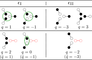
4) Ice rule fragility: mixed coordination. More interesting is the ice rule breakdown in non-trivial, infinite lattices such as lattices of mixed coordination. Consider a regular or random decimation of a trivially equivalent structure such as the hexagonal ice. Because the background of positive dumbbells has no effect in the original geometry, we can express its effect in the decimated geometry as coming from negative virtual dumbbells, i.e. — traps saturated with negative particles, placed in correspondence of the decimated links (Fig. 4).

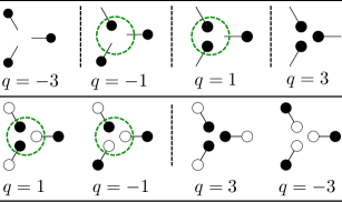
Figure 4: A portion of a decimated, infinitely extended PI (top left) in its low energy state can have ice rule violations on z=2 vertices ($q=+2$, blue circles) because it is equivalent to a SI stuffed with virtual, negatively saturated traps (red, dashed) in lieu of the removed links (top right) with no violations of the ice rule in the virtual charge ($\tilde{q}=\pm 1$). Indeed, while the SI energetics of the undecimated, $z=3$, vertices (middle) is left unchanged, that of the decimated $z=2$ vertices (bottom) must include virtual negative saturated traps, and thus violates the ice rule at lowest energy: the vertex of real charge $q=2$ (virtual charge $\tilde{q}=1$) is degenerate with the vertex of real charge $q=0$ (virtual charge $\tilde{q}=-1$), and with the $z=3$ vertices of real charge $q=\pm 1$ (ice rule vertices circled in dashed green).

Crucially, in a vertex-model approximation the energy of a vertex is proportional to its net virtual charge $\tilde{q}$, inclusive of the charge of the negative, virtual dumbbell — , breaking the $\mathbb{Z}_{2}$ symmetry of the SI energetics. As Fig. 4 shows, in $z=2$ vertices the ice rule violating 2-in/0-out configuration of virtual charge $\tilde{q}=-1$ but real positive charge $q=2$, has the same energy of the ice-rule configuration of 1-in/1-out ($q=0$, $\tilde{q}=+1$), but also of the ice rule configurations of $z=3$ vertices. Thus, $q=2$ charges appear entropically on $z=2$ vertices in the degenerate ground state, in violation of the ice rule. The $z=3$ vertices remain in the ice rule, but $q=-1$ charges must exceed $q=1$ ones, to cancel the positive charge on the $z=2$ vertices.

This argument is completely general. Any mixed coordination lattice that can be obtained from decimating an ice-rule obeying PI must similarly show a transfer of topological charge from vertices of higher coordination to the decimated vertices of lower coordination, where charge is attracted by negative virtual charges. Note that violation of the ice rule, however, do not necessarily happen in the lowest coordination vertices, as shown below and as found recently Libal and et al (2017) in square PI. This charge transfer is unique to PI, and nothing of the sort can happen in SI. There the ice rule is robust to decimation and mixed coordination Morrison et al. (2013); Gilbert et al. (2014); Gilbert et al. (2016a), dislocations Drisko et al. (2017), and indeed even in clusters Li et al. (2010) as it is enforced by the local energy.

Finally, the charge transfer should be associated with glassiness. Indeed, while the average net charge must remain zero, or $q_{\mathrm{net}}\equiv N_{v}^{-1}\sum_{v}\langle q_{v}\rangle=0$ ($N_{v}$ is the number of vertices), its Edwards-Anderson parameter is not, or $q^{2}_{\mathrm{EA}}\equiv N_{v}^{-1}\sum_{v}\langle q_{v}\rangle^{2}\neq 0$, because of the breakdown of the $\mathbb{Z}_{2}$ symmetry in the equivalent PI picture. This implies freezing of the charge in random distributions as $q^{2}_{\mathrm{EA}}$ is also the charge temporal autocorrelation function at large times.

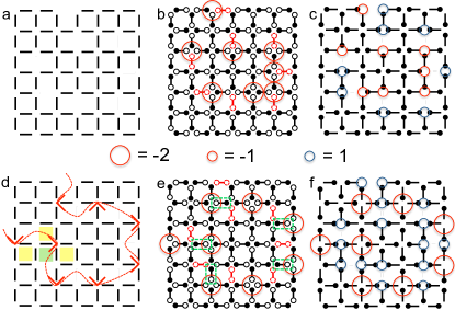
5—Order breakdown from topological charge transfer. It is well known that the ice manifolds of square PI/SI are antiferromagnetically ordered because traps/spins converging perpendicularly in the vertex interact more strongly than those converging collinearly. This lifts the degeneracy of the ice-rule and favors the non-polarized, antiferromagnetic ice rule vertices Wang et al. (2006); Porro et al. (2013); Zhang et al. (2013); Libál et al. (2006) of in Fig. 3. Consider a random decimations of traps in square PI that does not create $z=2$ vertices. It corresponds to a partial cover for a dimer cover model on the edges of the square lattice (Fig. 5a). In SI, such special decimation is expected to preserve the antiferromagnetic order Morrison et al. (2013). In PI, instead, it implies a structural transition to disorder, as shown below.

Consider a decimation of the antiferromagnetic ensemble (Fig. 5b,c). Each virtual negative dumbbell creates a negative virtual monopole $\tilde{q}=-2$ on a $z=3$ vertex. As explained above, the energy depends on the virtual charges. Because of (virtual and real) charge conservation, this decimated antiferromagnetically ordered state, which obeys the ice rule ($z=3$ vertices all have charges $q=\pm 1$) has the lowest energy. Is it unique?

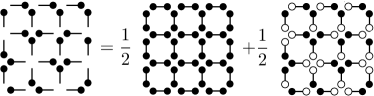
Figure 5: Top (a-c): Decimating a square lattice (a) and its anfiferromagnetic ground state (decimated traps are replaced with negatively saturated traps, in red) leads to an ordered lowest energy state with $\tilde{q}=-2$ virtual charges on half of the decimated vertices in the SI picture (b). It corresponds to $q=\pm 1$ real charges on decimated vertices in the PI picture (c) and thus all vertices obey the ice rule. At low decimation, this is the only low energy state. Bottom (d-f): However, above the decimation threshold corresponding to the percolation of decimated neighboring square plaquettes [e.g. yellow shaded ones neighboring a green one in (a)], the low energy state becomes degenerate. A disordered state can be chosen by connecting (red dotted line) neighboring decimated plaquettes (d) with $q=-2$ monopoles (represented with $\wedge$ connectors as in Fig. 3) on $z=4$ vertices, thus removing the virtual charges from decimated, $z=3$ vertices without increasing the energy [(e), green rectangles frame spins that can be freely flipped]. In the PI picture (f) this corresponds to ice rule violations on the $z=4$ vertices hosting charge $q=2$: disorder comes from entropic transfer of topological charge.

At sufficiently low decimation it clearly is. Indeed, in a low energy state only antiferromagnetic $q=0$ ground state vertices, and $q=-2$ monopoles are allowed on $z=4$ vertices. Therefore, in each minimal plaquette the four dipoles must be arranged head to toe, except in correspondence of a monopole. In a plaquette affected by a virtual trap, a negative virtual charge sits on one of the two decimated vertices if and only if the remaining three spins are arranged head to toe. Antiferromagnetic order can break down if both virtual charges on the two neighboring decimated vertices are $\tilde{q}=0$ (and therefore their real charge is positive, $q=1$, on both). For that to happen, the head to toe rule must be broken on one of the two other vertices in each of the two relative plaquettes. It follows that two monopole of charge $q=-2$ must sit on the rectangular plaquette resulting from the decimation, as monopoles are the only allowed vertices that can beak the head-to-toe rule. Because a monopole breaks the head-to-toe rule on two of the four plaquettes it separates (Fig. 3), this is only possible if at least one of the nearest neighboring plaquette is also decimated (Fig. 5d). Therefore, when the decimation is sufficiently low and the number of neighboring decimated plaquette is non-extensive the decimated antiferromagnetic state is the only ground state. However, when nearest neighboring decimated plaquette percolate (Fig. 5d), the low energy ensemble becomes disordered.

One can prove so by construction. Start with the decimated lattice, connect (or not) any neighboring decimated rectangular plaquette which can be connected via the red $\wedge$-connector of Fig. 5, representing a monopole (Fig. 3). Then all the spins are determined. This construction corresponds to lines threading through decimated plaquettes (red dotted in Fig. 5c). When the decimated plaquettes percolate at the nearest neighbor, these lines can be chosen freely either as closed loops or as infinite paths percolating through the material. This freedom in choosing connecting lines, and more trivially the resulting free spins (Fig. 5e), give a residual entropy to the ground state. There is thus a transition from order to a disordered state at a critical decimation, likely a glassy one involving dynamic arrest, and which invites experimental analysis.

Conclusion. PI can be considered a SI under a local fields that can break the SI’s $\mathbb{Z}_{2}$ symmetry. We have explored some of the implications and novel phenomenology which invite further numerical and experimental analysis. An extension to kinetics will be explored in the future: as the current isomorphism starts from particles in their preferential binary locations it does not capture their motion across the trap, nor their intermediate interactions. Further developments includes the deliberate design of functional structural features, such as interfaces which will accumulate positive charge and be therefore semipermeable to the passage of topologically charged defects under proper fields.

We wish to thank the LDRD office for financial support through the ER program, A Libal, C. Reichhardt and CJ Olson Reichhardt (Los Alamos), and A. Ortiz and P. Tierno (Barcelona) for useful discussions and for sharing preliminary numerical and experimental results. This work was carried out under the auspices of the NNSA of the U.S. DoE at LANL under Contract No. DE-AC52-06NA25396.