Maxwell electrodynamics modified by CPT-even and Lorentz-violating
dimension-6 higher-derivative terms

Abstract

In this paper, we investigate an electrodynamics in which the physical modes are coupled to a Lorentz-violating (LV) background by means of a higher-derivative term. We analyze the modes associated with the dispersion relations (DRs) obtained from the poles of the propagator. More specifically, we study Maxwell’s electrodynamics modified by a LV operator of mass dimension 6. The modification has the form ${D_{\beta\alpha}}\partial_{\sigma}F^{\sigma\beta}\partial_{\lambda}F^{\lambda\alpha}$, i.e., it possesses two additional derivatives coupled to a CPT-even tensor $D_{\beta\alpha}$ that plays the role of the fixed background. We first evaluate the propagator and obtain the dispersion relations of the theory. By doing so, we analyze some configurations of the fixed background and search for sectors where the energy is well-defined and causality is assured. A brief analysis of unitarity is included for particular configurations. Afterwards, we perform the same kind of analysis for a more general dimension-6 model. We conclude that the modes of both Lagrange densities are possibly plagued by physical problems, including causality and unitarity violation, and that signal propagation may become physically meaningful only in the high-momentum regime.

I Introduction

Physics beyond the Standard Model has been under extensive development in the latest years, encompassing Lorentz-violating (LV) theories as one branch of investigation. The minimal Standard-Model Extension (SME) Colladay ; Samuel is a general gauge-invariant and power-counting renormalizable framework that incorporates terms of Lorentz invariance violation by means of tensor-valued background fields fixed under particle Lorentz transformations. These background fields can be interpreted as vacuum expectation values that are generated by spontaneous symmetry breaking taking place in a more fundamental theory. Studies in the SME have been pursued to look for LV effects and to develop a precision programme that allows us to scrutinize the limits of Lorentz symmetry in several physical interactions. In this sense, many investigations were performed in the context of the SME fermion sector Fermion1 ; Fermion2 , CPT-violating contributions CPT , the CPT-odd electromagnetic sector Adam1 ; Cherenkov1 , the CPT-even electromagnetic sector Cherenkov2 ; KM , fermion-photon interactions KFint ; Interac ; Schreck1 , and radiative corrections Radio . Lorentz-violating theories are also connected to higher-dimensional operators. In this sense, nonminimal extensions of the SME were developed, both in the photon Kostelec1 and fermion sector Kostelec2 , composed by CPT-even and CPT-odd higher-derivative operators. Other higher-dimensional LV theories Myers1 ; Marat were also proposed and examined. Nonminimal higher-dimensional couplings that do not involve higher derivatives have been proposed and constrained, as well NModd1 ; NM3 ; NMkost .

Models of a higher-derivative electrodynamics have been investigated since the advent of Podolsky’s theory Podolsky1 , characterized by the Lorentz- and gauge-invariant term $\partial_{\alpha}F^{\alpha\beta}\partial_{\lambda}F^{\lambda}{}_{\beta}$, one of the simplest dimension-6 structures that can be built with the electromagnetic field. Podolsky’s Lagrangian is

$$\mathcal{L}=-\frac{1}{4}F_{\mu\nu}F^{\mu}{}^{\nu}+\frac{\theta^{2}}{2}\partial_{\alpha}F^{\alpha}{}^{\beta}\partial_{\lambda}F_{\phantom{\lambda}\beta}^{\lambda}-j_{\mu}A^{\mu}\,,$$ (1)

where $F_{\mu\nu}=\partial_{\mu}A_{\nu}-\partial_{\nu}A_{\mu}$ is the field strength tensor assigned to the vector field $A_{\mu}$ and $\theta$ is Podolsky’s parameter having mass dimension $-1$. The vector field is coupled to a conserved four-current $j_{\mu}$. One of the most remarkable characteristics of Podolsky’s electrodynamics is the generation of a massive mode without the loss of gauge symmetry, being in this aspect different from Proca’s theory. The Podolsky propagator contains two poles, one corresponding to the massless photon and the other one associated with the massive photon. At the classical level, the massive mode of the model has the advantage of curing divergences connected to the pointlike self-energy, but at the quantum level it is associated with the occurrence of ghosts Accioly1 . The suitable gauge condition to address Podolsky’s electrodynamics is not the usual Lorenz gauge, but a modified gauge relation GalvaoP , compatible with the existence of five degrees of freedom (two related to a massless photon and three related to the massive mode). Other aspects of quantum field theories in the presence of the Podolsky term, such as path integral quantization and finite-temperature effects Podolsky3 ; Podolsky4 , renormalization Podolsky5 , as well as multipole expansion and classical solutions Podolsky6 were also examined.

Another dimension-6 term, proposed in the late sixties, $F_{\mu\nu}\partial_{\alpha}\partial^{\alpha}F^{\mu\nu}$, defines Lee-Wick electrodynamics LeeWick , which leads to a finite self-energy for a pointlike charge in (1+3) spacetime dimensions. Furthermore, it produces a bilinear contribution to the Lagrangian similar to that of Podolsky’s term but with opposite sign. This “wrong” sign yields energy instabilities at the classical level, while it leads to negative-norm states in the Hilbert space at the quantum level. Lee and Wick also proposed a mechanism to preserve unitarity, which removes all states containing Lee-Wick photons from the Hilbert space. This theory regained attention after the proposal of the Lee-Wick standard model LW , based on a non-Abelian gauge structure free of quadratic divergences. Such a model had a broad repercussion, with many contributions in both the theoretical and phenomenological sense LW2 . In the Lee-Wick scenario, studies of ghost states LWghost , constructions endowed with higher derivatives LWhd , renormalization aspects LWren , and finite-temperature investigations LWft have been reported, as well. The study of higher-derivative terms in quantum field theories was also motivated by their role as ultraviolet regulators A.A . Some works were dedicated to investigating interactions between stationary sources in the context of Abelian Lee-Wick models, with emphasis on sources distributed along parallel branes with arbitrary dimension and the Dirac string in such a context Barone1 . Lee-Wick electrodynamics was also studied for the case of the self-energy of pointlike charges in arbitrary dimensions, exhibiting a finite ultraviolet result for $d=1$ and $d=3$ (spatial dimensions) Barone2 , for the case of perfectly conducting plates Barone3 , and in the evaluation of the interaction between two pointlike charges Accioly2 . Recently, a LV higher-derivative and dimension-6 term, $d_{\beta}d_{\sigma}\partial_{\alpha}F^{\alpha}{}^{\beta}\partial_{\lambda}F^{\lambda\sigma}$ with an observer four-vector $d_{\mu}$, radiatively generated in Ref. Petrov , was considered in the context of Maxwell’s Lagrangian Barone4 . The latter study focused on interactions between external sources with the modified electromagnetic field, as performed in Refs. Barone1 ; Barone2 .

For almost 20 years now, Lorentz-violating contributions of mass dimensions 3 and 4 have been investigated extensively from both a phenomenological and a theoretical point of view. Many of the corresponding controlling coefficients are tightly constrained, especially in the photon and lepton sector Kostelecky:2008ts . Since a point in time not long ago, a significant interest was aroused in field theories endowed with higher-order derivatives. In the CPT-even photon sector, the leading-order contributions in an expansion in terms of additional derivatives are the dimension-6 ones. Hence, these are also the most prominent ones that could play a role in nature, if higher-derivative Lorentz violation existed. Note that Lorentz-violating terms of mass dimension 6 are known to emerge from theories of noncommutative spacetimes, as the noncommutativity tensor has a mass dimension of $-2$.

In the present work, we investigate basic features of a higher-derivative electrodynamics, in which the physical fields are coupled to a CPT-even and LV background by means of a dimension-6 term. More specifically, we study Maxwell’s theory modified by a LV operator of mass dimension 6, which possesses two additional derivatives coupled to a CPT-even fixed background, $D_{\beta\alpha}$, in a structure of the form ${D_{\beta\alpha}}\partial_{\sigma}F^{\sigma\beta}\partial_{\lambda}F^{\lambda\alpha}$. The latter is a kind of anisotropic Podolsky term, i.e., it is a natural Lorentz-violating extension of Podolsky’s theory. Initially, the condition is discussed (nonzero trace) for which a LV structure of this kind comprises the Podolsky term. It is interesting to note that in the recent article Bonetti:2016vrq , Lorentz violation is considered in a scenario with intact supersymmetry. The Lorentz-violating background fields are assumed to be linked to a supersymmetric multiplet and their effect on photon propagation is studied. After integrating out the contributions from the photino, the effective Lagrangian given by their Eq. (9) incorporates the type of modified Podolsky term that we are studying.

So far, not much is known about the properties of Lorentz-violating theories including higher derivatives. It is a well-established fact, though, that higher-dimensional operators lead to a rich plethora of new effects as well as additional issues. For example, the existence of additional time derivatives may produce exotic modes that cannot be considered as perturbations of the standard ones. These modes can lead to an indefinite metric in Hilbert space, which is connected to the occurrence of states with negative norm. The procedure developed by Lee and Wick LeeWick makes it possible to deal with such modes in a quantized theory such that a breakdown of unitarity is prevented. Before delving into these possibly very profound problems of Lorentz-violating theories including higher derivatives, the classical properties of these frameworks should be well understood first.

Describing classical aspects of LV theories with higher derivatives is the main motivation of the current paper. Hence, we are interested in obtaining the Green’s function of the field equations and the dispersion relations as well as developing an understanding of classical causality. Using a technique already employed in some previous LV models Propagator , which consists of finding a closed projector algebra, and using the prescription $D_{\mu\nu}=({B_{\mu}}C_{\nu}+{B_{\nu}}C_{\mu})/2$ with two observer four-vectors $B_{\mu}$ and $C_{\mu}$, the propagator is derived and the dispersion relations are determined from its poles. The goal of this work is to examine signal propagation within a Podolsky electrodynamics modified by the term ${D_{\beta\alpha}}\partial_{\sigma}F^{\sigma\beta}\partial_{\lambda}F^{\lambda\alpha}$. Thus, the modes described by the corresponding dispersion relations are analyzed for several configurations of the fixed background and we search for sectors where the energy is well-defined and causality is assured. Furthermore, we will perform a brief analysis of unitarity of the theory for a vanishing Podolsky parameter. After doing so, we present a more general dimension-6 higher-derivative Lagrangian that can be proposed in the presence of the rank-2 background $D_{\beta\alpha}$. The latter also involves a kind of anisotropic Lee-Wick term ${D^{\mu\nu}}\partial_{\sigma}F^{\sigma\lambda}\partial_{\mu}F_{\nu\lambda}$. The corresponding propagator and the dispersion relations are derived again. Mode propagation is examined for several configurations of the background, revealing that the dispersion relations of these LV dimension-6 model may exhibit a physical behavior in the limit of large momenta only. We finally show that the dimension-6 terms considered here are contained in the nonminimal SME developed by Kostelecký and Mewes Kostelec1 . Throughout the paper, natural units will be employed with $\hbar=c=1$.

II Maxwell electrodynamics modified by higher-derivative terms: some possibilities

As a first step, we propose a Maxwell electrodynamics modified by a higher-derivative, CPT-even term of mass dimension 6 including two additional derivatives coupled to a fixed tensor $D_{\beta\alpha},$ that is,

$${D_{\beta\alpha}}\partial_{\sigma}F^{\sigma}{}^{\beta}\partial_{\lambda}F^{\lambda}{}^{\alpha}\,,$$ (2)

which represents a kind of anisotropic and generalized Podolsky term. Without a restriction of generality, $D_{\beta\alpha}$ can be taken to be symmetric, as its antisymmetric part does not contribute, anyhow. Hence, a possible Lagrangian to be considered is

$$\mathcal{L}=-\frac{1}{4}F_{\mu\nu}F^{\mu}{}^{\nu}+\eta^{2}{D_{\beta\alpha}}\partial_{\sigma}F^{\sigma}{}^{\beta}\partial_{\lambda}F^{\lambda}{}^{\alpha}\,,$$ (3)

where the parameter $\eta$ has dimension of (mass)${}^{\text{--1}}$. A property to check is if the anisotropic piece (2) contains a sector that is equivalent to the Podolsky term of Eq. (1). Such a term is generated from a nonvanishing trace of $D_{\mu\nu}$, what can be shown quickly. If $D_{\mu\nu}$ contains nonzero diagonal components of the form $D_{11}=D_{22}=D_{33}=-D_{00}$, the tensor involves a trace that is given by

$${D^{\lambda}_{\phantom{\lambda}\lambda}}=D_{00}-D_{ii}=4D_{00}\,.$$ (4)

We define a new traceless tensor $\tilde{D}_{\beta\alpha}$ by subtracting the trace from the latter:

$${\tilde{D}_{\beta\alpha}\equiv D_{\beta\alpha}-\frac{1}{4}g_{\beta\alpha}D^{\rho}_{\phantom{\rho}\rho}=D_{\beta\alpha}-g_{\beta\alpha}D_{00}\,,}$$ (5)

which fulfills $\tilde{D}^{\kappa}_{\phantom{\kappa}\kappa}=0$ and leads to

$${\tilde{D}_{\beta\alpha}}\partial_{\sigma}F^{\sigma}{}^{\beta}\partial_{\lambda}F^{\lambda\alpha}={D_{\beta\alpha}}\partial_{\sigma}F^{\sigma}{}^{\beta}\partial_{\lambda}F^{\lambda\alpha}-{D_{00}(\partial_{\sigma}F^{\sigma}{}^{\beta}\partial_{\lambda}F_{\phantom{\lambda}\beta}^{\lambda})}\,.$$ (6)

The second term on the right-hand side corresponds to a Podolsky term, i.e., such a term appears in connection to the trace of $D_{\mu\nu}$, indeed. In this sense, there are two possibilities that can be pursued, i.e., we can assess a dimension-6 electrodynamics that either contains or does not contain the Podolsky term. One option that exhibits, in principle, the same physical content of Lagrangian (3) is to consider Podolsky’s electrodynamics modified by the traceless LV dimension-6 term of Eq. (5), that is,

$$\mathcal{L}=-\frac{1}{4}F_{\mu\nu}F^{\mu}{}^{\nu}+\frac{\theta^{2}}{2}\partial_{\alpha}F^{\alpha}{}^{\beta}\partial_{\lambda}F_{\phantom{\lambda}\beta}^{\lambda}+\eta^{2}{\tilde{D}_{\beta\alpha}}\partial_{\sigma}F^{\sigma}{}^{\beta}\partial_{\lambda}F^{\lambda}{}^{\alpha}\,.$$ (7)

A cleaner option including only the LV dimension-6 contribution in the context of Maxwell’s electrodynamics, is defined when the Podolsky sector is zero, $D^{\kappa}_{\phantom{\kappa}\kappa}=0$, so that the Lagrangian to be addressed is

$$\mathcal{L}=-\frac{1}{4}F_{\mu\nu}F^{\mu}{}^{\nu}+\eta^{2}{\tilde{D}_{\beta\alpha}}\partial_{\sigma}F^{\sigma}{}^{\beta}\partial_{\lambda}F^{\lambda}{}^{\alpha}\,.$$ (8)

	$C$	$P$	$T$	CPT
$D_{00}$	$+$	$+$	$+$	$\ +$
$D_{0i}$	$+$	$-$	$-$	$\ +$
$D_{ij}$	$+$	$+$	$+$	$\ +$

Table 1: Transformation properties of the components of $D_{\mu\nu}$ under C, P, T and their combination.

The components of the tensor $D_{\beta\alpha}$ can be classified in accordance with the behavior under the discrete C, P, and T operations. To do so, we decompose the sum over the contracted indices in the term (2) into components of the electric and magnetic fields $\mathbf{E}$, $\mathbf{B}$:

$${D_{\beta\alpha}}\partial_{\sigma}F^{\sigma}{}^{\beta}\partial_{\lambda}F^{\lambda}{}^{\alpha} ={D_{00}}\partial_{a}E^{a}{}\partial_{b}E^{b}{}-2\epsilon^{bil}{D_{0i}}\partial_{a}E^{a}{}\partial_{b}B^{l}$$

$$\phantom{{}={}}-2{D_{0i}}\partial_{a}E^{a}{}\partial_{0}E{}^{i}+{D_{ij}}\partial_{0}E{}^{i}\partial_{0}E{}^{j}$$

$$\phantom{{}={}}+2\epsilon^{bjl}{D_{ij}}\partial_{0}E{}^{i}\partial_{b}B^{l}+\epsilon^{bjl}\epsilon^{aim}{D_{ij}}\partial_{a}B^{m}\partial_{b}B^{l}\,,$$ (9)

remembering that $F^{a0}{}=E^{a},F^{b}{}^{j}=-\epsilon^{bjl}B^{l}$ with the three-dimensional Levi-Civita symbol $\epsilon^{ijk}$. Under charge conjugation (C), the electric and magnetic fields behave according to $\mathbf{E}\rightarrow-\mathbf{E}$ and $\mathbf{B}\rightarrow-\mathbf{B},$ while $\partial_{\mu}\rightarrow\partial_{\mu}.$ In this way, we notice that the coefficients $D_{00},D_{0i},D_{ij}$ are C-even. Under parity (P), $\mathbf{E}\rightarrow-\mathbf{E}$ and $\mathbf{B}\rightarrow\mathbf{B}$, $\partial_{a}\rightarrow-\partial_{a},\partial_{0}\rightarrow\partial_{0},$ so that $D_{0i}$ is parity-odd, and $D_{00}$ and $D_{ij}$ are parity-even. Under time reversal ($T),$ $\mathbf{B}\rightarrow-\mathbf{B}$, $\mathbf{E}\rightarrow\mathbf{E}$, with $\partial_{a}\rightarrow\partial_{a},\partial_{0}\rightarrow-\partial_{0}.$ This implies that $D_{0i}$ is $T$-odd, while $D_{00}$ and $D_{ij}$ are T-even. A summary of these properties can be found in Tab. 1.

III Propagator of the dimension-6 generalized Podolsky theory

In this section, we consider the Maxwell Lagrangian modified by the Podolsky and the dimension-6 anisotropic higher-derivative term (2), given as

$$\mathcal{L}=-\frac{1}{4}F_{\mu\nu}F^{\mu}{}^{\nu}+\frac{\theta^{2}}{2}\partial_{\alpha}F^{\alpha}{}^{\beta}\partial_{\lambda}F_{\phantom{\lambda}\beta}^{\lambda}+\eta^{2}D_{\beta\alpha}\partial_{\sigma}F^{\sigma}{}^{\beta}\partial_{\lambda}F^{\lambda\alpha}{}+\frac{1}{2\xi}\left(\partial_{\mu}A^{\mu}\right)^{2}\,,$$ (10)

where the last contribution is introduced to fix the gauge. The parameters $\theta$, $\eta$ have dimension of (mass)${}^{\text{--1}}$ and $D_{\beta\alpha}$ is the dimensionless CPT-even tensor introduced before. The coefficients $\theta^{2}$ and $\eta^{2}$ are here considered as positive in analogy with Podolsky’s theory, where $\theta^{2}>0$ is a necessary condition for obtaining a physical dispersion relation. In a broad context, there exists the possibility of considering $\theta^{2}$ and $\eta^{2}$ as negative. These choices have the potential for altering dispersion relations and other physical properties of the theory such as unitarity. However, an investigation of this sector is beyond the scope of the paper, which is why we will assume that both $\theta^{2}\geq 0$ and $\eta^{2}\geq 0$. The Lagrangian (10) can be written in the bilinear form,

$$\mathcal{L}=\frac{1}{2}A^{\nu}O_{\mu\nu}A^{\mu}\,,$$ (11)

where $O_{\mu\nu}$ is

$$O_{\mu\nu} ={(1+\theta^{2}\square)\square\Theta_{\mu\nu}}-\frac{1}{\xi}\square\Omega_{\mu\nu}$$

$$\phantom{{}={}}+2\eta^{2}[{D_{\nu\mu}}\square^{2}-{D_{\nu\alpha}}\square\partial_{\mu}\partial^{\alpha}-{D_{\sigma\mu}}\square\partial_{\nu}\partial^{\sigma}+{D_{\sigma\alpha}}\partial_{\nu}\partial_{\mu}\partial^{\sigma}\partial^{\alpha}]\,.$$ (12)

$$\begin{array}[c]{cccccc}\hline\cr\hline\cr&\Theta_{\phantom{\nu}\alpha}^{\nu}&\Omega_{\phantom{\nu}\alpha}^{\nu}&B_{\alpha}\partial^{\nu}&B_{\alpha}C^{\nu}&C^{\nu}\partial_{\alpha}\\ \hline\cr\Theta_{\mu\nu}&\Theta_{\mu\alpha}&0&0&B_{\alpha}C_{\mu}-\frac{\rho}{\square}B_{\alpha}\partial_{\mu}&C_{\mu}\partial_{\alpha}-\rho\Omega_{\mu\alpha}\\ \hline\cr\Omega_{\mu\nu}&0&\Omega_{\mu\alpha}&B_{\alpha}\partial_{\mu}&\frac{\rho}{\square}B_{\alpha}\partial_{\mu}&\rho\Omega_{\mu\alpha}\\ \hline\cr B_{\nu}\partial_{\mu}&B_{\alpha}\partial_{\mu}-\kappa\Omega_{\mu\alpha}&\kappa\Omega_{\mu\alpha}&\kappa B_{\alpha}\partial_{\mu}&(B\cdot C)B_{\alpha}\partial_{\mu}&(B\cdot C)\square\Omega_{\mu\alpha}\\ \hline\cr B_{\nu}C_{\mu}&B_{\alpha}C_{\mu}-\frac{\kappa}{\square}C_{\mu}\partial_{\alpha}&\frac{\kappa}{\square}C_{\mu}\partial_{\alpha}&\kappa B_{\alpha}C_{\mu}&(B\cdot C)B_{\alpha}C_{\mu}&(B\cdot C)C_{\mu}\partial_{\alpha}\\ \hline\cr C_{\mu}\partial_{\nu}&0&C_{\mu}\partial_{\alpha}&\square B_{\alpha}C_{\mu}&\rho B_{\alpha}C_{\mu}&\rho C_{\mu}\partial_{\alpha}\\ \hline\cr B_{\mu}\partial_{\nu}&0&B_{\mu}\partial_{\alpha}&\square B_{\mu}B_{\alpha}&\rho B_{\mu}B_{\alpha}&\rho B_{\mu}\partial_{\alpha}\\ \hline\cr B_{\mu}C_{\nu}&B_{\mu}C_{\alpha}-\frac{\rho}{\square}B_{\mu}\partial_{\alpha}&\frac{\rho}{\square}B_{\mu}\partial_{\alpha}&\rho B_{\mu}B_{\alpha}&C^{2}B_{\mu}B_{\alpha}&C^{2}B_{\mu}\partial_{\alpha}\\ \hline\cr C_{\nu}\partial_{\mu}&C_{\alpha}\partial_{\mu}-\rho\Omega_{\mu\alpha}&\rho\Omega_{\mu\alpha}&\rho B_{\alpha}\partial_{\mu}&C^{2}B_{\alpha}\partial_{\mu}&C^{2}\square\Omega_{\mu\alpha}\\ \hline\cr B_{\mu}B_{\nu}&B_{\mu}B_{\alpha}-\frac{\kappa}{\square}B_{\mu}\partial_{\alpha}&\frac{\kappa}{\square}B_{\mu}\partial_{\alpha}&\kappa B_{\mu}B_{\alpha}&(B\cdot C)B_{\mu}B_{\alpha}&(B\cdot C)B_{\mu}\partial_{\alpha}\\ \hline\cr C_{\mu}C_{\nu}&C_{\mu}C_{\alpha}-\frac{\rho}{\square}C_{\mu}\partial_{\alpha}&\frac{\rho}{\square}C_{\mu}\partial_{\alpha}&\rho B_{\alpha}C_{\mu}&C^{2}B_{\alpha}C_{\mu}&C^{2}C_{\mu}\partial_{\alpha}\\ \hline\cr\hline\cr\end{array}$$

Table 2: Closed algebra of tensor projectors (part 1).

Here, we have used the longitudinal and transverse projectors,

$$\Omega_{\beta\lambda}=\frac{\partial_{\beta}\partial_{\lambda}}{\square}\,,\quad\Theta_{\beta\lambda}=g_{\beta\lambda}-\Omega_{\beta\lambda}\,,$$ (13)

respectively, where $g_{\mu\nu}$ is the Minkowski metric with signature $(+,-,-,-)$. To derive the propagator, we propose the following parameterization:

$$D_{\mu\nu}=\frac{1}{2}({B_{\mu}}C_{\nu}+{B_{\nu}}C_{\mu})\,,$$ (14)

where $C_{\mu},B_{\nu}$ are two independent observer four-vectors giving rise to preferred spacetime directions. This parameterization is nearly general and describes most of the configurations of the symmetric $D_{\beta\alpha}$ tensor. It is used for technical reasons, mainly connected to the construction of the propagator of this theory. Furthermore, it allows us to classify different sectors of the theory by geometric properties related to the two vectors, e.g., orthogonality of their spatial parts. With the latter choice, the operator of Eq. (12) becomes

$$O_{\mu\nu} =(1+\theta^{2}\square)\square\Theta_{\mu\nu}+\left(2\eta^{2}{\kappa\rho}-\frac{1}{\xi}\right)\square\Omega_{\mu\nu}+\eta^{2}{(B_{\mu}C_{\nu}+B_{\nu}C_{\mu})}\square^{2}$$

$$\phantom{{}={}}-\eta^{2}\square({C_{\nu}}\kappa\partial_{\mu}+{C_{\mu}}\kappa\partial_{\nu}+{B_{\nu}}\rho\partial_{\mu}+{B_{\mu}}\rho\partial_{\nu})\,,$$ (15)

with

$$\kappa=B_{\alpha}\partial^{\alpha}\,,\quad\rho=C_{\alpha}\partial^{\alpha}\,.$$ (16)

$$\begin{array}[c]{cccccc}\hline\cr\hline\cr&B^{\nu}\partial_{\alpha}&B^{\nu}C_{\alpha}&C_{\alpha}\partial^{\nu}&B^{\nu}B_{\alpha}&C^{\nu}C_{\alpha}\\ \hline\cr\Theta_{\mu\nu}&B_{\mu}\partial_{\alpha}-\kappa\Omega_{\mu\alpha}&B_{\mu}C_{\alpha}-\frac{\kappa}{\square}C_{\alpha}\partial_{\mu}&0&B_{\mu}B_{\alpha}-\frac{\kappa}{\square}B_{\alpha}\partial_{\mu}&C_{\mu}C_{\alpha}-\frac{\rho}{\square}C_{\alpha}\partial_{\mu}\\ \hline\cr\Omega_{\mu\nu}&\kappa\Omega_{\mu\alpha}&\frac{\kappa}{\square}C_{\alpha}\partial_{\mu}&C_{\alpha}\partial_{\mu}&\frac{\kappa}{\square}B_{\alpha}\partial_{\mu}&\frac{\rho}{\square}C_{\alpha}\partial_{\mu}\\ \hline\cr B_{\nu}\partial_{\mu}&\square B^{2}\Omega_{\mu\alpha}&B^{2}C_{\alpha}\partial_{\mu}&\kappa C_{\alpha}\partial_{\mu}&B^{2}B_{\alpha}\partial_{\mu}&(B\cdot C)C_{\alpha}\partial_{\mu}\\ \hline\cr B_{\nu}C_{\mu}&B^{2}C_{\mu}\partial_{\alpha}&B^{2}C_{\mu}C_{\alpha}&\kappa C_{\mu}C_{\alpha}&B^{2}B_{\alpha}C_{\mu}&(B\cdot C)C_{\mu}C_{\alpha}\\ \hline\cr C_{\mu}\partial_{\nu}&\kappa C_{\mu}\partial_{\alpha}&\kappa C_{\mu}C_{\alpha}&\square C_{\mu}C_{\alpha}&\kappa B_{\alpha}C_{\mu}&\rho C_{\mu}C_{\alpha}\\ \hline\cr B_{\mu}\partial_{\nu}&\kappa B_{\mu}\partial_{\alpha}&\kappa B_{\mu}C_{\alpha}&\square B_{\mu}C_{\alpha}&\kappa B_{\mu}B_{\alpha}&\rho B_{\mu}C_{\alpha}\\ \hline\cr B_{\mu}C_{\nu}&(B\cdot C)B_{\mu}\partial_{\alpha}&(B\cdot C)B_{\mu}C_{\alpha}&\rho B_{\mu}C_{\alpha}&(B\cdot C)B_{\mu}B_{\alpha}&C^{2}B_{\mu}C_{\alpha}\\ \hline\cr C_{\nu}\partial_{\mu}&\square(B\cdot C)\Omega_{\mu\alpha}&(B\cdot C)C_{\alpha}\partial_{\mu}&\rho C_{\alpha}\partial_{\mu}&(B\cdot C)B_{\alpha}\partial_{\mu}&C^{2}C_{\alpha}\partial_{\mu}\\ \hline\cr B_{\mu}B_{\nu}&B^{2}B_{\mu}\partial_{\alpha}&B^{2}B_{\mu}C_{\alpha}&\kappa B_{\mu}C_{\alpha}&B^{2}B_{\mu}B_{\alpha}&(B\cdot C)B_{\mu}C_{\alpha}\\ \hline\cr C_{\mu}C_{\nu}&(B\cdot C)C_{\mu}\partial_{\alpha}&(B\cdot C)C_{\mu}C_{\alpha}&\rho C_{\mu}C_{\alpha}&(B\cdot C)B_{\alpha}C_{\mu}&C^{2}C_{\mu}C_{\alpha}\\ \hline\cr\hline\cr\end{array}$$

Table 3: Closed algebra of tensor projectors (part 2).

To derive the propagator, we need to invert the operator $O_{\mu\nu},$ composed of the projectors $\Theta_{\mu\nu}$, $\Omega_{\mu\nu}$, $B_{\nu}\partial_{\mu}$, $B_{\mu}\partial_{\nu}$, $C_{\mu}B_{\nu}$, $C_{\nu}B_{\mu}$, $C_{\mu}\partial_{\nu}$, $C_{\nu}\partial_{\mu}$. In this sense, the Ansatz

$$\Delta_{\phantom{\nu}\alpha}^{\nu} =a\Theta_{\phantom{\nu}\alpha}^{\nu}+b\Omega_{\phantom{\nu}\alpha}^{\nu}+cB_{\alpha}\partial^{\nu}+dC^{\nu}B_{\alpha}+eC^{\nu}\partial_{\alpha}$$

$$\phantom{{}={}}+fB^{\nu}\partial_{\alpha}+gC_{\alpha}B^{\nu}+hC_{\alpha}\partial^{\nu}+iB^{\nu}B_{\alpha}+jC^{\nu}C_{\alpha}\,,$$ (17)

for the Green’s function $\Delta_{\nu\alpha}=\Delta_{\nu\alpha}(x-y)$ is proposed obeying the condition, $O_{\mu\nu}\Delta_{\text{ }}^{\nu\alpha}=\delta_{\mu}^{\phantom{\mu}\alpha},$ or

$$O_{\mu\nu}\Delta_{\phantom{\nu}\alpha}^{\nu}=\Theta_{\mu\alpha}+\Omega_{\mu\alpha}\,.$$ (18)

The tensor projectors contained in Eq. (17) fulfill a closed algebra, as shown in Tabs. 2, 3. By inserting Eq. (17) into Eq. (18), we obtain a system of ten equations for the ten coefficients to be determined, whose solution is given by

$$a =\frac{1}{\square(1+\theta^{2}\square)}\,,\quad c=f=\frac{\eta^{4}({C^{2}}\square-\rho^{2}){\kappa}-\eta^{2}\rho\Pi}{\Gamma\square(1+\theta^{2}\square)}\,,$$ (19a)

$$b =-\frac{\xi}{\square}+\frac{\eta^{2}\left[-\eta^{2}\rho^{2}({B^{2}}\square-\kappa^{2})-\eta^{2}\kappa^{2}({C^{2}}\square-\rho^{2})+2{\kappa\rho}\Pi\right]}{\Gamma\square(1+\theta^{2}\square)}\,,$$ (19b)

$$d =g=\frac{\eta^{2}\Pi}{(1+\theta^{2}\square)\Gamma}\,,\quad e=h=\eta^{2}\frac{[\eta^{2}\rho({B^{2}}\square-\kappa^{2})-{\kappa}\Pi]}{\Gamma\square(1+\theta^{2}\square)}\,,$$ (19c)

$$i =-\frac{\eta^{4}({C^{2}}\square-\rho^{2})}{\Gamma(1+\theta^{2}\square)}\,,\quad j=-\frac{\eta^{4}({B^{2}}\square-\kappa^{2})}{\Gamma(1+\theta^{2}\square)}\,,$$ (19d)

where

$$\Gamma =\eta^{4}({B^{2}}\square-\kappa^{2})({C^{2}}\square-\rho^{2})-\Pi^{2},$$ (20a)

$$\Pi =1+\theta^{2}\square+\eta^{2}{(B\cdot C)}\square-\eta^{2}{\kappa\rho}\,.$$ (20b)

In momentum space, the propagator is

$$\Delta_{\nu\alpha} =-\frac{\mathrm{i}}{p^{2}(1-\theta^{2}p^{2})\Gamma(p)}\Big{\{}\Gamma(p)\Theta_{\nu\alpha}+\left[b^{\prime}-\xi(1-\theta^{2}p^{2})\Gamma(p)\right]\Omega_{\nu\alpha}$$

$$\phantom{{}={}-p^{2}(1-\theta^{2}p^{2})\Gamma(p)\big{\{}}-\mathrm{i}F(p)(B_{\nu}p_{\alpha}+B_{\alpha}p_{\nu})-2\eta^{2}{D_{\nu\alpha}}p^{2}\Pi(p)-\mathrm{i}H(p)(C_{\nu}p_{\alpha}+C_{\alpha}p_{\nu})$$

$$\phantom{{}={}-p^{2}(1-\theta^{2}p^{2})\Gamma(p)\big{\{}}\left.+\,\eta^{4}p^{2}{B_{\nu}B_{\alpha}}\left[(C\cdot p)^{2}-{C^{2}}p^{2}\right]+\eta^{4}p^{2}{C_{\nu}C_{\alpha}}\left[(B\cdot p)^{2}-{B^{2}}p^{2}\right]\right\}\,,$$ (21)

where $p_{\mu}$ is the four-momentum and

$$b^{\prime} =\eta^{2}\left\{\eta^{2}(C\cdot p)^{2}\left[(B\cdot p)^{2}-{B^{2}}p^{2}\right]\right.$$ (22a)

$$\phantom{{}={}\eta^{2}\big{\{}}\left.+\,\eta^{2}(B\cdot p)^{2}\left[(C\cdot p)^{2}-{C^{2}}p^{2}\right]-2{(B\cdot p)}(C\cdot p)\Pi(p)\right\}\,,$$

$$F(p) =\mathrm{i}\eta^{2}{(C\cdot p)}\Pi(p)-\mathrm{i}\eta^{4}(B\cdot p)\left[(C\cdot p)^{2}-{C^{2}}p^{2}\right]\,,$$ (22b)

$$H(p) =\mathrm{i}\eta^{2}(B\cdot p)\Pi(p)-\mathrm{i}\eta^{4}(C\cdot p)\left[(B\cdot p)^{2}-{B^{2}}p^{2}\right]\,,$$ (22c)

with

$$\Gamma(p) =\eta^{4}{\left[(B\cdot p)^{2}-B^{2}p^{2}\right]}\left[(C\cdot p)^{2}-{C^{2}}p^{2}\right]-\Pi^{2}(p)\,,$$ (23a)

$$\Pi(p) =1-\theta^{2}p^{2}-\eta^{2}{(B\cdot C)}p^{2}+\eta^{2}{(B\cdot p)}(C\cdot p)\,.$$ (23b)

Note that $$F H \Gamma \Pi \eta=0$$ and have dimensions of (mass)^-1, while and are dimensionless. In the absence of the LV term, , and the propagator (21) takes the form,

$$\Delta_{\nu\alpha}=-\mathrm{i}\left(\frac{\Theta_{\nu\alpha}}{p^{2}(1-\theta^{2}p^{2})}-\frac{\xi}{p^{2}}\Omega_{\nu\alpha}\right)\,,$$ (24)

recovering Podolsky’s propagator, as expected. Setting $\theta^{2}=0$ in the propagator (21), the result is

$$\Delta_{\nu\alpha} =-\frac{\mathrm{i}}{p^{2}\Gamma(p)}\Big{\{}\Gamma(p)\Theta_{\nu\alpha}+(b^{\prime}-\xi\Gamma)\Omega_{\nu\alpha}$$

$$\phantom{{}={}-p^{2}\Gamma(p)}\,-\mathrm{i}F(p)(B_{\nu}p_{\alpha}+B_{\alpha}p_{\nu})-2\eta^{2}{D_{\nu\alpha}}p^{2}\Pi(p)-\mathrm{i}H(p)(C_{\nu}p_{\alpha}+C_{\alpha}p_{\nu})$$

$$\phantom{{}={}-p^{2}\Gamma(p)}\left.\,+\,\eta^{4}{B_{\nu}B_{\alpha}}\left[(C\cdot p)^{2}-{C^{2}}p^{2}\right]{p^{2}}+\eta^{4}{C_{\nu}C_{\alpha}}\left[(B\cdot p)^{2}-{B^{2}}p^{2}\right]{p^{2}}\right\}\,,$$ (25)

where $b^{\prime},F\left(p\right),H\left(p\right),\Gamma\left(p\right)$ are given by the same expressions of Eqs. (22), (60), with

$$\Pi_{\theta=0}(p)=1-\eta^{2}{(B\cdot C)}p^{2}+\eta^{2}{(B\cdot p)}(C\cdot p)\,.$$ (26)

In this situation there are still two poles, $p^{2}=0,$ $\Gamma\left(p\right)=0,$ associated with the Maxwell modes and those related to the LV higher-derivative term. Thus, in principle, the Lagrangian (25) has degrees of freedom linked to both modes, yielding a counting of modes analogue to that in Podolsky’s electrodynamics (see Ref. GalvaoP ).

III.1 Dispersion relations

The dispersion equations of the modified electrodynamics defined by Eq. (10) can be red off the poles of the propagator (21) in momentum space,

$$p^{2}(1-\theta^{2}p^{2}) =0\,,$$ (27a)

$$\Gamma(p) =0\,.$$ (27b)

Since these poles also appear in terms that are not connected to the gauge fixing parameter $\xi$, they must be physical. As before, the dispersion equation $p^{2}=0$ represents the well-known Maxwell modes, while $1-\theta^{2}p^{2}=0$ stands for the Podolsky modes. Both are not modified by the higher-derivative term, whose effect is fully encoded in the dispersion equation (27b). In the absence of the Podolsky term, $\theta^{2}=0,$ the modified Eq. (27b) yields:

$$\eta^{4}{\left[(B\cdot p)^{2}-B^{2}p^{2}\right]\left[(C\cdot p)^{2}-C^{2}p^{2}\right]}-\left[1-\eta^{2}{(B\cdot C)}p^{2}+\eta^{2}{(B\cdot p)}(C\cdot p)\right]^{2}=0\,.$$ (28)

With the help of FORM Vermaseren:2000nd , the dispersion equations above can be generalized to an arbitrary choice of $D_{\mu\nu}$. For a general choice of this tensor, the dispersion equation $p^{2}=0$ remains, but $1-\theta^{2}p^{2}=0$ and Eq. (28) merge into a single equation. Although, in principle, there are many possibilities of forming observer Lorentz scalars from a general two-tensor and the momentum four-vector, the latter result collapses when taking into account that $D_{\mu\nu}$ is symmetric. The equation can then be conveniently written as follows:

$$0 =-\,(1-\theta^{2}p^{2})^{3}-2(1-\theta^{2}p^{2})^{2}\eta^{2}(D_{\mu\nu}p^{\mu}p^{\nu}-p^{2}D^{\mu}_{\phantom{\mu}\mu})$$

$$\phantom{{}={}}+2(1-\theta^{2}p^{2})p^{2}\eta^{4}\left[p^{2}D_{\mu\nu}D^{\mu\nu}-2D_{\mu\nu}D^{\mu\varrho}p^{\nu}p_{\varrho}+D^{\mu}_{\phantom{\mu}\mu}\left(2D_{\nu\varrho}p^{\nu}p^{\varrho}-p^{2}D^{\nu}_{\phantom{\nu}\nu}\right)\right]$$

$$\phantom{{}={}}+\frac{4}{3}p^{4}\eta^{6}\left[3D_{\mu\nu}D^{\mu\nu}\left(D_{\varrho\sigma}p^{\varrho}p^{\sigma}-p^{2}D^{\varrho}_{\phantom{\varrho}\varrho}\right)+(D^{\mu}_{\phantom{\mu}\mu})^{2}\left(p^{2}D^{\nu}_{\phantom{\nu}\nu}-3D_{\nu\varrho}p^{\nu}p^{\varrho}\right)\right.$$

$$\phantom{{}={}+\frac{4}{3}p^{4}\eta^{6}\Big{[}}\left.+\,2p^{2}D^{\mu\nu}D_{\mu}^{\phantom{\mu}\varrho}D_{\nu\varrho}+6\left(D_{\mu\nu}D^{\mu\varrho}p^{\nu}p_{\varrho}D^{\sigma}_{\phantom{\sigma}\sigma}-D_{\mu\nu}D^{\mu\varrho}D^{\nu\sigma}p_{\varrho}p_{\sigma}\right)\right]\,.$$ (29)

Note that it is not possible to factor out $1-\theta^{2}p^{2}$, as there is a contribution proportional to $\eta^{6}$ that does not contain the latter term. This contribution vanishes when $D_{\mu\nu}$ is decomposed into two four-vectors according to Eq. (14), whereupon $(1-\theta^{2}p^{2})\Gamma(p)=0$ is reproduced.

III.2 Analysis of some sectors of the theory

In this section, we analyze some sectors of Eqs. (27) – (III.1) to search for LV configurations that exhibit a consistent physical behavior. We are especially interested in causality. The behavior of the group and front velocity Brillouin:1960 allows for conclusions to be drawn on it where

$$\mathbf{u}_{\mathrm{gr}}\equiv\frac{\partial p_{0}}{\partial\mathbf{p}}\,,\quad u_{\mathrm{fr}}\equiv\lim_{|\mathbf{p}|\mapsto\infty}\frac{p_{0}}{|\mathbf{p}|}\,.$$ (30)

We use a notion of classical causality that requires $u_{\mathrm{gr}}\equiv|\mathbf{u}_{\mathrm{gr}}|\leq 1$ and $u_{\mathrm{fr}}\leq 1$. Dispersion laws that do not describe standard photons for vanishing Lorentz-violation will be referred to as “exotic,” which includes Podolsky-type dispersion relations, but not necessarily unphysical ones. Dispersion relations that exhibit divergent group/front velocities or velocities greater than 1 will be called “spurious.” For all the investigated background configurations, there are three distinct poles, including $p^{2}=0$, which describes the usual photon. The first and the second of the isotropic cases examined below cannot be parameterized with two four-vectors as proposed in Eq. (14). Therefore, they must be studied by using the more general Eq. (III.1).

III.2.1 Isotropic trace sector

As an initial cross check of Eq. (III.1), we study the case of a diagonal tensor $D_{\beta\alpha}$ with $D_{00}=-D_{11}=-D_{22}=-D_{33}$, $D_{ij}=0$ for $i\neq j$, i.e., $D_{\beta\alpha}=D_{00}g_{\beta\alpha}$, which gives $D^{\kappa}_{\phantom{\kappa}\kappa}=4D_{00}$. It is a pure trace configuration that is Lorentz-invariant, though. The dispersion equation for this configuration of $D_{\mu\nu}$ reads:

$$\left[1-\Theta^{2}(p_{0}^{2}-\mathbf{p}^{2})\right]^{3}=0\,,\quad\Theta^{2}=\theta^{2}+2\eta^{2}D_{00}\,,$$ (31)

from which we deduce

$$p_{0}=\sqrt{\mathbf{p}^{2}+\frac{1}{\Theta^{2}}}\,.$$ (32)

This result is Podolsky’s dispersion relation, obviously with a redefined Podolsky parameter $\Theta$ that involves the standard Podolsky parameter $\theta$ and the nonvanishing controlling coefficient. If a Lorentz-violating background field $D_{\mu\nu}$ existed in nature, its trace would mimic the Podolsky term. Finding such a contribution experimentally, could even hint towards the existence of a Lorentz-violating background. The dispersion relation found is causal and compatible with a well-behaved propagation of signals as long as $\Theta^{2}>0$, i.e., for $D_{00}>-\theta^{2}/(2\eta^{2})$.

III.2.2 Complete isotropic sector

The traceless isotropic sector can be expressed in the form $D_{\mu\nu}=-D_{00}\times\mathrm{diag}(3,1,1,1)_{\mu\nu}$ where the global minus sign is chosen to be consistent with the definitions in Sec. III.2.1. This choice of the background tensor is traceless and can be covariantly expressed in terms of the Minkowski metric tensor and the purely timelike preferred direction $\lambda^{\mu}=(1,0,0,0)^{\mu}$ as follows:

$$D_{\mu\nu}=D_{00}\left(g_{\mu\nu}-4\lambda_{\mu}\lambda_{\nu}\right)\,.$$ (33)

Hence, the isotropic case under consideration contains the Lorentz-invariant part considered in Sec. III.2.1 and a Lorentz-violating contribution dependent on the preferred direction $\lambda_{\mu}$, which is similar to that of Sec. III.2.3. This particular framework exhibits two distinct dispersion relations that can be obtained from Eq. (III.1):

$$p_{0}^{(1)} =\sqrt{\mathbf{p}^{2}+\frac{1}{\Theta^{2}}}\,,\quad\Theta^{2}=\theta^{2}+2\eta^{2}D_{00}\,,$$ (34a)

$$p_{0}^{(2)} =\sqrt{\Lambda\mathbf{p}^{2}+\frac{1}{\Theta^{2}}}\,,\quad\Lambda=1-\frac{8\eta^{2}D_{00}}{\Theta^{2}}\,.$$ (34b)

The first dispersion law is a perturbation of the usual Podolsky dispersion relation, which corresponds to Eq. (32) found before. We already know that this mode has a well-defined energy and is causal for $D_{00}\geq-\theta^{2}/(2\eta^{2})$. The second dispersion law is a perturbation, as well, but it is at bit more involved, as the momentum-dependent terms are also modified. The front velocity of the latter is given by $u_{\mathrm{fr}}^{(2)}=\sqrt{\Lambda}$. Thus, the front velocity is real for $D_{00}\leq\theta^{2}/(6\eta^{2})$ and it is $\leq 1$ as long as $D_{00}>0$. The modulus of the group velocity can be cast into the form $u_{\mathrm{gr}}^{(2)}=\Lambda|\mathbf{p}|/p_{0}^{(2)}$. This function monotonically increases from 0 to a constant value given by

$$\lim_{|\mathbf{p}|\mapsto\infty}u_{\mathrm{gr}}^{(2)}=u_{\mathrm{fr}}^{(2)}=\sqrt{\frac{\theta^{2}-6\eta^{2}D_{00}}{\theta^{2}+2\eta^{2}D_{00}}}\,.$$ (35)

The latter quantity is $\leq 1$ for $D_{00}>0$, i.e., the framework is causal and well-behaved for a controlling coefficient in the range $D_{00}\in[0,\theta^{2}/(6\eta^{2})]$.

III.2.3 Timelike isotropic sector

The simplest isotropic LV configuration is based on the decomposition of Eq. (14) with the purely timelike directions $B_{\mu}=(B_{0},\mathbf{0})_{\mu}$, $C_{\mu}=(C_{0},\mathbf{0})_{\mu}$. This sector corresponds to $D_{00}=C_{0}B_{0}$ and $D_{0i}=D_{i0}=D_{ij}=0$. For the latter, Eq. (27) can be solved for $p_{0}$ providing

$$p_{0}^{(1)} =\sqrt{\mathbf{p}^{2}+\frac{1}{\theta^{2}}}\,,$$ (36a)

$$p_{0}^{(2)} =\sqrt{\Psi\mathbf{p}^{2}+\frac{1}{\theta^{2}}}\,,\quad\Psi=1+\frac{2\eta^{2}D_{00}}{\theta^{2}}\,,$$ (36b)

where $p_{0}^{(1)}$ is the original Podolsky dispersion relation and $p_{0}^{(2)}$ is a perturbation of the latter. The first is known to describe a proper propagation of signals. The front velocity of the second is $u_{\mathrm{fr}}^{(2)}=\sqrt{\Psi}$, which requires $D_{00}$ to be nonpositive such that $u_{\mathrm{fr}}^{(2)}\leq 1$. Furthermore, the modulus of the group velocity amounts to $u_{\mathrm{gr}}^{(2)}=\Psi|\mathbf{p}|/p_{0}^{(2)}$. It rises monotonically from 0 to a constant value that corresponds to the front velocity of this mode:

$$\lim_{|\mathbf{p}|\mapsto\infty}u_{\mathrm{gr}}^{(2)}=u_{\mathrm{fr}}^{(2)}\,.$$ (37)

Therefore, $D_{00}\leq 0$ has to hold to grant causal signal propagation.

III.2.4 Parity-even anisotropic sector (with $\theta=0)$

For the configuration described by the two purely spacelike directions $B_{\mu}=(0,\mathbf{B})_{\mu}$ and $C_{\mu}=(0,\mathbf{C})_{\mu}$, the components of the two-tensor background field are $D_{00}=0$, $D_{0i}=D_{i0}=0$, and $D_{ij}=({B_{i}}C_{j}+{B_{j}}C_{i})/2$. Furthermore, the preferred directions obey $B^{2}=-\mathbf{B}^{2}$, $C^{2}=-\mathbf{C}^{2}$, $B\cdot p=-\mathbf{B\cdot p}$, and $C\cdot p=-\mathbf{C\cdot p}$. Inserting this information into Eq. (28) delivers:

$$0 =\eta^{4}\left[{\mathbf{B}^{2}}\mathbf{C}^{2}p^{4}+{\mathbf{B}^{2}}(\mathbf{C\cdot p})^{2}p^{2}+\mathbf{C}^{2}(\mathbf{B\cdot p})^{2}p^{2}+{(\mathbf{B\cdot p})^{2}}(\mathbf{C\cdot p})^{2}\right]$$

$$\phantom{{}={}}-\left[1+\eta^{2}{(\mathbf{B\cdot C})p^{2}}+\eta^{2}{(\mathbf{B\cdot p})}(\mathbf{C\cdot p})\right]^{2}\,.$$ (38)

Employing the additional restriction of parallel or antiparallel vectors, $\mathbf{C}=\alpha\mathbf{B}$ with $\alpha\in\mathbb{R}\setminus\{0\}$ providing $(\mathbf{B}\cdot\mathbf{C})^{2}=\mathbf{B}^{2}\mathbf{C}^{2}$ and $\mathbf{B}(\mathbf{C}\cdot\mathbf{p})=\mathbf{C}(\mathbf{B}\cdot\mathbf{p})$, produces a nonbirefringent dispersion relation

$$p_{0}^{2}=\mathbf{p}^{2}-(\mathbf{\hat{B}}\cdot\mathbf{p})^{2}-\frac{1}{2\eta^{2}\alpha\mathbf{B}^{2}}\,,$$ (39)

with the unit vector $\mathbf{\hat{B}=B/}|\mathbf{B}|$. Here, $\alpha>0$ stands for parallel vectors, whereas $\alpha<0$ describes antiparallel ones. Introducing an angle via the relationship $\mathbf{B\cdot p}=|\mathbf{B}||\mathbf{p}|\cos\vartheta$, yields:

$$p_{0}=\sqrt{\mathbf{p}^{2}\sin^{2}\vartheta-\frac{1}{2\eta^{2}\alpha\mathbf{B}^{2}}}\,.$$ (40)

This dispersion relation is similar to that of Podolsky’s theory, but the momentum-dependent part is modified by the factor $\sin^{2}\vartheta$. Moreover, the “mass” term, $1/(2\eta^{2}\alpha\mathbf{B}^{2})$, appears with a negative sign for $\alpha>0$, which jeopardizes the energy definition. Relation (39) can be investigated with respect to causality.

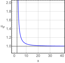
(a)

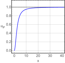
(b)

Figure 1: Group velocity of Eq. (42) for $\alpha>0$ LABEL:sub@caseNzero-positive-alpha and for $\alpha<0$ LABEL:sub@caseNzero-negative-alpha where $\vartheta=9\pi/10$. Asymptotes are illustrated as black, dotted lines.

First, the front velocity is given by $u_{\mathrm{fr}}=|\sin\vartheta|\leq 1$ independently from $\alpha$ and does not show any vicious behavior. Second, the group velocity reads

$${\mathbf{u}_{\mathrm{gr}}}=\frac{\mathbf{p}-\mathbf{\hat{\mathbf{B}}}(\mathbf{\hat{\mathbf{B}}}\cdot\mathbf{p})}{p_{0}}\,,$$ (41)

having a modulus given by

$$u_{\mathrm{gr}}=\frac{1}{\sqrt{1-\mathrm{sgn}(\alpha)[2x^{2}\sin^{2}\vartheta]^{-1}}}\,,\quad x=\eta|\mathbf{p}|\sqrt{|\alpha|}|\mathbf{B}|\,.$$ (42)

For $\alpha>0$, the velocity (42) is only well-defined for $\mathbf{p}^{2}>{(2\eta^{2}\alpha|\mathbf{B}|^{2}\sin^{2}{\vartheta})^{-1}}.$ One problem is that this minimum cut-off depends on the angle $\vartheta$, which is why it does not really work as a true cut-off. Besides, the mode does not behave like a standard photon for vanishing $\eta$. It is easy to notice that the group velocity is always larger than 1 and even singular for $\eta|\mathbf{p}||\mathbf{B}|=\csc{\vartheta}/\sqrt{2\alpha}$, i.e., the corresponding mode violates causality and is spurious. Its behavior is depicted in Fig. 1a as a function of $x$. In contrast, the group velocity for $\alpha<0$ does not exhibit any singularities. This mode is exotic, as its group velocity increases from zero and approaches the limit $u_{\mathrm{gr}}=1$ from below. A plot of its modulus is presented in Fig. 1b.

Another possibility worthwhile to consider is that of orthogonal $\mathbf{B}$ and $\mathbf{C}$, $\mathbf{B\cdot C}=0$. This configuration is especially interesting, because it implies $D_{ii}=0$ and Tr($D_{\mu\nu})=0$, whereupon it represents a higher-derivative electrodynamics that does not contain Podolsky’s sector at all. The dispersion equation (28) is

$$p^{4}(\eta^{4}{\mathbf{B}^{2}\mathbf{C}^{2}})+\eta^{4}p^{2}\left[{\mathbf{B}^{2}(\mathbf{C\cdot p})^{2}}+\mathbf{C}^{2}(\mathbf{B\cdot p})^{2}\right]-2\eta^{2}{(\mathbf{B\cdot p})}(\mathbf{C\cdot p})-1=0\,.$$ (43)

To analyze this situation, we adopt a coordinate system in which the vectors $\mathbf{C}$, $\mathbf{B}$ point along the $x$ and $y$ axis, respectively: $\mathbf{C}={|\mathbf{C}|}\mathbf{\hat{e}}_{x}$, $\mathbf{B}={|\mathbf{B}|}\mathbf{\hat{e}}_{y}$. The momentum $\mathbf{p}$ shall enclose an angle $\vartheta$ with the $z$ axis. In this system, it holds that

$$\mathbf{p}=\left|\mathbf{p}\right|\left(\sin\vartheta\cos\phi,\sin\vartheta\sin\phi,\cos\vartheta\right),$$ (44)

which implies ${\mathbf{B\cdot p}}=\left|\mathbf{B}\right|\left|\mathbf{p}\right|\sin\vartheta\cos\phi$ and ${\mathbf{C\cdot p}}=\left|\mathbf{C}\right|\left|\mathbf{p}\right|\sin\vartheta\sin\phi.$ The relation (43) is rewritten as

$${(p_{0}^{(\pm)})^{2}}=\alpha_{\vartheta}|\mathbf{p}|^{2}\pm{\frac{1}{\eta^{2}{|\mathbf{B}|}|\mathbf{C}|}\sqrt{\frac{1}{4}\nu_{1}^{2}|\mathbf{p}|^{4}+\nu_{1}|\mathbf{p}|^{2}\sin 2\phi+1}}\,,$$ (45a)

with

$$\alpha_{\vartheta}={1-\frac{1}{2}\sin^{2}\vartheta}\,,\quad\nu_{1}=\eta^{2}{|\mathbf{B}|}|\mathbf{C}|\sin^{2}\vartheta\,.$$ (45b)

In what follows, modes denoted by the glyph $\oplus$ will be identified with the upper sign choice of a dispersion relation, whereas modes called $\ominus$ will correspond to the lower one. The front velocity reads $u_{\mathrm{fr}}=1$ independently of the angles $\vartheta$ and $\phi$, which is a result compatible with causality. The next step is to evaluate the group velocity, whose modulus can be expressed in terms of the basis $\mathbf{B}={|\mathbf{B}|}\mathbf{\hat{e}}_{y},\mathbf{C}={|\mathbf{C}|}\mathbf{\hat{e}}_{x}$ by using the representation of the momentum of Eq. (44):

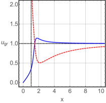
(a)

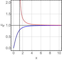
(b)

Figure 2: Group velocity of Eq. (46) for $\vartheta=3\pi/7$, $\phi=4\pi/5$ LABEL:sub@spacelike-case-orthogonal-vectors-1 and for $\vartheta=3\pi/4$, $\phi=2\pi/5$ LABEL:sub@spacelike-case-orthogonal-vectors-2. The group velocity for the mode $\oplus$ is represented by a plain, blue line, whereas the mode $\ominus$ is shown as a red, dashed line. Asymptotes are illustrated as black, dotted lines.

$${u_{\mathrm{gr}}^{(\pm)}}=\sqrt{\frac{4x^{2}\widetilde{\mathcal{S}}+2x^{4}\widetilde{\mathcal{T}}+x^{6}\widetilde{\mathcal{U}}}{Y^{2}\{x^{2}[3+\cos(2\vartheta)]\pm 2Y\}}}\,,$$ (46a)

with

$$\widetilde{\mathcal{S}} =3+\cos(2\vartheta)\pm Y\sin^{2}\vartheta\sin(2\phi)\,,$$ (46b)

$$\widetilde{\mathcal{T}} =2[3+\cos(2\vartheta)]\sin^{2}\vartheta\sin(2\phi)\pm Y\sin^{4}\vartheta\,,$$ (46c)

$$\widetilde{\mathcal{U}} =[3+\cos(2\vartheta)]\sin^{4}\vartheta\,,$$ (46d)

$$Y =\sqrt{4+x^{2}\sin^{2}\vartheta[x^{2}\sin^{2}\vartheta+4\sin(2\phi)]}\,,\quad x=\eta|\mathbf{p}|\sqrt{|\mathbf{B}||\mathbf{C}|}\,.$$ (46e)

The graph of Fig. 2 displays the modulus of the group velocity of the two modes $$\oplus \ominus \ominus x$$, considered in Eq. (46a) for different choices of the angles. Some comments are worthwhile. First, we point out that the group velocity of the mode diverges for the following choice of the dimensionless variable :

$$x_{\mathrm{sing}}=\frac{|\sec\vartheta|}{2}\sqrt{\sqrt{[3+\cos(2\vartheta)]^{2}-4\sin^{4}\vartheta\cos^{2}(2\phi)}+2\sin^{2}\vartheta\sin(2\phi)}\,.$$ (47)

This value is indicated by the dashed, vertical lines in Fig. 2. Because of the singularity, the behavior of the latter mode at momenta lying in this regime is unphysical. In contrast, the group velocity of the mode $\oplus$ (continuous line) does not have any singularities. For small momenta, the group velocities can be expanded as follows:

$${u_{\mathrm{gr}}^{(\pm)}}=\widetilde{\Theta}^{(\pm)}|\mathbf{p}|\,,\quad\widetilde{\Theta}^{(\pm)}=\eta\sqrt{|\mathbf{B}||\mathbf{C}|}\sqrt{\frac{1}{2}[\sin(2\phi)\mp 1]\sin^{2}\vartheta\pm 1}\,.$$ (48)

Each behaves like a Podolsky mode whose mass depends on the momentum direction. Note that such expansions can also be interpreted as expansions valid for a small controlling coefficient $\eta$. Furthermore, Fig. 2a shows that the group velocity of the mode $\oplus$ has a maximum, approaches 1 from above, and becomes larger than 1 (breaking causality) for a certain range of parameters. For the same values of the angles, the group velocity of the mode $\ominus$ decreases from its initial singularity to reach a minimum and finally approaches 1 from below. The graph 2b, generated for other values of the angles does not reveal any maxima or minima, with the group velocity of the mode $\ominus$ approaching 1 from above, and the mode $\oplus$ approaching 1 from below. For this parameter choice, the mode $\oplus$ is exotic. It was also verified that the mode $\ominus$ does not propagate for certain angles. For example, the group velocity vanishes identically for $\vartheta=\pi/2$ and $\phi=\pi/4$ where for $\vartheta=\pi/2$ and $\phi<[\pi+\arcsin(1/x^{2})]/2$ it even takes complex values.

So, we conclude that the spacelike configuration, $B_{\mu}=(0,\mathbf{B})_{\mu}$ and $C_{\mu}=(0,\mathbf{C})_{\mu}$, with parallel or orthogonal $\mathbf{B}$ and $\mathbf{C}$ can yield both exotic and spurious dispersion relations whose group velocities diverge or break causality. In general, such relations suggest meaningful signal propagation only in a regime of large momenta that is compatible with $u_{\mathrm{fr}}=1$. However, this interpretation is not capable of recovering a certain sector, once the dispersion relations associated cannot be considered as physical for a given momentum range.

III.2.5 Parity-odd anisotropic sector (with $\theta=0)$

A parity-odd anisotropic configuration is characterized by a purely timelike direction $C_{\mu}=(C_{0},0)_{\mu}$ and a purely spacelike one $B_{\mu}=(0,\mathbf{B})_{\mu}$, which leads to

$$p_{0}=\frac{\mathrm{sgn}(C_{0})\left|\mathbf{p}\right|\sqrt{\eta^{4}C_{0}^{2}|\mathbf{B}\times\mathbf{p}|^{4}+\mathbf{B}^{2}}-\mathbf{B\cdot p}}{\eta^{2}C_{0}|\mathbf{B}\times\mathbf{p}|^{2}}\,,$$ (49a)

or

$$p_{0}=\frac{\mathrm{sgn}(C_{0})\sqrt{1+\eta^{4}C_{0}^{2}\mathbf{B}^{2}\mathbf{p}^{4}\sin^{4}\vartheta_{B}}-\cos\vartheta_{B}}{\eta^{2}C_{0}|\mathbf{B}||\mathbf{p}|\sin^{2}\vartheta_{B}}\,,$$ (49b)

with ${\mathbf{B\cdot p}}=|\mathbf{B}||\mathbf{p}|\cos\vartheta_{B}$, $|\mathbf{B}\times\mathbf{p}|=|\mathbf{B}||\mathbf{p}|\sin\vartheta_{B}$. The dispersion relation is positive, real-valued, and not defined in the limit $C_{0}\mapsto 0$. The result for the front velocity is simply $u_{\mathrm{fr}}=1,$ not revealing any problems with causality in the large-momentum regime. The associated group velocity, however, is

$${u_{\mathrm{gr}}} =\left[(\eta|\mathbf{p}|)^{-4}C_{0}^{-2}\Upsilon^{-3}\left\{(\mathbf{B}\cdot\widehat{\mathbf{p}})\left[{\mathrm{sgn}(C_{0})}2\Xi(\Upsilon+4\mathbf{B}^{2})-4\mathbf{B}^{2}(\mathbf{B}\cdot\widehat{\mathbf{p}})\right]+2\mathbf{B}^{2}(\Upsilon-2\mathbf{B}^{2})-4\Xi^{2}\Upsilon\right\}\right.$$

$$\left.\phantom{{}={}}+5-4\Upsilon^{-1}\mathbf{B}^{2}\left[\mathrm{sgn}(C_{0})2\Xi^{-1}(\mathbf{B}\cdot\widehat{\mathbf{p}})-1\right]-4(\eta|\mathbf{p}|)^{4}\mathbf{B}^{2}C_{0}^{2}\Upsilon\Xi^{-2}\right]^{1/2}\,,$$ (50a)

with

$$\Upsilon=(\mathbf{B}\cdot\widehat{\mathbf{p}})^{2}-\mathbf{B}^{2}\,,\quad\Xi=\sqrt{\mathbf{B}^{2}+(\eta|\mathbf{p}|)^{4}C_{0}^{2}\Upsilon^{2}}\,.$$ (50b)

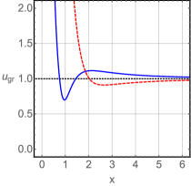
Figure 3: Group velocity of Eq. (III.2.5) for $\vartheta_{B}=3\pi/10$, $\mathrm{sgn}(C_{0})=1$ (blue, plain) and $\mathrm{sgn}(C_{0})=-1$ (red, dashed). The horizontal asymptote is illustrated as a black, dotted line.

Note that there is, in principle, a single mode only, i.e., the framework considered describes a nonbirefringent vacuum for photons. However, both the dispersion law and the group velocity depend on the sign of the component $C_{0}$ explicitly. In terms of the angle $\vartheta_{B}$ between $\mathbf{B}$ and $\mathbf{p}$, the result is expressed as

$$u_{\mathrm{gr}} =\left[1-4\csc^{2}\vartheta_{B}+{\mathrm{sgn}(C_{0})}\frac{8}{Y}\cot\vartheta_{B}\csc\vartheta_{B}+\frac{4x^{4}}{Y^{2}}\sin^{2}\vartheta_{B}\right.$$

$$\phantom{{}={}}\left.\,+\,\frac{1}{8{x^{4}}}\left\{\csc^{6}\left(\frac{\vartheta_{B}}{2}\right)(1-{\mathrm{sgn}(C_{0})}Y)+\sec^{6}\left(\frac{\vartheta_{B}}{2}\right)(1+{\mathrm{sgn}(C_{0})}Y)\right\}\right]^{1/2}\,,$$ (51)

where $Y=\sqrt{1+{(x\sin\vartheta)^{4}}}\,,$ $x={\eta|\mathbf{p}|\sqrt{|\mathbf{B}||C_{0}|}}\,.$ The group velocity becomes singular for a vanishing momentum only, see Fig. 3, which characterizes an unphysical regime for each sign of $C_{0}$, therefore. An expansion for a small momentum and controlling coefficient $\eta$, respectively, provides

$$u_{\mathrm{gr}}=\frac{1}{2\sqrt{2}x^{2}}\sqrt{[1+\mathrm{sgn}(C_{0})]\sec^{6}\left(\frac{\vartheta_{B}}{2}\right)+[1-\mathrm{sgn}(C_{0})]\csc^{6}\left(\frac{\vartheta_{B}}{2}\right)}\,,$$ (52)

explicitly revealing the singularities for both possible signs of $C_{0}$. Note that the group velocity of one of the modes (for $C_{0}<0$) has a minimum and approaches 1 from below for increasing $x$, whereas the group velocity of the second mode (for $C_{0}>0$) has both a minimum and a maximum and approaches 1 from above. The modulus of the group velocity becomes larger than 1 for both modes at some values of $x,$ which is a behavior that corresponds to causality violation. We also point out that the two modes merge into a single mode for $\vartheta=\pi/2,$ and that they interchange their role for $\vartheta\in(\pi/2,\pi]$. Both modes do not behave like standard photons when $\eta$ vanishes. As their group velocities exhibit singularities, they are spurious.

The compilation of the results obtained seems to reveal that this higher-derivative electrodynamics only exhibits well-behaved signal propagation in the limit of large momenta. But, the dispersion relations cannot be valid only for a given momentum range, unless a physically reasonable cutoff can be imposed on the theory. So, this interpretation will not be considered at this stage. For small momenta, some of the modes behave like a Podolsky mode where the Podolsky parameter can depend on the direction of the momentum due to anisotropy. We encountered exotic modes such as the dispersion relation $\oplus$ for the parameter choice used in Fig. 2b. The others that exhibit nonphysical features must be considered as spurious.

III.3 Unitarity analysis

At this point, we present some discussion on unitarity of this higher-derivative model. The analysis of unitarity at tree-level can be performed by means of a contraction of the propagator with external currents Veltman , which leads to a Lorentz scalar that is often referred to as the saturated propagator ($\mathit{SP}$):

$$\mathit{SP}\equiv J^{\mu}\Delta_{\mu\nu}J^{\nu}\,.$$ (53)

The gauge current $J^{\mu}$ is taken as real and satisfies the conservation law $\partial_{\mu}J^{\mu}=0$, which in momentum space reads $p_{\mu}J^{\mu}=0$. Therefore, a contraction with this current eliminates all contributions whose tensor structure contains at least a single four-momentum. The latter are associated with the gauge choice, i.e., these terms do not describe the physics of the system under consideration. In accordance with this method, unitarity is assured whenever the imaginary part of the residue of the saturation $SP$ evaluated at a vanishing denominator is positive.

We first assess the usual Podolsky theory, whose propagator is given by Eq. (24). Contractions with the external four-current provide

$$\mathit{SP}=-\mathrm{i}\left(\frac{J^{\nu}\Theta_{\nu\alpha}J^{\alpha}}{p^{2}\left(1-\theta^{2}p^{2}\right)}-\frac{\xi}{p^{2}}J^{\nu}\Omega_{\nu\alpha}J^{\alpha}\right)\,,$$ (54)

which simplifies to

$$\mathit{SP}=\frac{\mathrm{i}}{\theta^{2}}\left(\frac{J^{2}}{p^{2}\left(p^{2}-1/\theta^{2}\right)}\right)\,,$$ (55)

due to current conservation. As properly noted in Ref. Turcati , the latter can be written as

$$\mathit{SP}=\mathrm{i}\left(-\frac{J^{2}}{p^{2}}+\frac{J^{2}}{p^{2}-1/\theta^{2}}\right)\,.$$ (56)

For a physical spacelike current, $J^{2}<0,$ the pole $p^{2}=0$ yields a positive imaginary part of the residue of $\mathit{SP}$, while the pole $p^{2}=1/\theta^{2}$ provides a negative one, so that this theory reveals a nonunitary behavior associated with the massive mode. The Lee-Wick theories are plagued by the same problem, but mechanisms to recover unitarity by suppressing the negative-norm states are stated in the literature LWghost . Within this scenario, we point out that working with a Poldosky Lagrangian, whose term proportional to $\theta^{2}$ has a reversed sign, does not solve the unitarity problem at all (it only moves the problem from one pole to the other). Instead, it leads to a dispersion relation that is not well-defined for small enough momenta.

Considering the propagator of Eq. (25), defined in the absence of the Podolsky term ($\theta^{2}=0$), the saturation reads

$$\mathit{SP} =-\frac{\mathrm{i}}{p^{2}\Gamma(p)}\Big{\{}\Gamma(p)J^{2}-\,2\eta^{2}p^{2}(B\cdot J)(C\cdot J)\Pi_{\theta=0}(p)$$

$$\phantom{{}={}}\hskip 45.52458pt\left.+\,\eta^{4}p^{2}(B\cdot J)^{2}\left[(C\cdot p)^{2}-C^{2}p^{2}\right]+\eta^{4}p^{2}(C\cdot J)^{2}\left[(B\cdot p)^{2}-B^{2}p^{2}\right]\right\}\,,$$ (57)

with $\Pi_{\theta=0}(p)$ given by Eq. (26). The latter should be analysed with respect to the residue of each denominator.

• First pole: The residue of the saturation evaluated at $p^{2}=0$ is simply given by

  $$\mathrm{Res}(\textit{SP})|_{p^{2}=0}=-\mathrm{i}J^{2}\,.$$ (58)

  A spacelike $J^{2}<0$ yields $\mathrm{Im}[\mathrm{Res}(\textit{SP})|_{p^{2}=0}]>0$, which is why unitarity is assured. Therefore, we deduce that a quantization of this mode, which is the standard one of electrodynamics, corresponds to the photon.

• Second pole: Evaluating the residue at $\Gamma(p)=0$ works in the same manner, in principle:

  $$\mathrm{Res}(\mathit{SP})|_{\Gamma(p)=0} =-\mathrm{i}\eta^{2}\Big{\{}\eta^{2}(B\cdot J)^{2}\left[(C\cdot p)^{2}-C^{2}p^{2}\right]+\eta^{2}(C\cdot J)^{2}\left[(B\cdot p)^{2}-B^{2}p^{2}\right]$$

  $$\phantom{{}={}}\hskip 28.45274pt-2(B\cdot J)(C\cdot J)\Pi_{\theta=0}(p)\Big{\}}\Big{|}_{\Gamma(p)=0}\,.$$ (59)

  The situation now is more involved, and requires a careful analysis to find the global sign of the expression in curly brackets. Considering Eq. (23a), an evaluation of $\Gamma(p)=0$ provides the useful relationship

  $$\mathrm{sgn}(\Pi_{\theta=0})\Pi(p)|_{\begin{subarray}{c}\theta=0\\ \Gamma(p)=0\end{subarray}}=\eta^{2}\sqrt{\left[(B\cdot p)^{2}-B^{2}p^{2}\right]\left[(C\cdot p)^{2}-C^{2}p^{2}\right]}\big{|}_{\Gamma(p)=0}\,.$$ (60)

  The sign function on the left-hand side must be taken into account, as $\Pi_{\theta=0}(p)$ can be a negative quantity onshell, whereas the right-hand side is manifestly positive. Furthermore, we again have to distinguish between two cases. After investigating a large number of Lorentz-violating sectors numerically, we deduced that either $p^{\mu}\in M_{1}$ or $p^{\mu}\in M_{2}$ with the two sets $M_{1}\equiv\{(B\cdot p)^{2}-B^{2}p^{2}>0,(C\cdot p)^{2}-C^{2}p^{2}>0\}$ or $M_{2}\equiv\{(B\cdot p)^{2}-B^{2}p^{2}<0,(C\cdot p)^{2}-C^{2}p^{2}<0\}$. Both options assure a real $\Pi(p).$ For the first option, the residue can be expressed in terms of the square of a sum of two terms. For the second option, a global minus sign must be pulled out of the whole expression, reversing the global saturation sign. The residues can then neatly be written as follows:

  $$\mathrm{Res}(\mathit{SP})|_{\Gamma(p)=0}=\mathrm{i}\eta^{4}\left\{\begin{array}[]{lcl}-\Big{\{}(B\cdot J)\sqrt{(C\cdot p)^{2}-C^{2}p^{2}}&\text{for}&p^{\mu}\in M_{1}\,,\\ \phantom{{}}-\mathrm{sgn}(\Pi_{\theta=0})(C\cdot J)\sqrt{(B\cdot p)^{2}-B^{2}p^{2}}\Big{\}}^{2}\Big{|}_{\Gamma(p)=0}&&\\ \Big{\{}(B\cdot J)\sqrt{|(C\cdot p)^{2}-C^{2}p^{2}|}&\text{for}&p^{\mu}\in M_{2}\,.\\ \phantom{{}}+\mathrm{sgn}(\Pi_{\theta=0})(C\cdot J)\sqrt{|(B\cdot p)^{2}-B^{2}p^{2}|}\Big{\}}^{2}\Big{|}_{\Gamma(p)=0}&&\\ \end{array}\right.$$ (61)

Hence, $\mathrm{Im}[\mathrm{Res}(\mathit{SP})|_{\Gamma(p)=0}]<0$ for the first case, which is a behavior indicating a breakdown of unitarity. The second case behaves in the opposite way, whereupon unitarity is preserved. The parity-odd configuration with $(C_{\mu})=(C_{0},\mathbf{0})$, $(B_{\mu})=(0,\mathbf{B})$ analysed in Sec. III.2.4 is covered by the latter case. We find

$$(B\cdot p)^{2}-B^{2}p^{2}=-\frac{|\mathbf{B}|}{2\eta^{2}|\mathbf{C}|}<0\,,\quad(C\cdot p)^{2}-C^{2}p^{2}=-\frac{|\mathbf{C}|}{2\eta^{2}|\mathbf{B}|}<0\,,$$ (62)

which is why $p^{\mu}\in M_{2}$ in this sector. Thus, unitarity is preserved for this configuration.

For the parity-odd case introduced in Sec. III.2.5 it holds that $(C\cdot p)^{2}-C^{2}p^{2}=C_{0}^{2}\mathbf{p}^{2}>0$. However, it is a bit more involved to evaluate the second condition. The inequality $(B\cdot p)^{2}-B^{2}p^{2}\geq 0$ to be checked can be cast into a more transparent form as follows:

$$2x^{4}\sin^{4}\vartheta_{B}\cos^{2}\vartheta_{B}+\left\{3+\cos(2\vartheta_{B})-4\,\mathrm{sgn}(C_{0})\cos(\vartheta_{B})\sqrt{1+x^{4}\sin^{4}\vartheta_{B}}\right\}\geq 0\,,$$ (63a)

which is equivalent to

$$2\left\{1-\mathrm{sgn}(C_{0})\cos\vartheta_{B}\sqrt{1+x^{4}\sin^{4}\vartheta_{B}}\right\}^{2}\geq 0\,.$$ (63b)

The latter involves the angle $\vartheta_{B}$ defined directly below Eq. (49b) and the dimensionless quantity $x$ defined under Eq. (III.2.5). For $C_{0}>0$, the equality sign is valid for $\vartheta_{B}=0$ only, whereas for $C_{0}<0$ it is valid for $\vartheta_{B}=\pi$. Apart from these very special values at the boundaries of the interval for $\vartheta_{B}$, the condition $(B\cdot p)^{2}-B^{2}p^{2}>0$ is fulfilled manifestly, whereby $p^{\mu}\in M_{1}$. Therefore, according to our criterion, there are issues with unitarity for this sector.

There is an alternative possibility of calculating the saturated propagator. Using the transverse (T) and longitudinal (L) projection operators $\Theta_{\mu\nu}$ and $\Omega_{\mu\nu}$ of Eq. (13) transformed to momentum space, the propagator can be decomposed into the four parts $\Delta^{TT}_{\mu\nu}\equiv\Theta_{\mu\alpha}\Delta^{\alpha\beta}\Theta_{\beta\nu}$, $\Delta^{TL}_{\mu\nu}\equiv\Theta_{\mu\alpha}\Delta^{\alpha\beta}\Omega_{\beta\nu}$, $\Delta^{LT}_{\mu\nu}\equiv\Omega_{\mu\alpha}\Delta^{\alpha\beta}\Theta_{\beta\nu}$, and $\Delta^{LL}_{\mu\nu}\equiv\Omega_{\mu\alpha}\Delta^{\alpha\beta}\Omega_{\beta\nu}$. After performing contractions with the conserved current, only $\Delta^{TT}_{\mu\nu}$ will survive. Following this procedure, the saturated propagator can be cast into the form

SP $$=J^{\mu}\Delta^{TT}_{\mu\nu}J^{\nu}\,,\quad\Delta^{TT}_{\mu\nu}=-\mathrm{i}\frac{(M^{-1})_{\mu\nu}}{p^{2}}\,,$$ (64a)

$$M^{\mu\nu} =\left[(1-\theta^{2}p^{2})g-2\eta^{2}D^{TT}p^{2}\right]^{\mu\nu}\,,\quad(D^{TT})_{\mu\nu}\equiv\Theta_{\mu\alpha}D^{\alpha\beta}\Theta_{\beta\nu}\,.$$ (64b)

Hence, the behavior of unitarity is completely controlled by the totally transverse part of the matrix $D_{\mu\nu}$. Performing a formal partial-fraction decomposition, the standard pole $p^{2}=0$ can be separated from the remaining expressions involving the Podolsky parameter and the Lorentz-violating coefficient:

$$\Delta_{\mu\nu}^{TT}=-\mathrm{i}\left\{\frac{g_{\mu\nu}}{p^{2}}+(\theta^{2}\delta+2\eta^{2}D^{TT})_{\mu}^{\phantom{\mu}\alpha}(M^{-1})_{\alpha\nu}\right\}\,.$$ (65)

Using the explicit decomposition of $D_{\mu\nu}$ in terms of two four-vectors proposed in Eq. (14) and setting $\theta=0$, we can deduce that $\det(M)=\Gamma(p)$ with $\Gamma(p)$ from Eq. (60) for $\theta=0$. The result of Eq. (65) is suitable to investigate unitarity for the case of a nonzero $\theta$ and a general $D_{\mu\nu}$ whose form does not rely on a decomposition into two four-vectors. The analysis of such cases is an interesting open problem.

To conclude this section, unitarity violation seems to be connected to the appearance of additional time derivatives in the Lorentz-violating contributions of the Lagrange density, cf. Eqs. (11), (12). A behavior of this kind is expected. For a Lorentz-invariant, higher-derivative theory it was observed in LeeWick , amongst other works. The authors of Colladay:2001wk pointed out that additional time derivatives in the minimal SME fermion sector lead to issues with the time evolution of asymptotic states. Related problems in the nonminimal SME were found in the third and second paper of Kostelec1 and Kostelec2 , respectively.

IV Generalized model involving anisotropic Podolsky and Lee-Wick terms

There are two other CPT-even dimension-6 terms endowed with two additional derivatives, besides the LV modification (2), that can be expressed in terms of the electromagnetic field strength tensor and the tensor $D^{\mu\nu},$ namely:

$${D^{\alpha\beta}}F_{\mu\nu}\partial_{\alpha}\partial_{\beta}F^{\mu}{}^{\nu}\,,\quad{D^{\mu\nu}}\partial_{\sigma}F^{\sigma\lambda}{}\partial_{\mu}F_{\nu\lambda}\,.$$ (66)

The first one is a kind of anisotropic Lee-Wick term, while the second yields a bilinear contribution similar to it, but with the opposite sign, so that only one of these terms will be considered. The very same correspondence observed for the case of the anisotropic Podolsky term holds for the anisotropic Lee-Wick term, too: for the configuration of a diagonal tensor $D_{\beta\alpha}$ of the form $D_{\beta\alpha}=D_{00}g_{\beta\alpha}$, it becomes proportional to the usual Lee-Wick term, that is,

$${D^{\alpha\beta}}F_{\mu\nu}\partial_{\alpha}\partial_{\beta}F^{\mu\nu}=D_{00}(F_{\mu\nu}\square F^{\mu\nu})\,.$$ (67)

The behavior of the coefficients of the tensor $D_{\beta\alpha}$ under discrete C, P, and T operations, described in Tab. 1, does not depend on the way how the tensor is coupled to the electromagnetic field, being equally valid for the anisotropic Lee-Wick structures of Eq. (66).

In principle, the most general LV dimension-6 electrodynamics, modified by a rank-2 symmetric tensor, $D_{\beta\alpha},$ also includes the second of the anisotropic Lee-Wick contributions of Eq. (66), and is represented by the following Lagrangian:

$$\mathcal{L}=-\frac{1}{4}F_{\mu\nu}F^{\mu}{}^{\nu}+\frac{\theta^{2}}{2}\partial_{\alpha}F^{\alpha}{}^{\beta}\partial_{\lambda}F_{\phantom{\lambda}\beta}^{\lambda}+\eta_{1}^{2}D_{\beta\alpha}\partial_{\sigma}F^{\sigma}{}^{\beta}\partial_{\lambda}F^{\lambda\alpha}+\eta_{2}^{2}D^{\beta\alpha}\partial_{\sigma}F^{\sigma}{}^{\lambda}\partial_{\beta}F_{\alpha\lambda}+\frac{1}{2\xi}(\partial_{\mu}A^{\mu})^{2}\,,$$ (68)

with $\theta\geq 0$, $\eta_{1}\geq 0$, and $\eta_{2}\geq 0$. The latter incorporates the standard Podolsky term, its LV modification considered earlier, and the LV anisotropic Lee-Wick contribution. Such a Lagrangian can be written in the form $\mathcal{L}=(1/2)A^{\mu}\bar{O}_{\mu\nu}A^{\nu}$ where

$$\bar{O}_{\mu\nu} =(1+\theta^{2}\square+2\eta_{2}^{2}{D^{\beta\alpha}}\partial_{\beta}\partial_{\alpha})\square\Theta_{\mu\nu}+\left(2\eta_{1}^{2}D^{\beta\alpha}\partial_{\beta}\partial_{\alpha}-\frac{1}{\xi}\right)\square\Omega_{\mu\nu}+2\eta_{1}^{2}{D_{\nu\mu}}\square^{2}$$

$$\phantom{{}={}}-2\eta_{1}^{2}{D_{\nu\alpha}}\square\partial_{\mu}\partial^{\alpha}-2\eta_{1}^{2}{D_{\sigma\mu}}\square\partial_{\nu}\partial^{\sigma}\,.$$ (69)

Based on the prescription (14) for the symmetric tensor $D_{\beta\alpha}$ we obtain

$$\bar{O}_{\mu\nu} =(1+\theta^{2}\square+2\eta_{2}^{2}{\kappa\rho})\square\Theta_{\mu\nu}+\left(2\eta_{1}^{2}{\kappa\rho}-\frac{1}{\xi}\right)\square\Omega_{\mu\nu}+\eta_{1}^{2}{(B_{\mu}C_{\nu}+B_{\nu}C_{\mu})}\square^{2}$$

$$\phantom{{}={}}-\eta_{1}^{2}{(C_{\nu}\partial_{\mu}+C_{\mu}\partial_{\nu})\kappa}\square-\eta_{1}^{2}{(\partial_{\nu}B_{\mu}+\partial_{\mu}B_{\nu})\rho}\square\,,$$ (70)

with $\kappa$ and $\rho$ of Eq. (16). Using the same tensor algebra as that of the first case, the following propagator can be derived:

$$\Delta_{\nu\alpha} =-\frac{\mathrm{i}}{p^{2}\Delta(p)}\left\{\tilde{\Gamma}(p)\Theta_{\nu\alpha}+\left[b^{\prime}-\xi\Delta(p)\right]\Omega_{\nu\alpha}\right.$$

$$\phantom{{}={}-\mathrm{i}p^{2}\Delta(p)}\left.-\,\mathrm{i}\tilde{F}(p)(B_{\nu}p_{\alpha}+B_{\alpha}p_{\nu})-2\eta_{1}^{2}D_{\nu\alpha}p^{2}\tilde{\Pi}(p)-\mathrm{i}\tilde{H}(p)(C_{\nu}p_{\alpha}+C_{\alpha}p_{\nu})\right.$$

$$\phantom{{}={}-\mathrm{i}p^{2}\Delta(p)}\left.+\,\eta_{1}^{4}B_{\nu}B_{\alpha}\left[(C\cdot p)^{2}-C^{2}p^{2}\right]p^{2}+\eta_{1}^{4}C_{\nu}C_{\alpha}\left[(B\cdot p)^{2}-B^{2}p^{2}\right]p^{2}\right\}\,,$$ (71a)

where

$$\Delta(p) =[1-\theta^{2}p^{2}-2\eta_{2}^{2}(B\cdot p)(C\cdot p)]\tilde{\Gamma}(p)\,,$$ (71b)

$$\tilde{\Gamma}(p) =\eta_{1}^{4}\left[(B\cdot p)^{2}-B^{2}p^{2}\right]\left[(C\cdot p)^{2}-C^{2}p^{2}\right]-\tilde{\Pi}^{2}(p)\,,$$ (71c)

$$\tilde{\Pi}(p) =1-\theta^{2}p^{2}-\eta_{1}^{2}p^{2}(B\cdot C)+[\eta_{1}^{2}-2\eta_{2}^{2}](B\cdot p)(C\cdot p)\,,$$ (71d)

$$\tilde{F}(p) =F(p)|_{\eta=\eta_{1}}\,,\quad\tilde{H}(p)=H(p)|_{\eta=\eta_{1}}\,,$$ (71e)

with $F(p)$ and $H(p)$ of Eqs. (22b) and (22c), respectively. The new dispersion equations read

$$0 =p^{2}[1-\theta^{2}p^{2}-2\eta_{2}^{2}(B\cdot p)(C\cdot p)]\,,$$ (72a)

$$0 =\tilde{\Gamma}(p)\,.$$ (72b)

We now observe that in contrast to Eq. (27a), Podolsky’s dispersion relation is also modified, as shown in Eq. (72a).

IV.1 Dispersion relations

To analyse the dispersion equations (72a) and (72b), we consider the main two background configurations – timelike and spacelike – discussed in the first model. The Podolsky parameter $\theta$ will not be discarded.

IV.1.1 Timelike isotropic sector (with $\theta\neq 0)$

The timelike isotropic configuration is characterized by $B_{\mu}=(B_{0},\mathbf{0})_{\mu}$, $C_{\mu}=(C_{0},\mathbf{0})_{\mu}$. As already mentioned, the dispersion equation (72a) shows that the usual Podolsky dispersion relation is now modified by a contribution resulting from the anisotropic Lee-Wick term. In this case, the dispersion relation obtained from Eq. (72a) takes the simple form,

$$p_{0}=\sqrt{\frac{1}{\varepsilon}\left(\mathbf{p}^{2}+\frac{1}{\theta^{2}}\right)}\,,$$ (73)

with $\varepsilon=1+2\eta_{2}^{2}B_{0}C_{0}/\theta^{2}$. The latter is a Podolsky-like dispersion relation, modified by a kind of dielectric constant, $\varepsilon$. For $B_{0}C_{0}>0$, the front velocity is less than one, $u_{\mathrm{fr}}<1,$ and the group velocity,

$$u_{\mathrm{gr}}=\frac{|\mathbf{p}|}{\sqrt{\varepsilon}\sqrt{\mathbf{p}^{2}+1/\theta^{2}}}\,,$$ (74)

is always less than 1, as well, ensuring the validity of causality for this configuration. The DR (73) only makes sense in the presence of the Podolsky term ($\theta^{2}\neq 0)$. Note that $\theta^{2}$ appears inside $\varepsilon$, as well. Now, we analyse the dispersion equation (72b) for the isotropic configuration with $B_{\mu}=(B_{0},\mathbf{0})_{\mu}$, $C_{\mu}=(C_{0},\mathbf{0})_{\mu}$, which can be written as

$$E^{(\pm)}=\psi^{(\pm)}|\mathbf{p}|\,,\quad\psi^{(\pm)}=\psi^{(\pm)}(|\mathbf{p}|)\,,$$ (75a)

where

$$\psi^{(+)} =\sqrt{\frac{1+\theta^{2}|\mathbf{p}|^{2}}{2y^{2}+\theta^{2}|\mathbf{p}|^{2}}}\,,$$ (75b)

$$\psi^{(-)} =\sqrt{\frac{1+2x^{2}+\theta^{2}|\mathbf{p}|^{2}}{2y^{2}+\theta^{2}|\mathbf{p}|^{2}}}\,,$$ (75c)

and $$x=\sqrt{B_{0}C_{0}}\eta_{1}|\mathbf{p}| y=\sqrt{B_{0}C_{0}}\eta_{2}|\mathbf{p}| x y x/(\theta|\mathbf{p}|)=\sqrt{B_{0}C_{0}}\eta_{1}/\theta\equiv\alpha y/(\theta|\mathbf{p}|)=\sqrt{|\mathbf{B}||\mathbf{C}|}\eta_{2}/\theta\equiv\beta x \alpha\theta|\mathbf{p}| y \beta\theta|\mathbf{p}|$$, are dimensionless coefficients. Note that both and are linear functions of the three-momentum magnitude where the ratios and are dimensionless. Hence, it is reasonable to investigate the expressions for the characteristic velocities after replacing by and by , respectively. Now, the front velocities for both modes are simply given by

$$u_{\mathrm{fr}}^{(+)} =\frac{1}{\sqrt{1+2\beta^{2}}}\,,$$ (76a)

$$u_{\mathrm{fr}}^{(-)} =\sqrt{\frac{1+2\alpha^{2}}{1+2\beta^{2}}}\,.$$ (76b)

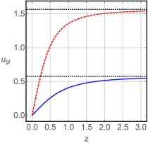
(a)

Figure 4: Group velocities of Eq. (77) as a function of $z=\theta|\mathbf{p}|$ for the mode $\oplus$ (blue, plain) with $\beta=1$ and for $\ominus$ with $\alpha=1$, $\beta=1/3$ (red, dashed). The horizontal asymptotes are shown as black, dotted lines.

The first of these expressions is always smaller than 1, whereas the second can be larger than 1 for $\alpha>\beta$. As the case under consideration is isotropic, it is not too involved to obtain the group velocities:

$$u_{\mathrm{gr}}^{(+)} =\frac{\psi^{(+)}}{1+(\theta|\mathbf{p}|)^{-2}}\,,$$ (77a)

$$u_{\mathrm{gr}}^{(-)} =\psi^{(-)}\left\{1-\frac{1}{(\psi^{(-)})^{2}\left[2y^{2}+(\theta|\mathbf{p}|)^{2}\right]}\right\}\,.$$ (77b)

Both expressions do not exhibit any singularities. The graph of Fig. 4 reveals decreasing group velocities for declining momenta where each mode behaves as a Podolsky mode in this regime:

$$u_{\mathrm{gr}}^{(\pm)} =\widehat{\Theta}^{(\pm)}|\mathbf{p}|\,,$$ (78a)

$$\widehat{\Theta}^{(+)} =\frac{\theta}{\sqrt{1+2\beta^{2}}}\,,\quad\widehat{\Theta}^{(-)}=\frac{(1+2\alpha^{2})\theta}{\sqrt{1+2\beta^{2}}}\,.$$ (78b)

As the case under consideration is isotropic, the Podolsky parameters do not depend on the momentum direction, but they involve the Lorentz-violating coefficients. Causality violation can occur for the mode $\ominus$ dependent on the chosen parameters. The group velocity for each mode rises from 0 to a finite value that is given by the previously obtained expressions for the front velocity:

$$\lim_{z\mapsto\infty}u_{\mathrm{gr}}^{(+)}=u_{\mathrm{fr}}^{(+)}\,,\quad\lim_{z\mapsto\infty}u_{\mathrm{gr}}^{(-)}=u_{\mathrm{fr}}^{(-)}\,.$$ (79)

Hence, the group velocity of the mode $\ominus$ can reach values larger than 1, breaking causality, which characterizes a spurious mode. On the other hand, the mode $\oplus$ mode does not violate causality, although it does not behave like a standard photon for vanishing $\eta_{1}$ or $\eta_{2}$. So it is an exotic mode. Note that vanishing Lorentz violation translates into the limits $\alpha\mapsto 0$ and $\beta\mapsto 0$, which provides the Podolsky-type dispersion law.

IV.1.2 Parity-even anisotropic sector (with $\theta\neq 0)$

For the spatially anisotropic configuration, $B_{\mu}=(0,\mathbf{B})_{\mu}$, $C_{\mu}=(0,\mathbf{C})_{\mu}$, we can express the dispersion relation following from Eq. (72a) as follows:

$$p_{0}^{2}=\frac{1}{\theta^{2}}+\mathbf{p}^{2}-{\frac{2\eta_{2}^{2}}{\theta^{2}}}(\mathbf{B\cdot p})(\mathbf{C\cdot p})\,,$$ (80)

which for $\eta_{2}\mapsto 0$ recovers Podolsky’s dispersion relation. To analyze the dispersion relation for $\eta_{2}\neq 0$, we first consider the situation in which the vectors $\mathbf{C}$, $\mathbf{B}$ are orthogonal. Using the coordinate system employed in Sec. III.2.4 with the momentum of Eq. (44), implies

$$p_{0}=\sqrt{\frac{1}{\theta^{2}}+\mathbf{p}^{2}\left(1-\frac{\eta_{2}^{2}}{\theta^{2}}|\mathbf{B}||\mathbf{C}|\sin^{2}\vartheta\sin 2\phi\right)}\,.$$ (81)

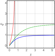
Figure 5: Group velocity of Eq. (83) for $\beta=1$, $\vartheta=\phi=0$ (blue, plain), for $\beta=3/2$, $\vartheta=\pi/5$, $\phi=\pi/3$ (green, dash-dotted), and for $\beta=2$, $\vartheta=\pi/2$, $\phi=\pi/3$ (red, dashed). The asymptotes are indicated by black, dotted lines.

Here, the front velocity is

$$u_{\mathrm{fr}}=\sqrt{1-{\frac{\eta_{2}^{2}}{\theta^{2}}|\mathbf{B}||\mathbf{C}|}\sin^{2}\vartheta\sin(2\phi)}\,,$$ (82)

which can be larger than 1 for some values of $\phi.$ The modulus of the group velocity is given by

$${u_{\mathrm{gr}}=\sqrt{2+\frac{y^{4}\sin^{2}\vartheta-z^{2}(2+z^{2})}{z^{2}\left[1+z^{2}-y^{2}\sin^{2}\vartheta\sin(2\phi)\right]}}}\,,$$ (83)

with $y=\sqrt{|\mathbf{B}||\mathbf{C}|}\eta_{2}|\mathbf{p}|$, $z=\theta|\mathbf{p}|$. Here we introduce the constant ratio $y/z=\sqrt{|\mathbf{B}||\mathbf{C}|}\eta_{2}/\theta\equiv\beta$. The graph of Fig. 5 shows the behavior of the group velocity for distinct values of the parameter $\beta$ and the angles. The latter $\beta$ can be chosen such that $u_{\mathrm{gr}}$ rises steadily from 0 and approaches a certain constant from below for increasing $z$. Explicitly, this constant exceeds 1 at

$$z|_{u_{\mathrm{gr}}=1}=\frac{\csc\vartheta}{|\beta|\sqrt{\beta^{2}-\sin(2\phi)}}\,,$$ (84)

whereupon there will be issues with causality. This value of $z$ is real for $\beta>\sqrt{\sin(2\phi)}$ only, which demonstrates that causality problems do not arise necessarily. Besides, $u_{\mathrm{gr}}$ also exhibits a singularity for a suitable choice of the parameters that lies at the value

$$z_{\mathrm{sing}}=\frac{1}{\beta^{2}\sin^{2}\vartheta\sin(2\phi)-1}\,,$$ (85)

revealing an unphysical regime. For small momenta, the group velocity of Eq. (83) behaves as

$$u_{\mathrm{gr}}=\breve{\Theta}|\mathbf{p}|\,,\quad\breve{\Theta}=\theta\sqrt{1+\beta^{2}[\beta^{2}-2\sin(2\phi)]\sin^{2}\vartheta}\,,$$ (86)

so the corresponding mode propagates as a Podolsky-type mode with a modified mass depending on the momentum direction. Note the similarities to Eq. (48). The limit $\beta\mapsto 0$ for vanishing Lorentz violation reproduces the behavior of the conventional Podolsky mode.

For this spacelike configuration, we now investigate the dispersion relation derived from Eq. (72b) by initially studying the case of orthogonal vectors $\mathbf{B}$, $\mathbf{C}$. This configuration yields two different additional dispersion relations, written as

$$(p_{0}^{(\pm)})^{2}=\frac{\mathbf{p}^{2}}{z^{4}-x^{4}}\left\{\mathcal{V}/2\pm\sqrt{(z^{4}-x^{4}){\left[x^{4}\cos^{2}\vartheta-\mathcal{W}\right]}+(\mathcal{V}/2)^{2}}\right\}\,,$$ (87a)

where

$$\mathcal{V} =2z^{2}(1+z^{2})-2x^{4}+\sin^{2}\vartheta\left[x^{2}+(x^{2}-2y^{2})z^{2}\sin(2\phi)\right]\,,$$ (87b)

$$\mathcal{W} =\left[1+z^{2}-y^{2}\sin^{2}\vartheta\sin(2\phi)\right]\left[1+z^{2}+(x^{2}-y^{2})\sin^{2}\vartheta\sin(2\phi)\right]\,,$$ (87c)

and

$$x=\sqrt{|\mathbf{B}||\mathbf{C}|}\eta_{1}|\mathbf{p}|\,,\quad y=\sqrt{|\mathbf{B}||\mathbf{C}|}\eta_{2}|\mathbf{p}|\,,\quad z=\theta|\mathbf{p}|\,.$$ (87d)

The modulus squared of the group velocity is given by a highly involved expression

$$(u_{\mathrm{gr}}^{(\pm)})^{2}=\frac{|\mathbf{p}|^{2}}{(p_{0}^{(\pm)})^{2}}\left(\cos^{2}\vartheta+\frac{{f_{\pm}^{2}}(\vartheta,\phi)+{f_{\pm}^{2}}(\vartheta,\pi/2-\phi)}{{g_{\pm}^{2}}(\vartheta,\phi)}\right)\,,$$ (88a)

with

$$f_{\pm}(\vartheta,\phi) =2y^{2}(y^{2}-x^{2})\sin^{3}\vartheta\sin(2\phi)\sin\phi$$

$$\phantom{{}={}}+(x^{2}-2y^{2})\left\{1+z^{2}\left[2\sin^{2}\vartheta\cos^{2}\phi+1-(e^{(\pm)})^{2}\right]\right\}\sin\vartheta\sin\phi$$

$$\phantom{{}={}}+\left(x^{4}\left[(e^{(\pm)})^{2}-\cos^{2}\vartheta\right]+2z^{2}\left\{1+\left[1-(e^{(\pm)})^{2}\right]z^{2}\right\}\right)\sin\vartheta\cos\phi\,,$$ (88b)

$$g_{\pm}(\vartheta,\phi) =\left[2(e^{(\pm)})^{2}-1-\cos^{2}\vartheta\right]x^{4}+\left[2+(x^{2}-2y^{2})\sin^{2}\vartheta\sin(2\phi)\right]z^{2}$$

$$\phantom{{}={}}+2\left[1-(e^{(\pm)})^{2}\right]z^{4}\,,$$ (88c)

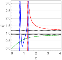
(a)

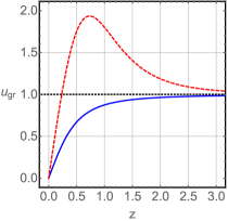
(b)

Figure 6: Group velocity of Eq. (88) of the mode $\oplus$ for the parameters $\alpha=3/2$, $\beta=2$, $\vartheta=\pi/2$, $\phi=\pi/3$ (blue, plain), for $\alpha=3/2$, $\beta=1$, $\vartheta=\pi/4$, $\phi=0$ (red, dotted), and for $\alpha=1/3$, $\beta=1/2$, $\vartheta=\pi/2$, $\phi=\pi/4$ (green, dash-dotted) LABEL:sub@fig:full-spacelike-orthogonal-case-1. The group velocity of the mode $\ominus$ for $\alpha=3/2$, $\beta=1$, $\vartheta=0$, $\phi=0$ (blue, plain) and for $\alpha=3/2$, $\beta=3$, $\vartheta=\pi/2$, $\phi=0$ (red, dotted) is shown in LABEL:sub@fig:full-spacelike-orthogonal-case-2. Vertical asymptotes at singularities are illustrated via color-coded, dotted lines, whereas horizontal asymptotes are shown as black, dotted lines.

where $e^{(\pm)}\equiv p_{0}^{(\pm)}/|\mathbf{p}|$. Fig. 6 shows the group velocity for the modes $\oplus$ and $\ominus$ for different angles and parameters $\sqrt{|\mathbf{B}||\mathbf{C}|}\eta_{1}/\theta\equiv\alpha$ and $\sqrt{|\mathbf{B}||\mathbf{C}|}\eta_{2}/\theta\equiv\beta$. The group velocity of the mode $\oplus$ is badly behaved for a broad range of parameters and angles, as it exhibits one or even two singularities that lie at the following values of $z$:

$$z_{\mathrm{sing}}^{(\pm)}=\frac{\sqrt{2}}{\sqrt{(2\beta^{2}-\alpha^{2})\sin^{2}\vartheta\sin(2\phi)-2\pm\alpha^{2}\sqrt{4\cos^{2}\vartheta+\sin^{4}\vartheta\sin^{2}(2\phi)}}}\,.$$ (89)

Besides, when there are singularities, the group velocity even becomes complex for large domains of the momentum. For small momenta, the group velocity for both modes exhibits the following asymptotic behavior:

$$u_{\mathrm{gr}}^{(\pm)} =\bar{\Theta}^{(\pm)}|\mathbf{p}|\,,$$ (90a)

$$\bar{\Theta}^{(\pm)} =\theta\sqrt{1\mp\alpha^{2}+\frac{\sin^{2}\vartheta\left[\alpha^{2}(\pm\alpha^{2}-2)\pm 2\beta^{2}(\alpha^{2}-\beta^{2})+(\alpha^{2}\mp 2)(\alpha^{2}-2\beta^{2})\sin(2\phi)\right]}{2(\alpha^{2}\mp 1)}}\,.$$ (90b)

Hence, these modes are modifications of the Podolsky mode with anisotropic Podolsky parameters that can become complex when the parameters are chosen suitably. The Podolsky mode is reproduced in the combined limit $\alpha\mapsto 0$ and $\beta\mapsto 0$. For certain choices, the group velocity is well-behaved in the sense that it increases monotonically from $0$ until it approaches a value smaller than 1 from below, cf. the green curve in Fig. 6a. It then behaves like an exotic mode. The other curves in this figure correspond to parameter choices that provide spurious behaviors. In contrast, the mode $\ominus$ in Fig. 6b does not exhibit any singularities. It rises from 0 and converges to a value smaller then 1 from below or larger than 1 from above. The latter behavior, though, is interpreted as a violation of causality, which occurs at least for some parameter choices. Therefore, the mode represented by the blue curve is exotic, whereas the mode illustrated by the red curve is spurious.

We can also present expansions for the front velocities following from DR (87a) in the limit of a large Podolsky parameter $\theta$ in comparison to the LV coefficients $\eta_{1}$, $\eta_{2}$:

$$u_{\mathrm{fr}}^{(+)} \approx 1+\frac{1}{2}\left[\left(\frac{x}{z}\right)^{2}-\left(\frac{y}{z}\right)^{2}\right]\sin^{2}\vartheta\sin(2\phi)\,,$$ (91a)

$$u_{\mathrm{fr}}^{(-)} \approx 1-\frac{1}{2}\left(\frac{y}{z}\right)^{2}\sin^{2}\vartheta\sin(2\phi)\,.$$ (91b)

Both can be larger than 1, depending on the relative sizes of $$x y \phi, \oplus \ominus$$, and on the angle which spoils the premises of causality. Thus, while the mode is unphysical in several senses, the mode breaks causality for certain choices of parameters.

The other configuration to be examined is the case of parallel vectors $\mathbf{B}$, $\mathbf{C}$ where the dispersion equation (72b) yields

$$E^{(\pm)} =\zeta^{(\pm)}|\mathbf{p}|\,,\quad{\zeta^{(\pm)}=\zeta^{(\pm)}(|\mathbf{p}|)}\,,$$ (92a)

$$\zeta^{(+)} =\frac{\sqrt{1+z^{2}-2y^{2}\cos^{2}\vartheta}}{z}\,,$$ (92b)

$$\zeta^{(-)} =\sqrt{\frac{1+z^{2}-2(x^{2}\sin^{2}\vartheta+y^{2}\cos^{2}\vartheta)}{z^{2}-2x^{2}}}\,.$$ (92c)

The front velocities of both modes are given by

$$u_{\mathrm{fr}}^{(+)} =\sqrt{1-2\beta^{2}\cos^{2}\vartheta}\,,$$ (93a)

$$u_{\mathrm{fr}}^{(-)} =\sqrt{\frac{1-2(\alpha^{2}\sin^{2}\vartheta+\beta^{2}\cos^{2}\vartheta)}{1-2\alpha^{2}}}\,,$$ (93b)

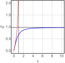
(a)

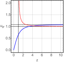
(b)

Figure 7: Group velocity of Eq. (94) of the mode $\oplus$ for the parameters $\beta=1/(2\sqrt{2})$, $\vartheta=\pi/3$ (blue, plain) and for $\beta=1$, $\vartheta=0$ (red, dotted) LABEL:sub@fig:full-theory-complicated-dispersion-equation-spacelike-parallel-case-1. The group velocity of the mode $\ominus$ for the parameter choices $\alpha=1/2$, $\beta=1/(2\sqrt{2})$, $\vartheta=\pi/3$ (plain, blue) and $\alpha=\beta=1$, $\vartheta=0$ (red, dotted) can be found in LABEL:sub@fig:full-theory-complicated-dispersion-equation-spacelike-parallel-case-2. Asymptotes are shown as black, dotted lines.

where these results are expressed in terms of the constant ratios $x/z\equiv\alpha$ and $y/z\equiv\beta$. The front velocity of the mode $\oplus$ cannot exceed 1, which does not hold for the mode $\ominus$, though, as $u_{\mathrm{fr}}^{(-)}$ can be larger than 1 for $\beta<\alpha$. The next step is to obtain the magnitudes of the group velocities:

$$u_{\mathrm{gr}}^{(+)} =\sqrt{\frac{4y^{2}(y^{2}-z^{2})\cos^{2}\vartheta+z^{4}}{z^{2}(1+z^{2}-2y^{2}\cos^{2}\vartheta)}}\,,$$ (94a)

$$u_{\mathrm{gr}}^{(-)} =\sqrt{\frac{4(x^{2}-y^{2})(x^{2}+y^{2}-z^{2})\cos^{2}\vartheta-(2x^{2}-z^{2})^{2}}{(2x^{2}-z^{2})\left[1+z^{2}-2(x^{2}\sin^{2}\vartheta+y^{2}\cos^{2}\vartheta)\right]}}\,,$$ (94b)

with the definitions (87d). By introducing the parameters $\alpha$, $\beta$ into the previous results, the asymptotic behavior of the group velocity for small momenta is

$$u_{\mathrm{gr}}^{(\pm)} =\bar{\bar{\Theta}}^{(\pm)}|\mathbf{p}|\,,$$ (95a)

$$\bar{\bar{\Theta}}^{(+)} =\theta\sqrt{1+4\beta^{2}(\beta^{2}-1)\cos^{2}\vartheta}\,,\quad\bar{\bar{\Theta}}^{(-)}=\theta\sqrt{1-2\alpha^{2}+\frac{4(\alpha^{2}-\beta^{2})[1-(\alpha^{2}+\beta^{2})]\cos^{2}\vartheta}{1-2\alpha^{2}}}\,.$$ (95b)

Each mode again resembles an anisotropic Podolsky mode. The limit of vanishing Lorentz violation leads to the standard Podolsky dispersion relation. Also, the modes can exhibit spurious behavior, since singularities are present for

$$z_{\mathrm{sing}}^{(+)}=\frac{1}{\sqrt{2\beta^{2}\cos^{2}\vartheta-1}}\,,\quad z_{\mathrm{sing}}^{(-)}=\frac{1}{\sqrt{2(\alpha^{2}\sin^{2}\vartheta+\beta^{2}\cos^{2}\vartheta)-1}}\,,$$ (96)

again pointing to the existence of unphysical regimes (see the red curves of Fig. 7). The parameters $\alpha$ and $\beta$ can be chosen such that these values are complex, whereupon there are no singularities. In this case, the group velocity rises from 0 to a finite value. This behavior is characteristic of an exotic mode if this finite value is smaller than 1. The blue curve in Fig. 7a represents an example for this case. If the finite value is larger than 1 the mode is spurious whereby an example is given by the blue curve in Fig. 7b. Each expression for the group velocity exceeds 1 for

$$z|_{u_{\mathrm{gr}}^{(+)}=1}=\frac{1}{\sqrt{4\beta^{2}-2}|\beta\cos\vartheta|}\,,\quad z|_{u_{\mathrm{gr}}^{(-)}=1}=\sqrt{\frac{1-2\alpha^{2}}{(1-2\beta^{2})(\alpha^{2}-\beta^{2})[1+\cos(2\vartheta)]}}\,.$$ (97)

The first value becomes complex for $\beta<1/\sqrt{2}$ and the second for $\alpha>1/\sqrt{2}$, $\beta>1/\sqrt{2}$, and $\beta>\alpha$ at the same time or for $\alpha>1/\sqrt{2}>\beta$ or when $1/\sqrt{2}>\beta>\alpha$. Under these conditions, the group velocity stays below 1. The profiles of $u_{\mathrm{gr}}$ for these two modes are depicted in Fig. 7.

V Connection to nonminimal SME

An interesting question to ask is whether the LV contribution of Lagrangian (3) is contained in the nonminimal SME by Kostelecký and Mewes Kostelec1 . As we are addressing LV and CPT-even dimension-6 terms, the first higher-order LV coefficient to be considered is that of dimension 6, namely

$$(\hat{k}_{F})^{\kappa\lambda\mu\nu}=(k_{F}^{(6)})^{\kappa\lambda\mu\nu\alpha_{1}\alpha_{2}}\partial_{\alpha_{1}}\partial_{\alpha_{2}}\,,$$ (98)

where we have omitted the usual dimension-4 CPT-even coefficients of the photon sector of the SME, $(k_{F}^{(4)})^{\kappa\lambda\mu\nu}$. It is possible to show that the parameterization

$$(k_{F}^{(6)})^{\mu\nu\varrho\sigma\alpha_{1}\alpha_{2}}=\eta^{2}D^{\nu\sigma}g^{\mu\alpha_{1}}g^{\varrho\alpha_{2}}\,,$$ (99a)

successfully reproduces the LV term present in Lagrangian (3). Indeed,

$$(k_{F}^{(6)})^{\mu\nu\varrho\sigma\alpha_{1}\alpha_{2}}\partial_{\alpha_{1}}\partial_{\alpha_{2}}F_{\mu\nu}F_{\rho\sigma}=\eta^{2}D^{\nu\sigma}\partial^{\mu}\,F_{\mu\nu}\partial^{\varrho}F_{\rho\sigma}\,,$$ (99b)

which demonstrates that this LV piece is contained in the nonminimal SME Kostelec1 . In an analogue way, the correspondence

$$(k_{F}^{(6)})^{\mu\nu\varrho\sigma\alpha_{1}\alpha_{2}}=\eta_{1}^{2}D^{\nu\sigma}g^{\mu\alpha_{1}}g^{\varrho\alpha_{2}}-\eta_{2}^{2}D^{\alpha_{2}\sigma}g^{\mu\alpha_{1}}g^{\nu\varrho}\,,$$ (100)

yields the LV terms of the generalized model of Lagrangian (68). Finally, the symmetries of $(\hat{k}_{F})^{\kappa\lambda\mu\nu}$ have to be taken into account. The latter fourth-rank observer tensor is antisymmetric in the first and second pair of indices and symmetric under an exchange of both index pairs, which is evidently not the case for the choices in Eqs. (99), (100). Performing the (anti)symmetrization explicitly and considering the factor 1/4 before $(\hat{k}_{F})^{\kappa\lambda\mu\nu}$ in the definition of the $CPT$-even term of the SME photon sector, the final mapping of our terms to the SME is given by

$$(\hat{k}_{F})^{\mu\nu\varrho\sigma} = \frac{1}{2}\left[(k_{F}^{(6)})^{\mu\nu\varrho\sigma\alpha_{1}\alpha_{2}}-(k_{F}^{(6)})^{\nu\mu\varrho\sigma\alpha_{1}\alpha_{2}}-(k_{F}^{(6)})^{\mu\nu\sigma\varrho\alpha_{1}\alpha_{2}}+(k_{F}^{(6)})^{\nu\mu\sigma\varrho\alpha_{1}\alpha_{2}}\right.$$ (101)

$$\left.\phantom{\frac{1}{2}\Big{[}}+\,(\mu\leftrightarrow\varrho,\nu\leftrightarrow\sigma)\right]\partial_{\alpha_{1}}\partial_{\alpha_{2}}\,.$$

It can be checked that the tensor constructed in this way automatically satisfies the Bianchi identity for an arbitrary triple of indices chosen from the first four indices. In addition, antisymmetrization on any three indices must be imposed via Eq. (55) of the first paper in Kostelec1 . The Podolsky term is Lorentz-invariant and cannot be mapped to SME coefficients. However, it is introduced into the field equations of the nonminimal $CPT$-even photon sector as follows:

$$M^{\mu\nu}A_{\nu} =0\,,$$ (102a)

$$M^{\mu\nu} =\left\{(1-\theta^{2}p^{2})\left[g^{\mu\nu}g^{\alpha\beta}-g^{\mu\alpha}g^{\nu\beta}\right]+2(\hat{k}_{F})^{\mu\alpha\nu\beta}\right\}p_{\alpha}p_{\beta}\,.$$ (102b)

VI Conclusion and remarks

In this work we have addressed an electrodynamics endowed with LV terms of mass dimension 6. We considered aspects not yet analysed in the literature, such as an evaluation of the propagator, the dispersion relations, and the propagation modes. First, a Maxwell electrodynamics modified by an anisotropic Podolsky-type term of mass dimension 6 was examined. For certain parameter choices, all the modes, which are affected by the higher-dimensional term, were found to exhibit a nonphysical behavior. The magnitude of the group velocity was demonstrated to become larger than 1 (breaking of causality), to have singularities or to vanish for small momenta (absence of propagation). The first two behaviors described are interpreted as unphysical and we referred to dispersion relations having characteristics of this kind as spurious. Features such as decreasing group or front velocities for small momenta only indicate that these modes decouple from the low-energy regime. According to the criteria used in the paper, a mode endowed with such properties was called exotic as long as it neither involved singularities nor superluminal group or front velocities.

The results obtained indicate that an electrodynamics modified by this kind of higher-derivative LV term can only provide a physical propagation of signals in the limit of large momenta. Such an interpretation could recover a meaningful behavior of the theory in the case that it is possible to state a suitable cutoff without generating bad side effects. For small momenta, some of the modes correspond to Lorentz-violating modifications of the Podolsky-type dispersion relation, which are not necessarily unphysical. We also found dispersion relations providing group velocities that are larger than 1 or divergent at some points, which are behaviors characterizing spurious propagation modes. A brief discussion of unitarity for this modification was delivered as well. The result of our analysis was that additional time derivatives in the Lagrange density are likely to spoil unitarity. This behavior is expected and was already observed in Lorentz-invariant higher-derivative theories as well as alternative LV higher-derivative modifications of the photon and fermion sector.

At a second stage, we analyzed a more general extension of the modified electrodynamics in the presence of an additional anisotropic Lee-Wick term of mass dimension 6. Again, the propagator was derived and the corresponding dispersion relations were obtained from it. Subsequently, these dispersion relations were examined with respect to signal propagation. The structure of this second framework is more involved in comparison to the first theory under consideration. The modified dispersion relations are associated with exotic and spurious modes, as already observed in the first model. There exist parameter choices that are connected to issues with causality. Another observation was that some of the dispersion relations can exhibit singularities, i.e., they become unphysical for a certain range of momenta, which is enough to classify these modes as spurious. However, we also found sectors for which the dispersion laws do not suffer from any of the problems just mentioned. Therefore, those can be considered as well-behaved according to the criteria that the current paper is based on.

The results of the paper suggest which sectors of the framework should be subject to quantization and which ones should be discarded. These sectors are classified according to the geometrical properties of the two four-vectors that the background tensor is composed of. Both spurious and exotic modes were found dependent on choices of the parameters. There is no need of introducing lower cutoffs of the four-momentum, which would be difficult to realize from a physical point of view, anyhow. Instead, the regions of parameter space associated with a vicious classical behavior should be removed from the theory. If the theories proposed are subject to studies at the quantum level in the future, the results of the paper demonstrate, which sectors could be quantized properly. Physical dispersion relations must be clearly free of singularities. Modes without violations of classical causality may be the preferred ones to be studied. However, it ought to be taken into account, as well, that superluminal velocities do not necessarily cause problems at the quantum level, e.g., for microcausality Klinkhamer:2010zs .

One of the most significant questions to be answered in future works would be related to gauge fixing. It was mentioned in the paper that gauge fixing in vector field theories including higher derivatives is even more subtle than in the standard case. Whether or not the gauge fixing conditions proposed in GalvaoP for Podolsky’s theory are still applicable in the Lorentz-violating case, would be an interesting aspect to investigate. Furthermore, to quantize the theory, proper field operators will have to be constructed and a treatment of the spurious dispersion laws at the quantum level would be mandatory. A related question is whether the prescription of how to preserve (perturbative) unitarity, which was introduced by Lee and Wick LeeWick , still works. Finally, the free theory should be coupled to fermions to be able to study physical processes. Such questions have been considered recently for a particular fermionic framework including higher derivatives Reyes:2016pus , but how to proceed in the photon sector is still an open problem.

- (1) D. Colladay and V.A. Kostelecký, Phys. Rev. D 55, 6760 (1997); D. Colladay and V.A. Kostelecký, Phys. Rev. D 58, 116002 (1998); S.R. Coleman and S.L. Glashow, Phys. Rev. D 59, 116008 (1999).
- (2) V.A. Kostelecký and S. Samuel, Phys. Rev. Lett. 63, 224 (1989); Phys. Rev. D 39, 683 (1989); Phys. Rev. D 40, 1886 (1989); Phys. Rev. Lett. 66, 1811 (1991); V.A. Kostelecký and R. Potting, Nucl. Phys. B 359, 545 (1991); Phys. Rev. D 51, 3923 (1995); Phys. Lett. B 381, 89 (1996).
- (3) V.A. Kostelecký and C.D. Lane, J. Math. Phys. 40, 6245 (1999); V.A. Kostelecký and R. Lehnert, Phys. Rev. D 63, 065008 (2001); D. Colladay and V.A. Kostelecký, Phys. Lett. B 511, 209 (2001); R. Lehnert, Phys. Rev. D 68, 085003 (2003); R. Lehnert, J. Math. Phys. 45, 3399 (2004); B. Altschul, Phys. Rev. D 70, 056005 (2004); G.M. Shore, Nucl. Phys. B 717, 86 (2005).
- (4) W.F. Chen and G. Kunstatter, Phys. Rev. D 62, 105029 (2000); O.G. Kharlanov and V.Ch. Zhukovsky, J. Math. Phys. 48, 092302 (2007); B. Gonçalves, Y.N. Obukhov, and I.L. Shapiro, Phys. Rev. D 80, 125034 (2009); S.I. Kruglov, Phys. Lett. B 718, 228 (2012); T.J. Yoder and G.S. Adkins, Phys. Rev. D 86, 116005 (2012); S. Aghababaei, M. Haghighat, I. Motie, Phys. Rev. D 96, 115028 (2017).
- (5) R. Bluhm, V.A. Kostelecký, and N. Russell, Phys. Rev. Lett. 79, 1432 (1997); R. Bluhm, V.A. Kostelecký, and N. Russell, Phys. Rev. D 57, 3932 (1998); R. Bluhm, V.A. Kostelecký, and N. Russell, Phys. Rev. Lett. 82, 2254 (1999); V.A. Kostelecký and C.D. Lane, Phys. Rev. D 60, 116010 (1999); R. Bluhm and V.A. Kostelecký, Phys. Rev. Lett. 84, 1381 (2000); R. Bluhm, V.A. Kostelecký, and C.D. Lane, Phys. Rev. Lett. 84, 1098 (2000); R. Bluhm, V.A. Kostelecký, C.D. Lane, and N. Russell, Phys. Rev. Lett. 88, 090801 (2002).
- (6) S.M. Carroll, G.B. Field, and R. Jackiw, Phys. Rev. D 41, 1231 (1990); A.A. Andrianov and R. Soldati, Phys. Rev. D 51, 5961 (1995); A.A. Andrianov and R. Soldati, Phys. Lett. B 435, 449 (1998); A.A. Andrianov, R. Soldati, and L. Sorbo, Phys. Rev. D 59, 025002 (1998); C. Adam and F.R. Klinkhamer, Nucl. Phys. B 607, 247 (2001); C. Adam and F.R. Klinkhamer, Nucl. Phys. B 657, 214 (2003); V.Ch. Zhukovsky, A.E. Lobanov, and E.M. Murchikova, Phys. Rev. D 73, 065016 (2006); A.A. Andrianov, D. Espriu, P. Giacconi, and R. Soldati, J. High Energy Phys. 0909, 057 (2009); J. Alfaro, A.A. Andrianov, M. Cambiaso, P. Giacconi, and R. Soldati, Int. J. Mod. Phys. A 25, 3271 (2010); Y.M.P. Gomes, P.C. Malta, Phys. Rev. D 94, 025031 (2016); A. Martín-Ruiz, C.A. Escobar, Phys. Rev. D 95, 036011 (2017).
- (7) A.P. Baêta Scarpelli, H. Belich, J.L. Boldo, and J.A. Helayël-Neto, Phys. Rev. D 67, 085021 (2003); R. Lehnert and R. Potting, Phys. Rev. Lett. 93, 110402 (2004); R. Lehnert and R. Potting, Phys. Rev. D 70, 125010 (2004); C. Kaufhold and F.R. Klinkhamer, Nucl. Phys. B 734, 1 (2006); B. Altschul, Phys. Rev. D 75, 105003 (2007); H. Belich, L.D. Bernald, P. Gaete, and J.A. Helayël-Neto, Eur. Phys. J. C 73, 2632 (2013).
- (8) B. Altschul, Phys. Rev. Lett. 98, 041603 (2007); C. Kaufhold and F.R. Klinkhamer, Phys. Rev. D 76, 025024 (2007); B. Altschul, Nucl. Phys. B 796, 262 (2008).
- (9) V.A. Kostelecký and M. Mewes, Phys. Rev. Lett. 87, 251304 (2001); V.A. Kostelecký and M. Mewes, Phys. Rev. D 66, 056005 (2002); V.A. Kostelecký and M. Mewes, Phys. Rev. Lett. 97, 140401 (2006); C.A. Escobar and M.A.G. Garcia, Phys. Rev. D 92, 025034 (2015); A. Martín-Ruiz and C.A. Escobar, Phys. Rev. D 94, 076010 (2016).
- (10) B. Altschul, Phys. Rev. Lett. 98, 041603 (2007); C. Kaufhold and F.R. Klinkhamer, Phys. Rev. D 76, 025024 (2007); F.R. Klinkhamer and M. Risse, Phys. Rev. D 77, 016002 (2008); F.R. Klinkhamer and M. Risse, Phys. Rev. D 77, 117901 (2008); F.R. Klinkhamer and M. Schreck, Phys. Rev. D 78, 085026 (2008).
- (11) A. Moyotl, H. Novales-Sánchez, J.J. Toscano, and E.S. Tututi, Int. J. Mod. Phys. A 29, 1450039 (2014); Int. J. Mod. Phys. A 29, 1450107 (2014).
- (12) M. Schreck, Phys. Rev. D 86, 065038 (2012); G. Gazzola, H.G. Fargnoli, A.P. Baêta Scarpelli, M. Sampaio, and M.C. Nemes, J. Phys. G 39, 035002 (2012); A.P. Baêta Scarpelli, J. Phys. G 39, 125001 (2012); B. Agostini, F.A. Barone, F.E. Barone, P. Gaete, and J.A. Helayël-Neto, Phys. Lett. B 708, 212 (2012); L.C.T. Brito, H.G. Fargnoli, and A.P. Baêta Scarpelli, Phys. Rev. D 87, 125023 (2013).
- (13) R. Jackiw and V.A. Kostelecký, Phys. Rev. Lett. 82, 3572 (1999); J.-M. Chung, Phys. Rev. D 60, 127901 (1999); M. Pérez-Victoria, Phys. Rev. Lett. 83, 2518 (1999); J.-M. Chung and B.K. Chung, Phys. Rev. D 63, 105015 (2001); G. Bonneau, Nucl. Phys. B 593, 398 (2001); M. Pérez-Victoria, J. High Energy Phys. 0104, 032 (2001); O.A. Battistel and G. Dallabona, J. Phys. G 27, L53 (2001); Nucl. Phys. B 610, 316 (2001); A.P.B. Scarpelli, M. Sampaio, M.C. Nemes, and B. Hiller, Phys. Rev. D 64, 046013 (2001); O.A. Battistel and G. Dallabona, J. Phys. G 28, L23 (2002); B. Altschul, Phys. Rev. D 70, 101701(R) (2004); T. Mariz, J.R. Nascimento, E. Passos, R.F. Ribeiro, and F.A. Brito, J. High Energy Phys. 0510, 019 (2005); J.R. Nascimento, E. Passos, A.Yu. Petrov, and F.A. Brito, J. High Energy Phys. 0706, 016 (2007); A.P.B. Scarpelli, M. Sampaio, M.C. Nemes, and B. Hiller, Eur. Phys. J. C 56, 571 (2008); F.A. Brito, J.R. Nascimento, E. Passos, and A.Yu. Petrov, Phys. Lett. B 664, 112 (2008); F.A. Brito, L.S. Grigorio, M.S. Guimaraes, E. Passos, and C. Wotzasek, Phys. Rev. D 78, 125023 (2008); O.M. Del Cima, J.M. Fonseca, D.H.T. Franco, and O. Piguet, Phys. Lett. B 688, 258 (2010).
- (14) V.A. Kostelecký and M. Mewes, Phys. Rev. D 80, 015020 (2009); M. Mewes, Phys. Rev. D 85, 116012 (2012); M. Schreck, Phys. Rev. D 89, 105019 (2014).
- (15) V.A. Kostelecký and M. Mewes, Phys. Rev. D 88, 096006 (2013); M. Schreck, Phys. Rev. D 90, 085025 (2014).
- (16) R.C. Myers and M. Pospelov, Phys. Rev. Lett. 90, 211601 (2003); C.M. Reyes, L.F. Urrutia, and J.D. Vergara, Phys. Rev. D 78, 125011 (2008); J. Lopez-Sarrion and C.M. Reyes, Eur. Phys. J. C 72, 2150 (2012).
- (17) C.M. Reyes, L.F. Urrutia, and J.D. Vergara, Phys. Lett. B 675, 336 (2009); C.M. Reyes, Phys. Rev. D 82, 125036 (2010); C.M. Reyes, Phys. Rev. D 87, 125028 (2013).
- (18) H. Belich, T. Costa-Soares, M.M. Ferreira, Jr., and J.A. Helayël-Neto, Eur. Phys. J. C 41, 421 (2005); H. Belich, L.P. Colatto, T. Costa-Soares, J.A. Helayël-Neto, and M.T.D. Orlando, Eur. Phys. J. C 62, 425 (2009); B. Charneski, M. Gomes, R.V. Maluf, and A.J. da Silva, Phys. Rev. D 86, 045003 (2012); A.F. Santos, and Faqir C. Khanna, Phys. Rev. D 95, 125012 (2017).
- (19) R. Casana, M.M. Ferreira, Jr., E. Passos, F.E.P. dos Santos, and E.O. Silva, Phys. Rev. D 87, 047701 (2013); J.B. Araujo, R. Casana, M.M. Ferreira, Jr., Phys. Lett. B 760, 302 (2016).
- (20) Y. Ding and V.A. Kostelecký, Phys. Rev. D 94, 056008 (2016).
- (21) B. Podolsky, Phys. Rev. 62, 68 (1942); B. Podolsky and C. Kikuchi, Phys. Rev. 65, 228 (1944).
- (22) A. Accioly and E. Scatena, Mod. Phys. Lett. A 25, 269 (2010).
- (23) C.A.P. Galvão and B.M. Pimentel, Can. J. Phys. 66, 460 (1988).
- (24) R. Bufalo, B.M. Pimentel, and G.E.R. Zambrano, Phys. Rev. D 83, 045007 (2011).
- (25) C.A. Bonin, R. Bufalo, B.M. Pimentel, and G.E.R. Zambrano, Phys. Rev. D 81, 025003 (2010).
- (26) R. Bufalo, B.M. Pimentel, and G.E.R. Zambrano, Phys. Rev. D 86, 125023 (2012).
- (27) C.A. Bonin, B.M. Pimentel, and P.H. Ortega, “Multipole expansion in generalized electrodynamics,” arXiv:1608.00902.
- (28) T.D. Lee and G.C. Wick, Nucl. Phys. B 9, 209 (1969); T.D. Lee and G.C. Wick, Phys. Rev D 2, 1033 (1970).
- (29) B. Grinstein and D. O’Connell, Phys. Rev. D 78, 105005 (2008); B. Grinstein, D. O’Connell, and M.B. Wise, Phys. Rev. D 77, 025012 (2008); J.R. Espinosa, B. Grinstein, D. O’Connell, and M.B. Wise, Phys. Rev. D 77, 085002 (2008); T.E.J. Underwood and R. Zwicky, Phys. Rev. D 79, 035016 (2009); R.S. Chivukula, A. Farzinnia, R. Foadi, and E.H. Simmons, Phys. Rev. D 82, 035015 (2010).
- (30) T.G. Rizzo, J. High Energy Phys. 0706, 070 (2007); T.G. Rizzo, J. High Energy Phys. 0801, 042 (2008); E. Álvarez, C. Schat, L. Da Rold, and A. Szynkman, J. High Energy Phys. 0804, 026 (2008); C.D. Carone and R. Primulando, Phys. Rev. D 80, 055020 (2009).
- (31) A.M. Shalaby, Phys. Rev. D 80, 025006 (2009).
- (32) C.D. Carone, Phys. Lett. B 677, 306 (2009); C.D. Carone and R.F. Lebed, J. High Energy Phys. 0901, 043 (2009).
- (33) B. Grinstein and D. O’Connell, Phys. Rev. D 78, 105005 (2008); R.S. Chivukula, A. Farzinnia, R. Foadi, and E.H. Simmons, Phys. Rev. D 82, 035015 (2010).
- (34) B. Fornal, B. Grinstein, and M.B. Wise, Phys. Lett. B 674, 330 (2009); C.A. Bonin, R. Bufalo, B.M. Pimentel, and G.E.R. Zambrano, Phys. Rev. D 81, 025003 (2010); C.A. Bonin and B.M. Pimentel, Phys. Rev. D 84, 065023 (2011).
- (35) A.A. Slavnov, Teor. Mat. Fiz 13, 174 (1972).
- (36) F.A. Barone, G. Flores-Hidalgo, and A.A. Nogueira, Phys. Rev. D 88, 105031 (2013).
- (37) F.A. Barone, G. Flores-Hidalgo, and A.A. Nogueira, Phys. Rev. D 91, 027701 (2015).
- (38) F.A. Barone and A.A. Nogueira, Eur. Phys. J. C 75, 339 (2015).
- (39) A. Accioly, J. Helayël-Neto, F.E. Barone, F.A. Barone, and P. Gaete, Phys. Rev. D 90, 105029 (2014).
- (40) L.H.C. Borges, A.G. Dias, A.F. Ferrari, J.R. Nascimento, and A.Yu. Petrov, Phys. Lett. B 756, 332 (2016).
- (41) L.H.C. Borges, A.F. Ferrari, and F.A. Barone, Eur. Phys. J. C 76, 599 (2016).
- (42) V.A. Kostelecký and N. Russell, Rev. Mod. Phys. 83, 11 (2011).
- (43) L. Bonetti, L.R. dos Santos Filho, J.A. Helayël-Neto, and A.D.A.M. Spallicci, Phys. Lett. B 764, 203 (2017).
- (44) A.P. Baêta Scarpelli, H. Belich, J.L. Boldo, and J.A. Helayël-Neto, Phys. Rev. D 67, 085021 (2003); R. Casana, M.M. Ferreira, Jr., A.R. Gomes, and F.E.P. dos Santos, Phys. Rev. D 82, 125006 (2010); R. Casana, M.M. Ferreira, Jr., and R.P.M. Moreira, Eur. Phys. J. C 72, 2070 (2012); A. Moyotl, H. Novales-Sánchez, J.J. Toscano, and E.S. Tututi, Int. J. Mod. Phys. A 29, 1450107 (2014); T.R.S. Santos, R.F. Sobreiro, and A.A. Tomaz, Phys. Rev. D 94, 085027 (2016).
- (45) J.A.M. Vermaseren, “New features of FORM,” math-ph/0010025.
- (46) L. Brillouin, Wave propagation and group velocity (Academic Press, New York and London, 1960).
- (47) F.R. Klinkhamer and M. Schreck, Nucl. Phys. B 848, 90 (2011).
- (48) C.M. Reyes and L.F. Urrutia, Phys. Rev. D 95, 015024 (2017); M. Maniatis and C.M. Reyes, Phys. Rev. D 89, 056009 (2014); C.M. Reyes, Phys. Rev. D 87, 125028 (2013).
- (49) R. Turcati and M.J. Neves, Adv. High Energy Phys. 153953, 1 (2014).
- (50) M. Veltman, in Methods in Field Theory, edited by R. Balian and J. Zinn-Justin (World Scientific, Singapore, 1981).
- (51) D. Colladay and V.A. Kostelecký, Phys. Lett. B 511, 209 (2001).