Single-pulse observations of the Galactic Center magnetar PSR J1745$-$2900 at 3.1 GHz

Abstract

We report on single-pulse observations of the Galactic Center magnetar PSR J1745$-$2900 that were made using the Parkes 64-m radio telescope with a central frequency of 3.1 GHz at five observing epochs between 2013 July and August. The shape of the integrated pulse profiles was relatively stable across the five observations, indicating that the pulsar was in a stable state between MJDs 56475 and 56514. This extends the known stable state of this pulsar to 6.8 months. Short term pulse shape variations were also detected. It is shown that this pulsar switches between two emission modes frequently and that the typical duration of each mode is about ten minutes. No giant pulses or subpulse drifting were observed. Apparent nulls in the pulse emission were detected on MJD 56500. Although there are many differences between the radio emission of magnetars and normal radio pulsars, they also share some properties. The detection of mode changing and pulse nulling in PSR J1745$-$2900 suggests that the basic radio emission process for magnetars and normal pulsars is the same.

1 Introduction

Magnetars are commonly considered to be rotating neutron stars whose inferred surface dipolar magnetic fields are extremely strong (typically $10^{14}$ – $10^{15}$ G) (Duncan & Thompson, 1992). Their X-ray and $\gamma$-ray luminosities are usually orders of magnitude larger than their spin-down luminosity. It is believed that magnetar emission, particularly at high energies, is powered by the decay of the enormous magnetic fields (Thompson & Duncan, 1995, 1996) instead of by the spin-down. However, the discoveries of low magnetic field magnetars (Rea et al., 2010, 2012, 2014) may challenge the original assumption that a high surface dipolar magnetic field strength is required for the activity of a typical magnetar.

The magnetar group is classified by observers as Soft Gamma Repeaters (SGRs) and Anomalous X-ray Pulsars (AXPs), and both subgroups are typically detected at high energies. The total number of magnetars currently known is 29 (Olausen & Kaspi, 2014). To date, only four of them have shown pulsed radio emmision (Camilo et al., 2006, 2007b; Levin et al., 2010; Shannon & Johnston, 2013; Eatough et al., 2013). PSR J1745$-$2900 is the newest radio-emitting magnetar. It was serendipitously discovered by the Swift telescope as an X-ray flare that came from the region near Sagittarius A* (Sgr A*) (Kennea et al., 2013). Subsequent observations of PSR J1745$-$2900 by the NuSTAR telescope revealed pulsed X-ray emission with a spin period of 3.76 s and a spin-down rate of $\dot{P}=6.5\times 10^{-12}$, which implies a surface dipolar magnetic field $B=1.6\times 10^{14}\ \mathrm{G}$. This confirmed PSR J1745$-$2900 as a magnetar in the Galactic center (GC) region (Mori et al., 2013). With a series of observations with the Chandra and the Swift telescopes, this pulsar was later localized only $2\aas@@fstack{\prime\prime}4$ away from Sgr A* (Rea et al., 2013).

Radio pulsations from PSR J1745$-$2900 were subsequently detected with many radio tesescopes. Shannon & Johnston (2013) and Eatough et al. (2013) reported multifrequency radio observations of PSR J1745$-$2900 and showed that it has the largest dispersion measure (DM = $1778\ \pm 3\ \mathrm{cm^{-3}\ pc}$) and rotation measure (RM = $-66960\ \pm\ 50\ \mathrm{rad\ m^{-2}}$) of any known pulsar. These measurements constrain the strength of the magnetic field near the GC. Based on high-resolution astrometry measurements for PSR J1745$-$2900 with the VLBA and VLA, Bower et al. (2014) found that the angular broadening for this pulsar is in good agreement with that of Sgr A*, confirming that PSR J1745$-$2900 and Sgr A* must be close to each other to share a similar scattering medium. The proper motion of PSR J1745$-$2900 relative to Sgr A* was later measured by the VLBA observations. Bower et al. (2015) demonstrated that this pulsar has a transverse velocity of 236 km s^-1 at a projected separation of 0.097 pc from Sgr A*. Radio observations indicated that PSR J1745$-$2900 has a relatively flat radio spectrum making the pulsar detectable at millimeter bands (Torne et al., 2015, 2017). Single-pulse radio observations for PSR J1745$-$2900 were carried out by Lynch et al. (2015) and Yan et al. (2015) at frequencies above 8 GHz using the GBT and the Shanghai Tian Ma Radio Telescope (TMRT) respectively. Their results showed that the radio radiative activity of the pulsar underwent a change from a fairly stable state to a more erratic state. Both the flux density and the pulse profile morphology showed substantial changes from epoch to epoch in the erratic phase. No giant pulses or subpulse drifting were detected in these observations.

The NE2001 model predicts a very large scattering timescale for PSR J1745$-$2900. PSR J1745$-$2900 would be undetectable at frequencies below 5 GHz if the prediction of the NE2001 model were true. But the observed scattering broadening was much lower than this prediction (Spitler et al., 2014; Pennucci et al., 2015), implying that radio pulsations may be detectable at relatively low frequencies. The new YWM16 model (Yao et al., 2017) predicts the scattering observed in J1745$-$2900 very well, based on the scattering results of Krishnakumar et al. (2015). In this paper, we present the results of single-pulse observations at 3.1 GHz for PSR J1745$-$2900 that were made with the Parkes 64-m radio telescope, which is the lowest frequency single-pulse analysis for this pulsar to date. Details of the observing system and the observations are given in Section 2. The mean pulse profile and single-pulse properties are shown in Section 3. The implications of the results are discussed in Section 4.

2 Observations

Table 1: Summary of the observations. Note that the symbols $\tau_{\mathrm{samp}}$ and T_obs represent the sampling interval and the duration of the observation respectively. For details about Project ID, see descriptions in the Parkes Pulsar Data Archive.

Date	MJD	Project	Frequency	Bandwidth	No. of	$\tau_{\mathrm{samp}}$	Tobs
(yyyy-mm-dd)	(d)	ID	(MHz)	(MHz)	Channels	($\mu$s)	(min)
2013-07-02	56475	P626	3100	1024	512	256	101
2013-07-19	56492	P574	3094	1024	512	256	20
2013-07-21	56494	P574	3094	1024	512	256	20
2013-07-27	56500	P626	3100	1024	512	128	160
2013-08-10	56514	P456	3094	1024	512	128	13

As the only known pulsar that is located at the GC, PSR J1745$-$1900 has been observed many times at multiple frequency bands by the Parkes 64-m radio telescope for many projects. Many of those data are publicly available in the Parkes Pulsar Data Archive (Hobbs et al., 2011). High signal-to-noise ratio (S/N) and long duration are the essential criteria for the selection of observational data to study single pulses. Under these criteria, five single-pulse observations of PSR J1745$-$2900 made between 2013 July and August were found in the Parkes Pulsar Data Archive and then analyzed in this paper. Unfortunately, no suitable calibration observation can be found in the Parkes Pulsar Data Archive for the five observations, so flux and polarization calibration cannot be performed here. The five observations were taken with the 10-cm receiver, which has a bandwidth of 1024 MHz centred around 3.1 GHz, and the fourth generation Parkes digital filterbank system PDFB4. Details of the observations are summarized in Table 1. The full bandwidth was divided into 512 channels to allow incoherent de-dispersion, resulting in a 2-MHz channel width and hence a 0.98-ms dispersive time delay across each frequency channel at 3.1 GHz for PSR J1745$-$2900 (Lorimer & Kramer, 2005). This dispersion smear time is two orders of magnitude less than the observed average half-power width of single pulses, so 512 channels are sufficient for us.

The data were reduced using the DSPSR package (van Straten & Bailes, 2011) to de-disperse and produce single-pulse integrations which preserve information on individual pulses. The pulsar’s rotational ephemeris was taken from (Lynch et al., 2015) and the single-pulse integrations were recorded using the PSRFITS data format (Hotan et al., 2004) with 1024 phase bins per rotation period. Radio frequency interference (RFI) in the single-pulse archives was removed in affected frequency channels and time sub-integrations using PAZ and PAZI programs of the pulsar analysis system PSRCHIVE (Hotan et al., 2004). Even after this, the observed profile baselines varied significantly probably because of residual low-level RFI. We removed the effect of the varying baseline by subtracting the mean level in the off-pulse window adjacent to the pulse from each single-pulse integration. The single-pulse analysis was carried out with the PSRSALSA package (Weltevrede, 2016) which is freely available online. The single-pulse integrations were rebinned from 1024 to 512 pulse phase bins to increase the S/N.

3 Results

We present and discuss the mean pulse profile and single-pulse properties for PSR J1745$-$1900 in this section. As mentioned in Section 2, we cannot perform analyses of polarization properties and absolute flux densities for this pulsar since no calibration data are available.

3.1 Mean pulse profiles

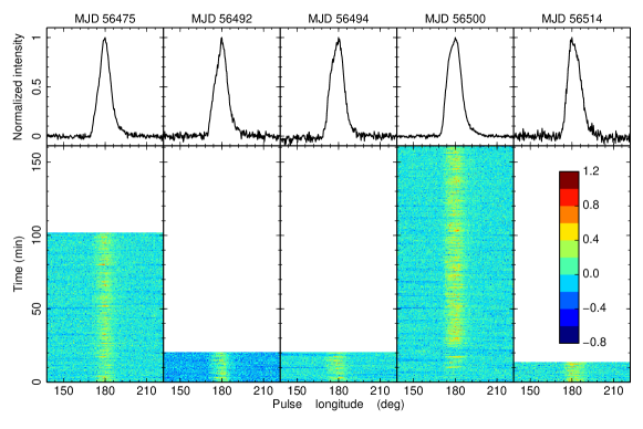
Figure 1: 3.1-GHz single-pulse stacks (lower) and corresponding mean pulse profiles (upper) of PSR J1745$-$2900 observed at five observing epochs. The flux density of each mean pulse profile is normalized by its peak flux density. The MJD for the day of observation is presented at the top of each subplot.

Even though the DM of PSR J1745$-$1900 is as large as $1778\ \mathrm{cm^{-3}\ pc}$, the integrated pulse profile of PSR J1745$-$1900 above 2 GHz is dominated by pulse jitter rather than scattering (Spitler et al., 2014). Based on eight months GBT observations, Lynch et al. (2015) identified two periods of radio radiative activity for PSR J1745$-$1900 : a stable state (covering MJDs 56515 - 56682) and an erratic state (covering MJDs 56726 - 56845). In the stable state, the evolution of the spin, radio flux density and profile shape remained relatively stable, while in the erratic state, these properties varied dramatically.

The mean pulse profiles and single-pulse stacks of PSR J1745$-$1900 derived from the five Parkes observations are given in Figure 1. Apart from small variations discussed below, the pulse profile remained steady over the span of the observations, suggesting that the pulsar was in the stable phase. The observations presented here all occurred prior to the stable state defined by Lynch et al. (2015) (see Table 1). This means that our results extend the beginning of the stable state from MJD 56515 to MJD 56475, so the stable state lasted for at least 6.8 months instead of the 5.5 months reported by Lynch et al. (2015).

The mean pulse profiles presented in Figure 1 are single peaked, consistent with early radio observations. Pulse profiles of PSR J1745$-$1900 obtained by early radio observations had a single peak over a wide range of frequency (Shannon & Johnston, 2013; Spitler et al., 2014). Later pulse profiles observed at the GBT at 8.7 GHz showed two peaks in the stable state (Lynch et al., 2015). This led Lynch et al. (2015) to suggest that the pulse profile may have evolved from single to double peaked.

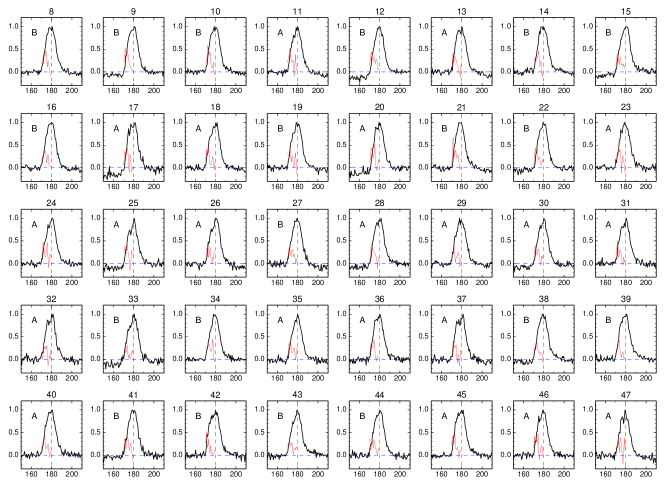
Figure 2: A sequence of 40 sub-integration profiles of PSR J1745$-$2900 with the sub-integration number on top, each averaged over 199.5 seconds. The red line represents the slope of the leading edge for each sub-integration profile. The profile and slope zero are shown by the horizontal dashed line and the vertical dashed line represents the longitude of the peak of the integrated profile.

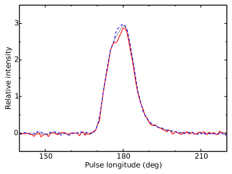
Figure 3: Mean pulse profiles of J1745$-$2900 for mode A (solid), mode B (dashed) and the two modes superimposed (dotted).

Although the mean pulse profile remains stable on a long time-scale (on the order of several months) during the stable state, short time-scale non-random pulse shape variations are visible in the single pulse plots of Figure 1. To investigate the short term pulse shape variations, high S/N sub-integration profiles are needed. When the sub-integration time is less than 130 s, most sub-integration profiles are dominated by pulse jitter and therefore no systematic pulse shape variations can be seen. By visual inspection, we find that sub-integration profiles with sub-integration times between 150 s to 250 s show similar systematic pulse shape variations and so we chose a sub-integration time of 200 s (53 individual pulses) to study the short time-scale changes in pulse shape. A selection of these sub-integration profiles is shown in Figure 2. Some profiles (e.g. Nos. 24, 25 and 26) show a strong main peak and a relatively weak but significant secondary peak on the leading edge of the pulse profile, and we classified these sub-integrations as mode A. Some sub-integration profiles (e.g. Nos. 14, 15 and 16) show a single peak and we classified these sub-integrations as mode B. To distinguish mode A and mode B more rigorously, we used a method based on the point-to-point slope of the leading edge to determine whether a profile has a significant secondary peak on the leading edge or not. The slope at a given point is calculated by taking the average of the slopes between that point and its two closest neighbors. If there is a significant secondary peak on the leading edge, indicating mode A, the slope will be negative at at least one point around the trailing edge of the secondary peak. If the slope does not go negative, the profile is designated as mode B. Using this method, we divided sub-integration profiles shown in Figure 2 into the two modes.

The duration of each mode is typically about ten minutes. However, we cannot obtain the exact duration of each mode because of S/N limitations. Emission modes shorter than 200 s may exist and may be mixed with the other mode within a 200 s sub-integration. Sub-integration profiles Nos. 19, 33, 43 and 44 in Figure 2 may have mixed modes. There are hints of a secondary peak on the leading edge of these four profiles, but their secondary peaks are too weak to be reflected by the slope curve.

Mean pulse profiles for the two modes are given in Figure 3. The mean pulse profile of mode A is double peaked with a relatively weak leading peak while the mean pulse profile of mode B is single peaked.

3.2 Single pulses

Single-pulse properties of PSR J1745$-$1900 are presented in this subsection.

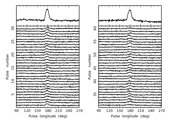
Figure 4: Two contiguous sequences of successive individual pulses of PSR J1745$-$2900 with their corresponding integrated profiles at the top.

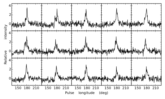
Figure 5: Total intensity profiles for the fifteen highest peak S/N individual pulses of PSR J1745$-$2900 observed on MJD 56500.

Figure 4 shows two contiguous sequences of successive individual pulses of PSR J1745$-$2900 and their corresponding integrated profiles from the observation of MJD 56500. Each sequence contains 30 consecutive single pulses. Single-pulse profiles of the fifteen highest peak S/N pulses of PSR J1745$-$2900 observed on MJD 56500 are presented in Figure 5. Similarly to Esamdin et al. (2012), the peak S/N is calculated as the ratio between the pulse peak amplitude in a given rotation period and the standard deviation of the baseline points in the same period.

3.2.1 Single-pulse energy distribution

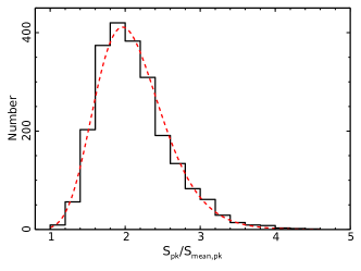
Figure 6: Distribution of the peak flux density of pulses that have peak S/N $\geq$ 4 for the five observations, normalized by the peak flux density of the mean pulse profile at that epoch. The dashed line represents the best-fitting log-normal curve.

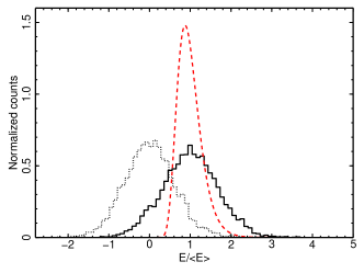
Figure 7: Normalized pulse energy distributions for the five observations. The solid, dotted and dashed lines represent the observed on-pulse energy distribution, the noise energy distribution, and the modelled intrinsic pulse energy distribution with a log-normal function, respectively.

We present a statistical analysis of the energy distribution of single pulses of the five observations. The peak flux density distribution of pulses with peak S/N $\geq$ 4 is presented in Figure 6, and the normalized pulse energy distribution of all pulses is presented in Figure 7.

Following Lynch et al. (2015) and Yan et al. (2015), we normalized the peak flux density of each individual pulse, $\mathrm{S_{pk}}$, with the peak flux density of the mean pulse profile at corresponding observing epoch, $\mathrm{S_{mean,pk}}$. As we can see from Figure 6, none of the single pulses has a peak flux density that is above 4.6 times the average and there is therefore no evidence for giant pulses. Consistent with Lynch et al. (2015) and Yan et al. (2015), the peak flux density distribution shown in Figure 6 can be fitted well by a log-normal distribution. The log-normal probability density function is defined to be

$$P(\mathrm{E}/\left<\mathrm{E}\right>)=\frac{\left<\mathrm{E}\right>}{\sqrt{2\pi}\sigma\mathrm{E}}\exp\left[-\left(\ln\frac{\mathrm{E}}{\left<\mathrm{E}\right>}-\mu\right)^{2}\middle/\left(2\sigma^{2}\right)\right],$$ (1)

where $\mathrm{E}$ and $\left<\mathrm{E}\right>$ are the pulse energy of a single pulse and the integrated pulse profile, respectively, and $\mu$ and $\sigma$ are the logarithmic mean and the standard deviation of the distribution. In Figure 6, the dashed line shows the best-fitting log-normal distribution with $\mu\ =\ 0.72$ and $\sigma\ =\ 0.22$. A Kolmogorov-Smirnov (KS) test was then performed and the $p$-value is $\sim$0.19, indicating that the fitted log-normal distribution is a good description for the peak flux density distribution.

Then we analyzed the pulse energy distribution of single pulses. We followed the procedure presented by Weltevrede et al. (2006b) and Weltevrede (2016) to model the observed pulse energy distribution by convolving an intrinsic log-normal distribution with the observed noise distribution for PSR J1745$-$2900. The observed and the modelled intrinsic pulse energy distributions are given in Figure 7. The observed pulse energy was calculated by summing the intensities of the pulse phase bins within the on-pulse region of the integrated pulse profile at corresponding observing epoch. The on-pulse window was defined as the total longitude range over which the pulse intensity significantly exceeds the baseline noise, that is, more than three times the baseline rms noise in several adjacent bins. The observed noise energy was calculated in the same way using an equal number of off-pulse bins. Since the five observations were not flux calibrated, we normalized the observed pulse energies and noise energies with the pulse energy of the integrated pulse profile at corresponding epoch. In Figure 7, the dashed line shows the modelled intrinsic log-normal distribution with $\mu\ =\ -0.05$ and $\sigma\ =\ 0.30$. Again a KS test was performed and the resulted $p$-value is $\sim$0.77, showing that the intrinsic pulse energy distribution is well described by the modelled log-normal distribution.

3.2.2 Single-pulse widths

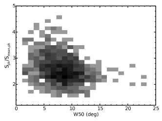
Figure 8: Number density distribution of peak flux density of bright pulses relative to their half-power width W50 for the five observations.

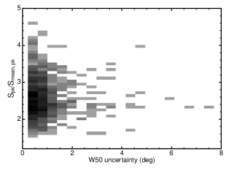
Figure 9: Number density distribution of peak flux density of bright pulses relative to the uncertainty in their half-power width W50 for the five observations.

Figure 8 shows the two-dimensional distribution of half-power pulse widths W50 versus peak flux density for PSR J1745$-$2900 and Figure 9 shows the distribution of uncertainties in the W50 measurements. Pulse widths were derived using a linear interpolation between profile data points to define the pulse phase at 50% of the pulse peak. Uncertainties in the widths were estimated by dividing the baseline rms noise level by the gradient of the profile at each side and adding the width uncertainties for each side in quadrature.

As has been observed in some other pulsars, e.g., PSR J0437$-$4715 (Jenet et al., 1998) and the Crab pulsar PSR B0531+21 (Majid et al., 2011), Figure 8 shows an anticorrelation between peak flux density and pulse width, W50, for single pulses. Figure 9 shows that, apart from a few outliers, the width uncertainty for most single pulses is a degree or less, with no strong dependence on peak intensity. Consequently, the observed larger width of weaker pulses is not due to larger uncertainties. This conclusion is reinforced by Figure 10 which shows the distribution of widths averaged over two bands of peak flux density, respectively, pulses weaker than S_pk/S_mean,pk $=$ 2.8, and greater than this value. The two distributions are well fitted by Gaussian curves and are signficantly different with mean widths of $8\aas@@fstack{\circ}6$ for weaker pulses and $7\aas@@fstack{\circ}1$ for stronger pulses. A two-sample KS test shows that the two Gaussian distributions are significantly different at the 95% confidence level.

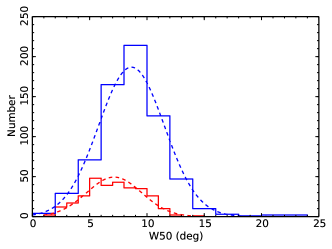
Figure 10: Distributions of the pulse width W50 of weak pulses (S_pk/S_mean,pk <2.8, blue) and strong pulses (S_pk/S_mean,pk $\geq$ 2.8, red). The dashed lines are the best-fitting Gaussian curves to each sample.

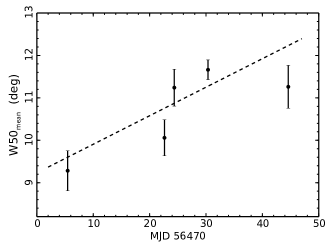
Figure 11: Full width at half maximum of mean pulse profiles observed at each epoch as a function of time (points with error bars) and the best linear fitting (dashed line) for PSR J1745$-$2900.

The time variations of the 50% pulse width of mean pulse profiles $\mathrm{W50_{mean}}$ are presented in Figure 11. Here, $\mathrm{W50_{mean}}$ is an average of half-power widths of each subintegration of a given observation. The plotted width uncertainties are simply the standard deviation of the individual values used to determine the average. The results of Lynch et al. (2015) showed that there was an apparent increase in pulse profile width between MJDs 56544 and 56594 with a fitted rate of change of $0\aas@@fstack{\circ}08\ \pm\ 0\aas@@fstack{\circ}04\ \mathrm{day^{-1}}$. Our results shown in Figure 11 are consistent with the results of Lynch et al. (2015), showing an obvious increase in W50 between MJDs 56475 and 56514. The best-fit line gives a slope of $0\aas@@fstack{\circ}07\ \pm\ 0\aas@@fstack{\circ}03\ \mathrm{day^{-1}}$.

Yan et al. (2015) reported that narrow spikes with half-power widths in the range of $0\aas@@fstack{\circ}2-0\aas@@fstack{\circ}9$ were detected from this pulsar at 8.6 GHz. Their peak flux densities were at least 10 times larger than the peak flux density of the mean pulse profile. In our results, the half-power widths of the narrowest single pulses are about $1\aas@@fstack{\circ}1$. However, their peak flux densities are no more than four times of the peak flux density of the mean pulse profile.

3.2.3 Subpulse drifting

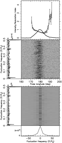
Figure 12: Results of fluctuation analysis for the PSR J1745$-$2900 observation of MJD 56475. The top panel shows the mean pulse profile (solid line) and longitude-resolved modulation index (points with error bars). The LRFS and a side panel showing the horizontally integrated power are given below this panel. Below the LRFS, the 2DFS and side panels showing horizontally (left) and vertically (bottom) integrated power are plotted.

Many pulsars show the phenomenon of subpulse drifting in which the subpulses drift in pulse phase or longitude across a sequence of single pulses (e.g. Weltevrede et al. 2006a). The subpulse drifting pattern is quasi-periodic with a characteristic spacing of the subpulses in pulse longitude (P2) and pulse number (P3). In order to investigate the variability of subpulses, we carried out an analysis of fluctuation spectra by calculating the longitude-resolved modulation index, the longitude-resolved fluctuation spectrum (LRFS) (Backer, 1970) and the two-dimensional fluctuation spectrum (2DFS) (Edwards & Stappers, 2002) for the five observations. The longitude-resolved modulation index is a measure of the amount of intensity variability at a given pulse longitude, while the LRFS and the 2DFS are used to characterize P3 and P2 respectively. For more details about the techniques of analysis, we refer to Weltevrede et al. (2006a). Figure 12 gives an example of our results based on the observation of MJD 56475. The asymmetric distribution of modulation index presented in the top panel indicates that the intensity variation is different between the leading and trailing edge of the mean pulse profile. Previously, Lynch et al. (2015) and Yan et al. (2015) searched for drifting subpulses in their observations but no evidence was found for the existence of drifting subpulses. In Figure 12, the side panels of the LRFS and 2DFS show spectral features at $P/P_{3}\ \simeq\ 0.02$ cycles per period (cpp) and $P/P_{3}\ \simeq\ 0.5$ cpp. However, these spectral features are both produced by interference because they are visible at the whole range of pulse longitude. No subpulse modulation feature can be seen in either the LRFS or the 2DFS. This confirms the results presented by Lynch et al. (2015) and Yan et al. (2015) that subpulse drifting is not detectable in PSR J1745$-$2900.

3.3 Pulse nulling

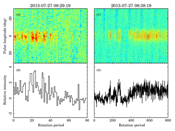
Figure 13: Pulse energy variations with time for the observation of MJD 56500 (panel (D)) and a 5-min prior observation (panel (B)) with corresponding single-pulse stacks on top (panels (A) and (C)). The start UTC times of the two observations are shown on the top of each column.

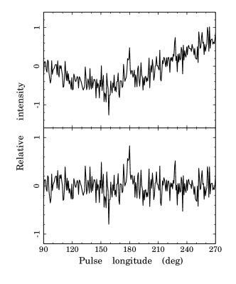
Figure 14: Mean pulse profile of null pulses between rotation period 80 and 100 in the right column of Figure 13 (upper) and the same profile after baseline fluctuation mitigation (lower).

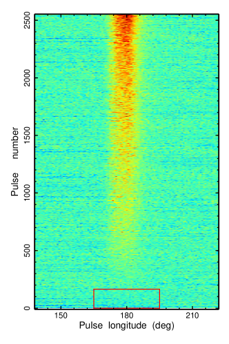
Figure 15: Arranged individual pulses in the ascending order of their on-pulse energy for the observation of MJD 56500. The null pulses can be seen towards the low energy end (inside an indicative red box).

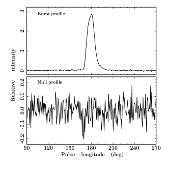
Figure 16: Mean pulse profiles of null pulses (lower) and burst pulses (upper).

Pulsar nulling is a phenomenon in which pulsed emission suddenly turns off for several pulse periods and then just as suddenly turns on (e.g. Wang et al. 2007). Nulling is relatively common in pulsars and observed mostly in longer-period pulsars. Nulling has been shown to occur in more than 100 pulsars to date (Ritchings, 1976; Rankin, 1986; Biggs, 1992; Vivekanand, 1995; Wang et al., 2007; Burke-Spolaor et al., 2012; Gajjar et al., 2012). Although the radio emission properties of magnetars are similar to those of the normal pulsars in several respects (Kramer et al., 2007), nulling has not been reported in magnetars before. Visual inspection of Figure 1 shows that there are several apparent nulls in the observation of MJD 56500. The pulse energy distribution shown in Figure 7 has a small secondary peak at $E/\langle E\rangle=0$, also suggesting pulse nulling or weak modes in PSR J1745$-$2900.

The pulse energy variations with time are presented in Figure 13 for the observation of MJD 56500 (right column) and a short 5-min observation 9 minutes earlier (left column). The upper panels show the color-scale plots of single-pulse intensities for the two observations. Corresponding pulse energy variations are shown in the lower panels. As we can see in panels (A) and (B), the pulsar fades out after rotation period 44. Panel (C) shows that there are obvious pulse cessations in period ranges of $\sim$1-150, 180-220, 230-250 and 300-370. These cessations look very like pulsar nulling. Panel (D) shows clearly that the pulse energy drops to zero several times before the rotation period 370 and return to normal after then. This is consistent with the nulling phenomenon observed in normal pulsars. Since the gap between the UTC 08:29:19 observation and the UTC 08:38:19 observation is about four minutes, panels (B) and (D) suggest that the nulling event lasted about 30 minutes (from rotation period 44 in panel (B) to rotation period 370 in panel (D)). Of course it is also possible that the pulsed emission switched on again during the observation gap.

Weak emission was detected in PSR B0826$-$34 during an apparent null phase (Esamdin et al., 2005). We therefore investigated whether the apparent nulls seen in PSR J1745$-$2900 are real nulls or weak modes by forming null-phase pulse profile by averaging the pulses in the null state. For simplicity, we chose pulses in the most apparent null state, i.e., pulses between rotation period 80 and 100 in Figure 13, to form the mean pulse profile. The profile obtained from these null pulses is shown in the upper panel of Figure 14. Baseline fluctuations are present in our data. These can arise from receiver fluctuations, atmospheric fluctuations or they may be intrinsic to the pulsar. Similar baseline fluctuations were seen by Lynch et al. (2015) and attributed by them to changes in atmospheric opacity. Simultaneous observations at multiple telescopes and frequencies would help to establish the origin of these fluctuations. We tried to mitigate their effect in our data by fitting a sine function to the baseline and subtracting it from the data. The resulted profile is given in the lower panel. Surprisingly, the average profile of the null pulses shows a clear detection of the pulse profile. It is therefore important to know if the weak emission profile arises from bright but rare single pulses, or if it is a steady weak emission.

Following Gajjar et al. (2017), to investigate this we arranged all pulses from the MJD 56500 observation in ascending order of their on-pulse energy as shown in Figure 15. If the weak emission profile of null pulses originates from a few single pulses, there should be no evidence of any emission when we just average several null pulses with lowest on-pulse energy. On the contrary, if the weak emission profile originates from intrinsic weak emission, there should be evidence of emission even if we only average a few weak null pulses. We formed mean pulse profiles by averaging different numbers of the weakest null pulses as indicated by the box at the bottom of Figure 15. The upper edge of the box was moved toward the high-energy end until the mean profile for pulses inside the box show a significant emission profile (peak S/N $>3\sigma$). This level was used to divide all pulses into two groups with pulses outside this box marked as burst pulses and the pulses inside the box marked as null pulses.

After this separation, the average profiles obtained from the null pulses and the burst pulses are presented in Figure 16. The mean pulse profile of null pulses in the lower panel does not show any significant emission component. This suggests that the weak emission profile shown in Figure 14 arises from bright but rare single pulses instead of a steady weak emission. Hence we can conclude that the apparent null states observed on MJD 56500 are real nulls rather than being a weak-emission mode.

4 Discussion and conclusions

We have presented the mean pulse profile and single-pulse properties of PSR J1745$-$2900 at 3.1 GHz by analyzing five observations with high S/N made at epochs between 2013 July and August. The data were downloaded from the Parkes Pulsar Data Archive.

A stable radio state is not often seen in radio-emitting magnetars. During the stable state, the magnetar acts more like a normal pulsar, in that both the radio pulse profile shape and flux density are stable. The similarity of the mean pulse profile shape of the five observations indicates that the pulsar was in a stable state between MJDs 56475 and 56514. As the observations analyzed here occurred before the GBT observations reported by Lynch et al. (2015), the observations extend the stable state of this pulsar from 5.5 months to 6.8 months.

In spite of the large DM, interstellar scattering is not a dominating effect for the mean pulse profile of PSR J1745$-$2900 at 3.1 GHz with the expected scattering timescale being about 18 ms or $1\aas@@fstack{\circ}7$ of pulse phase (Spitler et al., 2014). We detected a linear variation with a slope of $0\aas@@fstack{\circ}07\ \pm\ 0\aas@@fstack{\circ}03\ \mathrm{day^{-1}}$ in the pulse width of mean pulse profiles between MJDs 56544 and 56594, which confirms and extends the pulse width variations presented by Lynch et al. (2015).

Lynch et al. (2015) noted that the pulse profile prior to their GBT observations was single peaked while the pulse profile in the stable state of their observations was double peaked. Similar to the pulse width evolution, they found that the component separation increased with time during their observations, with a value of $5\aas@@fstack{\circ}5$ ($\sim$57 ms) at the time of their first observation on MJD 56515. The last Parkes observation was just one day earlier at MJD 56514 and, for all of our observations, the pulse profile was single-peaked (Figure 1). Since the Spitler et al. (2014) 3.2 GHz observations were almost coincident with those at Parkes, it is unlikely that the single-peaked Parkes profiles result from scatter broadening. In view of the near coincidence in time of the last Parkes observation and the first GBT observation, it seems more probable that at this time there was an evolution in frequency of the shape of the mean pulse profile, with the components becoming better defined at higher frequencies.

Single-pulse observations of some pulsars, for example, PSR B0656+14 (Weltevrede et al., 2006b), PSR B1839$-$04 (Weltevrede, 2016) and PSR J1713+0747 (Liu et al., 2016), showed that the observed on-pulse energy distribution can be modelled by convolving an intrinsic distribution with the observed noise distribution. With the same analysis, we found that the intrinsic pulse energy distribution of PSR J1745$-$2900 at 3.1 GHz is well described by a log-normal distribution. We found an anticorrelation between peak flux density of single pulses and their 50% width similar to those observed in the millisecond pulsar PSR J0437$-$4715 (Jenet et al., 1998) and the Crab pulsar PSR B0531+21 (Majid et al., 2011). Stronger pulses have a mean width of $7\aas@@fstack{\circ}1$ and for weaker pulses the mean width is $8\aas@@fstack{\circ}6$. We showed that the pulse width distributions for strong and weak single pulses are significantly different at the 95% confidence level. Consistent with the results presented by Lynch et al. (2015) and Yan et al. (2015), giant pulses and subpulse drifting were not detected in the five observations for J1745$-$2900 at 3.1 GHz.

Besides the long time-scale evolution of the mean pulse profile, PSR J1745$-$2900 also shows short time-scale pulse shape variations. By forming short sub-integrations, we found evidence for mode changing on timescales of several minutes. One mode has two clear overlapping components whereas the other only shows a broad single component.

We detected pulsar nulling in PSR J1745$-$2900. In the observation of MJD 56500, the pulse energy drops to zero several times then return to the normal level. We could find no evidence for instrumental problems that could cause apparent nulls and neither diffractive nor refractive scintillation can account for the variations. The observing band covers many diffractive bands and the timescale for refractive scintillation is of the order years (Bower et al., 2015; Pennucci et al., 2015). Summing of data within null regions reveals a weak pulse, but we believe that this results from an occasional strong pulse rather than indicating that the null is a weak emission mode.

In some respects, the radio emission of magnetars is different from that of normal radio pulsars. For magnetars, the radio emission is transient, the radio flux density and the pulse profile are highly variable, and the radio spectrum is relatively flat. The radio emission of XTE J1810$-$197 (PSR J1809$-$1943) is always extremely variable, its radio flux density and pulse shape showed dramatic changes on time-scales ranging from minutes to weeks (Camilo et al., 2007a; Kramer et al., 2007; Lazaridis et al., 2008; Camilo et al., 2016). The flux density of PSR J1622$-$4950 varies up to a factor of $\sim$10 within a few days and the observed pulse shapes of PSR J1622$-$4950 changes significantly from day to day (Levin et al., 2010, 2012). PSR J1550$-$5418 also showed variations in pulse profile shape and flux density, with the flux density varying by factors up to $\sim$50$\%$ on timescales of a few days (Camilo et al., 2008). These variations observed in radio-emitting magnetars are intrinsic to the pulsar and may be related to changes in magnetospheric plasma densities and/or currents. Based on the differences between magnetar radio emission and normal pulsar radio emission, it has been proposed that the radio emission of magnetars is powered by magnetic field decay instead of by rotation (Tong et al., 2013). However, in other respects the radio emission from the two classes of pulsar is similar. For example, the pulse polarization properties of magnetars are similar to those of other pulsars (e.g., Camilo et al., 2007a; Eatough et al., 2013). The presence of mode changing and pulsar nulling in the GC magnetar PSR J1745$-$2900 gives further support to the idea that the radio emission mechanism is bascially the same in magnetars and normal pulsars.

References

- Backer (1970) Backer D. C., 1970, Nature, 227, 692
- Biggs (1992) Biggs J. D., 1992, ApJ, 394, 574
- Bower et al. (2014) Bower G. C., et al., 2014, ApJ, 780, L2
- Bower et al. (2015) Bower G. C., et al., 2015, ApJ, 798, 120
- Burke-Spolaor et al. (2012) Burke-Spolaor S., et al., 2012, MNRAS, 423, 1351
- Camilo et al. (2006) Camilo F., Ransom S. M., Halpern J. P., Reynolds J., Helfand D. J., Zimmerman N., Sarkissian J., 2006, Nature, 442, 892
- Camilo et al. (2007a) Camilo F., Reynolds J., Johnston S., Halpern J. P., Ransom S. M., van Straten W., 2007a, ApJ, 659, L37
- Camilo et al. (2007b) Camilo F., Ransom S. M., Halpern J. P., Reynolds J., 2007b, ApJ, 666, L93
- Camilo et al. (2008) Camilo F., Reynolds J., Johnston S., Halpern J. P., Ransom S. M., 2008, ApJ, 679, 681
- Camilo et al. (2016) Camilo F., et al., 2016, ApJ, 820, 110
- Duncan & Thompson (1992) Duncan R. C., Thompson C., 1992, ApJ, 392, L9
- Eatough et al. (2013) Eatough R. P., et al., 2013, Nature, 501, 391
- Edwards & Stappers (2002) Edwards R. T., Stappers B. W., 2002, A&A, 393, 733
- Esamdin et al. (2005) Esamdin A., Lyne A. G., Graham-Smith F., Kramer M., Manchester R. N., Wu X., 2005, MNRAS, 356, 59
- Esamdin et al. (2012) Esamdin A., Abdurixit D., Manchester R. N., Niu H. B., 2012, ApJ, 759, L3
- Gajjar et al. (2012) Gajjar V., Joshi B. C., Kramer M., 2012, MNRAS, 424, 1197
- Gajjar et al. (2017) Gajjar V., Yuan J. P., Yuen R., Wen Z. G., Liu Z. Y., Wang N., 2017, ApJ, 850, 173
- Hobbs et al. (2011) Hobbs G., et al., 2011, PASA, 28, 202
- Hotan et al. (2004) Hotan A. W., van Straten W., Manchester R. N., 2004, PASA, 21, 302
- Jenet et al. (1998) Jenet F., Anderson S., Kaspi V., Prince T., Unwin S., 1998, ApJ, 498, 365
- Kennea et al. (2013) Kennea J. A., et al., 2013, ApJ, 770, L24
- Kramer et al. (2007) Kramer M., Stappers B. W., Jessner A., Lyne A. G., Jordan C. A., 2007, MNRAS, 377, 107
- Krishnakumar et al. (2015) Krishnakumar M. A., Mitra D., Naidu A., Joshi B. C., Manoharan P. K., 2015, ApJ, 804, 23
- Lazaridis et al. (2008) Lazaridis K., Jessner A., Kramer M., Stappers B. W., Lyne A. G., Jordan C. A., Serylak M., Zensus J. A., 2008, MNRAS, 390, 839
- Levin et al. (2010) Levin L., et al., 2010, ApJ, 721, L33
- Levin et al. (2012) Levin L., et al., 2012, MNRAS, 422, 2489
- Liu et al. (2015) Liu K., et al., 2015, MNRAS, 449, 1158
- Liu et al. (2016) Liu K., et al., 2016, MNRAS, 463, 3239
- Lorimer & Kramer (2005) Lorimer D. R., Kramer M., 2005, Handbook of Pulsar Astronomy. Cambridge University Press
- Lynch et al. (2015) Lynch R. S., Archibald R. F., Kaspi V. M., Scholz P., 2015, ApJ, 806, 266
- Majid et al. (2011) Majid W. A., Naudet C. J., Lowe S. T., Kuiper T. B. H., 2011, ApJ, 741, 53
- Mori et al. (2013) Mori K., et al., 2013, ApJ, 770, L23
- Olausen & Kaspi (2014) Olausen S. A., Kaspi V. M., 2014, ApJS, 212, 6
- Pennucci et al. (2015) Pennucci T. T., et al., 2015, ApJ, 808, 81
- Rankin (1986) Rankin J. M., 1986, ApJ, 301, 901
- Rea et al. (2010) Rea N., et al., 2010, Science, 330, 944
- Rea et al. (2012) Rea N., et al., 2012, ApJ, 754, 27
- Rea et al. (2013) Rea N., et al., 2013, ApJ, 775, L34
- Rea et al. (2014) Rea N., Viganò D., Israel G. L., Pons J. A., Torres D. F., 2014, ApJ, 781, L17
- Ritchings (1976) Ritchings R. T., 1976, MNRAS, 176, 249
- Shannon & Johnston (2013) Shannon R. M., Johnston S., 2013, MNRAS, 435, L29
- Spitler et al. (2014) Spitler L. G., et al., 2014, ApJ, 780, L3
- Thompson & Duncan (1995) Thompson C., Duncan R. C., 1995, MNRAS, 275, 255
- Thompson & Duncan (1996) Thompson C., Duncan R. C., 1996, ApJ, 473, 322
- Tong et al. (2013) Tong H., Yuan J.-P., Liu Z.-Y., 2013, RAA, 13, 835
- Torne et al. (2015) Torne P., et al., 2015, MNRAS, 451, L50
- Torne et al. (2017) Torne P., et al., 2017, MNRAS, 465, 242
- van Straten & Bailes (2011) van Straten W., Bailes M., 2011, PASA, 28, 1
- Vivekanand (1995) Vivekanand M., 1995, MNRAS, 274, 785
- Wang et al. (2007) Wang N., Manchester R. N., Johnston S., 2007, MNRAS, 377, 1383
- Weltevrede (2016) Weltevrede P., 2016, A&A, 590, A109
- Weltevrede et al. (2006a) Weltevrede P., Edwards R. T., Stappers B. W., 2006a, A&A, 445, 243
- Weltevrede et al. (2006b) Weltevrede P., Wright G. A. E., Stappers B. W., Rankin J. M., 2006b, A&A, 458, 269
- Yan et al. (2015) Yan Z., et al., 2015, ApJ, 814, 5
- Yao et al. (2017) Yao J. M., Manchester R. N., Wang N., 2017, ApJ, 835, 29