STATISTICAL COMPLEXITY WITHOUT EXPLICIT REFERENCE TO UNDERLYING PROBABILITIES

Abstract

We show that extremely simple systems of a not too large number of particles can be simultaneously thermally stable and complex. To such an end, we extend the statistical complexity’s notion to simple configurations of non-interacting particles, without appeal to probabilities, and discuss configurational properties.

Keywords: Disequilibrium without probabilities, Statistical complexity, Disequilibrium.

I Introduction

Examples of collective phenomena which can emerge from real-world complex systems include traffic congestion, financial market crashes, wars, and epidemics. They do not involve $10^{24}$ objects or agents but rather thousands, so that canonical ensemble considerations may not be adequate while micro-canonical (MC) ones may apply. MC dealings do not involve probabilities and will be the focus of our interest here.

Now, to be aware of a system’s degree of randomness is not enough for an adequate insight into the extant correlation structures. One may try to search for a way to be in a position to discern the relations among a system’s components by recourse to a specific quantifier, mimicking the manner in which entropy $S$ describes disorder. Two extreme situations may be encountered: (a) perfect order or (b) maximal randomness. In these cases strong correlations do not exist LMC . In between, variegated degrees of correlation are possible and we would wish that the above mentioned quantifier would quantify them. We may call it a “complexity”. How is one to represent it? The answer is not easily found. Famously, Seth Lloyd enumerated some 40 manners of defining this “complexity”, none of them optimal.

A system may be regarded as complex, obviously, when it does not fit simple patterns, as in the case of either (I) a perfect crystal or (II) the isolated ideal gas. These are good examples of simplicity, or, alternatively, instances of null complexity. In a crystal, the information, or negentropy ($-S$) stored is minimal. A few parameters suffice for a good description. On the contrary, the ideal gas is completely disordered, with any of its accessible states endowed with the same probability, that exhibits maximum entropy. Systems (I) and (II) are extreme in the scale of order/information, which implies that complexity cannot be cast in terms of order or information. In Ref. LMC the authors advance a measure of complexity by employing some kind of distance to the maximum entropy situation, called disequilibrium (D) LRuiz2001 . $D$ yields a notion of hierarchy that would be different from zero if there are privileged states among those accessible ones. $D$ would be maximal for the perfect crystal and vanish for the ideal gas. For the entropy (S), things are exactly reversed, being minimal for the crystal and maximal for the ideal gas. Accordingly, L. Ruiz, Mancini, and Calvet (LMC) LMC advanced, in what constituted a great leap forward, a statistical complexity measure $C$ of the form

$$C=DS,$$ (1)

that is an interesting functional of the probability distributions that does grasp correlations in the way that entropy captures randomness LMC . The quantity $D$ measures (in probability space) the distance from i) the prevailing probability distribution to ii) the uniform probability and it reveals the amount of structural details LMC ; cuatro . For a system of $N-$particles one has

$$D=\sum_{i=1}^{N}\,\left(p_{i}-\frac{1}{N}\right)^{2}.$$ (2)

Here ${p_{1},p_{2},\ldots,p_{N}}$ are the individual normalized probabilities ($\sum_{i=1}^{N}\,p_{i}=1$) LMC . $D$ attains the maximum value for a fully ordered state and vanishes in the case of completely disordered states or equiprobable states. Moreover, LMC’s statistical complexity also it individualize and quantify the bequeath of Boltzmann’s entropy (or information $S=-\sum_{i=1}^{N}\,p_{i}\ln p_{i}$).

This proposal received considerable attention and great interest LMC ; MPR ; lmc1 ; lmc11 ; lmc2 ; lmc22 ; lmc3 ; cuatro , being applied in different scenarios for both the canonical and grand canonical ensembles. It is obvious that $C$ vanishes in the (opposite) simple cases (I) and (II) above.

We will here focus attention, for the first time as far as we know, on a $C-$scenario devoid of both i) probabilities and ii) interacting particles. We show that quantifiers like $S$, $D$, and $C$ can be defined and yield new information regarding the behavior of the simplest conceivable system: two level systems of $N$ identical, independent particles. Its simplicity notwithstanding, such systems do exhibit complex behavior and can attain internal stability. It has been forcefully argued that binary decision problems provide the perfect illustration of complexity three , while presenting workers in the field with an exceedingly challenging problem that,as far as we know, no satisfactory mathematics to account for it three . Here we consider binary decisions as those of a particle regarding to whether to occupy or not one of the model’s two levels. We will obtain intriguing insights.

The paper is organized as follows. In Section II we introduce relevant concepts related to the two-level model, as well as the motivation of our research. In Section III we define the quantities $C$ and $D$ mentioned above without using probabilities. This constitutes a crucial issue of endeavor. Section IV is devoted to the study of the free energy $F$, indispensable to establish the existence of regions of thermal stability. Useful relations between $C$ and $D$, together with the specific heat, are obtained in Section V. Possible generalizations are outlined in Section VI. Finally, we draw conclusions in Section VII.

II Two level system

We begin by noting that an early complexity-related effort on this theme is due to L. Ruiz lr2 by considering a laser of two levels of energy and appealing to a normal probability distribution in the canonical ensemble. This valuable work is totally unrelated to the present one, though.Let us consider a system with $N$ indistinguishable particles with energy $E$ miranda . Each particle can be found in two possible states of energy (in suitable units) $0$ and $1$, respectively, with $M$ particles in the latter level and $N-M$ in the former. In such a scenario, the system’s configuration is uniquely characterized by the pair ($N,M$) and has a state-degeneracy given by kelly ; kittel ; ramsey

$$\Omega(M,N)=\frac{N!}{(N-M)!M!},$$ (3)

with, obviously, $M=E$. Accordingly, following the celebrated equation $S=\ln{\Omega}$ engraved in L. Boltzmann’s tomb at Vienna’s cemetery, the entropy obtained from Eq. (3) is (in Boltzmann’s constant $k_{B}$-units)

$$S=\ln\left(\frac{N!}{(N-M)!M!}\right).$$ (4)

The general aspect of this entropy is illustrated by Fig. 1 for $N=50$, not a novel graph that we include here for pedagogical purposes.

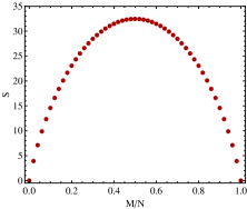
Figure 1: Entropy $S$ as a function of $M/N$ for $N=50$ in which $M/N$ runs between 0 and $1$.

We deal with a collection of configurations (we may speak of micro-canonical configurations) uniquely characterized by the pair ($N,M$). All relevant physical quantities are determined by these pairs. For each of them, i.e., for each possible configuration, we have fixed values of temperature $T$, disequilibrium $D$, entropy $S$, statistical complexity $C$, and free energy $F$. The pertinent relationships will be given below in $N,\,M$-terms. This is a particular instance of a much more general one in which the temperature of a system affects the configurations adopted by that system, and consequently one would expect to be able to calculate the temperature from configurational information configurat .

In this work, we are going to compare amongst these configurations and try to discern patterns. Note that, since for each configuration $T$ is effectively fixed, the free energy concept does make sense. In other words, this paper is a statistical study of the variables $N$ and $M$ over a collection of ($N,M$) configurations.

II.1 Temperatures

The temperature of the system as a function of $M$, $N$ is obtained from the thermodynamical entropy (4). Thus, in this case, one has Huang

$$\frac{1}{T}=\frac{\partial S(N,M)}{\partial M}.$$ (5)

Since the energy is a discrete quantity, for not too large systems, the derivatives are replaced by finite differences and Eq. (5) becomes miranda

$$\frac{1}{T(N,M)}=\frac{S(N,M)-S(N,M-1)}{M-(M-1)}=S(N,M)-S(N,M-1).$$ (6)

Replacing Eq. (4) into Eq. (6), one obtains miranda

$$\frac{1}{T}=\ln\left(\frac{N}{M}-1+\frac{1}{M}\right),$$ (7)

entailing that $T$ diverges for $M=(N+1)/2$. An illustration, we depict in Fig. 2 the temperature $T$ given by Eq. (7) for $N=50$. By inverting the above relation we find

$$M(N,T)=\frac{N+1}{1+e^{1/T}},$$ (8)

yielding $M(N,T)=E(N,T)$ as a function of $T$.

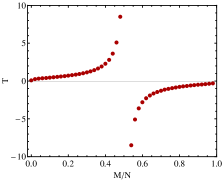
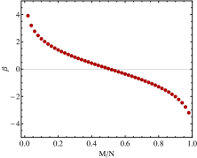
(a)  (b)

Figure 2: (a): Temperature $T$ versus $M/N$ for $N=50$. A divergence takes place at $M/N=0.51$. (b): Inverse temperature $\beta=1/T$ versus $M/N$ for $N=50$.

II.2 Motivation

Let us reiterate: from Eq. (7), we observe that $T\geq 0$ whenever $N/M-1+1/M>1$, that is, $M\leq(N+1)/2$. Otherwise, $T<0$ implies that $M>(N+1)/2$. Moreover, $T$ diverges when $N/M-1+1/M=1$ implying that $M=(N+1)/2$. It is well known that negative temperatures always arise if there is an upper bound to the system’s energy. States with negative temperature are actually hotter than states with positive temperature kelly ; kittel ; ramsey . The $T-$divergence is the origin of the interesting physics to be described below. Actually, Fig. 2 constitutes our motivation for investigating the statistical complexity in this context. It is clear that the above mentioned divergence may justify hopes of finding in it the source of complex behavior. In particular, note that, trivially, $\beta=1/T$ behaves as an order parameter glass in the following sense: let us call “symmetric” (occupationally symmetric) that state with roughly the same number of particles in each of the two levels. $\beta$ is zero in the high temperature, or symmetric, state, but at low temperatures, when this symmetry is “broken”, it takes on a nonzero value glass . The novel point here is that we will show below that LMC’s disequilibrium $D$ is also an order parameter in this peculiar sense.

On a different vein, and as stated in the Introduction, in this paper we deal, in essence, with a collection of micro-canonical configurations. Why to look at complexity in such a setting? Because it seems unlikely that theories which need to assume very large numbers of objects (so that appeal to the canonical ensemble makes sense) may represent everyday complex systems, where the numbers involved are typically less than a thousand, or even a hundred three . For instance, in a financial market the number $N_{P}$ of people who actually have enough economic clout to “move” the market is relatively small, and it is this $N_{P}$ which should feature in any realistic model of the market three . Thus, micro-canonical modeling of complexity is indeed reasonable and does not involve probabilities.

III Defining disequilibrium and statistical complexity without an underlying probability distribution

This is the crucial issue. Once we have an adequate “probability-less” $D-$version everything follows smoothly. Given $N$, we have a collection of $M+1$ (different) possible energy-configurations. Elementary combinatorial arguments show that the configuration of maximum entropy (ME) is that of the pair $(N,N/2)$ if $N$ is even. For $N-$odd, ME is attained, with equal values, at $M=N/2\pm 1/2$.

LMC defined $D$ as a distance in probability space: that to the uniform distribution (UD). We work here in a scenario devoid of probabilities. What to do? Noting that the UD is the maximum entropy ME-distribution, the judicious $D-$choice is then the following: the disequilibrium $D$ of the configuration $(N,M)$ is to be properly defined as a kind of “distance” to the ME configuration (in configuration space). We choose, given the ME value $S_{max}$,

$$D(N,M)=1-\frac{S(N,M)}{S_{max}(N,M)},$$ (9)

where $S_{max}(N,M)=S(N,N/2)=\ln(N!/(N/2)!^{2})$. It vanishes for $S=S_{max}$ and is maximal for $S=0$, as one should expect. The corresponding analytic expression is

$$D(N,M)=\frac{\ln\left(\frac{(N-M)!M!}{(N/2)!^{2}}\right)}{\ln\left(\frac{N!}{(N/2)!^{2}}\right)}.$$ (10)

According to (1), we have now a probability-less LMC complexity given by

$$C(N,M)=D(N,M)S(N,M).$$ (11)

The adequacy of our $D-$definition could be assessed by comparing it to an orthodox LMC one that uses a suitable probability distribution. This is the goal of Fig. 3, that compares, for $N=50$, our $D$ versus $M/N$ with the orthodox LMC disequilibrium for a surrogate Boltzmann-like exponential distribution (BEP), with good agreement. This surrogate BEP is, for a given $N$, of the form

$$P_{B}=\exp{(-E_{M}/T_{M})}/Z;\,\,\,Z=\sum_{M}\,\exp{(-E_{M}/T_{M})},$$ (12)

where $T_{M}$ is the temperature of the $(N,M)$ configuration. Of course, a “true” Boltzmann distribution has a common $T$ for all $M$. We use $P_{B}$ so as to construct an orthodox LMC-$D$ and, by comparison, validate the reasonability of our probability-less $D$-definition. Beyond this role, we suggest that $P_{B}$ might arouse some interest by itself, though. We remind the reader that the true Boltzmann distribution exhibits the appearance

$$P_{B}(M)=\exp{(-E_{M}/T)}/Z;\,\,\,Z=\sum_{M}\,\exp{(-E_{M}/T)},$$ (13)

with an entropy $S_{B}$

$$S=-\sum_{M}P_{B}(M)\ln{P_{B}(M)},$$ (14)

and a disequilibrium $D$ equal to (see (2))

$$D=\sum_{M}[P_{B}(M)-(1/M)]^{2}.$$ (15)

The complexity $C$ is then usually evaluated using Eq. (1). Comparing (12) with (13) we see that our surrogate distribution is just a Boltzmann probability distribution with an $M-$dependent temperature.

Also, note that our $D$ is zero at very high temperatures (the symmetric state defined in Subsection II.2), and grows as the temperature descends, behaving thus like an order parameter glass and becoming then a thermodynamic variable glass .

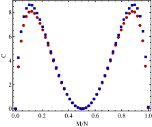
(a)  (b)

Figure 3: (a): Disequilibrium $D$ as a function of $M/N$ for the surrogate probabilistic distribution (blue square) of Eq. (12), compared to this paper’s definition (red circle) for $N=50$. (b): Same as Fig. (a) but for the statistical complexity $C$. In this case, the maxima are in $M/N=6/50$ and $M/N=44/50$.

Also, we see that $C$ vanishes for maximum entropy and for zero entropy, as it should. It also exhibits two peaks. As stated above in Subsection II.2, $D$ plays the role of an order parameter in the sense therein explained. Accordingly, LMC’s statistical complexity becomes the product of two thermodynamic variables, something that, we believe, has not been remarked before. Moreover, we encounter complexity peaks for very small values of $N$. Indeed, this happens already for $N=3$, which brings to mind the title of three : Two’s Company, Three is Complexity. In order to ascertain the $C-$peaks’ significance we turn next to the free energy $F$. We will see that only the first maximum is physically relevant.

IV The free energy $F$

This is an essential quantity which is defined, for $E=M$ (because the lowest of our two levels has zero energy), as

$$F(N,M)=M-TS(N,M).$$ (16)

The important point here is that $\mathrm{d}^{2}F/\mathrm{d}T^{2}$ should be $<0$ for thermal stability callen (Appendix G, Eqs. G2, G7, G8, and G9). Explicitly, one finds in this celebrated text-book that

$$\frac{\mathrm{d}^{2}F}{\mathrm{d}T^{2}}=-\frac{C_{h}}{T},$$ (17)

with $C_{h}$ standing for the specific heat, a positive quantity (except for gravitational systems lynden ). Thus, in our regions of positive temperature, $\mathrm{d}^{2}F/\mathrm{d}T^{2}$ is negative. Additionally, we observe that for the two-level system, $\mathcal{C}_{h}$ is given by the discrete relation miranda

$$\mathcal{C}_{h}(N,M)=\frac{1}{T(N,M)-T(N,M-1)}.$$ (18)

If we replace this into Eq. (17) we arrive at

$$\frac{\mathrm{d}^{2}F}{\mathrm{d}T^{2}}=-\frac{1}{T(N,M)[T(N,M)-T(N,M-1)]}.$$ (19)

In Fig. 4 we plot 1) $F$ vs. $M/N$ (left) and 2) $\mathrm{d}^{2}F/\mathrm{d}T^{2}$ (given by Eq. (19)) vs. $M/N$ (right). This second derivative is $<0$ only in the region of the first of the two complexity maxima, which becomes then the only physically relevant one. Our recurrent divergence reappears for $F$ at the proper $M/N$ place. A $\mathrm{d}^{2}F/\mathrm{d}T^{2}$-minimum is attained in the vicinity of $M/N=0.1$, where one finds the first complexity maximum. One might conjecture that, if $F<0$, the system could be regarded as “bounded”, since one would need to provide energy so as to “break it up” desloge . On such a vein, one could guess that this should spontaneously happen for $F>0$. The maximum complexity and the maximum stability take place at roughly the same $M/N$-value. The most complex configuration is the most stable one. It is attained at $T>0$ and $F<0$.

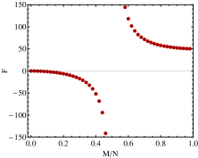
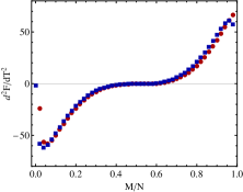
(a)  (b)

Figure 4: (a): Free energy $F$ as a function of $M/N$ for $N=50$. Of course, $F$ diverges at the same place at which $T$ does. (b): second derivative of the free energy $F$ with respect to temperature $T$ as a function of  $M/N$ for $N=50$. The blue line corresponds to $\mathrm{d}^{2}F/\mathrm{d}T^{2}$ for the two-level system using the surrogate distribution (12) in constructing $F$.

The specific heat $\mathcal{C}_{h}$ vs. $M/N$, is plotted in Fig. 5 together with its version according to the surrogate probability distribution of Eq. (12). Nest, we depict $C$ and $\mathrm{d}^{2}F/\mathrm{d}T^{2}$ versus $M/N$ in Fig. 6, that exhibits the notable fact that maximum statistical complexity obtains at the same $M/N$-location at which one has maximal thermal stability.

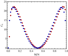
Figure 5: Our version of the specific heat $\mathcal{C}_{h}$ as a function of $M/N$ for $N=50$ ( red). Blue squares: LMC $\mathcal{C}_{h}$, using the surrogate distribution (12).

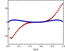
Figure 6: $C$ (blue square) and $\mathrm{d}^{2}F/\mathrm{d}T^{2}$ (red circle) versus $M/N$ for $N=50$.

In addition, we also add here in Fig. 7 a plot depicting the dependence on $N$ of the $M/N$-location of three important quantities: 1) $C$, 2) $\mathcal{C}_{h}$, and 3) $\mathrm{d}^{2}F/\mathrm{d}T^{2}$. The last two refer to the most stable situation, while the first does so for the complexity-maximum. The three locations are close neighbors. Also, maximum complexity and stability are attained at the same location for $N=3$, which brings to mind the book-title in Ref. three .

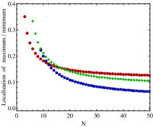
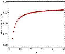
(a)  (b)

Figure 7: (a): Plot of $M/N-$location of the maximum value of $C$ (red circle), minimum of $\mathrm{d}^{2}F/\mathrm{d}T^{2}$ (blue square), and maximum of $\mathcal{C}_{h}$ (green diamond) as a function of $N$ that runs between 3 and 50. (b): Maximum of $C/N$ versus $N$ between 3 and 50. We see that the maximal complexity per particle is of about $0.17$ for most of the $N-$range.

In order to calculate the maximum of $C$ for $N$ between 2 to 200 particles, we look at the discrete derivative of $C$ respect to $M$ miranda , i.e.,

$$\frac{\mathrm{d}C(N,M)}{\mathrm{d}M}=C(N,M)-C(N,M-1).$$ (20)

The extremes are attained when $\mathrm{d}C/\mathrm{d}M=0$. Therefore, employing definitions (6), (9), and (11), we obtain

$$S_{max}(N,M)=T(N,M)\left[S^{2}(N,M)-S^{2}(N,M-1)\right].$$ (21)

The above equation is solved numerically to find that $M$ for which $C/N$ is maximum. The results are depicted in Fig. 7.

The asymptotic behavior is found as follows. First, for $N\gg 200$, we calculate, for fixed $N$, the first derivative of $C$ with respect to $M$. One has

$$\frac{\mathrm{d}C}{\mathrm{d}M}=\left(1-\frac{2S}{S_{max}}\right)\frac{\mathrm{d}S}{\mathrm{d}M}.$$ (22)

We see that $\mathrm{d}C/\mathrm{d}M$ is zero provided that $1-2S/S_{max}=0$ plus $\mathrm{d}S/\mathrm{d}M\neq 0$. Such conditions lead to $S=S_{max}/2$, so that, replacing this into Eq. (11), and using Stirling’s approximation ($\ln N!\approx N\ln N-N$), we immediately find

$$\frac{C_{max}}{N}\approx\frac{\ln 2}{4}=0.1732.$$ (23)

For $N>200$, $C$ grows linearly with $N$. One might wish to see this result as an extremely simple instance of Anderson’s more is different apothegm anderson .

V Relations amongst $T$, $C$, $D$, and the specific heat

We begin this section making use of Eq. (9), from which we obtain the entropy as

$$S=S_{max}\,(1-D).$$ (24)

Thus, using the relation (24), the specific heat adopts the appearance

$$\mathcal{C}_{h}=T\frac{\mathrm{d}S}{\mathrm{d}T}=-S_{max}T\,\frac{\mathrm{d}D}{\mathrm{d}T}.$$ (25)

Taking into account that the statistical complexity is $C=DS$, we also get

$$\frac{\mathrm{d}C}{\mathrm{d}T}=S_{max}(1-2D)\,\frac{\mathrm{d}D}{\mathrm{d}T}.$$ (26)

Considering Eqs. (25) and (26), we find a crucial relation between $\mathcal{C}_{h}$, $D$, and $C$, namely,

$$\mathcal{C}_{h}=\left(\frac{T}{2D-1}\right)\frac{\mathrm{d}C}{\mathrm{d}T}.$$ (27)

Stability of a thermodynamic systems requires $\mathcal{C}_{h}\geq 0$ so that Eq. (17) tells us that stability is attained when $\mathrm{d}^{2}F/\mathrm{d}T^{2}\leq 0$ at $T\geq 0$ –see discussion in subsection IV. To verify the stability criteria we show, in Fig. 8, the behavior of the quantity $2D-1$ as a function of temperature $T$. There, we see that $2D-1\geq-1$ for all $T$. Thus, in order to guarantee stability, two possibilities arise we are: $2D-1>0\,\wedge$ $\mathrm{d}C/\mathrm{d}T\geq 0$, and $2D-1<0\,\wedge$ $\mathrm{d}C/\mathrm{d}T<0$. Since we are here interested in the region $T>0$, this implies that $0\leq M/N\leq 0.5$.

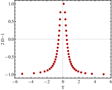
Figure 8: $2D-1$ as a function of temperature $T$ for $N=50$.

In addition, according to Eq. (25), stability is also attained when $\mathrm{d}D/\mathrm{d}T\leq 0$ implying that, by Eq. (24), $\mathrm{d}S/\mathrm{d}T\geq 0$, as it should. Summing up, the stability criterion for this simple system, which we illustrate in Fig. 9, is

$$\mathcal{C}_{h}\geq 0\Leftrightarrow\mathrm{d}^{2}F/\mathrm{d}T^{2}\leq 0\Leftrightarrow\mathrm{d}C/\mathrm{d}T\leq 0\,\,\,\textrm{for}\,\,\,0\leq M/N\leq 0.5.$$ (28)

It is clear that the complexity should diminish as the temperature grows, as expressed by the relation $\mathrm{d}C/\mathrm{d}T\leq 0$. The coherence of our overall picture can be appreciated once again. This common-sense observation becomes here elevated to the status of stability criterion.

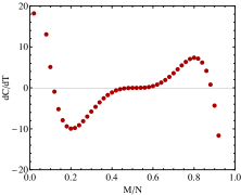
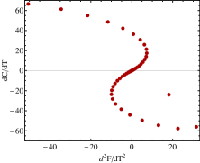
(a)  (b)

Figure 9: (a): $\mathrm{d}C/\mathrm{d}T$ versus $M/N$ for $N=50$. (b): $\mathrm{d}C/\mathrm{d}T$ versus $\mathrm{d}^{2}F/\mathrm{d}T^{2}$ for $N=50$. We note the stability region covers the second and third quadrant.

VI Possible generalizations beyond two-level systems

For tackling more realistic scenarios, the formalism presented above needs generalization. Now, in order to generalize the LMC measure proposed here to more realistic scenarios one must require that they exhibit quantifiable features. This is indeed possible in the cases of collective phenomena which emerge from real-world complex systems like traffic congestion, financial market crashes, wars, cancer, epidemics, etc. (see Ref. three ). If one has access to a measure $I$ that quantifies our ignorance with respect to some relevant aspects of the phenomena under scrutiny jaynes , then one can also assess its maximum possible possible value $I_{max}$ and construct a suitable LMC-like statistical complexity of the general form:

$$C_{I}=(1-I/I_{max})I,$$ (29)

a suitable generalization of (11). The foremost ignorance measure is Shannon’s one $H$ jaynes , so that

$$C_{Shannon}=(1-H/H_{max})H,$$ (30)

that does involve probabilities. However, these probabilities need not be the ones associated to Gibbs-ensembles. An example are the surrogate probabilities (12) above. This might be feasible for some of the complex scenarios envisaged in Ref. three and could then generate future research.

VII Conclusions

Most collective phenomena emerging from actual complex systems, like traffic jams, financial market moves, different types of conflicts etc., do not involve $10^{24}$ objects or agents but rather thousands, so that canonical ensemble considerations should better be replaced by micro-canonical ones, that do not involve probabilities. The successful complexity quantifier called statistical complexity assumes an underlying probability distribution, so that for using it in the above indicated scenarios it has to be adapted to a framework without probabilities. This is what we have done here for one of the simplest conceivable physical system: the two levels model.

Form another angle, note that binary decision problems represent a common scenario that yields a paramount example of real-world complexity three , providing researchers with a challenging problem which has, as far as we know, no exact mathematical theory to accompany it three . In this work a modest first step towards it has been taken, by expressing a binary decision in terms of occupying (or not) one of our two levels and $N$ particles, $M$ of which occupy the highest-lying one. We studied the set of the concomitant two-level configurations of $N-$particles and constructed statistical quantifiers for it like disequilibrium $D$ and statistical complexity $C$, without appeal to the notion of probability.

Our two-level configurations have fixed $E$ and $N$. Our focus was the collective of the $N,\,M$-configurations, each with different but fixed energy, particle-number, entropy, and temperature. We have described the properties of the collective, in particular, the values for $D$ and $C$. We have shown that $D$ is an order parameter and thus a thermodynamic variable. Accordingly, LMC’s statistical complexity became the product of two thermodynamic variables, something that, we believe, had not been remarked before.

Since $-d^{2}F/dT^{2}=C_{h}/T$, we were able to show that the $M/N-$location of the complexity maxima coincides with that of the $C_{h}$ ones, we conclude that the states of maximum complexity are the most stable ones, a very nice feature. We have seen that, for not too large $N-$values, configurations exist that are simultaneously complex and stable, which is remarkable given the system’s extreme simplicity. If one deals with a set of $N$ micro-canonical configurations labelled by an integer $M$, as here, each of them endowed with its own temperature $T_{M}$, one can successfully treat the set withe the surrogate probability distribution $P_{B}$ of Eq. (12).

We hope that our present close look to the inner workings of complexity in a simple environment will contribute to the elucidation of this notion and may stimulate other researchers to further delve on related issues.

References

- (1) R. López-Ruiz, H.L. Mancini, X. Calbet, Phys. Lett. A 209 (1995) 321.
- (2) R. López-Ruiz, International Journal of Bifurcation and Chaos 11 (2001) 2669.
- (3) M.T. Martin, A. Plastino, O.A. Rosso, Phys. Lett. A 311 (2003) 126.
- (4) L. Rudnicki, I.V. Toranzo, P. Sánchez-Moreno, J.S. Dehesa, Phys. Lett. A 380 (2016) 377.
- (5) R. López-Ruiz, H. Mancini, X. Calbet, A Statistical Measure of Complexity in Concepts and recent advances in generalized information measures and statistics, A. Kowalski, R. Rossignoli, E. M. C. Curado (Eds.), Bentham Science Books, pp. 147-168, New York, 2013.
- (6) K.D. Sen (Editor), Statistical Complexity, Applications in electronic structure, Springer, Berlin, 2011.
- (7) M. Mitchell, Complexity: A guided tour, Oxford University Press, Oxford, England, 2009.
- (8) M.T. Martin, A. Plastino, O.A. Rosso, Physica A 369 (2006) 439.
- (9) F. Pennnini, A. Plastino, Phys. Lett. A 381 (2017) 212.
- (10) N. F. Johnson, Two’s Company, Three is Complexity (Oneworld Publications, Oxford, England, 2007).
- (11) R. Lopez-Ruiz, Int. J. of Bifurc. and Chaos, . 11 (2001) 2669.
- (12) E.N. Miranda and Dalía S. Bertoldi. Thermostatistics of small systems: exact results in the microcanonical formalism. Eur. J. Phys. 34 (2013) 1075.
- (13) J. Kelly, Ensembles from Statistical Physics using Mathematica copyright James J. Kelly, 1996.
- (14) C. Kittel, Elementary statistical physics (John Wiley, NY, 19589.
- (15) N. F. Ramsey, Phys. Rev. 103 (1956) 20.
- (16) O. G. Jepps, G. Ayton, D. J. Evans, arXiv: cond-mat/9906423.
- (17) K. Huang, Statistical Mechanics (2 ed., Wiley, United States, 1987).
- (18) D. L. Stein, C. M. Newman, Spin glasses and complexity (Princeton University Press, Princeton, NJ, 2013).
- (19) H. B. Callen, Thermodynamics (John Wiley, NY, 1960).
- (20) D. Lynden-Bell, R. M. Lynden-Bell, Mon. Not. R. Astron. Soc. 181 (1977) 405.
- (21) E. A. Desloge, Thermal physics (Holt, Rinehart and Winston, NY, 1968).
- (22) P. W. Anderson, Science, 177 (1972) 393.
- (23) E.T. Jaynes, Phys. Rev. 106 (1957) 620; 118 (1961) 171; Papers on probability, statistics and statistical physics, edited by R. D. Rosenkrantz, Reidel, Dordrecht, Holland, 1983; L. Brillouin, Science and Information Theory, Academic Press, New York (1956); WT Grandy, Jr., and PW Milonni, Physics and probability: Essays in honor of E.T. Jaynes, Cambridge University Press, Cambridge, England, 1993.