Comparative study of finite element methods using the Time-Accuracy-Size (TAS) spectrum analysis

Abstract.

We present a performance analysis appropriate for comparing algorithms using different numerical discretizations. By taking into account the total time-to-solution, numerical accuracy with respect to an error norm, and the computation rate, a cost-benefit analysis can be performed to determine which algorithm and discretization are particularly suited for an application. This work extends the performance spectrum model in [16] for interpretation of hardware and algorithmic tradeoffs in numerical PDE simulation. As a proof-of-concept, popular finite element software packages are used to illustrate this analysis for Poisson’s equation.

1. Introduction

Computational scientists help bridge the gap between theory and application by translating mathematical techniques into robust software. One of the most popular approaches undertaken is the development of sophisticated finite element packages like FEniCS/Dolfin [30, 4], deal.II [9, 3], Firedrake [35], LibMesh [25], and MOOSE [21] which provide application scientists the necessary scientific tools to quickly address their specific needs. Alternatively, stand alone finite element computational frameworks built on top of parallel linear algebra libraries like PETSc [7, 8] may need to be developed to address specific technical problems such as enforcing maximum principles in subsurface flow and transport modeling [14, 15, 31] or modeling atmospheric and other geophysical phenomena [13, 32], all of which could require field-scale or even global-scale resolutions. As scientific problems grow increasingly complex, the software and algorithms used must be fast, scalable, and efficient across a wide range of hardware architectures and scientific applications, and new algorithms and numerical discretizations may need to be introduced. The ever increasing capacity and sophistication of processors, memory systems, and interconnects bring into question not only the performance of these new techniques, but their feasibility for large-scale problems. Specifically, how scalable is the software in both the algorithmic and parallel sense? Difficult problems require highly accurate numerical solutions, so it is desirable to take into consideration the solution accuracy along with both hardware utilization and algorithmic scalability. This paper is concerned with benchmarking the performance of various scientific software using analytic techniques.

1.1. Overview of scaling analyses

The most basic parallel scaling analysis, known as strong-scaling, looks at the marginal efficiency of each additional processor working on a given problem  [5, 18, 26]. A series of experiments is run using a fixed problem size but varying the number of processors used. It is typical to plot the number of processors $P$ against the speedup, defined as the time on one processor divided by the time on $P$ processors. Perfect speedup would result in a curve of unit positive slope. Because application scientists often have reason to solve a problem at a given resolution and spatial extent, strong-scaling is often of most interest: They may want to solve their problems in as little wall-clock time as possible, or, when running on shared resources, to complete a set of simulations in reasonable time without using too many CPU hours of their allocation (running in a strong-scaling “sweet spot” for their problem and machine). A simple strong-scaling analysis may, however, make it difficult to disentangle sources of inefficiency (serial sections, communication, latency, algorithmic problems, etc.).

In some cases, application scientists may be interested in exploring a problem at a range of resolutions or spatial extents. This leads naturally to weak-scaling  [22, 18, 26] scenarios: Instead of fixing the global problem size, they fix the portion of the problem on each processor and scale the entire problem size linearly with the number of processors. It is typical to plot the number of processors $P$ against the efficiency, defined as the time on one processor over the time on $P$ processors. Perfect efficiency would result in a flat curve at unity. This analysis shows the marginal efficiency of adding another subproblem, rather than just a processor, and separates communication overhead and algorithmic inefficiency from the problem of serial sections.

It is difficult to see, from either strong- or weak-scaling diagrams, how a given machine or algorithm will handle a variety of workloads. For example, is there is a minimum solution time where solver operations are swamped by latency? Is there a problem size where algorithmic pieces with suboptimal scaling start to dominate? We can examine these questions by running a series of problem sizes at fixed parallelism, called static-scaling [12, 16]. It is typical to plot the computation rate, in number of degrees-of-freedom (DoF) per time, against the time. Perfect scaling would result in a flat curve. Tailing off at small times is generally due to latency effects, and the curve will terminate at the smallest turnaround time for the machine. Decay at large times indicates suboptimal algorithmic performance or suboptimal memory access patterns and cache misses for larger problems. Thus we can see both strong- and weak-scaling effects on the same graph. It is also harder to game the result, since runtime is reported directly and extra work is directly visible. Static-scaling is a useful analytic technique for understanding the performance and scalability of PDE solvers across different hardware architectures and software implementations.

From the standpoint of scientific computing, a significant drawback of all of the above types of analyses is that they treat all computation equally and do not consider the theoretical convergence rate of the particular numerical discretization. The floating-point operations (FLOPs) done in the service of a quadratically convergent method, for instance, should be considered more valuable than those done for a linear method if both are in the basin of convergence. These analyses do not depend at all on numerical accuracy so the actual convergence behavior is typically measured empirically using the Method of Manufactured Solutions (MMS). If all equations are created equal, say for methods with roughly similar convergence behavior, then static-scaling is viable. However, it is insufficient when comparing methods with very different approximation properties. Any comparative study between different finite element methods or numerical discretization should factor accuracy into the scaling analyses.

1.2. Main contribution

The aim of this paper is to present an alternative performance spectrum model which takes into account time-to-solution, accuracy of the numerical solution, and size of the problem hence the Time-Accuracy-Size (TAS) spectrum analysis. These are the three metrics of most importance when a comparative study involving different finite element or any numerical methods is needed. Not every DoF has an equal contribution to the discretization’s level of accuracy, so the DoF per time metric alone would be neither a fair nor accurate way of assessing the quality of a particular software’s implementation of the finite element method. An outline of the salient features of this paper are listed below:

• We provide a modification to the static-scaling analysis incorporating numerical accuracy.

• We present the TAS spectrum and discuss how to analyze its diagrams.

• Popular software packages, such as FEniCS/Dolfin, deal.II, Firedrake, and PETSc, are compared using the Poisson problem.

• Different single-field finite element discretizations, such as the Galerkin and Discontinuous Galerkin methods, are also compared.

• The analysis is extended to larger-scale computations, i.e. over 1K MPI processes.

The rest of the paper is organized as follows. In Section 2, we present the framework of the Time-Accuracy-Size (TAS) spectrum model and outline how to interpret the diagrams. In Section 3, we provide a theoretical derivation of the TAS spectrum and provide example convergence plots one may expect to see. In Section 4, we describe in detail how the finite element experiments are setup. In Section 5, we demonstrate various ways the TAS spectrum is useful by running various test cases. Conclusions and possible extensions of this work are outlined in Section 6.

2. TAS Spectrum

In order to incorporate accuracy into our performance analysis, we must first have an idea of convergence, or alternatively the numerical accuracy of a solution. In this paper, we will measure solution accuracy using the $L_{2}$ norm of the error $err$,

$$err=\left\lVert u_{h}-u\right\rVert_{L_{2}},$$ (1)

where $u_{h}$ is the finite element solution, $u$ is the exact solution, and $h$ is some measure of our resolution such as the longest edge in any mesh element. Convergence means that our error shrinks as we increase our resolution, so that $\lim_{h\to 0}err=0$. In fact, we expect most discretization methods to have a relation of the form

$$err\leq Ch^{\alpha},$$ (2)

where $C$ is some constant and $\alpha$ is called the convergence rate of the method. This relation can be verified by plotting the logarithm of the resolution $h$ against the negative logarithm of the error $err$, which we call the digits of accuracy (DoA),

$$\mathrm{DoA}=-\log_{10}err.$$ (3)

This should produce a line with slope $-\alpha$, and is typically called a mesh convergence diagram [11, 26]. If we use the number of unknowns $N$ (or DoF) instead of the resolution $h$, the slope of the line will be modified. For most schemes $N=Dh^{-d}$, where $d$ is the spatial dimension and $D$ is a constant, so that the slope would become $\alpha/d$. In our development, we will use this form of convergence diagram and call $\log_{10}N$ the digits of size (DoS). Much as weak-scaling explains the behavior of algorithm on a range of problem sizes, the mesh-convergence diagram explains the behavior of a discretization.

In order to incorporate accuracy information, we will imitate the static-scaling analysis by examining the rate of accuracy production. We will introduce a measure called efficacy, defined to be error multiplied by time. Smaller efficacy is desirable, as this means either smaller error or smaller time. We introduce the digits of efficacy (DoE) as the logarithm of error multiplied by time. As shown in Section 3, this rate has a linear dependence on problem size, and slope $d-\alpha$. Our accuracy scaling analysis plots digits of efficacy against time. This analysis will be able to compare not only different parallel algorithms and algebraic solvers, but also discretizations, as demonstrated in Section 5.

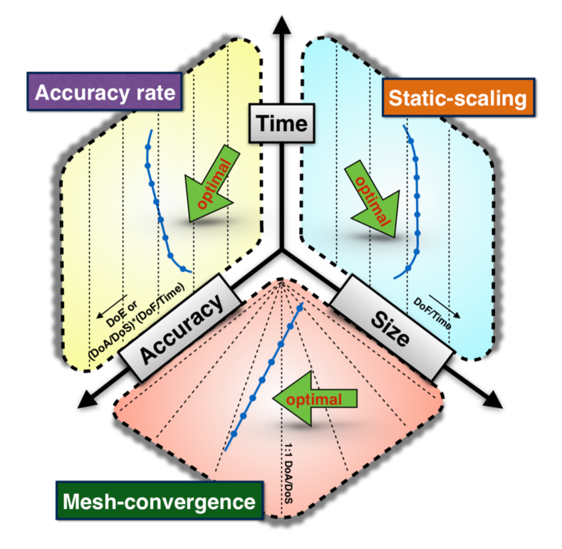
(a)

Figure 1. Pictorial description of the Time-Accuracy-Size (TAS) spectrum.

We now present the Time-Accuracy-Size (TAS) spectrum. In Figure 1, we show the relation of our new efficacy analysis to the existing mesh convergence and static scaling plots. As outlined in [16], static-scaling measures the degrees of freedom solved per second for a given parallelism. That is,

$$\mbox{Static-scaling}\qquad\mathrm{measures}\qquad\left(\frac{\mathrm{size}/\mathrm{time}}{\mathrm{time}}\right)$$ (4)

We assume that the problems are of linear complexity, i.e. the time is in $\mathcal{O}(N)$, so optimal scaling is indicated by a horizontal line as the problem size is increased. A higher computation rate indicates that the algorithm matches the hardware well, but tells us little about how accurate the solution is. Measures of the accuracy as a function of problem size, however, are basic to numerical analysis, and usually referred to as mesh convergence,

$$\mbox{Mesh-convergence}\qquad\mathrm{measures}\qquad\left(\frac{1/\mathrm{error}}{\mathrm{size}}\right)$$ (5)

where we use the inverse of error since we usually measure the negative logarithm of the error. Multiplying equations (4) and (5) together, we arrive at rate for accuracy production,

$$\mbox{Accuracy rate}\qquad\mathrm{measures}\qquad\left(\frac{1/\mathrm{error}}{\mathrm{size}}\right)\times\left(\frac{\mathrm{size}/\mathrm{time}}{\mathrm{time}}\right)=\frac{1/(\mathrm{error}\times\mathrm{time})}{\mathrm{time}},$$ (6)

which is exactly our efficacy measure. An alternate derivation would be to scale the DoF count used in the typical static-scaling analysis by the mesh convergence ratio, which we call true static-scaling. This produces the same measure, but slightly different scaling when logarithms are applied. Looking at equations (4), (5), and (6) give us the TAS spectrum, as visually depicted in Figure 1. This figure illustrates how the new efficacy analysis can be applied to the existing mesh convergence and static scaling plots.

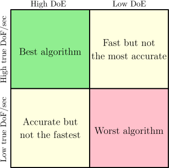
(a)

Figure 2. Interpretation of both the DoE and true DoF per second metrics of a particular algorithm. DoE is often an indicator of how accurate an algorithm is for a given amount of time, whereas true DoF per time is often an indicator of how fast an algorithm processes each DoF when each DoF is scaled by how much accuracy it contributes.

2.1. Interpreting the TAS spectrum

The complete TAS spectrum could potentially have three or four different diagrams that provide a wealth of performance information. We now show the recommended order of interpretation of these diagrams as well as provide some guidelines on how to synthesize the data into an understandable framework.

1. Mesh convergence: This diagram not only shows whether the actual $L_{2}$ convergence matches the predicted $\alpha$, but how much accuracy is attained for a given size. Any tailing off that occurs in the line plots could potentially be an issue of solver tolerance or implementation errors. Such tail-offs will drastically affect both accuracy rate diagrams, so this diagram could be an early warning sign for unexpected behavior in those plots. Furthermore, the mesh convergence ratio (i.e., the DoA over DoS) can also be an early predictor as to which discretizations or implementations will have better accuracy rates.

2. Static-scaling: This particular scaling analysis is particularly useful for examining both strong-scaling and weak-scaling limits of parallel finite element simulations across various hardware architectures and software/solver implementations. Optimal scaling would produce a horizontal line or a “sweet spot” assuming that the algorithm is of $\mathcal{O}(N)$ complexity. Any tailing off in these static-scaling plots will have a direct affect on the accuracy rate plots.

3. DoE: This metric gives the simplest interpretation of numerical accuracy and computational cost. A high DoE is most desired, and if straight lines are observed in both the mesh convergence and static-scaling diagrams, the lines in this diagram should exhibit some predicted slope which will be discussed in the next section. Note that the size of the problem is not explicitly taken into account in these diagrams; these diagrams simply provide an easy visual on the ordering of the software implementation or finite element discretization.

4. True static-scaling: Optionally, the ordering shown in the DoE diagrams can be further verified through the true static-scaling plots. The information provided by this analysis simply tells us how fast the algorithm is being computed assuming that all DoF are given equal weighting. Figure 2 provides a simple guideline on how to simultaneously interpret both the DoE and true static-scaling diagrams. Note that the true static-scaling diagrams will not always produce a horizontal line, as the DoF is now scaled by the DoA over DoS ratio.

3. Theoretical Analysis

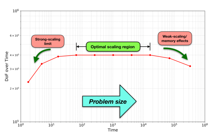
(a)

Figure 3. Example static-scaling diagram and a description of the behavioral characteristics. This diagram is able to characterize both strong-scaling and weak-scaling effects across a variety of problem sizes.

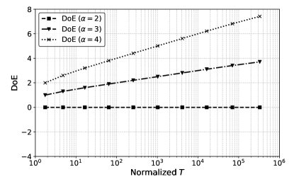
(a) $d=2$

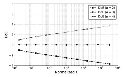
(b) $d=3$

Figure 4. Example DoE diagrams for 2D and 3D problems assuming $C=10$, $W=0.1$ and that $h$-sizes range from 1/10 to 1/5120. Both $\alpha$ and $d$ have a drastic effect on the slope of these lines.

Unlike the mesh convergence and static-scaling analyses, the accuracy rate diagrams, which consist of the DoE and the true DoF per time metrics, measure the accuracy achieved by a particular method in a given amount of time. In this Section, we will discuss the theoretical underpinning of these two diagrams and examine the behavior of the line plots. The DoE is written as:

$$\mathrm{DoE}\ =-\log_{10}(err\times T).$$ (7)

Recall that $err\leq Ch^{\alpha}$ is the $L_{2}$ norm of the error with a theoretical convergence rate $\alpha$, which can be obtained directly using MMS, and $T$ is the time:

$$T=Wh^{-d},$$ (8)

where $d$ is the spatial dimension, $h$ denotes the representative element length, and $C$ and $W$ are constants. Then for a given run, the digits of efficacy would be given by

$$\mathrm{DoE} =-\log_{10}\left(Ch^{\alpha}Wh^{-d}\right)$$ (9)

$$=-\log_{10}\left(CWh^{\alpha-d}\right)$$ (10)

$$=(d-\alpha)\log_{10}(h)-\log_{10}(CW).$$ (11)

Since $C$ and $W$ are constants, the slopes of the DoE lines are only affected by $\alpha$ and $d$. However, because of strong-scaling and weak-scaling limits, it is possible that the time $T$ may not always be of linear complexity thus the slope may not actually be $d-\alpha$. Let us consider a simple static-scaling example shown in Figure 3. It can be seen here that the DoF per time (or $N/T$) ratios indicate at what points both strong-scaling and weak-scaling/memory effects start to dominate for a given MPI parallelism. If $C=10$, $W=0.1$, and $h$-sizes ranging from 1/10 to 1/5120, we can see from Figure 4 what type of slopes we could expect to see in the DoE diagrams assuming the same $T$ from Figure 3. It can be seen that methods with higher order rates of convergence are preferable as $h$ is refined. For this particular example’s chosen parameters, it can also be seen that the strong-scaling effects skew a few of the data points at the beginning but the weak-scaling effects are nearly unseen. Such effects may not aways be negligible in these DoE diagrams but could be carefully noted from static-scaling.

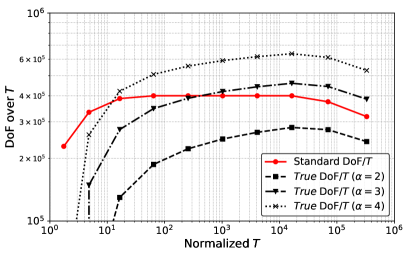
(a) $h$-size range: 10^-1 to 10^-3

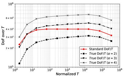
(b) $h$-size range: 10^-2 to 10^-4

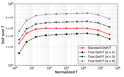
(c) $h$-size range: 10^-3 to 10^-5

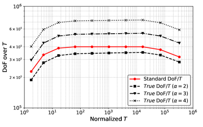
(d) $h$-size range: 10^-5 to 10^-7

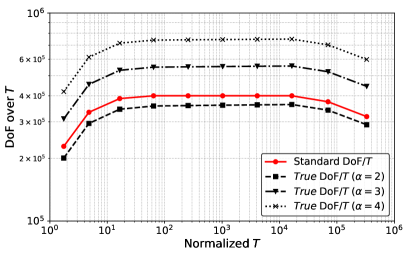
(e) $h$-size range: 10^-7 to 10^-9

(f) $h$-size range: 10^-10 to 10^-12

Figure 5. True DoF per time rates in comparison to the original DoF per time rate for various $h$-sizes and $\alpha$. Let $d=2$, $C=10$, $D=4$, and the optimal DoF/$T=4\times 10^{5}$.

In true static-scaling, the DoF per time metric needs to be scaled by the mesh convergence ratio DoA/DoS. Before we get into the analysis of this scaling plot, we list a few key assumptions that must be made in order for this to work:

1. Problem size DoF or $N=Dh^{-d}$ where $D$ is a constant.

2. All computations are of linear complexity i.e., $\mathcal{O}(N)$.

3. Any tailing off from $\mathcal{O}(N)$ occurs due to hardware related issues like latency from strong-scaling effects, memory bandwidth contention, or cache misses.

4. The problem size $N$ or DoF must be greater than 1.

5. $L_{2}$ error norm $err<1.0$.

Any violations to the last two assumptions would require that a different logarithm rule be used or for the numbers to be scaled so that neither DoA nor DoS are zero. The behavior of the true static-scaling line plot is given by:

$$\left(\frac{\mathrm{DoA}}{\mathrm{DoS}}\right)\times\left(\frac{N}{T}\right) =\left(\frac{-\log_{10}(Ch^{\alpha})}{\log_{10}(Dh^{-d})}\right)\times\left(\frac{Dh^{-d}}{Wh^{-d}}\right)$$ (12)

$$=\frac{-\log_{10}(C)-\log_{10}(h^{\alpha})}{\log_{10}(D)+\log_{10}(h^{-d})}\times\left(\frac{D}{W}\right)$$ (13)

$$=\frac{-\alpha\log_{10}(h)-\log_{10}(C)}{-d\log_{10}(h)+\log_{10}(D)}\times\left(\frac{D}{W}\right).$$ (14)

The variables $\alpha$, $d$, $C$, and $D$ will significantly impact the qualitative behavior of the true static-scaling diagrams. As $h$ approaches zero, the $N/T$ ratio will slowly asymptote to a new $N/T$ ratio scaled by the factor $\alpha/d$. Consider the following true-static scaling diagrams in Figure 5 when $d=2$, $C=10$, $D=4$, and a variety of $h$-sizes are examined. It can be seen here that for larger $h$-sizes or coarser meshes, the DoF/$T$ lines are drastically skewed, and the optimal scaling regions are no longer horizontal. The relative ordering of the line plots in both accuracy rate diagrams depend significantly on the constants $C$, $D$, and $W$.

4. Experimental Setup

In this paper, we only consider the Poisson equation,

$$-\nabla^{2}u =f, u \in\Omega$$ (15)

$$u =u_{0}, u \in\Gamma_{D}$$ (16)

where $\Omega$ denotes the computational domain in $\mathbb{R}^{d}$, $\Gamma_{D}$ denotes its boundary, $u$ is the scalar solution field, and $u_{0}$ are the prescribed Dirichlet boundary values.

The finite element discretizations considered are the Continuous Galerkin (CG) and Discontinuous Galerkin (DG) methods. Various levels of both $h$- and $p$-refinement for the CG and DG methods are considered across different software implementations. We do not consider other viable approaches such as the Hybridizable Discontinuous Galerkin (HDG) method [24, 19] or mixed formulations [36, 17] but these will be addressed in future work. To this end, let us define $E$ as an element belonging to a mesh $\mathcal{E}(\Omega)$. The relevant finite-dimensional function space for simplices is

$$\mathcal{U}_{h} :=\left\{u_{h}\in L^{2}(\Omega):\;u_{h}\big{|}_{E}\in\mathcal{P}_{p}(E)\quad\forall\ E\in\mathcal{E}(\Omega)\right\},$$ (17)

and for tensor product cells is

$$\mathcal{U}_{h} :=\left\{u_{h}\in L^{2}(\Omega):\;u_{h}\big{|}_{E}\in\mathcal{Q}_{p}(E)\quad\forall\ E\in\mathcal{E}(\Omega)\right\}.$$ (18)

Here $\mathcal{P}_{p}(E)$ denotes the space of polynomials in $d$ variables of degree less than or equal to $p$ over the element $E$, and $\mathcal{Q}_{p}(E)$ is the space of $d$-dimensional tensor products of polynomials of degree less than or equal to $p$. The general form of the weak formulation for equation (15) can be written as follows: Find $u_{h}\in\mathcal{U}_{h}$ such that

$$\mathcal{B}\left(v_{h};u_{h}\right)=\mathcal{L}\left(v_{h}\right)\quad\forall\ v_{h}\in\mathcal{U}_{h}$$ (19)

where $\mathcal{B}$ and $\mathcal{L}$ denote the bilinear and linear forms, respectively.

4.1. Finite element discretizations

For the CG discretization, the solution $u_{h}$ is continuous at element boundaries, so that $\mathcal{U}_{h}$ is actually a subspace of $H^{1}$, and the test functions satisfy $v_{h}=u_{0}$ on $\Gamma_{D}$. To present the DG formulation employed in the paper, we introduce some notation. The boundary of a cell $E_{i}$ is denoted by $\partial E_{i}$. The interior face between $E_{i}$ and $E_{j}$ is denoted by $\Gamma_{ij}$. That is,

$$\Gamma_{ij}=\partial E_{i}\cap\partial E_{j}$$ (20)

The set of all points on the interior faces is denoted by $\Gamma_{\mathrm{int}}$. Mathematically,

$$\Gamma_{\mathrm{int}}=\bigcup_{i,j}^{\mathcal{E}(\Omega)}\Gamma_{ij}$$ (21)

For an interior face, we denote the subdomains shared by this face by $E^{+}$ and $E^{-}$. The outward normals on this face for these cells are, respectively, denoted by $\widehat{\mathbf{n}}^{+}$ and $\widehat{\mathbf{n}}^{-}$. Employing Brezzi’s notation [6], the average and jump operators on an interior face are defined as follows

$$\big{\{}c\big{\}}:=\frac{c^{+}+c^{-}}{2}\quad\mathrm{and}\quad\big{[}\!\big{[}c\big{]}\!\big{]}:=c^{+}\widehat{\mathbf{n}}^{+}+c^{-}\widehat{\mathbf{n}}^{-}$$ (22)

where

$$c^{+}=c|_{\partial E^{+}}\quad\mathrm{and}\quad c^{-}=c|_{\partial E^{-}}$$ (23)

Let $\Gamma_{D}$ denote the set of all boundary faces. For a face $e\in\Gamma_{D}$, we then define $\{c\}=c|_{e}$, and $[\![c]\!]=c|_{e}\widehat{\mathbf{n}}_{e}.$ One of the most popular DG formulations is the Symmetric Interior Penalty method, which for equation (19) is written

$$\mathcal{B}(v_{h};u_{h}) :=\sum_{E\in\mathcal{E}(\Omega)}\int_{E}\nabla v_{h}\cdot\nabla u_{h}-\sum_{e\in\Gamma_{\mathrm{int}}\cup\Gamma_{D}}\int_{e}\{v_{h}\}\cdot\big{[}\!\big{[}u_{h}\big{]}\!\big{]}-\sum_{e\in\Gamma_{\mathrm{int}}\cup\Gamma_{D}}\int_{e}\{u_{h}\}\cdot\big{[}\!\big{[}v_{h}\big{]}\!\big{]}$$

$$+\sigma\sum_{e\in\Gamma_{\mathrm{int}}}\int_{e}\frac{|e|}{|E|}\big{[}\!\big{[}v_{h}\big{]}\!\big{]}\cdot\big{[}\!\big{[}u_{h}\big{]}\!\big{]}+\gamma\sum_{e\in\Gamma_{D}}\int_{e}\frac{|e|}{|E|}v_{h}u_{h}$$ (24)

$$\mathcal{L}(v_{h}) :=\sum_{E\in\mathcal{E}(\Omega)}\int_{E}v_{h}f-\sum_{e\in\Gamma_{\mathrm{D}}}\int_{e}u_{0}\nabla v_{h}\cdot\widehat{\mathbf{n}}_{e}+\gamma\sum_{e\in\Gamma_{\mathrm{D}}}\int_{e}\frac{|e|}{|E|}v_{h}u_{0}$$ (25)

where $\widehat{\mathbf{n}}_{e}$ denotes the outward normal on an exterior face, $|e|$ is the measure of a face in the given triangulation, $|E|$ is the measure of a cell in the given triangulation, and the penalty terms $\alpha$ and $\gamma$ are written as:

$$\sigma =\frac{(p+1)(p+d)}{2d}$$ (26)

$$\gamma =2\alpha$$ (27)

as described in  [39].

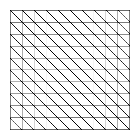
(a)

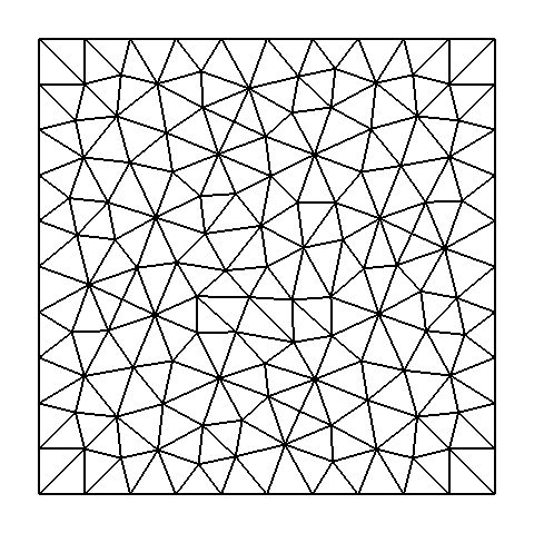
(b)

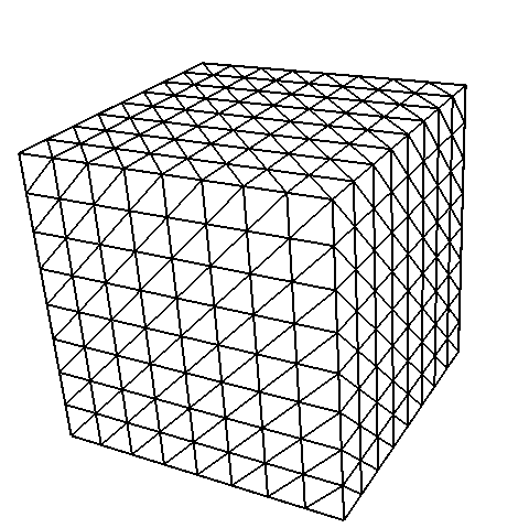
(c)

(d)

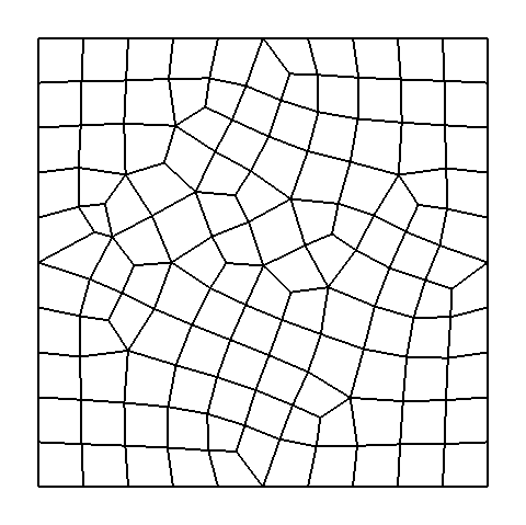
(e)

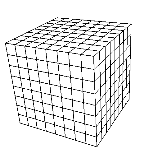
(f)

Figure 6. The structured and unstructured grids considered in this paper.

4.2. Software and solver implementation

In the next section, four different test problems are considered to demonstrate the unique capabilities of the TAS spectrum analysis. For the first three problems, the following sophisticated finite element software packages are examined: the C++ implementation of the FEniCS/Dolfin Project (Docker tag: 2017.1.0.r1), the the Python implementation of the Firedrake Project (SHA1: v0.13.0-1773-gc4b38f13), and the C++ implementation of the deal.II library (Docker tag: v8.5.1-gcc-mpi-fulldepscandi-debugrelease). All three packages use various versions of PETSc for the solution of linear and nonlinear systems. The last problem utilizes the development version of PETSc (SHA1: v3.8.3-1636-gbcc3281268) and its native finite element framework. The FEniCS/Dolfin/Firedrake software calculate the $L_{2}$ error norms by projecting the analytical solution $u$ onto a function space 3 degrees order higher than the finite element solution $u_{h}$, whereas both deal.II and PETSc do the integral directly and use the same function space for both $u$ and $u_{h}$.

The test problems will be tested on the various meshes depicted in Figure 6. The FEniCS/Dolfin and deal.II libraries use custom meshing, while Firedrake uses PETSc to manage unstructured meshes  [27, 29, 28], and the hexahedral meshes are generated using the algorithms described in [10, 33, 23]. All timings will simply measure the finite element assembly and solve steps but not the mesh generation or any other preprocessing steps.

The first three test problems presented in this paper will be solved using the conjugate gradient method with HYPRE’s algebraic multigrid solver, BoomerAMG [20], and have a relative convergence criterion of $10^{-7}$. The last problem will also consider two other multigrid solvers—the PETSc-native GAMG preconditioner [1, 2] and Trilinos’ Multi-Level (ML) solver [37]—but have a relative convergence criterion of $10^{-9}$.

The first three tests are conducted on a single 3.5 GHz Quad-core Intel Core i5-7600 processor with 64 GB of 2400 MHz DDR4 memory. The two (2D) problems are run in serial whereas the third (3D) problem is run across 4 MPI processes. The last problem is conducted on the Cori Cray XC40 system at the National Energy Research Scientific Computing Center (NERSC), and utilizes 32 Intel Xeon E5-2698v3 (“Haswell”) nodes for a total of 1024 MPI processes.

5. Computational Results

5.1. Test #1: Software implementation and mesh types

Table 1. Comparison of CG1 across packages

DoF	DoS	FEniCS - triangles		Firedrake - triangles		Firedrake - quads		deal.II - quads
		DoA	DoA/DoS	DoA	DoA/DoS	DoA	DoA/DoS	DoA	DoA/DoS
Structured
121	2.08	1.11	0.52	1.08	0.50	1.32	0.63	1.71	0.82
441	2.64	1.66	0.61	1.65	0.61	1.91	0.72	2.31	0.87
1681	3.23	2.25	0.68	2.24	0.68	2.50	0.78	2.92	0.90
6561	3.82	2.84	0.73	2.84	0.73	3.10	0.81	3.52	0.92
25921	4.41	3.41	0.77	3.44	0.77	3.71	0.84	4.12	0.93
103041	5.01	4.04	0.79	4.04	0.79	4.31	0.86	4.72	0.94
Unstructured
142	2.15	1.27	0.59	1.27	0.59	1.30	0.63	1.63	0.76
525	2.72	1.84	0.68	1.84	0.68	1.89	0.72	2.23	0.82
2017	3.30	2.44	0.74	2.44	0.74	2.49	0.77	2.83	0.86
7905	3.90	3.04	0.78	3.04	0.78	3.09	0.81	3.43	0.88
31297	4.50	3.64	0.81	3.64	0.81	3.69	0.84	4.03	0.90
124545	5.10	4.24	0.83	4.24	0.83	4.29	0.86	4.64	0.91

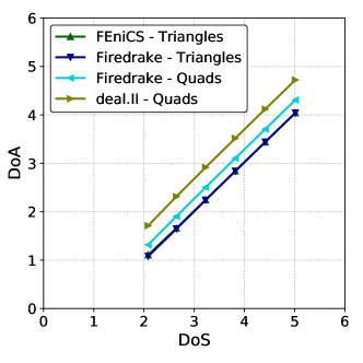
(a) Mesh convergence: Structured

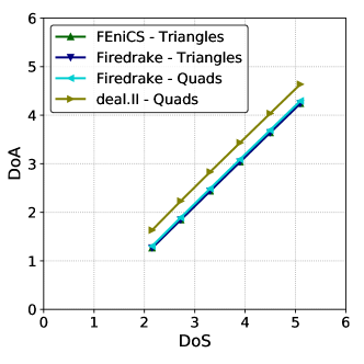
(b) Mesh convergence: Unstructured

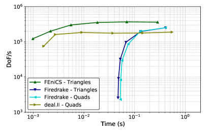
(c) Static-scaling: Structured

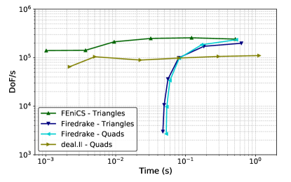
(d) Static-scaling: Unstructured

Figure 7. Test #1: Mesh convergence and static-scaling comparing various finite element software packages on structured and unstructured 2D grids.

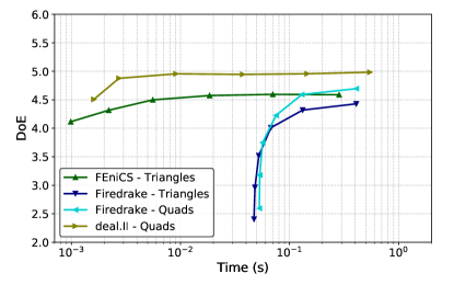
(a) DoE: Structured

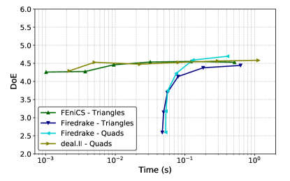
(b) DoE: Unstructured

(c) True static-scaling: Structured

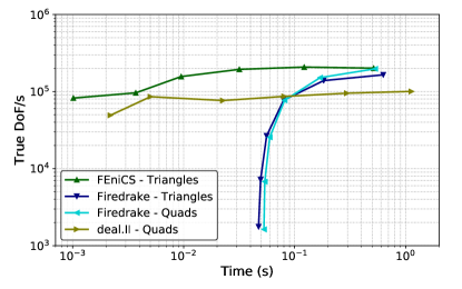
(d) True static-scaling: Unstructured

Figure 8. Test #1: Accuracy rates comparing various finite element software packages on structured and unstructured 2D grids.

First, we examine how the first-order CG discretization performs on both structured and unstructured grids as implemented in the three different software packages. Consider the following analytical solution on a unit square,

$$u(x,y)=\sin(2\pi x)\sin(2\pi y).$$ (28)

The 2D initial coarse grids shown in Figure 6 and are refined up to 5 times. Information concerning the DoS and DoA for these problems can be found in Table 1. It should be noted that while the Firedrake library is capable of handling both triangular and quadrilateral elements, the FEniCS and deal.II libraries are only capable of handling, respectively, triangular and quadrilateral elements.

Figure 7 contain the mesh convergence and static-scaling diagrams. From the mesh-convergence diagrams, we see that the unit slope matches our prediction $\frac{\alpha}{d}=1$ for a second order method in two dimensions. The static-scaling diagrams indicate that that FEniCS/Dolfin and Firedrake have very similar performances and outperform deal.II on large problems. However, as the problem size decreases (approaching the strong-scaling limit) the overhead in Firedrake becomes apparent. Note that deal.II and Firedrake’s quadrilateral meshes give slightly more accurate solutions so we now examine the two accuracy rate metrics in Figure 8. The DoE plots indicate that the quadrilateral meshes are in fact the more accurate methods, especially for the structured grids. The true static-scaling plots indicate that while the deal.II results may be the most accurate, they are not the fastest in terms of processing the DoFs. The TAS spectrum analysis suggests that quadrilateral meshes not only offer more accuracy but are also faster so long as the software is implemented efficiently.

5.2. Test #2: CG vs DG with same $h$-size

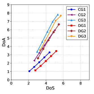
(a) Mesh- convergence: FEniCS

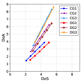
(b) Mesh-convergence: deal.II

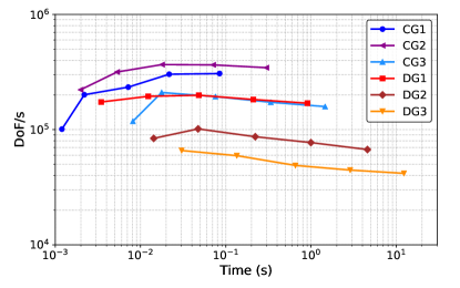
(c) Static-scaling: FEniCS

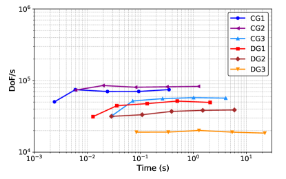
(d) Static-scaling: deal.II

Figure 9. Test #2: Mesh convergence and static-scaling on structured grids comparing 2D CG and DG when the $h$-size is the same.

Table 2. Comparison of 2D structured grid (same $h$) CG and DG in FEniCS

$h$-size	CG1			CG2			CG3
	DoA	DoS	DoA/DoS	DoA	DoS	DoA/DoS	DoA	DoS	DoA/DoS
1/10	1.04	2.08	0.50	2.31	2.64	0.88	3.37	2.98	1.13
1/20	1.55	2.64	0.59	3.23	3.23	1.00	4.56	3.57	1.28
1/40	2.11	3.23	0.65	4.15	3.82	1.09	5.76	4.17	1.38
1/80	2.70	3.82	0.71	5.06	4.41	1.15	6.96	4.76	1.46
1/160	3.30	4.41	0.75	5.96	5.01	1.19	7.82	5.36	1.45
$h$-size	DG1			DG2			DG3
	DoA	DoS	DoA/DoS	DoA	DoS	DoA/DoS	DoA	DoS	DoA/DoS
1/10	1.15	2.78	0.41	2.59	3.08	0.84	3.54	3.30	1.07
1/20	1.68	3.38	0.50	3.70	3.68	1.01	4.67	3.90	1.20
1/40	2.26	3.98	0.57	4.76	4.28	1.11	5.86	4.51	1.30
1/80	2.85	4.58	0.62	5.72	4.89	1.17	7.07	5.11	1.38
1/160	3.45	5.19	0.66	6.65	5.49	1.21	7.67	5.71	1.34

Table 3. Comparison of 2D structured grid (same $h$) CG and DG in deal.II

$h$-size	CG1			CG2			CG3
	DoA	DoS	DoA/DoS	DoA	DoS	DoA/DoS	DoA	DoS	DoA/DoS
1/10	1.45	2.08	0.70	2.65	2.64	1.00	3.50	2.98	1.17
1/20	2.05	2.64	0.88	3.53	3.23	1.10	4.71	3.57	1.32
1/40	2.65	3.23	0.82	4.43	3.82	1.16	5.91	4.17	1.42
1/80	3.26	3.82	0.85	5.33	4.41	1.21	7.12	4.76	1.49
1/160	3.86	4.41	0.87	6.24	5.01	1.24	8.32	5.36	1.55
$h$-size	DG1			DG2			DG3
	DoA	DoS	DoA/DoS	DoA	DoS	DoA/DoS	DoA	DoS	DoA/DoS
1/10	1.55	2.60	0.59	2.75	2.95	0.93	3.88	3.20	1.21
1/20	2.08	3.20	0.65	3.69	3.56	1.04	5.00	3.81	1.31
1/40	2.66	3.81	0.70	4.61	4.16	1.11	6.17	4.41	1.40
1/80	3.26	4.41	0.74	5.52	4.76	1.16	7.37	5.01	1.47
1/160	3.86	5.01	0.77	6.42	5.36	1.20	8.57	5.61	1.53

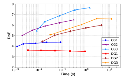
(a) DoE: FEniCS

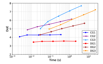
(b) DoE: deal.II

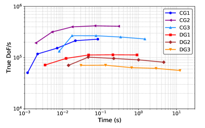
(c) True static-scaling: FEniCS

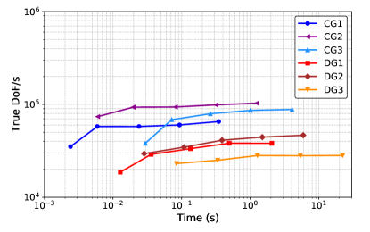
(d) True static-scaling: deal.II

Figure 10. Test #2: Accuracy rates on structured grids comparing 2D CG and DG when the $h$-size is the same.

Next, we examine the behavior of different finite element discretizations for a given refinement, or $h$ size. Three levels of $p$-refinement are considered on a unit square domain with the following analytical solution,

$$u(x,y)=\sin(2\pi x^{2})\sin(2\pi y^{2}).$$ (29)

We consider only the CG and SIP DG discretizations, with the value of the penalty chosen based on the formula derived in [39]. Both FEniCS/Dolfin and deal.II are used for this case, starting with the structured meshes on the left of Figure 6 as the initial meshes and using four levels of refinement. The DoS and DoA for the FEniCS/Dolfin and deal.II discretizations can be found in Tables 2 and 3, respectively. From the mesh-convergence diagrams in Figure 9, we see that second order methods have unit slope, the third order methods have slope $\frac{3}{2}$, and fourth order methods have slope 2, as predicted. It is interesting to note that FEniCS’s fourth order methods experience a dropoff in convergence when the DoA goes past 7.0, which arises due to the relative convergence criterion of 10^-7.

In the static-scaling diagrams in Figure 9, we see that the high order methods show greater fall off as problem size increases. Since the number of solver iterates remains roughly constant, this is due to AMG solver complexity rising at a slightly nonlinear rate. Moreover, the CG methods perform at a strictly higher rate than their DG counterparts, and within the CG and DG classes, lower order methods are operating faster than high order, with the exception of CG2. When we introduce the notion of accuracy into Figure 10, however, this traditional analysis is upended. Now, within CG or DG, each order produces accuracy faster than the order below as seen from the scaled error diagrams. From the true static-scaling diagrams, it can be seen that the CG methods are slightly more efficient. For example, DG3 may be one of the most accurate methods for smaller $h$-sizes but is clearly the slowest at processing its DoFs if all DoFs are given equal treatment.

5.3. Test #3: CG vs DG with same DoF count

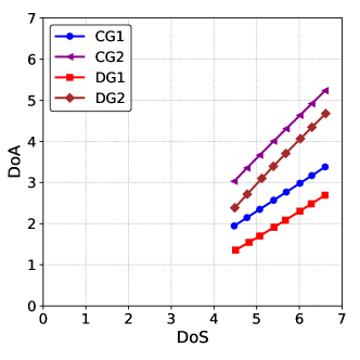
(a) Mesh-convergence: Tetrahedrons

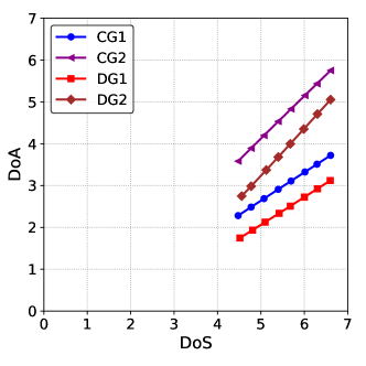
(b) Mesh-convergence: Hexahedrons

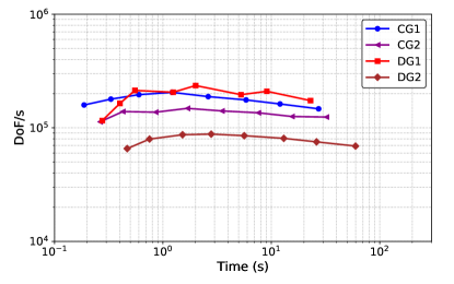
(c) Static-scaling: Tetrahedrons

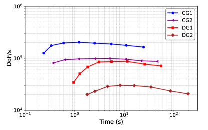
(d) Static-scaling: Hexahedrons

Figure 11. Test #3: Mesh convergence and static-scaling on structured grids comparing CG and DG when the DoF is the same.

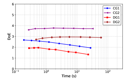
(a) DoE: Tetrahedrons

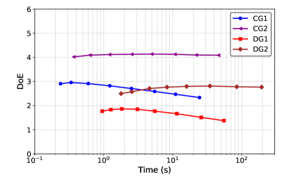
(b) DoE: Hexahedrons

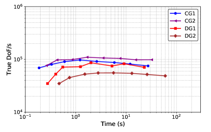
(c) True static-scaling: Tetrahedrons

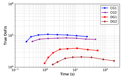
(d) True static-scaling: Hexahedrons

Figure 12. Test #3: Accuracy rates on structured grids comparing 3D CG and DG when the DoF the same.

It can be seen from the previous test that each discretization has a different DoF count for a given mesh, making it somewhat difficult to draw any comparisons. This can be especially true for 3D problems where the problem size proliferates even more for every step of mesh refinement. In this third test, each finite element discretization will have roughly the same DoF count by adjusting the $h$-size. Using Firedrake, the CG and DG discretizations with up to 2 different levels of $p$-refinement are considered for the following analytical solution on a unit cube,

$$u(x,y,z)=\sin(2\pi x)\sin(2\pi y)\sin(2\pi z).$$ (30)

Both tetrahedral and hexahedral elements from Figure 6 are used and Tables 4 and 5 depict the $h$-sizes needed in order for all the discretizations to have roughly the same DoS. From Figure 11, we see that second order methods have slope $\frac{2}{3}$, since now $d=3$, and the third order methods have unit slope, as predicted.

Table 4. Comparison of 3D structured grid with tetrahedron elements (same DoF) CG and DG in Firedrake

CG1				CG2
$h$-size	DoA	DoS	DoA/DoS	$h$-size	DoA	DoS	DoA/DoS
1/30	1.96	4.47	0.43	1/15	3.03	4.47	0.68
1/38	2.15	4.77	0.45	1/19	3.35	4.77	0.70
1/48	2.35	5.07	0.46	1/24	3.67	5.07	0.72
1/62	2.57	5.40	0.48	1/31	4.01	5.40	0.74
1/78	2.77	5.69	0.49	1/39	4.31	5.69	0.76
1/100	2.98	6.01	0.50	1/50	4.63	6.01	0.77
1/124	3.17	6.29	0.50	1/62	4.92	6.29	0.78
1/158	3.38	6.60	0.51	1/79	5.23	6.60	0.79
DG1				DG2
$h$-size	DoA	DoS	DoA/DoS	$h$-size	DoA	DoS	DoA/DoS
1/11	1.36	4.50	0.30	1/8	2.39	4.49	0.53
1/14	1.55	4.82	0.32	1/10	2.72	4.78	0.57
1/17	1.70	5.07	0.34	1/13	3.10	5.12	0.61
1/22	1.91	5.41	0.35	1/16	3.39	5.39	0.63
1/27	2.09	5.67	0.37	1/20	3.71	5.68	0.65
1/35	2.31	6.01	0.38	1/26	4.06	6.02	0.67
1/43	2.48	6.28	0.40	1/32	4.34	6.29	0.69
1/55	2.69	6.60	0.41	1/41	4.67	6.62	0.71

Table 5. Comparison of 3D structured grid with hexahedron elements (same DoF) CG and DG in Firedrake

CG1				CG2
$h$-size	DoA	DoS	DoA/DoS	$h$-size	DoA	DoS	DoA/DoS
1/30	2.28	4.47	0.51	1/15	3.58	4.47	0.80
1/38	2.49	4.77	0.52	1/19	3.89	4.77	0.82
1/48	2.69	5.07	0.53	1/24	4.20	5.07	0.83
1/62	2.91	5.40	0.54	1/31	4.53	5.40	0.84
1/78	3.11	5.69	0.55	1/39	4.84	5.69	0.85
1/100	3.33	6.01	0.55	1/50	5.16	6.01	0.86
1/124	3.51	6.29	0.56	1/62	5.44	6.29	0.86
1/158	3.72	6.60	0.56	1/79	5.75	6.60	0.87
DG1				DG2
$h$-size	DoA	DoS	DoA/DoS	$h$-size	DoA	DoS	DoA/DoS
1/16	1.75	4.52	0.39	1/11	2.75	4.56	0.60
1/20	1.94	4.81	0.40	1/13	2.99	4.77	0.63
1/25	2.13	5.10	0.42	1/17	3.37	5.12	0.66
1/32	2.34	5.42	0.43	1/21	3.68	5.40	0.68
1/39	2.51	5.68	0.44	1/26	4.00	5.68	0.70
1/50	2.72	6.00	0.45	1/33	4.35	5.99	0.73
1/63	2.92	6.30	0.46	1/42	4.71	6.30	0.75
1/79	3.12	6.60	0.47	1/53	5.05	6.60	0.77

Looking at the static scaling, we see that since all problems have an equal number of DoF and the low order methods have a faster computation rate, they will finish first, but this time DG1 outperforms CG1 for tetrahedrons. We have almost no fall off as the problem size increases and small degradation from every method as we approach the strong-scaling limit. When we look at the DoE plots in Figure 12, the higher order methods again dominate the lower order. The true static-scaling plots confirm that CG2 for tetrahedrons is actually the best since it has both the highest DoE and true DoF/s metrics.

5.4. Test #4: Different parallel solvers.

Finally, what happens if we extend the TAS spectrum analysis to a larger-scale computing environment? Do different parallel solvers/preconditioning strategies affect the performance results? Let us now consider PETSc’s native finite element library for the CG1 and CG2 methods built on top of the DMPlex data structure. Three different multigrid libraries are analyzed for a series of structured hexahedron meshes, and the $h$-sizes are once again chosen so that the CG1 and CG2 have equal DoF counts. Let us now consider the following analytical solution on a unit cube domain:

$$u(x,y,z)=5\sin(6\pi x)\sin(7\pi y)\sin(8\pi z).$$ (31)

Three different parallel multigrid solvers are employed: PETSc’s GAMG, HYPRE’s BoomerAMG, and Trilinos’ ML. Problem sizes ranging from 2,048,383 to 133,432,831 DoFs are examined across 32 Haswell nodes (for a total of 1024 MPI processes). It should be noted that in the PETSc finite element implementation, Dirichlet boundary conditions are removed from the system of equations so only the interior nodes are treated as unknowns for our scaling analyses.

Table 6. Comparison of 3D structured grid (same $h$) CG and DG in PETSc’s native finite element framework

CG1				CG2
$h$-size	DoA	DoS	DoA/DoS	$h$-size	DoA	DoS	DoA/DoS
1/128	1.75	6.31	0.28	1/64	3.18	6.31	0.50
1/160	1.94	6.60	0.29	1/80	3.47	6.60	0.53
1/200	2.14	6.90	0.31	1/100	3.76	6.90	0.55
1/256	2.35	7.22	0.33	1/128	4.08	7.22	0.57
1/320	2.54	7.51	0.34	1/160	4.38	7.51	0.58
1/400	2.74	7.80	0.35	1/200	4.67	7.80	0.60
1/512	2.95	8.13	0.36	1/256	4.99	8.13	0.62

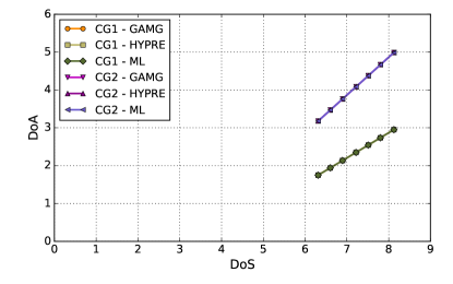
(a) Mesh-convergence

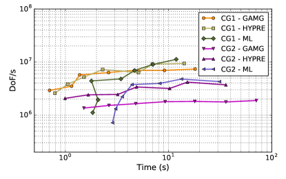
(b) Static-scaling

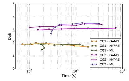
(c) DoE

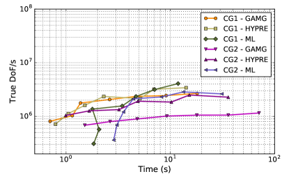
(d) True static-scaling

Figure 13. Test #4: A complete TAS spectrum analysis of different parallel multigrid solvers across 1024 MPI processes.

Table 6 contains the DoA and DoS information for CG1 and CG2. As seen from the FEniCS/Dolfin, Firedrake, and deal.II libraries, the higher order methods have larger DoA/DoS ratios. The complete TAS spectrum is shown in Figure 13. First, we verify from the mesh convergence diagram that the solutions obtained from each solver for a range of $h$-sizes have the expected $\alpha/d$ slopes. Second, the static-scaling diagram shows how the results for each finite element discretization are heavily influenced by the solver. Although the ML solver experiences the most significant strong-scaling effects, it has the highest peak DoF per second rate for both CG1 and CG2. Another observation that can be made from this diagram is that the GAMG solver has the flattest line, indicating the best scalability in the strong scaling limit, but it is the least efficient in terms of processing its DoF. Of course, the data could change if one were to optimize the solver parameters for this problem. It can be also be seen that CG1 has the higher DoF per second rates, but the DoE diagram indicates that CG2 is actually more efficient. The lines in this diagram are not completely straight due to the strong-scaling effects previously noted. Lastly, it can be seen that both CG1 and CG2 are grouped closely together in the true static-scaling diagrams, suggesting that both discretizations are processing the scaled DoFs at an equal pace. Overall, the TAS spectrum analysis tells us that CG2 is the more efficient algorithm to use under the PETSc DMPlex framework, and the choice of solver would depend on problem size.

6. Conclusion

By incorporating a measure of accuracy, or convergence of the numerical method, into performance analysis metrics, we are able to make meaningful performance comparisons between different finite element methods for which the worth of an individual FLOP differs due to different approximation properties of the algorithm—whether because of differences in discretizations, convergence rates, or any any other reason. For example, we saw that for the 3D Poisson problem with smooth coefficients, the DG1 method may have the highest computation rate in terms of DoF per time but have low DoE and true DoF per time metrics once DoA is taken into consideration. Simultaneously looking at the DoE and true DoF per time diagrams can further the understanding of how fast and accurate a particular method is.

6.1. Extensions of this work

The Time-Accuracy-Size (TAS) spectrum analysis opens the door to a variety of possible performance analyses. The most logical extension of this work would be to to analyze different and more complicated PDEs, but there still exist some important issues that were not covered in this paper. We now briefly highlight some of these important areas of future research:

• Arithmetic intensity: A logical extension of the TAS spectrum performance analysis would be to incorporate the Arithmetic Intensity (AI), used in the performance spectrum [16] and roofline performance model [40]. The AI of an algorithm or software is a measure that aids in estimating how efficiently the hardware resources and capabilities can be utilized. The limiting factor of performance for many PDE solvers is the memory bandwidth, so having a high AI increases the possibility of reusing more data in cache and lowers memory bandwidth demands. It can be measured in a number of ways, such as through the Intel SDE/VTune libraries or through hardware counters like cache misses.

• Numerical discretization: This paper has solely focused on the finite element method using CG and DG discretization, so it would be a worthy research endeavor to investigate other types of elements like hybrid or mixed elements. Furthermore, this type of analysis is easily extendible to other numerical methods like the finite difference, finite volume, spectral element, and boundary integral methods.

• Accuracy measures: The accuracy rate metrics were based on the $L_{2}$ error norm, but other measures of accuracy or convergence, like the $H^{1}$ error seminorm, can be used. The accuracy of different numerical methodologies may sometimes require more than just the standard $L_{2}$ error norm. For example, one can validate and verify the performance of finite element methods for porous media flow models using the mechanics-based solution verification measures described in [38].

• Solver strategies: Only the multigrid solvers HYPRE, GAMG, and ML have been used for the experiments in this paper but there are various other solver and preconditioning strategies one can use which may drastically alter the comparisons between the CG and DG methods. A thorough analysis and survey of all the appropriate solver and preconditioning combinations may be warranted for any concrete conclusions to be made about these finite element methods. There are also different ways of enforcing constraints or conservation laws, solving nonlinear systems with hybrid and composed iterations, and handling coefficient jumps in different ways. For this, we may also want to incorporate statistics of the iteration involved [34].

• Large-scale simulations: The computational experiments performed in the previous section are relatively small, but they can easily scale up so that up to 100K or more MPI processes may be needed. Furthermore, even if smaller scale comparisons were to be made such as the ones shown in this paper, the choice of hardware architecture could play an important role in the scaling analyses. Intel systems were used to convey some important performance comparisons, but such comparisons may be very different on systems provided by IBM, AMD, or even NVIDIA.

References

- [1] M. F. Adams, Evaluation of three unstructured multigrid methods on 3D finite element problems in solid mechanics, International Journal for Numerical Methods in Engineering, 55 (2002), pp. 519–534.
- [2] M. F. Adams, H. Bayraktar, T. Keaveny, and P. Papadopoulos, Ultrascalable implicit finite element analyses in solid mechanics with over a half a billion degrees of freedom, in ACM/IEEE Proceedings of SC2004: High Performance Networking and Computing, 2004. Gordon Bell Award.
- [3] R. Agelek, M. Anderson, W. Bangerth, and W. L. Barth, On orienting edges of unstructured two-and three-dimensional meshes, ACM Transactions on Mathematical Software (TOMS), 44 (2017), p. 5.
- [4] M. Alnæs, J. Blechta, J. Hake, A. Johansson, B. Kehlet, A. Logg, C. Richardson, J. Ring, M. E. Rognes, and G. N. Wells, The FEniCS project version 1.5, Archive of Numerical Software, 3 (2015), pp. 9–23.
- [5] G. M. Amdahl, Validity of the single processor approach to achieving large scale computing capabilities, in Proceedings of the April 18-20, 1967, Spring Joint Computer Conference, AFIPS ’67 (Spring), New York, NY, USA, 1967, ACM, pp. 483–485.
- [6] D. N. Arnold, F. Brezzi, B. Cockburn, and L. D. Marini, Unified analysis of discontinuous galerkin methods for elliptic problems, SIAM journal on numerical analysis, 39 (2002), pp. 1749–1779.
- [7] S. Balay, S. Abhyankar, M. F. Adams, J. Brown, P. Brune, K. Buschelman, L. Dalcin, V. Eijkhout, W. D. Gropp, D. Kaushik, M. G. Knepley, L. C. McInnes, T. Munson, K. Rupp, B. F. Smith, S. Zampini, H. Zhang, and H. Zhang, PETSc users manual, Tech. Rep. ANL-95/11 - Revision 3.8, Argonne National Laboratory, 2017.
- [8] , PETSc Web page. http://www.mcs.anl.gov/petsc, 2017.
- [9] W. Bangerth, D. Davydov, T. Heister, L. Heltai, G. Kanschat, M. Kronbichler, M. Maier, B. Turcksin, and D. Wells, The deal. ii library, version 8.4, Journal of Numerical Mathematics, 24 (2016), pp. 135–141.
- [10] G. Bercea, A. T. T. McRae, D. A. Ham, L. Mitchell, F. Rathgeber, L. Nardi, F. Luporini, and P. H. J. Kelly, A structure-exploiting numbering algorithm for finite elements on extruded meshes, and its performance evaluation in firedrake, Geoscientific Model Development, 9 (2016), pp. 3803–3815.
- [11] S. C. Brenner and L. R. Scott, The mathematical theory of finite element methods, Springer, 2002.
- [12] J. Brown, Threading tradeoffs in domain decomposition, 2016. SIAM Parallel Processing Conference, To Thread or Not To Thread Minisymposium, https://www.cse.buffalo.edu/~knepley/presentations/SIAMPP2016_1.pdf.
- [13] J. Brown, B. Smith, and A. Ahmadia, Achieving Textbook Multigrid Efficiency for Hydrostatic Ice Sheet Flow, SIAM Journal on Scientific Computing, 35 (2013), pp. B359–B375.
- [14] J. Chang, S. Karra, and K. B. Nakshatrala, Large-scale Optimization-Based Non-Negative Computational Framework for Diffusion Equations: Parallel Implementation and Performance Studies, Journal of Scientific Computing, 70 (2017), pp. 243–271.
- [15] J. Chang and K. B. Nakshatrala, Variational Inequality Approach to Enforce the Non-Negative Constraint for Advection-Diffusion Equations, Computer Methods in Applied Mechanics and Engineering, 320 (2017), pp. 287–334.
- [16] J. Chang, K. B. Nakshatrala, M. G. Knepley, and L. Johnsson, A performance spectrum for parallel computational frameworks that solve PDEs, Concurency: Practice and Experience, (2017).
- [17] B. Cockburn, J. Gopalakrishnan, and R. Lazarov, Unified Hybridization of Discontinuous Galerkin, Mixed, and Continuous Galerkin Methods for Second Order Elliptic Problems, SIAM Journal on Numerical Analysis, 47 (2009), pp. 1319–1365.
- [18] V. Eijkhout, Introduction to High Performance Scientific Computing, TACC, 2014.
- [19] M. S. Fabien, M. G. Knepley, R. Mills, and B. M. Rivieré, Heterogeneous computing for a hybridizable discontinuous Galerkin geometric multigrid method, SIAM Journal on Scientific Computing, (2017). In review.
- [20] R. D. Falgout and U. M. Yang, hypre: A library of high performance preconditioners, in International Conference on Computational Science, Springer, 2002, pp. 632–641.
- [21] D. Gaston, C. Newman, G. Hansen, and D. Lebrun-Grandie, MOOSE: A Parallel Computational Framework for Coupled Systems of Nonlinear Equations, Nuclear Engineering and Design, 239 (2009), pp. 1768–1778.
- [22] J. L. Gustafson, Reevaluating Amdahl’s law, Communications of the ACM, 31 (1988), pp. 532–533.
- [23] M. Homolya and D. A. Ham, A parallel edge orientation algorithm for quadrilateral meshes, SIAM Journal on Scientific Computing, 38 (2016), pp. S48–S61.
- [24] R. M. Kirby, S. J. Sherwin, and B. Cockburn, To cg or to hdg: a comparative study, Journal of Scientific Computing, 51 (2012), pp. 183–212.
- [25] B. S. Kirk, J. W. Peterson, R. H. Stogner, and G. F. Carey, LibMesh: A C++ Library for Parallel Adaptive Mesh Refinement/Coarsening Simulations, Engineering with Computers, 22 (2006), pp. 237–254. http://dx.doi.org/10.1007/s00366-006-0049-3.
- [26] M. G. Knepley, Computational Science I, PETSc, 2017. https://www.cse.buffalo.edu/~knepley/classes/caam519/CSBook.pdf.
- [27] M. G. Knepley and D. A. Karpeev, Mesh algorithms for PDE with Sieve I: Mesh distribution, Scientific Programming, 17 (2009), pp. 215–230. http://arxiv.org/abs/0908.4427.
- [28] M. Lange, M. G. Knepley, and G. J. Gorman, Flexible, scalable mesh and data management using PETSc DMPlex, in Proceedings of the Exascale Applications and Software Conference, April 2015.
- [29] M. Lange, L. Mitchell, M. G. Knepley, and G. J. Gorman, Efficient mesh management in Firedrake using PETSc-DMPlex, SIAM Journal on Scientific Computing, 38 (2016), pp. S143–S155.
- [30] A. Logg, Efficient representation of computational meshes, International Journal of Computational Science and Engineering, 4 (2009), pp. 283–295.
- [31] N. K. Mapakshi, J. Chang, and K. B. Nakshatrala, A scalable variational inequality approach for flow through porous media models with pressure-dependent viscosity, Journal of Computational Physics, 359 (2018), pp. 137–163.
- [32] D. A. May, J. Brown, and L. L. Laetitia, pTatin3D: High-Performance Methods for Long-Term Lithospheric Dynamics, in Proceedings of the International Conference for High Performance Computing, Network, Storage and Analysis, SC ‘14, IEEE Press, 2014, pp. 274–284.
- [33] A. T. T. McRae, G.-T. Bercea, L. Mitchell, D. A. Ham, and C. J. Cotter, Automated generation and symbolic manipulation of tensor product finite elements, SIAM Journal on Scientific Computing, 38 (2016), pp. S25–S47.
- [34] H. Morgan, M. G. Knepley, P. Sanan, and L. R. Scott, A stochastic performance model for pipelined Krylov methods, Concurrency and Computation: Practice and Experience, 28 (2016), pp. 4532–4542.
- [35] F. Rathgeber, D. A. Ham, L. Mitchell, M. Lange, F. Luporini, A. T. McRae, G.-T. Bercea, G. R. Markall, and P. H. Kelly, Firedrake: automating the finite element method by composing abstractions, ACM Transactions on Mathematical Software (TOMS), 43 (2016), p. 24.
- [36] P. A. Raviart and J. M. Thomas, A Mixed Finite Element Method for 2-nd Order Elliptic Problems, in Mathematical aspects of finite element methods, Springer, 1977, pp. 292–315.
- [37] M. Sala, J. J. Hu, and R. S. Tuminaro, ML3.1 Smoothed Aggregation User’s Guide, Tech. Rep. SAND2004-4821, Sandia National Laboratories, 2004.
- [38] M. Shabouei and K. Nakshatrala, Mechanics-based solution verification for porous media models, Communications in Computational Physics, 20 (2016), pp. 1127–1162.
- [39] K. Shahbazi, An explicit expression for the penalty parameter of the interior penalty method, Journal of Computational Physics, 205 (2005), pp. 401–407.
- [40] S. Williams, A. Waterman, and D. Patterson, Roofline: An Insightful Visual Performance Model for Multicore Architectures, Communications of the ACM, 54 (2009), pp. 65–76.