Exploring conservative islands using correlated and uncorrelated noise

Abstract

In this work, noise is used to analyze the penetration of regular islands in conservative dynamical systems. For this purpose we use the standard map choosing nonlinearity parameters for which a mixed phase space is present. The random variable which simulates noise assumes three distributions, namely equally distributed, normal or Gaussian, and power-law (obtained from the same standard map but for other parameters). To investigate the penetration process and explore distinct dynamical behaviors which may occur, we use recurrence time statistics (RTS), Lyapunov exponents (LEs) and the occupation rate of the phase space. Our main findings are as follows: (i) the standard deviations of the distributions are the most relevant quantity to induce the penetration; (ii) the penetration of islands induce power-law decays in the RTS as a consequence of enhanced trapping; (iii) for the power-law correlated noise an algebraic decay of the RTS is observed, even though sticky motion is absent; and (iv) although strong noise intensities induce an ergodic-like behavior with exponential decays of RTS, the largest Lyapunov exponent is reminiscent of the regular islands.

I Introduction

Realistic systems are always coupled to environments. Small effects of the environment on the system can nicely be described using random perturbations (noise). In Hamiltonian systems, noise induces dissipation, can destroy the regular dynamics, and affects transport, to mention few examples. The presence of noise can drastically change the dynamics and some regions of the phase space, unaccessible for the conservative case, can be reached when noise is considered. This occurs in typical mixed phase spaces of two-dimensional (2D) Hamiltonian systems, where the KAM tori can be treated as barriers in the phase space that cannot be transposed Ott (2002). In such cases the presence of noise allows chaotic trajectories to penetrate tori leading to new features and behaviors. In general, the presence of noise can modify the volume of invariant set that are scaled with the magnitude of the noise Mills (2006), can enhance trapping effects in chaotic scattering Altmann and Endler (2010), and can change the escape rate from algebraic to exponential decay in scattering regions Seoane and Sanjuán (2008); Seoane et al. (2009) and from trajectories leaving from inside KAM curves Rodrigues et al. (2010). In addition, noise affects anomalous transport phenomena such as negative mobility and multiple current reversals Yang, B. et al. (2012), enhances the creation and annihilation rates of topological defects Wang and Ouyang (2005) and postpones the onset of turbulence and stabilizes the three-dimensional waves which would otherwise undergo gradient-induced collapse Lu et al. (2008). In systems with spatiotemporal chaos, noise delays and advances the collapse of chaos Wackerbauer and Kobayashi (2007). The effect of noise in one-dimensional systems has already been studied Yoshimoto et al. (1998) as well as its influence on the transition to chaos in systems which undergo period-doubling cascades Crutchfield et al. (1981); Shraiman et al. (1981). For this class of systems was demonstrated that noise can induces the escape from bifurcating attractors Demaeyer and Gaspard (2009).

In this contribution we study the effects of noise on the dynamics of the standard map with mixed phase space adding a sequence of independent random variables that follows three different distributions: Gaussian, uniform and a power-law correlated (PLC) distribution. The motivation to chose such distributions is related to the context of open systems. The Gaussian distribution is connected to thermal baths, the uniform distribution due to its simplicity and the PLC distribution related to a very actual research area of finite and non-Markovian environments Bao (2017); S.A.Abdulack et al. (2014); J. Rosa and M. W. Beims (208), to mention a few. Our results show that, using uncorrelated noise, the resulting dynamics does not depend significantly on the choice of the distribution (Gaussian or uniform), as expected Crutchfield et al. (1982). For a PLC noise, algebraic decays for the recurrence time statistics (RTS) curves were found, even for larger intensities of noise. The standard deviations of the distributions are the relevant quantity to change the dynamics. We also show that strong noise intensities induce an ergodic-like behaviour with exponential decays of RTS; however, reminiscent of the regular islands is still visible in the value of the Lyapunov exponent when compared to the noiseless case.

This work is organized as follows: In Sec. II we present the model as well the distributions used for generate the noise. Analytical results for the stability of central points are also presented. In Sec. III the changes in the phase space will be investigate. In Secs. IV and V the dynamics of the standard map with noise will be treated using RTS and Lyapunov exponent, respectively. The occupation of the phase space as a function of time for each case is presented in Sec. VI and in Sec. VII we summarize our main results.

II Standard map with noise

The model used in this work is the paradigmatic Chirikov-Taylor standard map with additive independent random variable at each time step described by Karney et al. (1982)

$$\begin{array}[]{rcll}p_{n+1}&=&p_{n}+\dfrac{K}{2\pi}\sin(2\pi\hskip 0.56917ptx_{n})+\dfrac{D\xi_{n}}{2\pi}&\hskip 11.38092pt[\mathrm{mod}\hskip 8.5359pt1],\\ x_{n+1}&=&x_{n}+p_{n+1}&\hskip 11.38092pt[\mathrm{mod}\hskip 8.5359pt1],\\ \end{array}$$ (1)

where $x_{n}$ is the position at the iteration $n=0,1,2,\ldots$, and $p_{n}$ its conjugated momentum. $K$ is the nonlinear positive parameter, $\xi_{n}$ is the random variable and $D$, also a positive parameter, controls the intensity of $\xi_{n}$. The random variable was included in the above map in a distinct way from that proposed in Karney et al. (1982). The parameter $K$ is responsible for the changes in the nonlinear dynamics, so that for larger values of $K$ stochasticity is obtained. The map (1) has fixed points at $x_{1}=0$, $p_{1}=0$ and at $x_{1}=1/2$, $p_{1}=0$. Applying the stability condition $|\mathrm{Tr}(\mathbf{J})|<2$ for the trace of the Jacobian matrix Lichtenberg and Lieberman (1992), we find $|2\pm K|<2$, where the upper sign corresponds to $x_{1}=0$ and the lower one to $x_{1}=1/2$. Solving the inequality, the point at $x_{1}=0$ is always unstable since $K$ is positive. Considering $x_{1}=1/2$, we see that for $K<4$ the fixed point is elliptic and for $K>4$ it is hyperbolic. These two cases are shown in Fig. 1, using $K=3.28$ in (a) and $K=4.23$ in (b). For $K=3.28$ the fixed point is stable, while for $K=4.23$ trajectories trace a two hyperbolic branch inside the main KAM torus. For the values of $K$ used in this work the destroyed KAM curves form Cantor sets that eventually trap trajectories for a long time. This is called the sticky effect and is characterized by a power-law decay for the RTS curves Chirikov and Shepelyansky (1984); Artuso (1999); Zaslavsky (2002); Cristadoro and Ketzmerick (2008a).

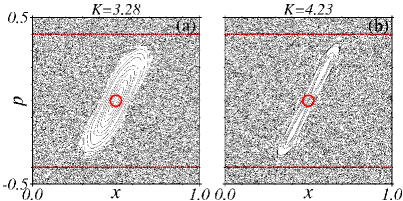
Figure 1: (Color online) Phase-space dynamics for (a) $K=3.28$, and (b) $K=4.23$ using 100 initial conditions and $2\times 10^{5}$ iterations. The fixed points (red circles) localized at $[x,p]=[1/2,0]$ in the center of the figures are (a) elliptic and (b) hyperbolic. Red lines define the border of the chaotic recurrence region to determine the RTS, i.e. above the upper line and below the lower line.

To generate an ensemble of uncorrelated random variables $\xi_{n}$ we choose: (i) the Gaussian (G) distribution [see green plot in Fig. 2(a)] with $\langle\xi_{n}\rangle=0$ and variance $0.22$, to guarantee that $-1\leq\xi_{n}\leq 1$, and (ii) the uniform (U) distribution (see blue plot) for the same range, for which all values of $\xi_{n}$ have the same probability of being picked up. To obtain a correlated noise for $\xi_{n}$ we consider the standard map defined by

$$\begin{array}[]{rcll}I_{n+1}&=&I_{n}+\dfrac{K}{2\pi}\sin(2\pi\hskip 0.56917pt\theta_{n}),\\ \theta_{n+1}&=&\theta_{n}+I_{n+1},\\ \end{array}$$ (2)

where we can define the moment $I_{n}$ between the interval $[-1:1]$ and $\theta_{n}$ in $[0:1]$. Using $K=2.6$, case already studied before Manchein and Beims (2013); da Silva et al. (2015a), we obtain a mixed phase space with KAM curves and a huge stochastic region coexisting. For a given initial condition, the sequence of $I_{n}$ and $\theta_{n}$ near homoclinic points generates a sample of values that obey a time correlated random variable Lichtenberg and Lieberman (1992). Doing $\xi_{n}=I_{n}$, this correlated variable is used here to perturb the map (1). In such cases, the time correlation can be determined from $C(t)=\langle\xi(t)\xi(t^{\prime})\rangle$. For a fully chaotic phase space is expected an exponential decay: $C(t)\propto e^{-b\,t}$ with $t$. However, for a mixed phase space the correlation $C(t)$ presents a power-law tail Meiss et al. (1983); Karney (1983); Chirikov and Shepelyansky (1984); Artuso (1999); Artuso and Manchein (2009), as showed in Fig. 2(b) for $10^{7}$ iterations of map (2). While $C(t)\propto t^{-\delta}$, the RTS curve for this mixed phase space follows $P(\tau)\propto\tau^{-\gamma}$, with $\gamma\sim 1.60$ da Silva et al. (2015a), while $\delta$ and $\gamma$ are related by $\delta=\gamma-1$ Karney (1983); Chirikov and Shepelyansky (1984); Artuso and Manchein (2009). The distribution of $\xi_{n}=I_{n}$, which is PLC, is displayed in Fig 2(a) by the yellow plot.

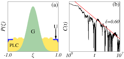
Figure 2: (Color online) (a) Probability Distributions used to generate the random values $\xi$. Gaussian (green), uniform (blue) and PLC noise (yellow), all cases using values inside the interval $[-1:1]$. In (b) we show in logarithm scale the correlation for the variable $I_{n}$ of a standard map for $10^{7}$ time iterations using $K=2.6$ that follows a power-law relation $C(t)\propto t^{-\delta}$.

II.1 Stability condition for the central point

Using $D\neq 0$ in map (1), no periodic orbits exist anymore. However, for one iteration it is possible to analyze the stability of the “fixed point” under the influence of $D$. The “fixed point” at $[x_{1},p_{1}]=[1/2,0]$ is called the central point, and note that it is not a fixed point anymore since the noise changes its location at each iteration. Even though, a one-step stability analysis allows us to demonstrate that the presence of small noise $D\xi_{n}/(2\pi)$ does not change the stability condition of the central point. In fact, for each iteration we are analyzing the one-step stability of a “fixed point”, the central point, whose location changes anytime. The one-step Jacobian matrix $\mathbf{J}_{p}$ of the standard map (1) is given by:

$$\mathbf{J}_{p}=\begin{bmatrix}1&K\cos(2\pi x_{n})\\ 1&1+K\cos(2\pi x_{n})\\ \end{bmatrix}.$$ (3)

The position of the central point is now $p_{1}=0$, $x_{1}=-\frac{1}{(2\pi)}\arcsin[(D\xi_{n})/K]$, and using $\cos[\arcsin(x)]=\sqrt{1-x^{2}}$, the Jacobian $\mathbf{J}_{p}$ becomes

$$\mathbf{J}_{p}=\begin{bmatrix}1&\pm K\sqrt{1-(D\xi_{n})^{2}/K^{2}}\\ 1&1\pm K\sqrt{1-(D\xi_{n})^{2}/K^{2}}\\ \end{bmatrix}.$$ (4)

with eigenvalues $h_{\pm}=\mathrm{Tr}(\mathbf{J}_{p})/2\pm\sqrt{(\mathrm{Tr}(\mathbf{J}_{p})^{2}-4)}/2$, where the trace is given by

$$\mathrm{Tr}(\mathbf{J}_{p})=2\pm\sqrt{K^{2}-(D\xi_{n})^{2}}.$$ (5)

Forcing the eigenvalues of the Jacobian matrix to be $|h_{\pm}|<1$ implies the stability condition $|\mathrm{Tr}(\mathbf{J}_{p})|<2$. Applying this condition to the upper signal, again we have only unstable points for any value of $(D\xi_{n})^{2}$. Considering the lower signal and $K=3.28$ and $K=4.23$, the stability condition for each case remains unaltered for $|D\xi_{n}|\leq 1$, values that will be used in this work. Therefore, all considered noise intensities are not strong enough to change the stability condition for the values of $K$ used here.

III Phase-space dynamics

Plotting trajectories in phase space allows us to identify regions of chaotic and regular motion for the standard map. When noise is included, initial conditions chosen inside the stochastic sea can transpose the barrier of tori and penetrate them. In Fig. 3 the phase-space dynamics are shown for $K=3.28$ in (a)-(i) and $K=4.23$ in (j)-(r). The case with Gaussian noise is displayed in the first line, (a)-(c) and (j)-(l), with uniform noise in the second line, (d)-(f) and (m)-(o), and with PLC noise in the third line, (g)-(i) and (p)-(r). Compared to Fig. 1(a), for $D=10^{-5}$ only some regular trajectories inside the main torus are affected, as we can see in Fig. 3(a), (d) and (g) for $K=3.28$. The most emblematic case is $D=10^{-3}$, for which we have a mixture of completely penetrated tori and other regions still unaccessible. The increasing density of points inside the island from the case $D=0$ indicates that larger sticky motion is expected (this will be shown later). For these cases we can observe that the portion of phase space accessible for the trajectory depends on the distribution used. Using the uniform distribution with $D=10^{-3}$, the trajectories can access most of the phase space, while for the Gaussian distribution there are a lot of regions not visited for same noise intensity. This means that, using distributions for which extreme values of $|\xi_{n}|$ are most likely to occur, it is possible to access a larger portion of the phase space in the same time interval.    

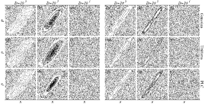
Figure 3: (Color online) Phase space of the map (1) for the interval $(x_{\mbox{\tiny min}},x_{\mbox{\tiny max}})=(0.25,0.75)$, $(p_{\mbox{\tiny min}},p_{\mbox{\tiny max}})=(-0.35,0.35)$ with $K=3.28$ [(a)-(i)] and $K=4.23$ [(j)-(r)] using different intensities of noise indicated above each column. The first line displays the results for Gaussian noise, the second line for uniform noise and the third one for PLC noise. In all simulations we used 100 initial conditions and iterated the map $3\times 10^{5}$ times.

For $D=10^{-1}$, an apparently fully chaotic motion is observed, at least from the phase-space dynamics analysis. However, from the analytical results, we know that the stable central point is still there so that some reminiscent of regular motion is expected. It is worthwhile mentioning here that for a better visualization of the phase-space dynamics we use shorter time iterations when compared to results from Secs. IV, V and VI. However, conclusions made above about the penetration of island should not be substantially changed for longer iterations. Besides, results from the next sections corroborate these findings.

IV Recurrence Time Statistics

In this section we analyze the RTS for the system (1) using different intensities $D$ for each distribution. The RTS is determined numerically by counting the iteration times $\tau$ that the trajectory stays outside of the recurrence region (defined inside the chaotic region). The existence (or not) of the sticky motion is recognized by the cumulative distribution $P_{\text{cum}}(\tau)$ defined by

$$P_{\text{cum}}(\tau)\equiv\displaystyle\sum_{\tau^{\prime}=\tau}^{\infty}P(\tau^{\prime}).$$ (6)

The quantity $P_{\text{cum}}(\tau)$ is a traditional method to quantify stickiness in Hamiltonian Cristadoro and Ketzmerick (2008a); Artuso (1999); Altmann and Kantz (2007); Shepelyansky (2010); da Silva et al. (2015b) and conservative three-dimensional systems da Silva et al. (2015a), since events with long times $\tau$ in the RTS are associated to times for which the trajectory was trapped to the nonhyperbolic components of the phase space. $P_{\text{cum}}(\tau)$ can be directly related with escape time distributions by applying the ergodic theory of transient chaos in systems with leaks Altmann and Tél (2008, 2009). Although there is no general rule, algebraic decays of $P_{\text{cum}}(\tau)$ for at least two decades indicate the existence of sticky motion. When noise is added in Hamiltonian systems with mixed phase space, a slow additional algebraic decay of RTS curves Altmann and Endler (2010); Chirikov and Shepelyansky (1984) and survival probability inside domains near the fixed point Kruscha et al. (2012) was observed, which means that the trapping around regular islands is enhanced due to trajectories that wander inside the islands. This result was also found in a two-dimensional conservative map coupled to an extra dimension without noise. In this case, trajectories remain trapped to the extra dimensional action variable, and for very long times no recurrence occurs, resulting in plateaus in the RTS curves da Silva et al. (2015a). In this section, our focus is to study the relation of enhancing trapping due to $D$ and the kind of distribution used, as well the influence of the stability condition of the central point of the standard map.

The RTS plots for $K=3.28$ are presented in Fig. 4(a)-(c). For the recurrence box we use the chaotic region, displayed in Fig. 1. It can be shown that our results are essentially independent on the choice of the recurrence region, as long it is located inside the chaotic region Sala et al. (2016). For $D=0$ we observe the usual algebraic decay $P_{\text{cum}}(\tau)\propto\tau^{-\gamma}$ with $\gamma=1.55$, indicating the well known sticky motion. For $D\geq 10^{-2}$ no events with long recurrence times exist anymore, and the characteristic long tail of RTS gives place to an exponencial decay, a characteristic of ergodic systems. The enhanced trapping, characterized by a slower algebraic decay ($\varepsilon=0.65$), is present for $D$ inside the interval $[10^{-5}:10^{-3}]$ and for all distribution. This is a consequence of the trapped motion inside de island from the $D=0$ case, as observed by the larger density of point in Fig. 3(b), (e) and (h). Since the trajectory is inside the island, there is a probability of occurring a sequence of $D\xi_{n}$ that keeps the trajectory trapped so that long times of recurrences are reached. The slower decay of the RTS curves means a decrease in the number of recurrences in this interval. Looking at Fig. 4(c), the case for which a PLC noise was used, even for $D=1$ a power-law regime is obtained for the RTS curve, what does not occur for other distributions. The decay follows $P_{\text{cum}}(\tau)\propto\tau^{-\beta}$, with $\beta=2.0$, which characterizes a superdiffusive motion on phase space. It is also interesting to note that for $D=10^{-3}$ and $D=10^{-2}$ in Fig. 4(c) there is an exponential decay for long times and, increasing the intensity $D$, the algebraic decay is recovered. This suggests that the dynamics of the auxiliar map (2) has great influence on the dynamics of map (1) due the relation $D\xi_{n}=DI_{n}$.

The case $K=4.23$ is displayed in Figs. 4(d)-(f). By comparison with $K=3.28$, the enhanced trapping is not that efficient. The reason for this is that the region of sticky motion is smaller, as observed in Fig. 3(k), (n) and (q). Besides that, there is a hyperbolic fixed point inside the main KAM torus forcing the trajectory to stay away from the center. In this case we do not find algebraic decay for RTS curves when using a PLC noise for larger values of $D$. Thus the sticky motion coming from the PLC is not able to significantly keep the sticky motion from the map (1) when the central point is unstable. Another important conclusion is that the RTS curves obtained for $K=3.28$, as well as for $K=4.23$, do not present relevant changes using Gaussian distribution or uniform distribution.    

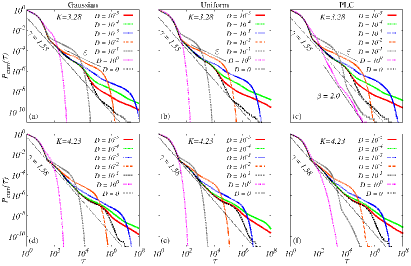
Figure 4: (Color online) Cumulative distribution $P_{\text{cum}}(\tau)$ for recurrence times $\tau$ to a region in the chaotic component of the phase space using Gaussian, uniform and PLC noise distributions, as indicated by the title on the top of each panel with $K=3.28$ and $K=4.23$ for the first and second lines of the figures, respectively. The small algebraic decay $\varepsilon=0.65$ is related to the trapped motion, or enhanced trapping inside the island, and $\beta=2.0$ to the superdiffusive motion.

V Lyapunov exponent

The quantity which measures the average divergence of nearby trajectories is the Lyapunov exponent (LE) $\lambda$, which provides a computable measure of the degree of stochasticity for a trajectory. A numerical method for computing all $2N$ LEs (namely, the Lyapunov spectrum) in a $N$ degrees of freedom system can be found in Benettin et al. (1980); Wolf et al. (1985). This method includes the Gram-Schmidt reorthonormalization procedure. For a randomly perturbed system the technique to compute the Lyapunov spectrum is similar and we just replace the deterministic trajectory $\boldsymbol{x}$ by the perturbed sequence $\boldsymbol{x}^{(p)}$ Crutchfield et al. (1982); Mayer-Kress and Haken (1981). Considering the system studied in this work, since the noise $\xi_{n}$ is independent of $x_{n}$ and $p_{n}$, the fluctuations will not affect the angles between expansion and contraction directions in the tangent space, known as the angles between Lyapunov vectors M.W.Beims and J.A.C.Gallas (2016a, b), but just the probability distributions of variables.

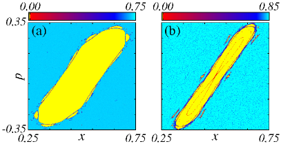
Figure 5: (Color online) The largest LE $\lambda_{1}$ for the map (1) with $D=0$ using a grid of $10^{3}\times 10^{3}$ initial conditions for (a) $K=3.28$ and (b) $K=4.23$. For each trajectory, $\lambda_{1}$ was calculated using $2\times 10^{6}$ time iterations.

To identify changes in the dynamics of the standard map with noise, we divide the phase space of the map (1) for $K=3.28$ and $K=4.23$ in a grid with $10^{3}\times 10^{3}$ points. Each point is an initial condition $[x_{0},p_{0}]$. For trajectories starting at each combination of $[x_{0},p_{0}]$, the largest LE $\lambda_{1}$ was determined using $2\times 10^{6}$ time iterations and is codified by a gradient of colors in Fig. 5 (see the color bar). Clearly, we observe that initial conditions inside the regular islands have $\lambda_{1}\sim 0.0$ (yellow points), with exception the unstable point in Fig. 5(b) with small positive values of $\lambda_{1}$ (red points). Initial conditions related to the chaotic trajectory have larger values of $\lambda_{1}$ (blue and cyan points).    

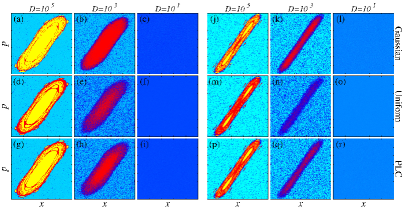
Figure 6: (Color online) The largest LE $\lambda_{1}$ for the map (1) with $K=3.28$ [(a)-(i)], codified by the same gradient color used in Fig. 5(a), and $K=4.23$ [(j)-(r)], codified by the same gradient color used in Fig. 5(b). The first line was obtained using the Gaussian noise, the second line using uniform noise and the third line using the PLC noise. The value of $D$ for each case is indicated above the correspondent column.

If a perturbed trajectory $\boldsymbol{x}^{(p)}$ is considered, as the intensity $D$ of noise increases, sensitive changes can be observed in the value of $\lambda_{1}$ that are displayed in Fig. 6(a)-(i) for $K=3.28$ and (j)-(r) for $K=4.23$, using the Gaussian noise on the first line, uniform noise on the second line, and the PLC noise on the third. The first observation is that by increasing the values of $D$ the islands are penetrated and destroyed in all cases. For $D=10^{-1}$ (Figs. 6(c), (f) and (i) for $K=3.28$ and (l), (o) and (r) for $K=4.23$), the phase space becomes totally chaotic and the same value of $\lambda_{1}$ is obtained for all initial conditions. In other words, the phase space becomes ergodic-like and exponential decays are expected for the RTS curves, as observed in Section IV. The relevant point here is to analyze how the dynamics became ergodic-like using distinct distributions. The Gaussian distribution does not considerably affects the trajectory for small values of $D$ when compared to the other distributions. This becomes evident when comparing the yellow region (or red) from Figs. 6(a), (d), (g), [the same for (j), (m) and (p)] that display the case $D=10^{-5}$ for the Gaussian, uniform, and PLC noise, respectively. The amount of yellow (red) points is larger (smaller) in Figs. 6(a) and (j). Besides, it is interesting to observe that when trajectories penetrate the islands due to noise, they tend to stay close to hyperbolic points from the tori transforming the dynamics more unstable (yellow $\to$ red).

Looking at the case $D=10^{-3}$, Figs. 6 (b), (e) and (h) for $K=3.28$ and (k), (n) and (q) for $K=4.23$, it is possible to note that there are no more initial conditions that lead to stable trajectories (yellow points). Using the uniform distribution [Figs. 6(e) and (n)] higher values $\lambda_{1}$ ($\geq 0.5$) are obtained inside the regular islands from the noiseless case. In addition, looking at the case $K=4.23$, an important result is the fast increasing of $\lambda_{1}$ for initial conditions around the central point, while for the stable case $K=3.28$ the nearby of the central point is kept regular for reasonable values of $D$.

To finish this section, we would like to mention that for the ergodic-like case $D=10^{-1}$, already discussed above, the values of $\lambda_{1}$ are smaller than those obtained for the chaotic trajectory from $D=0$, which is represented as cyan. In other words, instead of increasing the values of $\lambda_{1}$ from the chaotic trajectory, the random distributions allow the total penetration inside the islands and traces of the regular motion are still visible in the asymptotic values of $\lambda_{1}$. Thus, the phase space of the ergodic-like case, which has an exponential decay of the RTS and is totally chaotic, still is influenced by some properties of the destroyed islands. This is true for correlated and uncorrelated distributions and independent of the presence of the stable or unstable central point.

   

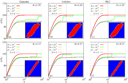
Figure 7: (Color online) Percentage of the phase-space occupied area $A(\%)$ as a function of time for the three distributions and (a)-(c) $K=3.28$ and (d)-(f) $K=4.23$ for some values of $D$. The inset of each case shows the region visited by the trajectory. Blue points represent the visited region for $D=0$, blue$+$yellow points represent the area visited for $D=10^{-5}$ and blue$+$yellow$+$red is the region visited by the trajectory for $D=10^{-1}$, all cases after $10^{8}$ time iterations.

VI Phase-space occupation

The last analysis presented in this work is the occupation rate of the phase space as the intensity $D$ increases. In Fig. 7, the percentage of visited area $A(\%)$ of the phase space is displayed as function of the number of iterations $n$ for some values of $D$. Using $D=10^{-1}$ it is possible to access $100\%$ of the phase space after $n\approx 7\times 10^{6}$ time iterations for any distribution (see the red curves in all panels of Fig. 7).

For $D=10^{-3}$ the whole phase space is occupied just for $K=4.23$ [Fig. 7(d)-(f)], while for $K=3.28$ [Fig. 7(a)-(c)] it is possible only when the uniform distribution is used, and the whole phase space is visited after $n\approx 2.8\times 10^{7}$ iterations [see the green curve in Fig. 7(b)]. In this case, the abrupt increases of $A(\%)$ means that the penetration inside the island is also almost abrupt and not asymptotic.

When the cases $D=0$ and $D=10^{-5}$ are compared, small differences are observed and we need to look at the insets that display the visited area of the phase space for different values of $D$. In all insets, blue points represent the region visited by the trajectory for $D=0$ and blue$+$yellow points represent the region visited for $D=10^{-5}$, both cases after $10^{8}$ iterations. Therefore the case $D=10^{-5}$ allows trajectories to access the high order resonances located around the main torus, what is prohibited for $D=0$, resulting in a small difference between the area occupied in each case. For some intervals of time the trajectory can be trapped in these small island and the visited area for $D=10^{-5}$ (yellow curves) can be smaller than the case $D=0$ (blue curves), as we can see in Figs. 7(d) for $n\approx 1.6\times 10^{6}$ and (f) for $n\approx 1.8\times 10^{7}$. It is important to emphasize that these results are obtained using the initial condition $x_{0}=0.159146$, $p_{0}=-0.470110$, localized in the chaotic sea. If other values are used, the curves may changed slightly but the main conclusions remain unaltered.

VII Conclusions

To summarize, we study the effects of perturbing the standard map randomly using an additive variable $\xi_{n}$ that can follow a Gaussian, a uniform and a PLC distribution. This last one was generated using the deterministic standard map with mixed dynamics. For all distributions, the RTS demonstrates that sticky motion is enhanced for small values of the noise intensity, namely $10^{-5}\leq D\leq 10^{-4}$. The power-law exponent characterizing this decay is $\varepsilon=0.65$. Here the noise tends to increase hyperbolic points from the rational tori from the noiseless case. For intermediate values, $10^{-3}\leq D\leq 10^{-2}$, power-law decays with the same $\varepsilon$ are observed for earlier times, but followed asymptotically by exponential decays. This reflects the fact that larger noise intensities allow an earlier penetration of the island and the time correlation decays faster, i.e, the system becomes ergodic-like for earlier times when compared to smaller noise intensities.

For $D=10^{-1}$, all (with one exception) RTS curves decay exponentially and an ergodic-like motion is expected. However, the largest Lyapunov exponent is smaller when compared to the Lyapunov exponent from the noiseless case. This means that reminiscent of the sticky motion due to the destroyed islands is still affecting the chaotic dynamics. The mentioned exception occurs when a PLC noise is used and $K=3.28$. In this case we found an algebraic decay with $\beta=2.0$, which represents a superdiffusive motion through the island. In fact, with these results it is pretty clear that the most relevant quantity to allow penetration of the island is the standard deviation of the distributions.

Another issue considered in this work was the stability condition for the central point of the phase space. To compare the two possible conditions we study the influence of noise on the standard map for two different values for the nonlinearity parameter: $K=3.28$, for which the central point is stable, and $K=4.23$, for which the central point is unstable. The RTS curves from the Section IV demonstrate that, in the presence of noise, the two cases behave similarly but the transition to stochasticity, when increasing $D$, is faster for the unstable case.

To finish, we would like to relate our results to higher-dimensional systems. Noise can be interpreted as the net effect of extra dimensions. If the dynamics of the extra dimensions is chaotic, the Gaussian distribution is a nice description of such dynamics. If the dynamics of the extra dimensions behaves like a conservative system with mixed phase space, then the PLC distribution should be adequate to describe the net effect. In this context, the global structure of regular tori in a generic $4$D symplectic map was analyzed Lange et al. (2014) and, recently, the decay of RTS was studied to give a nice explanation about the island penetration through one extra dimension da Silva et al. (2015a).