Spectra of Hydrogen-Poor Superluminous Supernovae from the Palomar Transient Factory

Abstract

Most Type I superluminous supernovae (SLSNe-I) reported to date have been identified by their high peak luminosities and spectra lacking obvious signs of hydrogen. We demonstrate that these events can be distinguished from normal-luminosity SNe (including Type Ic events) solely from their spectra over a wide range of light-curve phases. We use this distinction to select 19 SLSNe-I and 4 possible SLSNe-I from the Palomar Transient Factory archive (including 7 previously published objects). We present 127 new spectra of these objects and combine these with 39 previously published spectra, and we use these to discuss the average spectral properties of SLSNe-I at different spectral phases. We find that Mn II most probably contributes to the ultraviolet spectral features after maximum light, and we give a detailed study of the O II features that often characterize the early-time optical spectra of SLSNe-I. We discuss the velocity distribution of O II, finding that for some SLSNe-I this can be confined to a narrow range compared to relatively large systematic velocity shifts. Mg II and Fe II favor higher velocities than O II and C II, and we briefly discuss how this may constrain power-source models. We tentatively group objects by how well they match either SN 2011ke or PTF12dam and discuss the possibility that physically distinct events may have been previously grouped together under the SLSN-I label.

1 Introduction

The highest luminosity supernovae (SNe), often called “superluminous supernovae” (SLSNe; Gal-Yam 2012), are of special interest because they mark the upper extremum of stellar explosions, can be detected out to very high redshifts ($z$), and may be used to probe the early universe. SLSNe may derive their luminosity from unique power sources or from processes that make only minor contributors to normal SNe (Kasen & Bildsten, 2010; Woosley, 2010; Chevalier & Irwin, 2011), and some may offer important constraints on the final stages of stellar evolution (Woosley, 2017). SLSNe may further have applications in cosmology (Inserra & Smartt, 2014; Scovacricchi et al., 2016), studies of the stellar initial mass function (Tanaka et al., 2012), and probing the metal content of early star-forming regions (Berger et al., 2012; Vreeswijk et al., 2014); moreover, they may provide a means to directly study the first stars (Whalen et al., 2013). But to confidently use SLSNe as probes of the high-redshift universe, we must build a better physical understanding of these stellar explosions and identify what it is exactly that distinguishes these events from normal-luminosity SNe so that we can account for any evolution with redshift.

Observationally, SNe are sorted into a number of different types primarily by their spectra (Filippenko, 1997; Gal-Yam, 2016). A supernova (SN) is classified as Type II if it exhibits obvious hydrogen features in spectra taken near maximum light, Type Ia if hydrogen is lacking but Si II is strong, Type Ib if hydrogen is lacking, Si II is weak, and helium lines are well detected, and finally Type Ic if none of these classifications hold (we will use SN II, SN Ia, SN Ib, and SN Ic to refer to these spectral types, respectively; see Fig. 1). There are further refinements of this classification scheme for objects with relatively narrow emission features (SN IIn and SN Ibn), transitional objects (e.g., SN IIb), and sometimes objects are subclassified by their light-curve properties (e.g., SN II-P and SN II-L).

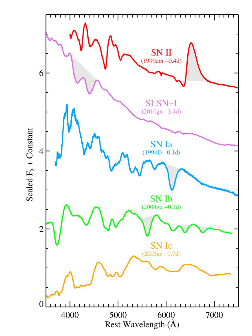
Figure 1: Spectra near peak optical brightness of a SLSN-I compared to normal-luminosity SNe. Some key features are shaded in gray for emphasis: H I in the SN II, O II in the SLSN-I, Si II in the SN Ia, and He I in the SN Ib. Except for SN 1994D, the data have been smoothed for clarity.

Normal SNe typically have optical luminosities in the $-14<M<-20$ mag range (Li et al., 2011; Richardson et al., 2014). The SLSN label has traditionally been assigned to events with peak absolute magnitudes brighter than about $M<-21$ in the optical (Gal-Yam, 2012). Many papers have been published on specific SLSN events (e.g., Hatano et al. 2001; Smith et al. 2007; Quimby et al. 2007a; Gal-Yam et al. 2009; Barbary et al. 2009; Quimby et al. 2011; Chomiuk et al. 2011; Rest et al. 2011; Leloudas et al. 2012; Howell et al. 2013; Nicholl et al. 2014; Benetti et al. 2014), and there is a growing number of papers exploring the diversity of the population (e.g., Inserra et al. 2013; Nicholl et al. 2015; Lunnan et al. 2017; De Cia et al. 2017). The SLSN group may now include over 100 distinct events (Guillochon et al., 2017), but this is just 0.26% of all reported SNe — a testament to the low volumetric rates at which SLSNe are produced (Quimby et al., 2013; Prajs et al., 2017).

SLSNe with obvious spectroscopic evidence for hydrogen near maximum light have been classified as SNe II (or SLSNe-II to highlight their extreme luminosities), while others lack the defining features noted above and fall into the default SN Ic (or SLSN-I) category. Some initially hydrogen-poor SLSNe develop hydrogen features in their later-time spectra (Yan et al., 2015, 2017b), although these are usually classified as SLSNe-I. Additionally, a SLSN-R class has been introduced (Gal-Yam, 2012), but this may not be distinct enough from SLSNe-I to warrant a separate class (De Cia et al., 2017).

Since the first examples were published a decade ago, the physical nature of these objects has been debated. Models developed to explain normal-luminosity events ($M>-20$ mag) cannot easily be stretched to account for the immense energies released by SLSNe (the radiation budgets alone can exceed $10^{51}$ erg; e.g., Chatzopoulos et al. 2011), so new power sources have been sought.

Among the first models to be considered were the pair-instability explosion models that had been developed to predict the deaths of the first stars (Fowler & Hoyle, 1964; Barkat et al., 1967). These models initially assumed zero-metallicity progenitors, but they have been compared to explosions in the $z\approx 0$ universe (e.g., Smith et al. 2007; Gal-Yam et al. 2009). Not all agree that these models explain the data, however (e.g., Dessart et al. 2012; Jerkstrand et al. 2017). Nonetheless, recent developments in stellar evolution theory incorporating rotation have pointed to possible avenues for stars with the required, extremely-massive cores to exist in the modern universe (Yoon & Langer, 2005; Woosley & Heger, 2006; Yusof et al., 2013), and this is supported by observations (Crowther et al., 2016), so this progenitor model continues to be explored (e.g., Whalen et al. 2014; Kozyreva et al. 2017).

Most of the hydrogen-rich SLSNe-II show time-variable, narrow emission lines in their spectra that indicate a relatively slow-moving wind is being overtaken by fast-moving ejecta (e.g., Fransson et al. 1996). This interaction potentially offers an additional source of power that may help to explain their high luminosities (e.g., Smith et al. 2007; Chatzopoulos et al. 2011; Chevalier & Irwin 2011). SLSNe-I do not exhibit these tell-tale spectral features (e.g., Pastorello et al. 2010; Quimby et al. 2011; Inserra et al. 2013). However, SLSNe-I may yet be powered by interaction if the wind is very extended and moving at a high velocity (Chatzopoulos & Wheeler, 2012), or if the wind is depleted of hydrogen and not photoionized by the SN (see, for example, the helium or carbon-oxygen wind models of Tolstov et al. 2017a). SLSNe-I also show somewhat weak spectral features from relatively cool ions that may be diluted by a hot continuum produced by an underlying interaction (Chen et al., 2017). But the lack of obvious interaction signatures opens the possibility that different SLSNe are powered primarily through different means (or that the signs of interaction in most SLSNe-II are a red herring).

An attractive explanation for the unusually high energies of SLSNe-I is that additional energy is deposited in the ejecta over time as a nascent magnetar spins down (Kasen & Bildsten, 2010; Woosley, 2010). Although the details are lacking on how this spindown energy is injected into the ejecta, the bolometric evolution of several SLSNe-I has been fit with this model yielding a plausible range of initial spin periods, magnetic fields, and ejecta masses (Inserra et al., 2013; Liu et al., 2017; Nicholl et al., 2017b). Although the light curves of some SLSNe-I can be fit with the magnetar model, other power sources have been shown to fit certain events as well or better (Chatzopoulos et al., 2013), and thus photometry alone has not ended the debate over what powers SLSNe-I.

However, there are other potential tests to discriminate between SNe powered internally from magnetar spindown or centrally located ⁵⁶Ni, externally from the outer ejecta interacting with slower-moving material, or from a combination of magnetar, ⁵⁶Ni, and interaction power sources. The wealth of information provided through spectroscopy may hold the key to separating these models. For example, if SLSNe are powered primarily by an exceptionally large yield of ⁵⁶Ni, the spectra may show evidence for an unusually large amount of iron-peak elements (Dessart et al., 2012). Moreover, if energy is added from within, then this could change the velocity structure of the ejecta by accelerating the slowest-moving material in the interior and forming a bubble of evacuated space, similar to a pulsar wind nebula (Metzger et al., 2014). The interaction model can similarly result in a shell-like structure, but in this case the interior velocity structure should retain the homologous expansion velocities rendered from the explosion. Thus, the velocity evolution and the final velocity distribution at late times may serve to distinguish the magnetar model from the interaction model.

To determine the velocity structure of the ejecta, the ions responsible for the spectroscopic features must be properly identified. Significant work has been done on identifying the features in normal-luminosity SN spectra, but the application of this work to SLSNe-I is complicated by two issues: (1) the strength of spectral features tends to be much lower in SLSNe-I than in SNe Ic (e.g., see Fig. 1), and (2) owing to ionization and possibly composition differences, there are likely features in the SLSN-I spectra that are not present in normal-luminosity SNe, and these may blend with or totally dominate the normal features. The latter is certainly true for the O II ion, which dominates the optical spectra of most young SLSNe-I (Quimby et al., 2011) but which is not typically seen in lower-luminosity events; two notable exceptions, SN 2008D (Soderberg et al., 2008; Mazzali et al., 2008; Modjaz et al., 2009) and OGLE-2012-SN-006 (Pastorello et al., 2015), are discussed below. These features offer the only means to extract velocity information from the spectra in some cases — but, unfortunately, these features are the product of many blended lines (Mazzali et al., 2016), and a simple method for extracting velocity information from them has yet to be developed.

The connection between normal-luminosity SNe Ic and SLSNe-I may also help constrain the source of power. The nascent magnetars may serve a wide range of power to the SN ejecta depending largely on the initial spin period and magnetic-field strength (Kasen & Bildsten, 2010; Woosley, 2010). Many of these combinations may result in relatively low spindown luminosities. Because SLSNe have traditionally been selected by their luminosities (e.g., Gal-Yam 2012), there may be an artificial division between the fainter SNe that come from these conditions and the high-luminosity objects that result from more optimal initial conditions, even though the two are physically related. However, if such a power source is present and significant, then the velocity and perhaps ionization evolution may still be detectable in the lower-luminosity events. Yet to discover this connection, a method to identify SNe physically similar to SLSNe-I but with lower luminosities must be developed.

In this paper, we discuss a method to select objects spectroscopically similar to the published sample of SLSNe-I independent of their light curves. We show in §2 that although at certain light-curve phases SLSNe-I have spectral features that are similar to those of normal-luminosity SNe Ic at other light-curve phases, the spectra of SLSNe-I tend to be better matched to the spectra of other SLSNe-I (and not SNe Ic) over a wide range of phases. The two groups can thus be spectroscopically divided. In §3 we apply this classification scheme to the spectra of 1815 SNe discovered by the Palomar Transient Factory and present 19 objects that are best classified as SLSNe-I and an additional 4 objects that are possibly SLSNe-I. In §4 we consider 133 spectra of SLSNe-I taken over a variety of phases. These spectra are organized into a sequence and we assign spectral phases, $\phi$, to SLSN-I and SN Ic spectra by matching these data to our SLSN-I sequence. We also discuss in this section the clustering of objects as more similar to PTF12dam or SN 2011ke. In §5 we compare the mean spectral properties of SN 2011ke-like and PTF12dam-like events at four different spectral phases and note some potential differences. Individual spectra are examined in §6 to identify line features. We pay particular attention to O II, identify Mn II with high probability for the first time, and note the presence of obvious hydrogen and helium lines in PTF10aagc and PTF10hgi, respectively. With secure line identifications in hand, we present the O II and Fe II velocity evolution of PTF12dam in §7. We discuss our findings and provide a summary of our conclusions in §8.

2 Spectroscopic Selection of SLSNe-I

SNe are usually classified by matching their spectral features to objects of known types. There are three different techniques used for spectral matching of SNe: $\chi^{2}$ minimization, cross correlation, and “feature” matching in a series of wavelength bins (e.g., Riess et al. 1997; Harutyunyan et al. 2008). We choose to use the $\chi^{2}$ minimization routine, superfit (Howell et al., 2006), for our main analysis and we test our findings using a custom cross-correlation code based on SNID (Blondin & Tonry, 2007). Briefly, superfit compares an input spectrum to a library of template SN spectra. Each template is reddened (or dereddened) using a Cardelli extinction law (Cardelli et al., 1989), a galaxy template is added to account for any host-galaxy contamination, and the $\chi^{2}$ value of the model fit is determined. The templates are then rank ordered by their $\chi^{2}$ values. We describe below how we build our comparison spectral library, account for the varying rest-frame wavelength coverage of these templates, and then interpret the match results to derive a final spectral classification for an input object.

2.1 Spectral Template Library

The library of template spectra used for the fitting is naturally an important concern. In principle, it would be best to have theoretical models with uniform wavelength and phase coverage for all possible classes of SNe. However, there are very few models available today that are sufficiently realistic for our needs. We are thus forced to base our spectral templates on observations.

For our analysis, we constructed a new library of spectral templates based on observations. For the SNe Ia, we use the CfA Supernova Archive, which includes 1924 unique observations of 221 SNe Ia with spectroscopic subtypes identified (Blondin et al. 2012; see also the Berkeley Supernova Ia Program, Silverman et al. 2012b). We similarly used the CfA Supernova Archive’s 480 spectra of 44 stripped-envelope core-collapse SNe including Types Ib, Ic, and the more rare Ic-bl, IIb, and Ibn, with light-curve phase information (Modjaz et al., 2014). To these we added 107 well-observed spectra of stripped-envelope core-collapse SNe, as well as 373 spectra of 22 SNe II and SNe IIn, from a number of sources (see Table 1). These data were downloaded from WISeREP (Yaron & Gal-Yam, 2012). In total, our library contains 2884 spectra of normal-luminosity SNe.

Table 1: Spectral Template Libraries

Group	Number of Spectra	References
SNIa	1924	Blondin et al. (2012)
SNII/SNIIn	373	Pun et al. (1995); Leonard et al. (2000); Fassia et al. (2001); Leonard et al. (2002); Pastorello et al. (2004); Fransson et al. (2005); Vinkó et al. (2006); Pastorello et al. (2006); Sahu et al. (2006); Quimby et al. (2007b); Bufano et al. (2009); Pastorello et al. (2009); Stritzinger et al. (2012); Taddia et al. (2013); Bayless et al. (2013); Dall’Ora et al. (2014); Zhang et al. (2014); Takáts et al. (2014); Spiro et al. (2014); Jerkstrand et al. (2014)
SNIb, SNIc, SNIc-bl, SNIbn, SNIIb	587	Barbon et al. (1995); Filippenko et al. (1995); Matheson et al. (2001); Patat et al. (2001); Branch et al. (2002); Foley et al. (2003); Folatelli et al. (2006); Taubenberger et al. (2006); Pastorello et al. (2007); Harutyunyan et al. (2008); Valenti et al. (2008); Pastorello et al. (2008); Malesani et al. (2009); Modjaz et al. (2009); Taubenberger et al. (2009, 2011); Modjaz et al. (2014)
SLSN-I	118	this work; PESSTO-DR1; Quimby et al. (2007a); Barbary et al. (2009); Gal-Yam et al. (2009); Pastorello et al. (2010); Chomiuk et al. (2011); Inserra et al. (2013); Howell et al. (2013)
SLSN-II	22	Smith et al. (2007, 2010); Chatzopoulos et al. (2011)

Table 2: SLSN-I Spectroscopic Reference Set

Name	$z$	$N_{\rm spec}$	Reference
SN 2005ap	0.283	2	Quimby et al. (2007a)
SCP06F6	1.189	3	Barbary et al. (2009)
SNLS-06D4eu	1.588	1	Howell et al. (2013)
SN 2006oz	0.396	1	Leloudas et al. (2012)
SN 2007bi	0.128	3	Gal-Yam et al. (2009)
SNLS-07D2bv	1.500	1	Howell et al. (2013)
PTF09atu	0.501	7	this work, Quimby et al. (2011)
PTF09cwl	0.350	6	this work, Quimby et al. (2011)
PTF09cnd	0.259	13	this work, Quimby et al. (2011)
SN 2010gx (PTF10cwr)	0.230	12	this work, Pastorello et al. (2010), Quimby et al. (2011)
PTF10hgi	0.098	16	this work, Inserra et al. (2013)
PS1-10ky	0.956	4	Chomiuk et al. (2011)
PS1-10awh	0.908	3	Chomiuk et al. (2011)
SN 2011ke (PTF11dij)	0.143	15	this work, Inserra et al. (2013)
SN 2011kf	0.245	2	Inserra et al. (2013)
PTF11rks	0.192	10	this work, Inserra et al. (2013)
SN 2012il	0.175	3	Inserra et al. (2013)
PTF12dam	0.108	28	this work, Nicholl et al. (2013)
LSQ12dlf	0.250	6	Nicholl et al. (2014)
SSS120810	0.156	6	Nicholl et al. (2014)
SN 2013dg	0.265	1	Nicholl et al. (2014)

Next, we need a library of SLSN spectral templates. For these we use 92 publicly available spectra of 20 objects published before early 2015 as SLSNe-I or SLSNe-II. We further include 31 PTF spectra for three of these objects, which we publish here for the first time (see §3). Our SLSN template library is thus based on events that have been classified as SLSNe from their luminosities.

For all of our spectral libraries, we must remove features in the data that do not relate to the SNe, including cosmic rays, telluric features, and narrow spectral lines from gas in the host galaxy. We first remove narrow lines (only those unrelated to the SNe) by fitting Gaussian profiles at the expected locations of typical host-galaxy lines. We perform this fit section by section with all lines in a given section constrained to have the same full width at half-maximum intensity (FWHM) in the fit. We then remove only lines that were significantly detected according to the fit. We also remove telluric features using a high-resolution telluric spectrum degraded to the approximate resolution of the spectra. Given changes in atmospheric conditions this fitting is imperfect, but it can greatly reduce the effects of telluric features in spectral templates for which the reducers have not already removed these features (this practice is unfortunately not standard). We then smooth the templates using a generalized Savitzky-Golay filter as described in Appendix A (this smoothing step was not done for the SN Ia spectra, but a large fraction of these data are high signal-to-noise (S/N) ratio observations that would not benefit from smoothing; e.g., see Fig. 1). For templates lacking error spectra, we estimate the error spectra by fitting out the broad SN features with an iterative B-spline fit. The error is then estimated from the standard deviation of the B-spline-subtracted spectrum in several intervals and then interpolated to the entire spectral range.

2.2 Wavelength Range for Spectral Matching

A significant problem in SN template libraries is that the libraries are constructed from observations and thus do not uniformly cover all of the desired parameter space. First, the libraries include objects at different redshifts and they are observed with different instruments. Thus, the rest-frame wavelength coverage varies significantly from spectrum to spectrum. Second, we have an order of magnitude more SN Ia templates than the other object types. Likely our templates do not account for the full diversity of each class of object (except possibly for the SNe Ia). As discussed below, this may result in false matches with the wrong object type. Third, the templates are by no means evenly distributed with respect to light-curve phase. Gaps in the temporal coverage of one type of object may again lead to matches skewed to another object type with better coverage at the relevant light-curve phase. A final problem of note is that some templates have more noise than others, and some may be contaminated by host-galaxy lines, telluric features, cosmic rays, or other artifacts. Below we discuss how we account for these potential problems.

Figure 2 shows the number of spectral templates in our libraries for different types of SNe as a function of wavelength. Most of the normal-luminosity SNe are low-redshift objects with only ground-based optical coverage; a notable exception is SN 1987A, which has a number of ultraviolet (UV) spectra. Consequently, there are few templates of normal-luminosity SNe with rest wavelengths below about 3500 Å. Spectroscopic coverage of these objects is limited to $\lambda<7500$ Å as well, since this is the effective limit of the FAST spectrograph (Fabricant et al., 1998) at the Fred Lawrence Whipple Observatory, which supplied most of the observations.

Figure 2: Wavelength coverage of our spectral template libraries (number of templates per wavelength bin).

In contrast, SLSNe-I are typically found at significantly higher redshifts (e.g., $z\approx 0.3$); hence, ground-based follow-up observations naturally cover shorter rest-frame wavelengths. The SLSNe-I in the template sample were also more frequently observed with dual-channel instruments offering superior blue and red wavelength coverage. A greater fraction of SLSNe-I thus have coverage below 3000 Å and above 8000 Å than the SN Ia and stripped-envelope core-collapse samples from the CfA archive.

Based on the wavelength coverage of our spectral templates shown in Figure 2 and the spectral features of various SNe shown in Figure 1, we choose to input only the rest-frame 3900–7000 Å range of our test spectra to our template matching codes. This way, templates with better spectral coverage will not be artificially favored. If we did not do this, then a SLSN-I spectrum might be much more likely to match other SLSN-I templates simply because many of the other templates would be rejected owing to insufficient wavelength coverage.

2.3 Automated Template Matching

Typically, the final classification of SN spectra is left to human judgment. Template matching is performed using an automated code, which returns a rank-ordered list of possible matches. However, the top match from the template libraries is not guaranteed to have the same spectral classification as the input spectrum. The input spectrum may be for a subtype or taken at a phase that is missing from the libraries. More generally, the libraries may not fully account for the diversity of SN spectra. Because of this and possible systematic errors in the libraries and input spectra (e.g., imperfect calibration, telluric removal, or the presence of artifacts), template-matching codes serve as imperfect tools that require human oversight.

A disadvantage of human interaction in spectral classification is that it can be subjective. Different groups may disagree with the interpretation of the output from spectral matching codes (for example, see the difference in opinion on the classification of PS1-10afx; Quimby et al. 2013; Chornock et al. 2013). In this work, we favor a classification scheme that is (mostly) free of human interpretation and should thus be readily reproducible by others using the same technique. We show below that although the top match output by a spectral matching code may not always belong to the same class as the input object, it is the case that the top matches belonging to the correct class tend to be systematically higher in the rankings than they would be for input objects of different types. We can thus compare how highly ranked the top matches of each class are and compare the differences in these average scores to a training set to determine the true classification (with quantifiable uncertainty). With a sufficiently large set of library spectra and careful consideration of sample bias, spectral classification can be automated.

With the smoothed spectral template libraries in hand, we can now check if SLSN-I spectra at various phases are equally well matched by SLSN-I and SN Ic templates or if the spectra alone indicate separate populations. To do this test, we input each spectral template individually into superfit and determine how well these spectra match each of the smoothed spectra in our template libraries. For each spectrum we exclude matches to any templates of the same object in our libraries and create a rank-ordered list of the best-matching templates. For this test we artificially redshift the input spectra to $z=0.1$ for convenience. This choice ensures that matches to the SN templates, which include objects spanning a wide range of velocities, will always result in a positive redshift. For the SNe Ia, we use only the elliptical galaxy template to account for host-galaxy contamination (most of the templates have little or no host-galaxy contamination), we set the allowed range of $A_{V}$ from $-2$ to 2 mag, and we fix the redshift search range to $0.07\leq z\leq 0.13$ in steps of $\delta z=0.01$. (Note that the $A_{V}$ parameter is normally intended to account for reddening by the host galaxy, but it can also be used to adjust for intrinsic color differences of SNe themselves; thus, negative values are acceptable.) For all other SNe, we use the Sc galaxy template, allow $A_{V}$ to vary from $-4.5$ to 2 mag, and fix the redshift search range to $0.03\leq z\leq 0.17$ (the larger $A_{V}$ range helps to account for the greater intrinsic color range of this group; see §2.5). These values were selected considering the range of expansion velocities and reddening in our libraries and after a number of superfit trials. As noted earlier, the rest-wavelength range for the input templates is fixed to at most 3900–7000 Å, and we only include templates that cover 95% or more of this wavelength range. All other superfit parameters are left at their default settings.

2.4 Testing the Automated Spectral Classification

In Figure 3, we show that with these settings and our template libraries, we can distinguish the classes of normal-luminosity SNe. The figure shows $\Delta I_{\rm Ic-X}=\langle I_{\rm Ic}\rangle-\langle I_{\rm X}\rangle$, the difference between the average index of the top 5 SN Ic template matches found by superfit, $\langle I_{\rm Ic}\rangle$, minus the average index, $\langle I_{\rm X}\rangle$, for SN Ia, SN Ib, or SN II templates. Here “index” just means the ranking of the template as determined by superfit, with larger indices indicating worse matches. For example, if the top 5 matches found by superfit are all SN Ia templates, then the average index will be $\langle I_{\rm Ic}\rangle=2.0$ (the indices are zero-indexed; that is, the index of the best-matching template is zero.). Lower values for $\Delta I_{\rm Ic-X}$ indicate that the SN Ic templates tend to be more highly ranked. In each case it is apparent that the SNe Ic can be distinguished from the other populations; this is readily confirmed by a formal Kolmogorov-Smirnov (KS) test.

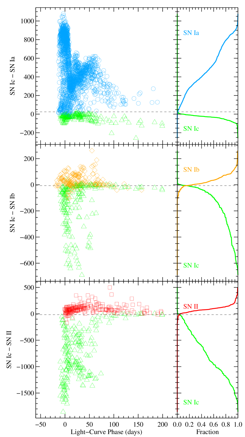
Figure 3: The population of SNe Ic can be separated from SNe Ia, SNe Ib, and SNe II using the difference in the average superfit index of the best-matching templates from our spectral libraries. In each panel, the ordinate is computed by taking the indices of the top 5 matches from the rank-ordered list output by superfit and subtracting the average of these for a given SN type from the average of the top 5 SN Ic indices. Plots in the left column show this index difference as a function of light-curve phase, which is days from explosion for SNe II and days from maximum light for all other types. The plots in the right-hand column show the cumulative fractions of observations with index differences greater than (for the SNe Ic) or less than (for the other types) a given value.

We plot the $\Delta I_{\rm Ic-X}$ values as a function of light-curve phase. This allows us to demonstrate some of the degeneracy between different SN types. For example, SNe Ia are more easily distinguished from SNe Ic at maximum light than they are two weeks later when the Si II line at 6150 Å weakens and the overall appearance becomes more SN Ic-like. The division between SNe Ic and SNe Ib is less distinct especially at later phases, when the helium lines have weakened and the available spectra are limited. Obviously the distinction between classes can be most strongly made in this analysis at phases where there are larger numbers of library templates in each group.

Marginalizing over light-curve phase, we can determine the fraction of spectra with $\Delta I_{\rm Ic-X}$ values less than a given value. The figure shows this for the SNe Ic and the fraction with $\Delta I_{\rm Ic-X}$ greater than the given value. We can then determine the cutoff value where the fraction of SNe Ic above the cutoff equals the fraction of the SNe Ia, SNe Ib, or SNe II below the cutoff. This is shown with the horizontal dashed lines in the figure. For objects with multiple spectra, we can average the results to determine the overall classification. The contamination rate is estimated from the fraction of the populations that are incorrectly classified by this cutoff. For example, for SNe Ic the contamination rates of SNe Ia, SNe Ib, and SNe II are 0.8%, 15.1%, and 3.7%, respectively. We use this cutoff value to classify each object as more SN Ic-like or more like a SN Ia, SN Ib, or SN II.

The final result of this procedure is a calibrated system to classify SN spectra. If we use the same procedures with the same template libraries to find the best matches to a new SN, we can determine the $\Delta I_{\rm Ia-X}$, $\Delta I_{\rm Ib-X}$ (etc.) scores and compare these to our calibrated cutoff scores to find if this new object is most similar to a SN Ia, SN Ib (etc.). The population overlap from the template libraries then gives an indication of how trustworthy this classification is. For example, Figure 3 shows that a $\Delta I_{\rm Ic-Ib}$ score of $-300$ would signify that the object is definitely more SN Ic-like than SN Ib-like (none of the library SN Ib templates scores this low), while a score of $-10$ would indicate an ambiguous classification (11% of the library SNe Ib have $\Delta I_{\rm Ic-Ib}$ scores this low or lower).

We can test this classification system using the template libraries. Of the 302 objects tested (we exclude the SLSNe-II SN 2006gy and SN 2008am), we find 295 (98%) are classified in agreement with the published types by the process described above. Of the 7 that are classified differently, 4 are SNe Ia that are incorrectly classified as SLSNe-I. As discussed below, this is to be expected given the large SN Ia sample and the slight overlap between the populations, but such interlopers can be removed based on other metrics. Another difference is that the lone spectrum of the SN 1991bg-like (peculiar SN Ia; e.g., Filippenko et al. 1992) SN 2006em (González-Gaitán et al., 2011) is found to be marginally more consistent with a SN Ic strictly following our method above (the top superfit matches for this object are all SNe Ia-CL, but there are a few matches to the SN Ic 2004aw relatively high in the ranking that throw off the classification). Additionally, the Type Ic SNe 2004dn and 2005kl are classified as SNe Ib through our method. For the latter, at least Modjaz et al. (2014) find the spectral classification to be ambiguous because data were not taken in the phase when the helium lines are readily visible, so the SN Ib classification may be accurate. However, SN 2004dn was firmly classified as a SN Ic by Sun & Gal-Yam (2017).

2.5 SLSN-I Spectra Differ from Normal-Luminosity Events

Having demonstrated that normal-luminosity SNe can be accurately classified using their $\Delta I_{\rm X-Y}$ scores, we turn to SLSNe. We use the procedure outlined above and test the $\Delta I_{\rm SLSN-I-X}$ values for each of the normal-luminosity types. Given the importance on the number of template library spectra demonstrated above, we deem the 22 SLSN-II spectra insufficient for this procedure. Thus, we cannot automatically distinguish between SLSNe-II and SLSNe-I (or any other type). Lacking this ability, we can still determine if an object is best matched by SLSN-I templates and then visually check for the obvious presence of hydrogen in the spectra to determine if it should properly be classified as a SLSN-II.

Figure 4 shows the $\Delta I_{{\rm SLSN-I}-{\rm X}}$ values for the 118 spectra of confirmed SLSNe-I along with the same index difference for SNe Ia, SNe Ib, SNe Ic, and SNe II. In each case we find that the SLSN-I population is clearly offset from the normal-luminosity events. Perhaps of most interest, the SLSN-I group can, in fact, be distinguished from normal-luminosity SNe Ic based only on their spectra (see §5 for a discussion of line features that contribute to this division). The contamination rate is only 8.5% and the $p$-value from a formal KS test is $10^{-43}$, which strongly rejects the null hypothesis that SN Ic and SLSN-I spectra are drawn from the same parent population. This implies at a minimum that the spectra of SNe Ic in the classical sense (lacking hydrogen, strong silicon, and strong helium lines) carry information about the luminosity of the SN. It is no surprise that the SLSNe-I observed at early light-curve phases, which are dominated by O II lines in the wavelength range considered, can be distinguished from ordinary SNe Ic, which never show O II features. However, the spectroscopic distinction persists to later phases when the O II lines vanish and the spectra of SLSNe-I have been shown to be similar to those of lower-luminosity SNe Ic (Pastorello et al., 2010). In particular, at later phases SNe Ic like SNe 1994I, 2004aw, and 2002ap appear to prefer matches to other SNe Ic and SNe Ib more than to SLSNe-I (see Appendix B).

Most SNe Ib can be trivially delineated from SLSNe-I with the notable exceptions of SN 2005la and SN 2006jc, which carry the formal classification of Type Ibn as their spectra exhibit narrow lines (interpreted to be the consequence of interaction with slowly moving CSM; SN 2005la is sometimes given the transitional label Type Ibn/IIn; Pastorello et al. 2008). Similarly, most SNe Ia are well separated from the SLSN-I population except for the SN Ia-SS subtype (the SS, CN, BL, and CL subtypes of SNe Ia are defined by Blondin et al. 2012). From maximum light down to about 10 days before, these objects have muted spectral features including weak Si II $\lambda$6150, which are not so dissimilar to SLSNe-I. However, shortly after maximum light SN Ia-SS objects become clearly more SN Ia-like than SLSN-I-like. For completeness, we note that a few SN Ia-CL templates have low $\Delta I_{\rm SLSN-I-SNIa}$ values near maximum light, but higher values at other phases. The SLSN-I and SN Ia populations are still clearly offset across all phases shown in Figure 4, but the simple, phase-independent cutoff will consequently yield greater contamination from SNe Ia in the SLSN-I category.

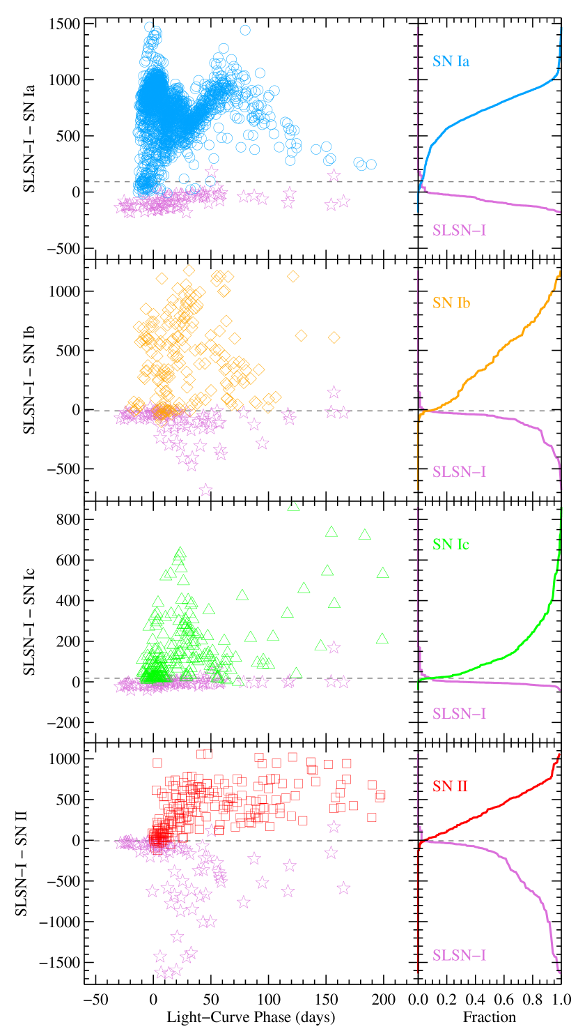
Figure 4: Similar to Figure 3 but for SLSNe-I compared to other types of SNe.

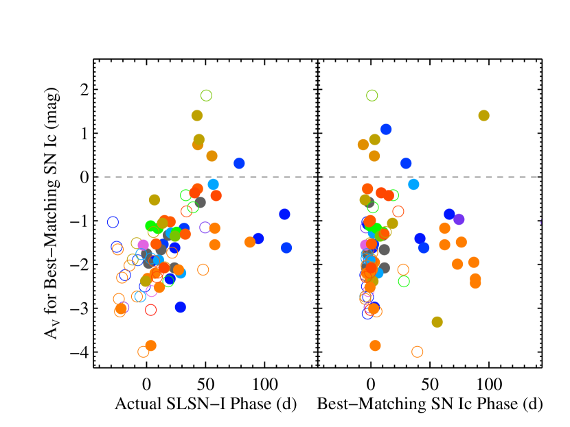
Figure 5: Average $A_{V}$ values found by superfit for the top three SN Ic templates that best match SLSNe-I as a function of the actual light-curve phase (left panel) and the light-curve phase of the best-matching SN Ic template (right panel). Filled circles mark points where the best-matching SN Ic templates are among the top 10 matches returned by superfit on average; open circles mark spectra that were less well fit by SN Ic templates. The symbols are color coded by object as in other figures.

Of all the normal-luminosity SN types, SNe Ic provide the best matches to SLSN-I spectra. However, there is a qualitative difference in these spectra: SLSNe-I typically have much bluer continuum slopes. This can be quantified using the $A_{V}$ parameter output by superfit. In Figure 5 we show the best-fit $A_{V}$ values for the best-matching SN Ic templates. For the continuum slope, the SN Ic templates must be corrected by $A_{V}\approx-2$ mag to match SLSNe-I out to about 1 month past maximum light. After SLSNe-I have evolved 1–2 months past maximum light the mean $A_{V}$ values approach zero, although there is considerable scatter.

Based on the spectral template matching, we also find that SLSNe-I are more likely related to SNe Ic-bl than to ordinary SNe Ic (see also Liu et al. 2016). Given only the choice of SN Ic or SN Ic-bl templates — that is, judging only by the $\Delta I_{\rm SNIc-SNIc-bl}$ scores — we find that 10 of the 15 SLSNe-I in our reference sample are better sorted into the SN Ic-bl group by the method described above.

3 Observations

Now that we have a method to classify objects as SLSNe-I based only on spectra, we turn to the full sample of SN spectra gathered by the Palomar Transient Factory. We will use the techniques described in §2 to identify which PTF objects are spectroscopically similar to SLSNe-I.

3.1 PTF Survey and Follow-Up Observations

The Palomar Transient Factory is a wide-field photometric survey for time-variable objects (Rau et al., 2009; Law et al., 2009). Objects were detected using the 1.2 m Oschin Schmidt Telescope at Palomar Observatory from early 2009 through 2012 (the survey was extended into 2017 as the Intermediate Palomar Transient Factory to bridge the time gap before the Zwicky Transient Facility). A reengineered version of the CFHT-12k camera (renamed the PTF camera) surveyed 7.2 square degrees of sky at $1^{\prime\prime}$ pixel^-1 sampling per exposure. In 60 s, typical SDSS-$g$ and Mould-$R$ limits were 21 mag and 20.5 mag, respectively. The result of the large field-of-view and depth of the PTF survey, combined with over a thousand nights of observations, was the discovery of tens of thousands of candidate transient sources (time-variable, astrophysical sources that are not associated with point sources brighter than the survey limit).

To help assess and classify these candidates, the PTF survey was coupled with an ambitious follow-up program. The neighboring Palomar 1.5 m telescope was used for photometric monitoring of transient sources. Decoupled from the main survey, the Palomar 1.5 m was able to reach greater depths, employ more filters, and target objects at times when the 1.2 m Oschin was surveying other fields. Several nights a month were also reserved for spectroscopic classification of candidates with the Palomar 5.1 m Hale telescope and the twin Keck 10 m telescopes. Additional photometric and spectroscopic follow-up observations were undertaken with a variety of telescopes including the twin Gemini 8 m telescopes, the KPNO 4 m Mayall, the WHT 4.2 m, the NOT 2.5 m, and the Lick 3.0 m Shane.

Even with all of these resources, it was impossible to observe every transient source identified by the PTF survey. During the survey, various selection processes were used in order to tailor the survey to specific targets and to maximize the scientific return from the limited follow-up observations. In general, candidate targets were first identified from the positive residuals remaining after a point-spread-function (PSF) matched image template was subtracted from new observations. Initial, automatic filtering reduced this list to candidates that were found in at least two images at the same sky location within the night and that were found to be roughly consistent with the appearance of a point source. The best candidates were then vetted by humans who ultimately judged if the sources were likely to be astrophysical transients. The list of transient candidates was then passed on to the spectroscopic observes who selected targets to observe. There was not a consistent rubric for this selection. For most of the PTF survey preference for spectroscopic observations was given to targets that appeared to be on the rise, but the final selection was up to the observer at the telescope, who could potentially have a bias to a specific type of SN (e.g., some members of the collaboration were interested in observing SNe Ia while others preferred more rare events). The PTF selection function is thus quite complex but is mostly dictated by the apparent brightness of the targets: brighter targets are easier to observe so more of them can be observed on a given night with a given instrument.

After a spectrum of a candidate was obtained, the data were quickly reduced and posted to a central repository, the “PTF Marshal,” where all collaboration members could access the data and provide comments. Typically an initial classification was provided within a day. Further observations could then be requested for interesting objects or those for which the initial classification proved ambiguous. As the spectra were obtained under multiple observing programs on multiple telescopes, there were naturally multiple pipelines used for the final reduction of the data. Some of these final reductions were posted to the Marshal shortly after the data were taken, but often final reductions were not available until an object was selected for publication. See Gal-Yam et al. (2011) for further details on the PTF candidate vetting process.

3.2 Spectral Extraction Procedures

Most of the spectra presented here were extracted using a custom pipeline implemented in IRAF, Python, and IDL. The data were typically processed using calibration frames taken on the same night. The overscan is subtracted from each raw image and the data are trimmed down to the active window size. The images are then divided by uniformly illuminated exposures (flat fields) obtained from either internal lamps or illuminated dome screens. Next, the background sky including emission lines is fitted and removed from the corrected two-dimensional (2-D) frames using the IDL routine bspline_iterfit.pro following the procedure described by Kelson (2003). The 1-D spectra are then extracted in the optimal manner. An initial wavelength solution is found using calibration-lamp observations. This solution is adjusted based on night-sky lines to account for flexure (the best fit 1-D sky model above is extracted and propagated with the target spectra for this purpose). Observations of standard stars are used to determine the total system throughput as a function of wavelength, and this is used to produce final, flux-calibrated spectra. Observations with Keck/LRIS employed the Atmospheric Dispersion Corrector; observations with other instruments were typically obtained with the slit rotated to the parallactic angle to minimize differential slit losses (Filippenko, 1982). This pipeline was used to extract 1-D spectra from the Keck/LRIS and P200/DBSP observations obtained under Caltech time. The reduction of other datasets was typically done through a similar processes.

We also obtained UV spectra of select events with the Hubble Space Telescope (HST). These data were taken as part of the programs GO-12223 and GO-12524. STIS/MAMA observations from GO-12223 were extracted using the usual Space Telescope Science Institute (STScI) procedures. WFC3 UV grism observations from GO-12524 were extracted using the aXe package from STScI. For these extractions we use LACOSMIC to identify cosmic rays in individual exposures and then stack the data with these pixels masked to produce clean images. Source positions were identified using SExtractor on F200LP and F300X exposures and then input into axecore for extraction. We retain only the dominant spectral order for our analysis.

3.3 Spectroscopic Selection of PTF SLSNe-I

During the survey, several SLSNe-I were identified and monitored. These include some of the first objects to define the SLSN-I class (e.g., Quimby et al. 2011). However, considering our limited understanding of SLSNe-I in the early days of the survey, there is no guarantee that all SLSNe-I were correctly identified in time to obtain further follow-up observations.

With the spectroscopic classification scheme described in §2, we can now search through the spectra in the PTF Marshal to provide a consistent classification of SNe discovered (or identified) by the survey. We begin with the 3432 spectra of 1815 objects in the PTF sample (2009–2012) that were initially classified as SNe and for which redshift estimates are available. For each spectrum we use the superfit output and the cutoff scores from our libraries to determine a classification. We first assess if the spectrum is more like a SN Ia or a SN Ib. We then determine if the spectrum is more like whichever of these provides a better match or a SN Ic. We repeat this process for SNe II, SNe IIb, SNe IIn, and finally SLSNe-I (as noted above, our libraries contain too few SLSNe-II for definitive comparison).

Through this process, we initially identify 100 possible SLSNe-I in the PTF spectral archive. However, we can expect that many of these are simply SNe Ia (and SNe Ia-SS in particular) observed near maximum light. As noted in §2, our simple, phase-independent cut allows a fraction of SNe Ia (especially SNe Ia-SS) to spill into the SLSN-I category. Given the 1783 SN Ia spectra in the PTF archive and a contamination rate of 2.3%, we would expect around 42 SNe Ia to falsely be classified as SLSNe-I with our scheme (note that many of the SNe Ia in our template library were selected by targeted surveys and the sample may therefore have a biased distribution of SN Ia subtypes when compared to the PTF sample; the PTF sample likely contains a higher fraction of SNe Ia-SS). Because the distributions of S/N ratios and host-galaxy contamination factors likely differ from those of the training set, which is preferentially populated with well-observed events, some additional contamination is possible in our first selection of SLSNe-I.

To remove contaminants from the SLSN-I spectroscopic sample, we performed several additional checks. Many of the objects in the initial list had two or more spectra available. In cases where the individual spectra favor different classifications, we gave weight to observations of higher quality. Many objects in the initial list had at least one spectrum with very low S/N ratio that resulted in ambiguous classifications. As these were often reobserved under better conditions or with longer exposure times, the later spectra could be used to more reliably set the classification. We further removed objects that had $\Delta I$ scores only marginally more consistent with SLSNe-I than another type and which showed the characteristic spectral features of the other type. For example, objects that showed a clear Si II $\lambda$6150 feature were reclassified as SNe Ia. We removed all such marginal SLSN-I candidates that had SN Ia (and not SN Ic or SN Ib) as the second-best classification.

After careful consideration of the initial 100 possible SLSNe-I, we find that 19 of these objects are spectroscopically consistent with SLSNe-I while another 4 objects are possibly consistent but a definitive statement cannot be made. In Table 3 we list these objects and label them as “SLSN-I” and “possible SLSN-I” candidates, respectively. The remaining SLSN-I candidates are mostly SNe Ia that passed the automatic cut as described above, but we also removed several objects with poor-quality spectra. Note that to this point we have made no conscious use of the photometry or host-galaxy properties in identifying our sample; we have simply constructed a sample of objects that have spectra that are more consistent with SLSNe-I than with any other type.

The SLSN-I reference sample does, however, contain several PTF objects (PTF09atu, PTF09cnd, PTF09cwl, SN 2010gx, PTF10hgi, SN 2011ke, PTF11rks, and PTF12dam). As noted above, we always exclude any spectral matches to templates in our libraries that belong to the object being classified, but nonetheless the knowledge that these objects have previously been classified as SLSNe-I could bias our vetting process. For the 11 new SLSNe-I in the spectroscopic sample, we did not knowingly use any information other than the spectra for the final classification, but it should be noted that some of these objects had also been initially classified as SLSNe-I, and their light curve and host-galaxy properties were not formally blinded during the final vetting process. It should also be noted that there are additional objects in the PTF archive that have spectra but which were not classified as SNe or for which redshifts have not been determined. These spectra are typically of inferior quality and it is uncertain if they alone can provide useful constraints on the classification (e.g., the initial quick-look analysis failed to yield a classification). There may further be human errors, such as spectra assigned to the wrong object, that can disrupt the classification process (e.g., see PTF10gvb below).

3.4 PTF SLSN-I Sample

Below we give the details for the 19 SLSN-I and 4 possible SLSN-I spectroscopic samples. Unless otherwise specified, host-galaxy information is taken from Perley et al. (2016) and light-curve peak dates and absolute magnitudes are adopted from De Cia et al. (2017). Spectral observations are listed in Table LABEL:table:speclog and shown in Figures 28–38 in the Appendix.

Table 3: PTF Spectroscopic SLSN-I Sample

Name	$\alpha$(J2000)	$\delta$(J2000)	$z$	MJDpeak	$M_{\rm peak}$	$N_{\rm spec}$	Spec. Class
PTF09as	12:59:15.78	$+$27:16:38.5	0.1864	54918.2	$\cdots$	1	SLSN-I
PTF09atu	16:30:24.55	$+$23:38:25.0	0.5014	55062.3	$-21.75$	7	SLSN-I
PTF09cnd	16:12:08.94	$+$51:29:16.2	0.2585	55085.3	$-22.18$	13	SLSN-I
PTF09cwl	14:49:10.08	$+$29:25:11.4	0.3502	55067.2	$-21.92$	6	SLSN-I
PTF10bfz	12:54:41.27	$+$15:24:17.0	0.1699	55227.5	$-21.06$	5	SLSN-I
PTF10bjp	10:06:34.30	$+$67:59:19.0	0.3585	55251.5	$-20.54$	2	SLSN-I
SN 2010gx (PTF10cwr)	11:25:46.67	$-$08:49:41.2	0.2301	55281.2	$-21.62$	5	SLSN-I
PTF10hgi	16:37:47.04	$+$06:12:32.3	0.0982	55367.4	$-20.35$	13	SLSN-Ia
PTF10nmn	15:50:02.79	$-$07:24:42.1	0.1236	55384.2	$-20.53$	9	SLSN-I
PTF10uhf	16:52:46.68	$+$47:36:22.0	0.2879	55452.3	$-20.68$	3	SLSN-I
PTF10vqv	03:03:06.84	$-$01:32:34.9	0.4520	55470.5	$-21.55$	7	SLSN-I
SN 2010hy (PTF10vwg)	18:59:32.86	$+$19:24:25.7	0.19	55457.3	$-22.09$	2	SLSN-I
PTF10aagc	09:39:56.93	$+$21:43:16.9	0.2067	55499.5	$-20.25$	8	SLSN-I
SN 2011ke (PTF11dij)	13:50:57.77	$+$26:16:42.8	0.1429	55683.4	$-21.39$	9	SLSN-I
PTF11hrq	00:51:47.22	$-$26:25:10.0	0.0571	55753.5	$-20.05$	4	SLSN-I
PTF11rks	01:39:45.51	$+$29:55:27.0	0.1924	55936.1	$-20.92$	7	SLSN-I
PTF12dam	14:24:46.20	$+$46:13:48.3	0.1075	56093.3	$-21.69$	15	SLSN-I
PTF12gty	16:01:15.23	$+$21:23:17.4	0.1768	56143.4	$-20.04$	2	SLSN-I
PTF12mxx	22:30:16.68	$+$27:58:21.9	0.3274	56290.1	$-21.61$	2	SLSN-I
PTF09q	12:24:50.11	$+$08:25:58.8	0.09	54910.0	$\cdots$	1	possible SLSN-I
PTF10gvb	12:15:32.28	$+$40:18:09.5	0.098	55337.2	$-19.58$	3	possible SLSN-I
PTF11mnb	00:34:13.25	$+$02:48:31.4	0.0603	55855.3	$-18.91$	5	possible SLSN-I
PTF12hni	22:31:55.86	$-$06:47:49.0	0.1056	56155.3	$-19.96$	3	possible SLSN-I

^aSpectra of PTF10hgi show clear evidence for hydrogen and helium. Based on this it may better be classified as a SLSN-IIb.

PTF09q was found at the beginning of the PTF survey while the system was still being commissioned. It was actually discovered before the PTF naming convention had been settled, so it was first announced as PTF-OT4 (Kasliwal et al., 2009a) and later given the IAU name SN 2009bh (Kasliwal et al., 2009b); for convenience we adopt the final PTF name (PTF09q) in this work. The object was initially classified as a SN Ic. In our reanalysis of this classification, we find that SN Ic templates, such as SN 2005az at $t=-6$ d, do provide reasonable matches to the single spectrum obtained, but SLSNe-I, such as SN 2011ke at $t=+24$ d, are possible matches as well (template phases are taken from the original source; most SNe Ia, SNe Ic, and SLSNe-I phases are relative to $B$-band, $V$-band, and SDSS-$g$ maximum light, respectively). We thus place PTF09q in the possible SLSN-I sample. The object appears to be hosted by a massive galaxy, which would be unusual for a SLSN-I (e.g., Perley et al. 2016), but there are exceptions to this (e.g., Nicholl et al. 2017a; Bose et al. 2017), and the host galaxy could be star-forming. The photometric peak of PTF09q is well below the standard $M<-21$ mag traditionally required of SLSNe (Gal-Yam, 2012).

PTF09as was identified by the PTF survey on 2009 March 27 (UT dates are used throughout this paper) and a single spectrum was obtained on 2009 March 31. A transient source matching the location of this object was independently reported by CRTS as CSS090319:125916+271641 (Drake et al., 2009a) and was later given the IAU name SN 2009cb (Drake et al., 2009b). The source was actually first classified as a SN Ia by PTF (Quimby et al., 2009a, b), but our reanalysis casts doubt on this initial classification. With the large libraries of SN templates now available, we find that the spectrum of PTF09as is far better matched to SLSN-I templates, such as SN 2011ke at $t=+53$ d. The SN is apparently hosted by a dwarf galaxy.

PTF09atu, PTF09cwl (= SN 2009jh), and PTF09cnd have previously been published as SLSNe-I (Quimby et al., 2011). We confirm that the spectra of these objects are better matches to other SLSNe-I than to any other SN type, and we present multiple new spectroscopic observations of each target here for the first time. We also provide significantly improved extractions of the previously published spectra for these objects (and for SN 2010gx below).

PTF10bfz was identified by PTF as an optical transient on 2010 Feb. 1, but its spectral classification was not immediately obvious. Later that year after several spectra had been taken it was concluded to be a SN Ic-BL event (Arcavi et al., 2010). However, our reanalysis strongly favors classification as a SLSN-I. The fourth spectrum in particular is best matched to SLSN-I templates including PTF11rks at $t=+7$ d. This classification is supported by an apparent dwarf host galaxy and a peak brighter than $-21$ mag.

PTF10bjp was identified as a transient candidate on 2010 Feb. 21. Two spectra were obtained that, although relatively noisy, showed broad features consistent with those of SNe and of SLSNe-I in particular. Our reanalysis confirms this source to be a SLSN-I. The first spectrum is well matched by PTF12dam at $t=+49$ d. The apparent host galaxy is a dwarf. The peak absolute magnitude recorded is $-20.5$, which would be below the traditional cutoff for SLSNe.

SN 2010gx (= PTF10cwr) and PTF10hgi have previously been published as SLSNe-I (e.g., Pastorello et al. 2010; Quimby et al. 2011; Inserra et al. 2013; Chen et al. 2013). We confirm that these sources have spectra that are best matched by SLSN-I templates through our automated process. However, PTF10hgi is peculiar in the sense that it has obvious hydrogen Balmer and He I lines in contrast to other SLSNe-I, and thus it may be better classified as a SLSN-IIb. We discuss this further in §6.6.

PTF10gvb was first identified as a possible SN on 2010 May 6, and it was spectroscopically vetted with LRIS on Keck-I later that same night. This first spectrum is mostly featureless except for two broad dips around 5400 Å and 6100 Å in the host-galaxy rest frame. This spectrum is roughly similar to early-phase spectra of PTF09cnd and PTF12dam, but the PTF10gvb spectra lack the characteristic O II features around 4200 to 4500 Å. A second spectrum taken on 2010 May 15 is well matched by the peculiar SN Ib SN 2009er near maximum light and also to various SNe Ic-bl. A final spectrum taken on 2010 is similar to the SN Ic-bl SN 2003jd around three weeks after maximum light (including data outside the 3900–7000 Å range, the phase of the best matches increases to roughly $+50$ days). Based on this final spectrum it was internally classified as a SN Ic-bl. However, the first two spectra are roughly consistent with a SLSN-I, so we consider this object a possible SLSN-I. We note that when we first applied our spectroscopic selection process described above, this object was not identified as a possible SLSN-I because spectra of another object had been mistakenly included. The bolometric light curve of PTF10gvb was studied by Prentice et al. (2016). The host galaxy is blue, of intermediate mass, and star-forming (Taggart et al., in prep.).

PTF10nmn has been presented by Gal-Yam (2012) and will be further discussed by Yaron et al. (in prep.). We confirm that this object is most spectroscopically similar to SLSNe-I (we do not use the SLSN-R classification in this work). In particular, the first spectra are similar to those of PTF12dam at 2–3 months after maximum brightness.

PTF10uhf first showed a mostly featureless spectrum on 2010 Sep. 8, which was two days after the target was first identified by PTF. Later spectra exhibit several SN-like features, and we find a reasonable match to SN 2011ke at $t=+26$ d for the second spectrum. As noted by Perley et al. (2016), the apparent host galaxy of this target is atypically luminous for a SLSN-I. PTF10uhf reached an absolute magnitude of $-20.7$, which is below the traditional SLSN threshold but which would be extremely luminous for a typical SN Ic.

PTF10vqv was announced as a possible SLSN-I similar to PTF09cnd by Quimby et al. (2010). Seven spectra were obtained, although most have relatively low S/N ratios. We can confirm, however, that the spectra are best matched by SLSN-I templates if the lowest-quality spectra are ignored. The second spectrum, which is of reasonable quality, is well matched to PTF09cnd at $t=+28$ d. The peak absolute magnitude of PTF10vqv ($-21.6$) and the faintness of the host galaxy are also consistent with typical SLSNe-I.

SN 2010hy was not discovered by PTF; rather, it was recovered in PTF survey data after it was first announced by the Lick Observatory Supernova Search (LOSS; Filippenko et al., 2001) with the Katzman Automatic Imaging Telescope (KAIT; Kodros et al., 2010), who noted that the target appeared to be a high-luminosity SN Ic, although they could not rule out a SN Ia classification. Owing to the low Galactic latitude ($b\approx 7^{\circ}$), the field was not searched promptly as was typically the case in PTF. Nonetheless, we report here on our spectroscopic follow-up observations of SN 2010hy, which also has the PTF identifier PTF10vwg. The spectra are heavily reddened by dust in the Galaxy, though the spectral features are consistent with those of SLSNe-I. Our data strongly suggest the source is not a SN Ia, but the contrast with SNe Ic is weaker. The first spectrum is similar to that of SSS120810 at $t=+59$ d. Both of our spectra favor SLSN-I more than any other type, yet the index difference, $\Delta I_{\rm SLSN-I-Ic}$, is positive and only just below the cutoff threshold. But both spectra are below the threshold, so we place this object in the SLSN-I sample. After correcting for Galactic extinction, the peak absolute magnitude is about $-22$ mag, which is well above the SLSN threshold. The host galaxy is also apparently faint and thus similar to other SLSN-I hosts.

PTF10aagc was flagged as a transient event on 2010 Nov. 3. From the first spectra, obtained the following night, the target was identified as a possible SLSN-I. The early-time spectra are similar to those of SN 2010gx at $t=+5$ d. The SN is offset from a dwarf galaxy. The peak absolute magnitude, $-20.3$, would be high for a SN Ic but is below the traditional dividing line for SLSNe. As we discuss further in §6.6, PTF10aagc also shows hydrogen features in its spectra, but the spectra qualitatively differ from those of published SLSNe-II, so we choose to keep it in the SLSN-I sample. PTF10aagc was also discussed by Yan et al. (2015).

SN 2011ke (= PTF11dij), PTF11rks, and PTF12dam have all previously been published as SLSNe-I (e.g., Inserra et al. 2013; Nicholl et al. 2013; Vreeswijk et al. 2017). We confirm that these objects have spectra more similar to those of SLSNe-I than to any other SN type.

PTF11hrq was originally identified as a possible variable-star candidate owing to its compact host galaxy (e.g., Cikota et al. 2017). It was eventually identified as a potential SN based on its slowly declining light curve. This prompted spectroscopic follow-up observations about one year after the first identification of the source that led to classification as a SLSN-I similar to PTF10nmn above (as was anticipated from the light-curve behavior).

PTF11mnb was identified by the PTF survey on 2011 Sep. 19. It was noted to have an unusually slow rise to maximum, its first spectrum was initially suggested to show some similarities to those of SN 1999as (e.g., Hatano et al. 2001), and it was internally categorized as a likely SN Ic. The first spectrum is noisy, but a second spectrum taken about two weeks later is a good match to SN 2007gr about 1 week after maximum light. However, this spectrum is also reasonably well matched to SLSNe-I at later light-curve phases, such as SN 2012il at $t=+55$ d. Given the good matches to SNe Ic and the possible matches to SLSNe-I, we place this object in our possible SLSN-I sample. PTF11mnb reached a peak absolute magnitude of about $-18.9$, and its apparent host galaxy is a dwarf ($M_{g}\approx-18$ mag based on SDSS photometry). This object is further discussed in a separate paper (Taddia et al., in prep.).

PTF12hni was identified by PTF on 2012 Aug. 8, which was likely near or after the photometric maximum. The classification of the spectrum was initially ambiguous, with possible matches to both SNe Ia and SNe Ic found, but the redshift favored by template matching suggested that this was a relatively distant and thus luminous source. In our analysis, the first spectrum is reasonably well matched by the SN Ic 2007gr at $t=-1$ d. It may also match SN 2003jd at $\sim 3$ weeks past photometric maximum, but to do this superfit requires a significantly negative $A_{V}$ (e.g., the templates must be made bluer to match the data). We also find plausible matches to SLSNe-I at even later phases, such as PTF09atu at $t=+98$ d. For the second spectrum, superfit prefers matches to PTF12dam at 2–3 months after photometric maximum, but the SN Ia-SS (a SN 2002cx-like event) SN 2008A at $t=+43$ d also provides a good match. We thus consider PTF12hni a plausible member of the SLSN-I spectroscopic class and place it in the possible SLSN-I sample. The target was observed to be as bright as $-20$ mag absolute, but, again, it was likely caught after maximum. The SN is located on the sky in between two galaxies at different redshifts: a large, blue galaxy at $z=0.106$ and a smaller, redder galaxy at $z=0.185$. Both galaxies are strongly star-forming, but only the lower-redshift and larger galaxy is at a redshift consistent with that measured from the SN features. Its properties are consistent with an intermediate-mass and relatively metal-poor galaxy undergoing rapid star formation (Taggart et al., in prep.).

PTF12gty was first identified as a variable-star candidate on 2012 July 18, but soon thereafter it was realized that the recently updated reference image had been constructed with images including light from PTF12gty. The target was upgraded to a SN candidate and a spectrum taken the following week was found to be consistent with a SLSN-I. In particular, we find matches to PTF12dam at about 2–3 months after maximum light. The transient is well offset from a large elliptical galaxy, but the SDSS redshift of this object, $z=0.031$, indicates that it is an unrelated foreground galaxy. A weak (uncataloged) source is present near the SN position in PS1 images, indicating the true host must be very faint. The detection of clear H II-region lines in our late-time SN spectra indicates a fairly high star-formation rate (Taggart et al., in prep.). The peak absolute magnitude of PTF12gty is only $-20.0$.

PTF12mxx was found near the end of the original PTF survey on 2012 Dec. 15. The target was identified as a SLSN-I through spectroscopy obtained three nights later. The spectra are well matched by PTF12dam at $t=-21$ d. The high peak luminosity and faint host galaxy are further similar to typical SLSN-I hosts.

Table 4: Log of Spectroscopic Observations

Name	Date	LC Phase	Inst.	Range	Spec. Phase	Spec. Phase
	(UT)	(days)		(Å)	(fiducial)	(fit)
PTF09q	2009-03-20	$-0.0$	Palomar-5m/DBSP	$3016-10204$	$\cdots$	$1.27\pm 0.22$
PTF09as	2009-03-31	$+2.4$	Keck-I/LRIS	$3026-9316$	$\cdots$	$1.35\pm 0.09$
PTF09atu	2009-07-20	$-20.2$	Keck-I/LRIS	$3001-10297$	$-0.68$	$-0.58\pm 0.25$
PTF09atu	2009-07-22	$-18.9$	Keck-I/LRIS	$3001-10285$	$-0.61$	$-0.58\pm 0.25$
PTF09atu	2009-08-25	$+3.8$	Keck-I/LRIS	$3005-10296$	$0.25$	$0.20\pm 0.09$
PTF09atu	2009-09-23	$+23.1$	Keck-I/LRIS	$3001-10296$	$1.00$	$1.21\pm 0.38$
PTF09atu	2009-10-16	$+38.4$	Keck-I/LRIS	$3106-8811$	$1.61$	$1.43\pm 0.26$
PTF09atu	2010-01-14	$+98.4$	Keck-I/LRIS	$3001-10296$	$\cdots$	$1.40\pm 0.16$
PTF09atu	2010-02-11	$+117.0$	Keck-I/LRIS	$3001-10264$	$1.73$	$1.77\pm 0.08$
PTF09cwl	2009-08-25	$+0.6$	Keck-I/LRIS	$3005-10296$	$-0.46$	$-0.49\pm 0.13$
PTF09cwl	2009-09-23	$+22.0$	Keck-I/LRIS	$3001-10296$	$0.54$	$0.78\pm 0.27$
PTF09cwl	2009-10-17	$+39.8$	Keck-I/LRIS	$3105-8796$	$1.48$	$1.35\pm 0.23$
PTF09cwl	2009-12-19	$+86.5$	Keck-I/LRIS	$3001-10296$	$1.83$	$1.65\pm 0.32$
PTF09cwl	2010-02-11	$+126.5$	Keck-I/LRIS	$3001-10265$	$\cdots$	$1.72\pm 0.36$
PTF09cwl	2011-06-02	$+479.0$	Keck-I/LRIS	$3001-10297$	$\cdots$	$1.37\pm 0.14$
PTF09cnd	2009-08-12	$-24.1$	WHT/ISIS	$3261-8159$	$-1.00$	$-0.66\pm 0.25$
PTF09cnd	2009-08-16	$-20.9$	Palomar-5m/DBSP	$3001-10237$	$-0.96$	$-0.66\pm 0.23$
PTF09cnd	2009-08-25	$-13.8$	Keck-I/LRIS	$3005-10297$	$-0.64$	$-0.56\pm 0.08$
PTF09cnd	2009-09-15	$+2.9$	WHT/ISIS	$3151-8179$	$-0.38$	$-0.50\pm 0.14$
PTF09cnd	2009-09-23	$+9.3$	Keck-I/LRIS	$3001-10296$	$-0.33$	$-0.36\pm 0.23$
PTF09cnd	2009-10-12	$+24.4$	WHT/ISIS	$3151-8163$	$0.37$	$0.50\pm 0.15$
PTF09cnd	2009-10-17	$+28.3$	Keck-I/LRIS	$3105-8809$	$0.51$	$0.92\pm 0.49$
PTF09cnd	2009-10-23	$+33.1$	Keck-I/LRIS	$3481-10195$	$0.57$	$0.99\pm 0.46$
PTF09cnd	2010-01-14	$+99.0$	Keck-I/LRIS	$3001-10297$	$1.77$	$1.64\pm 0.31$
PTF09cnd	2010-02-11	$+121.3$	Keck-I/LRIS	$3001-10263$	$1.88$	$1.85\pm 0.07$
PTF09cnd	2010-07-09	$+238.9$	Keck-I/LRIS	$3117-10230$	$\cdots$	$1.97\pm 0.08$
PTF09cnd	2010-09-05	$+285.0$	Keck-I/LRIS	$3003-10228$	$\cdots$	$1.57\pm 0.68$
PTF09cnd	2011-07-02	$+523.4$	Keck-I/LRIS	$3001-10074$	$\cdots$	$1.12\pm 1.05$
PTF10bfz	2010-02-07	$+5.6$	Keck-I/LRIS	$3499-9998$	$-0.13$	$0.38\pm 0.72$
PTF10bfz	2010-02-11	$+9.0$	Keck-I/LRIS	$3001-10262$	$0.17$	$0.86\pm 0.62$
PTF10bfz	2010-02-21	$+17.6$	WHT/ISIS	$3149-9499$	$1.17$	$1.33\pm 0.07$
PTF10bfz	2010-03-07	$+29.5$	Keck-I/LRIS	$3001-9582$	$1.23$	$1.33\pm 0.08$
PTF10bfz	2013-05-10	$+1021.1$	Keck-I/LRIS	$3149-10274$	$\cdots$	$1.21\pm 0.46$
PTF10bjp	2010-03-07	$+7.7$	Keck-I/LRIS	$3001-10272$	$1.09$	$1.51\pm 0.54$
PTF10bjp	2010-03-14	$+12.9$	Keck-I/LRIS	$3253-7602$	$\cdots$	$1.28\pm 0.62$
SN 2010gx	2010-03-18	$-6.7$	Palomar-5m/DBSP	$3007-9298$	$-1.04$	$-0.79\pm 0.21$
SN 2010gx	2010-04-08	$+10.4$	Palomar-5m/DBSP	$3003-9299$	$0.39$	$0.79\pm 0.35$
SN 2010gx	2010-05-07	$+34.0$	Palomar-5m/DBSP	$3029-9299$	$1.58$	$1.44\pm 0.10$
SN 2010gx	2010-06-17	$+67.3$	Keck-I/LRIS	$3053-10296$	$\cdots$	$1.64\pm 0.20$
SN 2010gx	2011-03-26	$+296.5$	Keck-I/LRIS	$3012-10260$	$\cdots$	$1.03\pm 0.50$
PTF10hgi	2010-05-21	$-27.7$	Palomar-5m/DBSP	$3001-10288$	$-0.09$	$0.26\pm 0.72$
PTF10hgi	2010-06-11	$-8.6$	Lick-3m/Kast	$3443-10157$	$-0.07$	$-0.12\pm 0.32$
PTF10hgi	2010-07-07	$+15.1$	Lick-3m/Kast	$3429-10163$	$0.45$	$0.62\pm 0.27$
PTF10hgi	2010-07-08	$+16.0$	Keck-I/LRIS	$3499-9999$	$0.48$	$0.62\pm 0.27$
PTF10hgi	2010-07-14	$+21.5$	Palomar-5m/DBSP	$3549-9899$	$1.02$	$0.90\pm 0.51$
PTF10hgi	2010-07-19	$+26.0$	Lick-3m/Kast	$3477-9929$	$1.11$	$1.09\pm 0.55$
PTF10hgi	2010-08-11	$+47.0$	Keck-I/LRIS	$3004-10236$	$1.66$	$1.59\pm 0.15$
PTF10hgi	2010-09-05	$+69.7$	Palomar-5m/DBSP	$3439-9849$	$1.82$	$1.71\pm 0.14$
PTF10hgi	2010-09-10	$+74.3$	KPNO-4m/RCspec	$3319-8397$	$1.84$	$1.75\pm 0.14$
PTF10hgi	2010-10-03	$+95.2$	Keck-I/LRIS	$3001-10297$	$1.87$	$1.76\pm 0.13$
PTF10hgi	2010-11-01	$+121.6$	Keck-I/LRIS	$3218-7591$	$1.93$	$1.92\pm 0.07$
PTF10hgi	2011-03-12	$+240.9$	Keck-I/LRIS	$3001-10297$	$1.94$	$1.93\pm 0.04$
PTF10hgi	2011-06-01	$+314.7$	Keck-II/DEIMOS	$4652-9625$	$2.06$	$1.97\pm 0.05$
PTF10gvb	2010-05-06	$-13.8$	Keck-I/LRIS	$3500-10000$	$\cdots$	$-0.17\pm 0.13$
PTF10gvb	2010-05-15	$-5.6$	Keck-I/LRIS	$3300-10180$	$\cdots$	$1.12\pm 0.52$
PTF10gvb	2010-07-08	$+43.6$	Keck-I/LRIS	$3120-10040$	$\cdots$	$1.39\pm 0.59$
PTF10nmn	2010-07-07	$-0.2$	Keck-I/LRIS	$3299-10200$	$1.75$	$1.80\pm 0.09$
PTF10nmn	2010-07-14	$+6.1$	Palomar-5m/DBSP	$3200-9461$	$1.76$	$1.33\pm 0.24$
PTF10nmn	2010-07-15	$+6.9$	Palomar-5m/DBSP	$3480-10000$	$1.78$	$1.78\pm 0.07$
PTF10nmn	2010-08-09	$+29.2$	Palomar-5m/DBSP	$3001-10044$	$1.86$	$1.83\pm 0.06$
PTF10nmn	2011-01-28	$+182.3$	Palomar-5m/DBSP	$3490-9750$	$1.95$	$1.94\pm 0.04$
PTF10nmn	2011-03-04	$+213.4$	Keck-I/LRIS	$3011-10297$	$1.96$	$1.90\pm 0.06$
PTF10nmn	2011-06-01	$+292.6$	Keck-II/DEIMOS	$4652-9626$	$\cdots$	$1.38\pm 1.42$
PTF10nmn	2011-07-03	$+321.1$	Keck-I/LRIS	$3001-10297$	$2.01$	$2.00\pm 0.06$
PTF10nmn	2012-02-20	$+527.6$	Keck-I/LRIS	$3081-10271$	$2.02$	$1.57\pm 1.01$
PTF10uhf	2010-09-08	$-4.1$	KPNO-4m/RCspec	$3499-8435$	$1.13$	$0.98\pm 0.52$
PTF10uhf	2010-10-03	$+15.3$	Keck-I/LRIS	$3001-10292$	$1.15$	$1.36\pm 0.08$
PTF10uhf	2011-07-02	$+226.5$	Keck-I/LRIS	$3001-10076$	$\cdots$	$1.38\pm 0.03$
SN 2010hy	2010-10-14	$+21.6$	Keck-I/LRIS	$3105-10239$	$1.43$	$1.44\pm 0.16$
SN 2010hy	2011-03-12	$+146.8$	Keck-I/LRIS	$3001-10296$	$1.89$	$1.84\pm 0.08$
PTF10vqv	2010-10-11	$+6.5$	KPNO-4m/RCspec	$3840-8400$	$-0.04$	$0.88\pm 0.88$
PTF10vqv	2010-10-17	$+10.7$	Palomar-5m/DBSP	$3001-9966$	$0.28$	$0.47\pm 0.10$
PTF10vqv	2010-11-01	$+21.0$	Keck-I/LRIS	$3219-7591$	$1.53$	$1.33\pm 0.76$
PTF10vqv	2010-12-06	$+45.1$	Palomar-5m/DBSP	$3500-10000$	$\cdots$	$1.04\pm 0.72$
PTF10vqv	2010-12-08	$+46.5$	Keck-I/LRIS	$3299-10000$	$1.55$	$1.40\pm 0.19$
PTF10vqv	2011-01-31	$+83.7$	Keck-I/LRIS	$3001-10252$	$\cdots$	$0.60\pm 0.27$
PTF10vqv	2011-02-01	$+84.4$	Keck-I/LRIS	$3004-10248$	$\cdots$	$1.58\pm 0.28$
PTF10aagc	2010-11-04	$+3.7$	KPNO-4m/RCspec	$3329-8459$	$-0.25$	$-0.17\pm 0.15$
PTF10aagc	2010-11-05	$+4.6$	Keck-I/LRIS	$3299-7633$	$-0.23$	$-0.56\pm 0.22$
PTF10aagc	2010-11-07	$+6.2$	Keck-II/DEIMOS	$4480-9631$	$-0.20$	$0.04\pm 0.64$
PTF10aagc	2010-11-18	$+15.3$	TNG/DOLORES	$3303-8097$	$1.51$	$1.41\pm 0.06$
PTF10aagc	2010-11-30	$+25.3$	Palomar-5m/DBSP	$3001-9299$	$\cdots$	$1.60\pm 0.23$
PTF10aagc	2010-12-08	$+31.9$	Keck-I/LRIS	$3299-10000$	$1.52$	$0.99\pm 0.54$
PTF10aagc	2011-02-01	$+77.5$	Keck-I/LRIS	$3004-10244$	$1.56$	$1.55\pm 0.07$
PTF10aagc	2011-03-26	$+121.4$	Keck-I/LRIS	$3013-10256$	$\cdots$	$1.45\pm 0.13$
SN 2011ke	2011-05-11	$+7.6$	KPNO-4m/RCspec	$3473-8357$	$0.20$	$0.71\pm 0.54$
SN 2011ke	2011-05-13	$+9.3$	KPNO-4m/RCspec	$3449-8450$	$0.23$	$0.71\pm 0.53$
SN 2011ke	2011-05-25	$+19.8$	Palomar-5m/DBSP	$3001-10256$	$1.28$	$1.34\pm 0.11$
SN 2011ke	2011-05-30	$+24.2$	HST/STIS	$1580-3150$	$\cdots$	$-0.09\pm 1.34$
SN 2011ke	2011-06-01	$+25.9$	Keck-II/DEIMOS	$4530-9625$	$1.38$	$1.39\pm 0.06$
SN 2011ke	2011-06-07	$+31.2$	KPNO-4m/RCspec	$3390-8459$	$1.40$	$1.39\pm 0.06$
SN 2011ke	2011-07-02	$+53.0$	Keck-I/LRIS	$3001-10077$	$1.59$	$1.49\pm 0.19$
SN 2011ke	2012-01-26	$+235.0$	Keck-I/LRIS	$3001-10293$	$\cdots$	$-0.56\pm 0.48$
SN 2011ke	2012-03-23	$+284.9$	Keck-I/LRIS	$3181-9325$	$\cdots$	$0.61\pm 0.69$
PTF11mnb	2011-10-07	$-13.4$	UH88/SNIFS	$3301-9701$	$\cdots$	$1.62\pm 0.11$
PTF11mnb	2011-10-30	$+8.3$	Palomar-5m/DBSP	$3001-10293$	$\cdots$	$1.72\pm 0.13$
PTF11mnb	2011-11-26	$+33.7$	Keck-I/LRIS	$3001-10296$	$\cdots$	$1.78\pm 0.11$
PTF11mnb	2011-12-21	$+57.3$	Palomar-5m/DBSP	$3001-10296$	$\cdots$	$1.88\pm 0.08$
PTF11mnb	2012-01-27	$+92.2$	KPNO-4m/RCspec	$3574-8137$	$\cdots$	$1.84\pm 0.14$
PTF11rks	2011-12-27	$-11.9$	Palomar-5m/DBSP	$3175-10296$	$-0.92$	$-0.73\pm 0.32$
PTF11rks	2011-12-31	$-8.5$	Keck-I/LRIS	$3001-10297$	$-0.88$	$-0.60\pm 0.16$
PTF11rks	2012-01-17	$+5.8$	HST/WFC3	$1903-5185$	$\cdots$	$-0.09\pm 1.34$
PTF11rks	2012-01-18	$+6.6$	Palomar-5m/DBSP	$3022-10296$	$0.88$	$1.12\pm 0.25$
PTF11rks	2012-02-01	$+18.3$	Palomar-5m/DBSP	$3001-10295$	$\cdots$	$1.31\pm 0.10$
PTF11rks	2012-03-01	$+42.7$	WHT/ISIS	$5501-9499$	$\cdots$	$1.32\pm 0.09$
PTF11rks	2012-07-15	$+156.7$	Keck-I/LRIS	$3002-9443$	$\cdots$	$0.88\pm 1.05$
PTF11hrq	2011-12-27	$+159.4$	Palomar-5m/DBSP	$3178-10295$	$1.97$	$1.93\pm 0.05$
PTF11hrq	2012-07-15	$+349.6$	Keck-I/LRIS	$3003-9440$	$1.99$	$1.55\pm 0.99$
PTF11hrq	2012-12-09	$+488.6$	Keck-II/DEIMOS	$4907-9300$	$2.03$	$1.45\pm 0.73$
PTF11hrq	2012-12-12	$+491.5$	Keck-I/LRIS	$3002-10264$	$2.04$	$1.54\pm 0.99$
PTF12dam	2012-05-20	$-23.8$	Lick-3m/Kast	$3465-5558$	$-0.58$	$-0.62\pm 0.22$
PTF12dam	2012-05-21	$-22.9$	Lick-3m/Kast	$3447-10239$	$-0.55$	$-0.47\pm 0.22$
PTF12dam	2012-05-22	$-22.0$	Keck-I/LRIS	$3003-10247$	$-0.52$	$-0.54\pm 0.15$
PTF12dam	2012-05-25	$-19.3$	WHT/ISIS	$3500-9498$	$-0.41$	$-0.66\pm 0.27$
PTF12dam	2012-05-26	$-18.4$	HST/WFC3	$1903-5185$	$-0.36$	$-0.74\pm 0.20$
PTF12dam	2012-06-14	$-1.2$	Lick-3m/Kast	$3499-9999$	$-0.02$	$1.71\pm 0.27$
PTF12dam	2012-06-18	$+2.4$	Palomar-5m/DBSP	$3001-10295$	$0.00$	$0.08\pm 0.34$
PTF12dam	2012-07-06	$+18.7$	HST/WFC3	$1903-5198$	$0.60$	$0.62\pm 0.41$
PTF12dam	2012-07-11	$+23.2$	Lick-3m/Kast	$3529-10221$	$0.64$	$0.80\pm 0.52$
PTF12dam	2012-07-12	$+24.1$	HST/WFC3	$1903-5185$	$1.04$	$0.73\pm 0.45$
PTF12dam	2012-08-20	$+59.3$	WHT/ISIS	$3500-9499$	$1.71$	$1.55\pm 0.29$
PTF12dam	2012-12-05	$+155.9$	Palomar-5m/DBSP	$3001-9298$	$1.81$	$1.86\pm 0.08$
PTF12dam	2013-04-09	$+268.8$	Keck-I/LRIS	$3060-10288$	$1.98$	$1.97\pm 0.04$
PTF12dam	2013-06-09	$+323.9$	Keck-I/LRIS	$3002-10266$	$2.05$	$1.98\pm 0.04$
PTF12dam	2014-04-29	$+616.4$	Keck-I/LRIS	$3068-5677$	$\cdots$	$1.16\pm 1.15$
PTF12gty	2012-07-22	$-11.4$	Lick-3m/Kast	$3499-10000$	$1.70$	$1.73\pm 0.05$
PTF12gty	2012-07-27	$-7.1$	Palomar-5m/DBSP	$3002-10295$	$1.72$	$1.61\pm 0.29$
PTF12hni	2012-08-09	$-6.6$	Lick-3m/Kast	$3500-9999$	$\cdots$	$1.52\pm 0.11$
PTF12hni	2012-08-19	$+2.5$	Keck-I/LRIS	$3408-10250$	$\cdots$	$1.63\pm 0.12$
PTF12hni	2013-07-12	$+298.3$	Keck-II/DEIMOS	$4905-10119$	$\cdots$	$1.91\pm 0.23$
PTF12mxx	2012-12-18	$-8.4$	Keck-I/LRIS	$3299-10199$	$-0.71$	$-0.53\pm 0.14$
PTF12mxx	2013-01-08	$+7.4$	Keck-II/DEIMOS	$4499-9635$	$0.14$	$0.22\pm 0.08$

4 SLSN-I Spectral Sequence

Traditionally, a spectrum of a given SN is compared to spectra of other objects of the same class at a similar light-curve phase. For homogeneous object types this works quite successfully. For a given SN Ia spectrum, for example, we find that the best matches in our template library can be used to accurately predict the light-curve phase to a precision of about $\pm 2$ d near maximum light (see Appendix C). However, some SLSN-I spectra are best matched to other SLSNe-I (or SNe Ic) at significantly different light-curve phases. Here we introduce the concept of spectroscopic phase, which can serve as an alternate indicator of the state of the SN.

We begin by assuming all SLSNe-I follow a single spectroscopic sequence (we will test this assumption later). To build the sequence, we start with the spectra of PTF12dam ordered by observation date. Next we add in the spectra of a second object, one spectrum at a time, by cross correlating the new spectrum to each of the PTF12dam spectra and placing the new spectrum at a position along the sequence where it best matches the PTF12dam spectra. This is repeated for each of the spectra of the new object with the requirement that for the new object the spectral ages increase monotonically. This may result in some tension where one spectrum taken at a later phase than another is actually better matched by a PTF12dam spectrum at an earlier phase. To address this, we determine the placement of the new spectra along the spectral sequence such that the sum of the distances between each new spectrum and the best-matching PTF12dam spectra are minimized (subject to monotonically increasing ages). We can then continue to add new spectra using all other spectra assigned to the spectral sequence as comparison nodes. In total, our spectral sequence consists of 152 spectra from the 21 objects in our spectroscopic reference set. We include PTF10hgi in the spectral sequence because it was formally selected as a SLSN-I by the process described in §2, but as we note in §3.4 and §6.6 this object is unique and may be better classified as a SLSN-IIb.

In practice, we actually began by arranging the spectral sequence by hand using the cross-correlation scores as a guide. To do this, we created PostScript files of the smoothed spectra normalized by their continua on a logarithmic wavelength scale. Each file was identically sized and included spectra plotted on the same scale. We then imported these images into Keynote and positioned them by hand into a sequence, again taking care that the age of each spectrum increased monotonically for a given object. The transparent background of the plots allowed us to place spectra on top of each other to visually judge the quality of the match, and the logarithmic wavelength scale allowed us to shift the spectra in velocity to align features as needed.

After the initial ordering was set, we used an automated script to reorder the spectra to minimize the total difference between the order of each spectrum and the order of the top 5 matches found through cross-correlation. The script first calculated the score for the given ranking and then it randomly displaced a spectrum (maintaining age ordering for each object) and calculated a new score. This process was iteratively repeated until the ordering settled on a new minimum score. Visual inspection was then used to identify any spectra possibly stuck due to the age-ordering requirement, and the entire process was repeated several times before settling on a final, computer-determined ordering, which is shown in Figures 6–9.

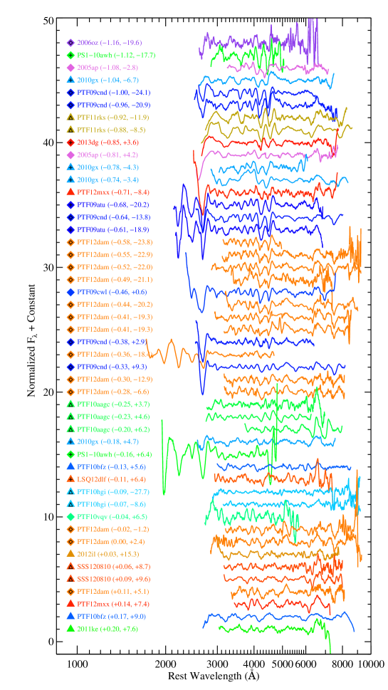
Figure 6: Spectroscopic sequence of SLSNe-I in spectral phase order from $\phi=-1.16$ to $+0.20$ (top to bottom). The spectra have been smoothed, continuum divided, and then scaled and shifted for clarity. The symbols next to the labels distinguish between events spectroscopically similar to PTF12dam (diamonds) and those more similar to SN 2011ke (triangles). We have added markers inside some of these symbols to help distinguish between symbols of similar color. The numbers in parentheses next to each object name are the spectroscopic phase and the light-curve phase in days, respectively.

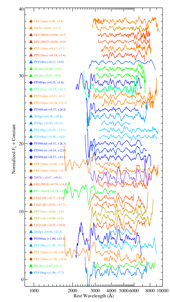
Figure 7: Similar to Figure 6 but for $\phi=0.00$ to $+1.09$.

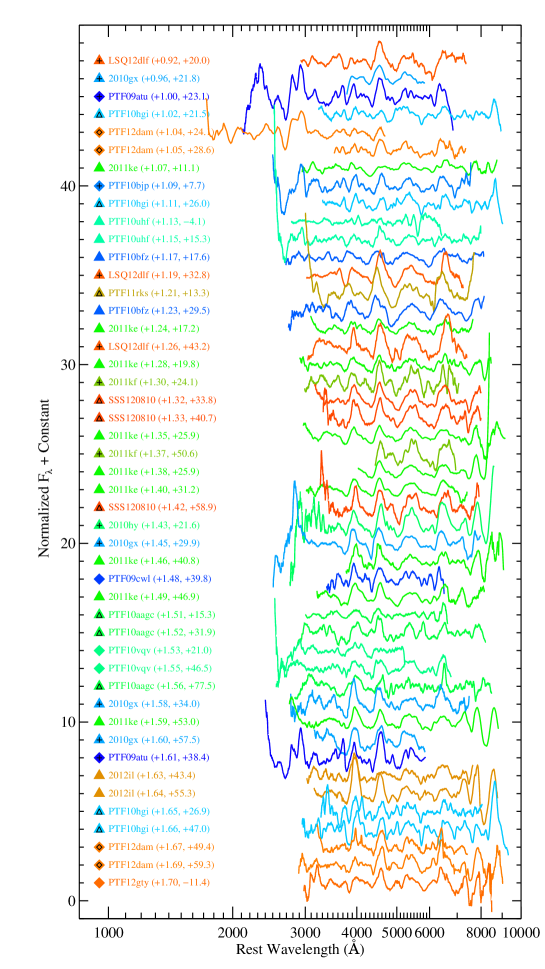
Figure 8: Similar to Figure 6 but for $\phi=+0.92$ to $+1.70$.

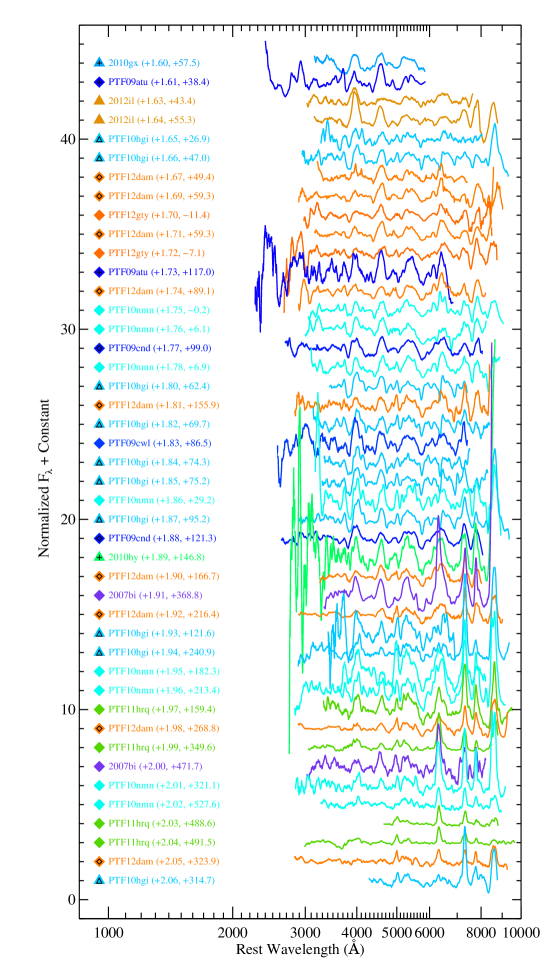
Figure 9: Similar to Figure 6 but for $\phi=+1.60$ to $+2.06$.

We arbitrarily assign a spectroscopic phase of $\phi=0$ to the $t=+2.4$ d spectrum of PTF12dam that was obtained around the time that the O II features had faded in strength, leaving a largely featureless spectrum. Next, we assign $\phi=1$ to the spectra of PTF09atu taken at a light-curve phase of $t=+23$ d. These data are found to be best matched by SN Ic templates, such as SN 1994I and SN 2004aw near photometric maximum. We assign $\phi=-1$ to the spectrum of PTF09cnd taken $\sim 24$ days before maximum light, which exhibits strong O II features. Last, we assign $\phi=2$ to the spectra of SN 2007bi from about 470 days after maximum light, in which nebular features are dominant. The spectra which fall within $-1<\phi<1$ are then assigned fractional phases such that the change, $\Delta\phi=\phi_{2}-\phi_{1}$, is roughly proportional to the difference in corresponding light-curve phases, $\Delta t=t_{2}-t_{1}$. SLSNe-I, like other SNe, tend to evolve more slowly as they age, and we choose to adopt a roughly logarithmic scaling, $\Delta\phi\propto\log\Delta t$, for $\phi>1$. In Table LABEL:table:speclog we give the fiducial spectral phases for the spectra composing the spectral sequence (Fig. 6-9).

Through template matching, we can now determine spectroscopic phases for any SLSN-I (or SN Ic) to the extent that these objects follow this single spectroscopic sequence. We cross-correlate each spectrum with all of the reference spectra to find the best matches and then calculate the spectroscopic phase from the average $\phi$ of the top 5 matches. The standard deviation of these values is used as an estimate of the uncertainty. For the cross-correlation, we focus on the 3200–7400 Å region, which is the best covered by our SLSN-I templates (Fig. 2). The calculated spectroscopic phase for each spectrum in the PTF SLSN-I sample is also given in Table LABEL:table:speclog.

4.1 SLSN-I Spectral Subgroups

During this template-matching procedure, we noticed that a number of objects were best fit by one list of comparison objects (including SN 2011ke, PTF10uhf, SSS120810), while a number of other objects were best fit by another set of comparison objects (including PTF12dam, PTF09cnd, PTF09atu). The set of objects that drew their best matches from both lists was surprisingly small. Motivated by this, we attempted to classify each SLSN-I as more similar to SN 2011ke or PTF12dam based on how frequently their spectra appeared together with SN 2011ke or PTF12dam in the top 5 matches. Table 5 shows the number of times that a given object was found in the top 5 matches with SN 2011ke and PTF12dam. To guard against spurious results we limited the search to the 152 spectra in our spectral sequence above. Objects that were not included in the spectral sequence, such as PTF09q, are listed in the table but were obviously never found in the top 5 due to this constraint. We find that there are 81 spectra that have a match to at least one PTF12dam spectrum in the top 5, and 56 spectra with at least one match in the top 5 to SN 2011ke, but there are only 10 spectra where both PTF12dam and SN 2011ke are found in the top 5 together.

We classify objects as spectroscopically more similar to SN 2011ke or PTF12dam based on how frequently a given object is in the top 5 matches of other objects with either SN 2011ke or PTF12dam (note that the arbitrary assignments of $\phi$ values above has no impact on the frequency of matches). To do this, we take the fraction of cases where the object is found in the top 5 with SN 2011ke or PTF12dam compared to the total number of spectra with these objects in the top 5. For example, PTF10aagc is in the top 5 with SN 2011ke for 4 out of 56 possible spectra ($\sim 7$% of the time), and it appears in the top 5 with PTF12dam 5 out of 81 possible spectra ($\sim 6$% of the time), so we tentatively place it in the SN 2011ke-like group. For objects that are not included in the spectroscopic sequence, we assign spectroscopic subgroups based on the frequency of matches to the other SN 2011ke-like and PTF12dam-like objects identified through the procedure above.

In Figures 6 to 9 we mark the SN 2011ke-like objects with triangles and the PTF12dam-like objects with diamonds. These figures show that the spectral sequence does not alternate randomly between SN 2011ke-like and PTF12dam-like spectra. Rather, there are continuous runs of one object type or the other. For example, the range $1.11<\phi<1.46$ consists of 21 SN 2011ke-like spectra and zero PTF12dam-like spectra. These spectral phases may thus be unique to the evolution of SN 2011ke-like objects. Another possibility is that PTF12dam was not well sampled over this range (our spectra contain a 3-week gap in coverage) and it is this lack of PTF12dam spectra over this $\phi$ range that drives the SN 2011ke-like versus PTF12dam-like division. We also note that 23 out of the 29 earliest phase spectra ($\phi<-0.28$) are PTF12dam-like events, but PTF12dam itself was well observed over this period and accounts for 10 of these spectra. Because of the lack of early-time SN 2011ke-like spectra and possible contamination from host light at late times, we have only considered spectra in the $-0.3<\phi<1.7$ range when assigning subgroups.

4.2 Spectral Evolution Rate of SLSN-I Subgroups

We next consider how the calculated spectral phases correlate with light-curve phase. For this comparison, we will use the standard definition of light-curve phase for hydrogen-poor SNe, which is the number of rest-frame days after optical maximum, often specifically referenced to the $B$ or $g$-band maximum. This is a convenient epoch to serve as a basis since it is quite often directly constrained by observations; however, it is not necessarily the most physically motivated choice. For comparison, hydrogen-rich SNe are typically indexed by days from explosion instead. In Figure 10 we show the dependence of spectral phase on light-curve phase for SLSNe-I and selected SNe Ib and SNe Ic (spectral phases for these normal-luminosity events are determined through cross-correlation to the SLSNe-I with assigned spectral phases as discussed above). We separate out the SLSN-I sample into PTF12dam-like, SN 2011ke-like, and objects that either have poorly constrained dates for maximum light or that were classified as possible SLSNe-I. The abscissa in Figure 10 is linear up to day 35 where it changes to a logarithmic scale.

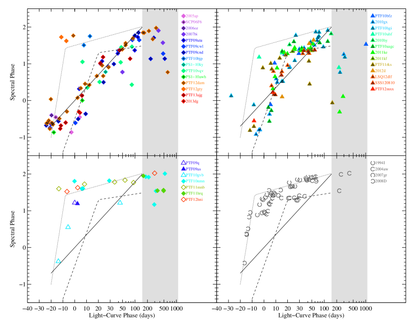
Figure 10: Spectral phase ($\phi$) versus light-curve phase ($t$) for the SN samples discussed in this paper. The gray shaded region marks phases where the spectral matching may fail owing to contamination from host-galaxy light. We show separately the PTF12dam-like sample (upper-left panel), the SN 2011ke-like sample (upper-right panel), the possible SLSNe-I and objects with poorly constrained light-curve phases (lower-left panel), and a few normal-luminosity SNe Ib and SNe Ic (lower-right panel). In each panel we plot possible trends for the PTF12dam-like sample (solid lines), the SN 2011ke-like sample (dashed lines), and the SN Ib/c sample (dotted lines) for reference. See text for further details.

Starting with the upper-left panel in Figure 10, we see that the PTF12dam-like events largely cluster along the diagonal in the figure. As discussed above, the numerical values for spectral phase are anchored to PTF09cnd, PTF12dam, PTF09atu, and SN 2007bi, which all belong to the PTF12dam-like group. It is perhaps then not a complete surprise to find this result, although this was by no means guaranteed. There is, however, a large amount of scatter in the relation. Part of this is caused by a high catastrophic failure rate in the simple cross-correlation method used to calculate spectral phases. For example, there are two observations of PTF12dam taken around maximum light. One of these is found through cross-correlation to have a spectral phase of $\phi=0.08\pm 0.34$, which agrees quite well with the definition of spectral phase above (PTF12dam should have $\phi\approx 0$ near maximum light). However, the second spectrum has a calculated value of $\phi=1.71\pm 0.27$, which is clearly discrepant. Examining the fitting results, it appears that a combination of factors including systematic error from the spectral extraction led to this discrepant value. Visual comparison confirms that this spectrum should have a spectral age of $\phi\approx 0$. Additionally, our cross-correlation technique does not account for host-galaxy contamination; thus, the calculated spectral phases can be bogus at late phases ($t>150$ d) when the SLSNe-I have faded to or below the background level. We retain the values of spectral phase determined automatically through the cross-correlation analysis described above and simply note that more advanced techniques are required to improve the robustness of spectral phase determination.

Despite the scatter, it is clear from the upper-right plot in Figure 10 that the SN 2011ke-like events chart a different course through the $t$ vs. $\phi$ plane than the PTF12dam-like events. These events navigate through the early spectral phases ($\phi<1$) more rapidly before they change tack and slowly approach the PTF12dam-like sequence at about $\phi=1.4$. We note that some of the PTF12dam-like objects may follow this trend at least at early times. SN 2005ap, for example, has just two spectra available, but these appear to follow the SN 2011ke-like trend better.

Moving to the lower-right plot in Figure 10, we see further distinction between normal-luminosity SNe Ib/c and SLSNe-I. The lower-luminosity events tend to have significantly larger spectral phases at earlier light-curve phases than do SLSNe-I. SN 2008D is the only object shown with spectral phases significantly less than $\phi=1$. It quickly moves through the spectral sequence, however, reaching $\phi\approx 1.5$ after its light curve’s maximum. SN 2004aw is also noteworthy for following a path that is not too dissimilar from that of SN 2011ke, especially 20–40 d after light-curve maximum. We note that PTF12gty is a considerable outlier from the PTF12dam objects in the $t$ vs. $\phi$ plane, and it may better fit with the normal-luminosity SNe Ib/c. This is especially interesting given the peak luminosity of PTF12gty, which is quite low compared to the other SLSNe-I but which would be rather high for a SN Ic. PTF10bjp also shows advanced spectral phases at relatively early light-curve phases, which may be more similar to the normal-luminosity SNe Ib/c shown.

Finally, the lower-left panel in Figure 10 shows objects from the possible SLSN-I sample and objects that have poorly constrained dates for photometric maximum. These all tend to favor larger spectral phases at younger light-curve phases than do most SLSNe-I in a manner similar to the SNe Ib/c shown. In the cases where the date of maximum light is poorly constrained, it could simply be the case that the true light-curve phase is significantly larger than shown; correcting these to the true values could then shift the observations to the PTF12dam or SN 2011ke-like tracks.

Table 5: SLSN-I Spectroscopic Groups

	In Top 5 With		Feature
Name	SN 2011ke	PTF12dam	Group
SN 2005ap	0	2	12dam-like
SCP06F6	0	0	12dam-likea
SN 2006oz	0	1	12dam-like
SN 2007bi	3	9	12dam-like
PTF09q	0	0	11ke-likea
PTF09as	0	0	11ke-likea
PTF09atu	11	26	12dam-like
PTF09cwl	8	20	12dam-like
PTF09cnd	8	34	12dam-like
PTF10bfz	10	3	11ke-like
PTF10bjp	3	7	12dam-like
SN 2010gx	16	14	11ke-like
PTF10hgi	5	3	11ke-like
PTF10gvb	0	0	11ke-likea
PTF10nmn	5	16	12dam-like
PS1-10ky	0	0	12dam-likea
PTF10uhf	6	4	11ke-like
PTF10vqv	1	4	12dam-like
SN 2010hy	8	8	11ke-like
PTF10aagc	4	5	11ke-like
PS1-10awh	0	0	12dam-likea
SN 2011ke	56	10	11ke-like
PTF11mnb	0	0	12dam-likea
PTF11hrq	3	9	12dam-like
SN 2011kf	4	0	11ke-like
PTF11rks	6	1	11ke-like
SN 2012il	7	4	11ke-like
PTF12dam	10	81	12dam-like
PTF12gty	1	14	12dam-like
LSQ12dlf	20	6	11ke-like
SSS120810	17	4	11ke-like
PTF12hni	0	0	12dam-likea
PTF12mxx	5	7	11ke-like
PTF13ajg	0	0	12dam-likea
SN 2013dg	0	2	12dam-like

^aTop spectral matches do not include PTF12dam or SN 2011ke, or the redshift is too high to match against these objects. In these cases the subgroup is assigned based on the subgroups of the best-matching templates.

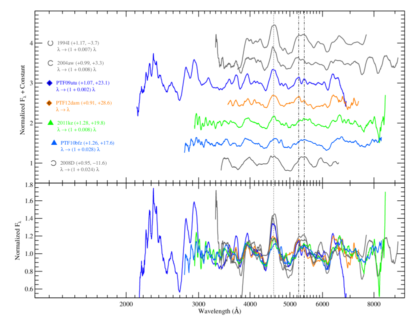
Figure 11: Spectra of SLSNe-I (colored lines) and SNe Ib/c (gray lines) at spectral phases close to $\phi=1$. Each spectrum has been shifted as indicated to best match the spectrum of PTF12dam in the 3500–5000 Å region (relative redshifts were determined through cross-correlation as described in the text). The vertical, dotted line marks a prominent peak near 4600 Å, and dash-dotted lines mark peaks seen near 5400 Å or redder in some cases.

5 Spectral Comparisons

We have shown that SLSNe-I can be spectroscopically distinguished from normal-luminosity SNe through template comparison and that SLSNe-I may further be divided into PTF12dam-like or SN 2011ke-like groups based on the relative frequency of good template matches to these objects. In this section we look for specific spectral features that may correlate with these divisions.

We begin by comparing in Figure 11 the near-maximum-light spectra of the normal-luminosity SNe Ic 1994I and 2004aw and the premaximum-light spectra of the normal-luminosity SN Ib 2008D with members of the SN 2011ke-like and PTF12dam-like SLSN-I groups, all at a similar spectral phase ($\phi\approx 1.0$). To align spectral features, we cross-correlate each spectrum in the 3500–5000 Å region to determine shifts, $\delta z$, relative to PTF12dam. In the figure, we plot wavelength on a logarithmic scale so shifting the spectral wavelengths by $\lambda\rightarrow(1+\delta z)\lambda$ is just a uniform displacement left or right as indicated by the locations of the plotted symbols.

The spectra displayed in Figure 11 show a number of similarities, but there are noticeable differences as well. For example, SN 2008D has a strong absorption feature at about 5700 Å, which is usually attributed to a blend of Na I and He I. This feature is more weakly present in SN 1994I but hardly noticeable in the other spectra. As is evident in the figure, stripped-envelope SNe comprise a heterogeneous class, and while it is possible to identify differences between specific events (e.g., one SN Ic versus another SN Ic or a SLSN-I), it is not clear from this comparison that there is a single defining feature that differentiates SNe Ic from SLSNe-I. Rather, the distinction discovered in §2 may be the result of a number of subtle features in combination, such as the relative weakness of line strengths in SLSNe-I compared to SNe Ic or small shifts of certain features with respect to others.

Figure 11 shows a possible distinction between SN 2011ke-like and PTF12dam-like events: when the spectral peaks at about 4600 Å are aligned, the broader peaks near 5400 Å extend further to the red in the SN 2011ke-like events shown in the figure. It also appears that the SN 2011ke-like events may have broader features. The limited wavelength ranges and small number of objects included in the comparison make it difficult to determine how significant this difference may be, however. In order to compare SN 2011ke-like and PTF12dam-like events, we therefore must look at the average spectral properties of each group over some range of spectral phases.

In Figure 12 we show the spectra of the SN 2011ke-like and PTF12dam-like subgroups at spectral phases near $\phi=-0.65$, 0.0, $+0.65$, and $+1.35$. The spectra are continuum divided and color coded by object. We also compute the average spectra for each group by using the modified Savitsky-Golay smoothing method discussed in Appendix A. To do this, we first compute the average for a given group of spectra and then determine the velocity shift for each component spectrum relative to this initial average. We then shift the individual spectra to align them before computing the final average spectrum.

As shown in the upper-left plot in Figure 12, the spectra of PTF12dam-like and SN 2011ke-like events at early spectral phases ($-1<\phi<-0.3$) are broadly similar, but there are some apparent differences. In the range 3000–5700 Å, the PTF12dam-like objects exhibit a number of features usually attributed to O II (see 6.1). In the average SN 2011ke-like spectrum, however, two of these features are missing and the absorption at 3600 Å appears broader. Looking back at Figure 6, we can see that the SN 2011ke-like event PTF11rks lacks the notches at about 3800 and 4000 Å, but these features are clearly detected in spectra of PTF09cnd and PTF09atu at similar spectral phases. The earliest spectrum of the SN 2011ke-like event SN 2010gx also lacks these notches, although they are present in the second spectral epoch. Additionally, these features are not clearly present in the PTF12dam-like event SN 2005ap. This raises the possibility that these notches may be transient features in both SN 2011ke-like and PTF12dam-like events, and perhaps they are not present at very early epochs. Another possibility is that SN 2005ap may be better associated with the SN 2011ke-like group (recall also that SN 2005ap may evolve more similarly to SN 2011ke-like objects through the $\phi$ vs. $t$ diagram in Figure 10).

There also appear to be strong differences in the average SN 2011ke-like and PTF12dam-like spectra at 7000–8000 Å over the $-1<\phi<-0.3$ range, although there is a paucity of SN 2011ke-like data available for the comparison. Nevertheless, the PTF12dam-like spectra show a broad absorption dip at $\sim 7500$ Å that is absent in the SN 2011ke-like sample, which in turn appears to show an absorption feature at 7800 Å that is missing in the PTF12dam-like sample. This difference is also seen in the $-0.3<\phi<0.3$ range shown in the upper right of Figure 12, although again there are few observations contributing to this comparison.

A second difference in the $-0.3<\phi<0.3$ range is that the SN 2011ke-like spectra are noticeably smoother than the PTF12dam-like spectra, on average. The spectra remain broadly consistent, so this difference may suggest that the SN 2011ke-like events have larger expansion velocities that wash out individual features more than PTF12dam-like events. This is suggested by the velocity shifts noted in Figure 11, although it is not clear how well the velocity widths of SLSN-I features correlate with expansion velocities (see §8).

In the spectral phase range $0.3<\phi<1.0$ (lower-left plot in Fig. 12), we again find a stronger 7500 Å feature in the PTF12dam-like sample. The emission feature at $\sim 6500$ Å may also be more pronounced in the PTF12dam-like sample. Echoing the result from Figure 11, we see that the emission peaks at 5200 Å align, but the P-Cygni profiles around 4400 Å are significantly offset from each other. This may suggest that the ratio of velocities between ions in PTF12dam-like and SN 2011ke-like ejecta might not be constant. This difference is not seen in the later-phase ($1.0<\phi<1.7$) spectra in the lower-right plot of Figure 12, except possibly in the 7500 Å feature, which is finally present in the SN 2011ke-like sample. However, there are limited PTF12dam-like observations covering this wavelength range and phase.

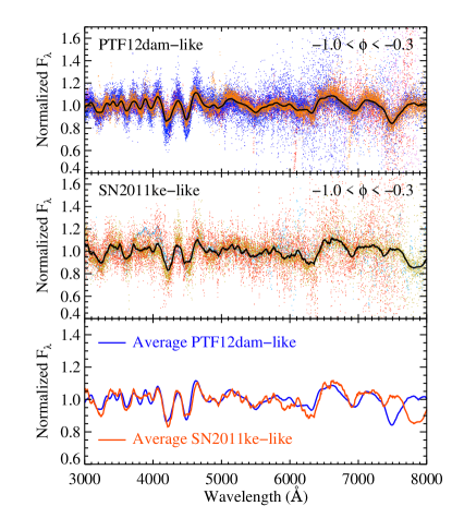
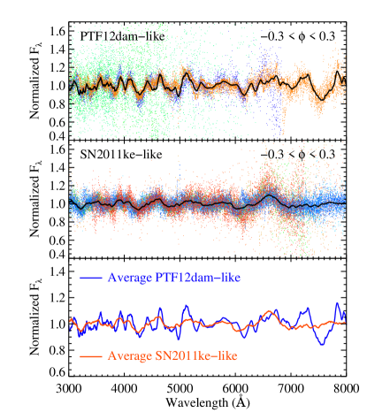
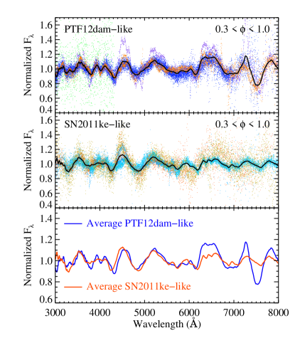
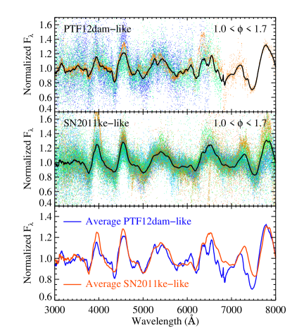
Figure 12: Average spectra of SLSNe-I with spectral phases in different ranges. Events deemed more spectroscopically similar to PTF12dam or SN 2011ke are shown in the top and middle panels of each plot, respectively. The spectra have been continuum divided. Dots show measurements from individual events (color coded as in Figs. 6–9), and the black lines indicate these combined data smoothed with a generalized Savitzky-Golay filter. The lower panel in each plot shows only these averaged spectra for comparison.

6 Spectral Line Identifications

In the above sections we discussed the spectral evolution of SLSNe-I in broad terms. In this section we attempt to identify the ions responsible for key features in the spectra. By associating specific features with specific ions, the composition and velocity structure of the atmosphere are revealed. Ideally, detailed radiative transfer calculations should be constructed and paired with a hydrodynamical code to self-consistently model spectral features as they evolve over time. However, such work is beyond the scope of this paper. We instead opt for a simplistic evaluation of line features, leveraging line identifications and numerical modeling in previous publications (Quimby et al., 2011; Dessart et al., 2012; Howell et al., 2013; Mazzali et al., 2016; Yan et al., 2017a). In some cases, we additionally use simple tools to test the validity of these features.

Two widely used tools for the identification of features in SN spectra are synow (Jeffery & Branch, 1990) and its more modern incarnation, syn++ (Thomas et al., 2011). These codes generate synthetic spectra for 1-D homologously expanding atmospheres with a distinct (or “sharp”) photosphere. A large number of parameters can be adjusted to create models of observational data. These parameters include photospheric velocity, ion species, ion temperature, and the relative contributions of different ions. However, the relative strengths of features arising from the same ion species are set by assuming local thermodynamic equilibrium (LTE). In this manner, potential line identifications can be tested by matching the model to a particular feature and then checking the agreement with any additional features predicted by the model.

One potential weakness of syn++ when dealing with multiple ion species is that in real SNe lines from different ions may form in different layers (and thus have different velocities). Although syn++ has the ability to “detach” ions from the photosphere, this adds further degrees of freedom to this already highly parametric modeling process. Also, the version of syn++ available can only model the ion distribution as an exponential function, and detached ions are thus computed for a physically unlikely structure (Gaussian distributions were not possible in the version available). Another weakness of syn++ is that it is not intended for use on spectra entering the nebular phase (where the assumption of a sharp photosphere breaks down), although it has been used to model relatively late-phase spectra (see Branch et al. 2008).

We have used syn++ to generate synthetic spectra similar to the average SLSN-I spectra at $\phi=-1$, $\phi=0$, and $\phi=+1$. These simple models are presented in Appendices F, G, and H, respectively. We find that the identities of some features suggested by previous works are problematic in that syn++ predicts additional features for these ions that conflict with the data. Below we reconsider the identifications of the principal SLSN-I spectral features in the photospheric phase. We defer study of the late-phase spectra to future work (see also Lunnan et al. 2016 and Jerkstrand et al. 2017).

6.1 Study of the O II Lines

The strongest features in the early-phase ($-1.0<\phi<-0.3$) spectra of SLSNe-I are two broad dips typically observed around 4200 and 4500 Å. These were first associated with blends of C III, N III, and O III (Quimby et al., 2007a), but these are now usually identified with a single ion, O II (Quimby et al., 2011). This latter identification was first made using synow, and it has gained wide acceptance owing to the fact that this single ion can account for both of the two major features as well as several weaker dips often observed from 3500 to 4000 Å. However, the simple models produced by synow with its default line lists also predict a relatively strong O II feature at $\sim 4000$ Å, which does not agree well with the data (observations do show a dip near 4000 Å, but it is typically weaker and shifted to the red of the predicted feature). Mazzali et al. (2016) have produced more advanced models that demonstrate O II can account for all of the major spectral features of early-phase SLSNe-I in the optical range, although a similar offset in the 4000 Å feature can be seen in their Figure 5.

The O II ion has not been detected in the spectra of any normal-luminosity SNe Ic. Aside from SLSNe-I, only the peculiar SN Ib SN 2008D (Soderberg et al., 2008; Mazzali et al., 2008; Modjaz et al., 2009) and the SN Ibn OGLE-2012-SN-006 (Pastorello et al., 2015) have shown spectroscopic evidence for this ion. For O II to be present, oxygen must be excited to a relatively high energy level (Mazzali et al., 2016). Thus, the lack of such observed features in normal-luminosity SNe Ic may simply be the product of rapid cooling through adiabatic expansion of initially compact progenitor systems, or due to a lack of nonthermal sources of excitation.

Figure 13 shows spectra of PTF09atu in the 3500–5000 Å range. Five features are labeled A–E (we assign the letter “A” to the reddest feature). To investigate which O II transitions contribute to each of the features, we downloaded all of the known O II lines from NIST. Expected relative intensities are calculated assuming the gas is in LTE at 15,000 K. We can then create a simple model spectrum where each of these lines is represented by Gaussian absorption functions with the same width. We can Doppler shift the lines by a uniform velocity and scale the line strengths by a uniform factor to match the observed spectra. Although this model does not properly account for the radiative transfer effects of an expanding atmosphere (e.g., we model lines as pure absorption features, whereas in reality each line should have a P-Cygni profile in accordance with the geometry of the system), the results provide a surprisingly good fit to the data (red dash-dotted line in Fig. 13). In fact, we recover a spectrum that is quite similar to syn++ models, including the offset of the O II “C” line at 4000 Å.

The failure of our simple absorption model to match the 4000 Å feature could mean that a second ion contributes to this part of the spectrum, or that the relative strengths of the individual lines in our model are inaccurate. To investigate this, we have identified in Figure 13 the transitions that contribute to each of the broad features in the spectrum. As can readily be seen, the O II features consist of a complex blend of many individual lines (see also Mazzali et al. 2016). In fact, most of the five major features are blends of two or more multiplets. For example, the “B” feature consists of transitions between the $3s\,^{4}P$ and $3p\,^{4}P^{0}$ levels and also transitions between the $3s\,^{2}P$ and $3p\,^{2}D^{0}$ levels. Looking at the “C” feature, we see that the absorption model predicts that the $3p\,^{4}D^{0}$ – $3d\,^{4}F$ transition should be dominant, but this disagrees with the data. If we artificially remove this transition, we find that the absorption model falls into excellent agreement with the data (blue dashed curve). We also note that the absorption model overpredicts the strength of the “A” feature. This is possibly connected to the failure of the “C” feature since they share a common energy level (the $3p\,^{4}D^{0}$ state). If we artificially weaken the contribution to the “A” feature by the same amount removed from the “C” feature, the overall model is in excellent agreement with the data. (In addition to the $3d\,^{4}F$ level, the $3p\,^{4}D^{0}$ level can also be populated from the $3d\,^{4}D$ level, which is involved in the transition for the C line, and the $3d\,^{2}P$ transition, which is responsible for the weak feature to the red of the A line.) It thus seems that the population of the $3p\,^{4}D^{0}$ state disagrees with the line intensities reported by NIST. In the original source it is noted that the $3p\,^{4}D$ transitions strengths were obtained through indirect means (Veres & Wiese, 1996). Thus, it is possible that these lines are weaker in nature than the published values suggest; given the importance of the O II, we suggest that a new laboratory investigation of its transitions is warranted.

Artificially removing/reducing the $3p\,^{4}D^{0}$ transitions as above, the effective wavelengths for the O II A–E blends are 4650.71 Å, 4357.97 Å, 4115.17 Å, 3959.83 Å, and 3737.59 Å, respectively, according to our simple absorption model assuming a temperature of 15,000 K.

In Figure 14 we show the O II features in the early-time spectra of several SLSNe-I. The figure includes three PTF12dam-like events (PTF09cnd, PTF09atu, and PTF12dam itself) and two other objects (SN 2010gx and PTF11rks) that we have tentatively grouped with SN 2011ke. For each of these spectra we fit our simple O II model with the $3p\,^{4}D^{0}$ transitions altered as described above to the B feature only and then show the predicted model spectrum at other wavelengths. We include an offset parameter in the model fits to account for possible errors in our determination of the continuum level.

We find that the fit to PTF12dam is excellent with the B feature actually resolved into its two multiplet components. Resolving this feature implies that the velocity distribution of O II is confined to a relatively narrow range. The best fit FWHM is $3800\pm 100$ km s^-1. The B feature is similarly resolved for PTF09cnd. For PTF09atu the formal fit favors a larger FWHM than we adopted in Figure 13; the best-fit continuum level for the model in this case is 20% higher than our data after dividing by the estimated continuum. If we assume our estimated continuum level is correct then the FWHM drops to 4200 km s^-1, but in this case the B feature should be resolved. The estimated and model continuum levels agree to $\sim 2$% for PTF12dam, and forcing the model to have a higher continuum level quickly washes out the two local minimum in the B feature, so the FWHM for this spectrum must be less than $\sim 4000$ km s^-1.

The FWHM of the O II features of the SN 2011ke-like objects in Figure 14 is similarly dependent on the true continuum level. Allowing the model continuum to rise $\sim 15$% above the estimated level, SN 2010gx and PTF11rks have FWHM of $11,500\pm 600$ km s^-1 and $9000\pm 2000$ km s^-1, respectively. However, if we fix the model continuum at the estimated level, the FWHM each drop to $\sim 4600$ km s^-1. Although the FWHM is strongly dependent on the estimated continuum level, the systematic velocities are not. These velocities typically agree to better than 500 km s^-1 as the continuum level is changed (this is also true for the PTF12dam-like objects in the figure).

The spectra of SN 2010gx and PTF11rks shown in Figure 14 are very similar despite a systematic velocity difference of 6000 km s^-1. The features are noticeably stronger in PTF11rks, but both objects have an O II E feature that is significantly broader than in the PTF12dam-like objects shown in the figure. Also, the C and D features in the model are not well matched to the SN 2011ke-like object spectra, but the two observed spectra are similar to each other over this wavelength range.

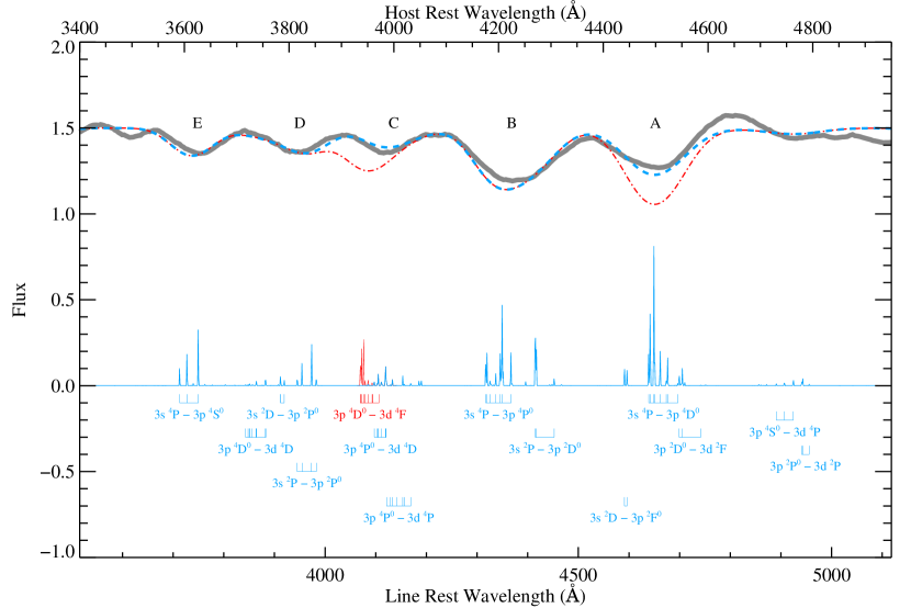
Figure 13: Transitions of the O II ion in the 3500–5000 Å range (thin blue lines) compared to continuum-divided spectra of PTF09atu (thick gray line). Relative strengths of each transition from NIST are shown assuming a 15,000 K plasma in LTE. Each multiplet is grouped and labeled. The lower abscissa indicates the laboratory wavelength for each transition while the upper abscissa shows wavelengths in the rest frame of PTF09atu’s host galaxy. The latter system is blueshifted with respect to the former by 10,000 km s^-1. The red, dot-dashed curve illustrates a synthetic spectrum created by Doppler broadening the multiplets (in absorption) by 7000 km s^-1 and scaling the result to match the observed PTF09atu spectrum. The blue dashed curve shows a similar synthetic spectrum but with the $3p\,^{4}D^{0}$ – $3d\,^{4}F$ multiplet (marked in red) removed and the $3s\,^{4}P$ – $3p\,^{4}P^{0}$ transition weakened as described in the text.

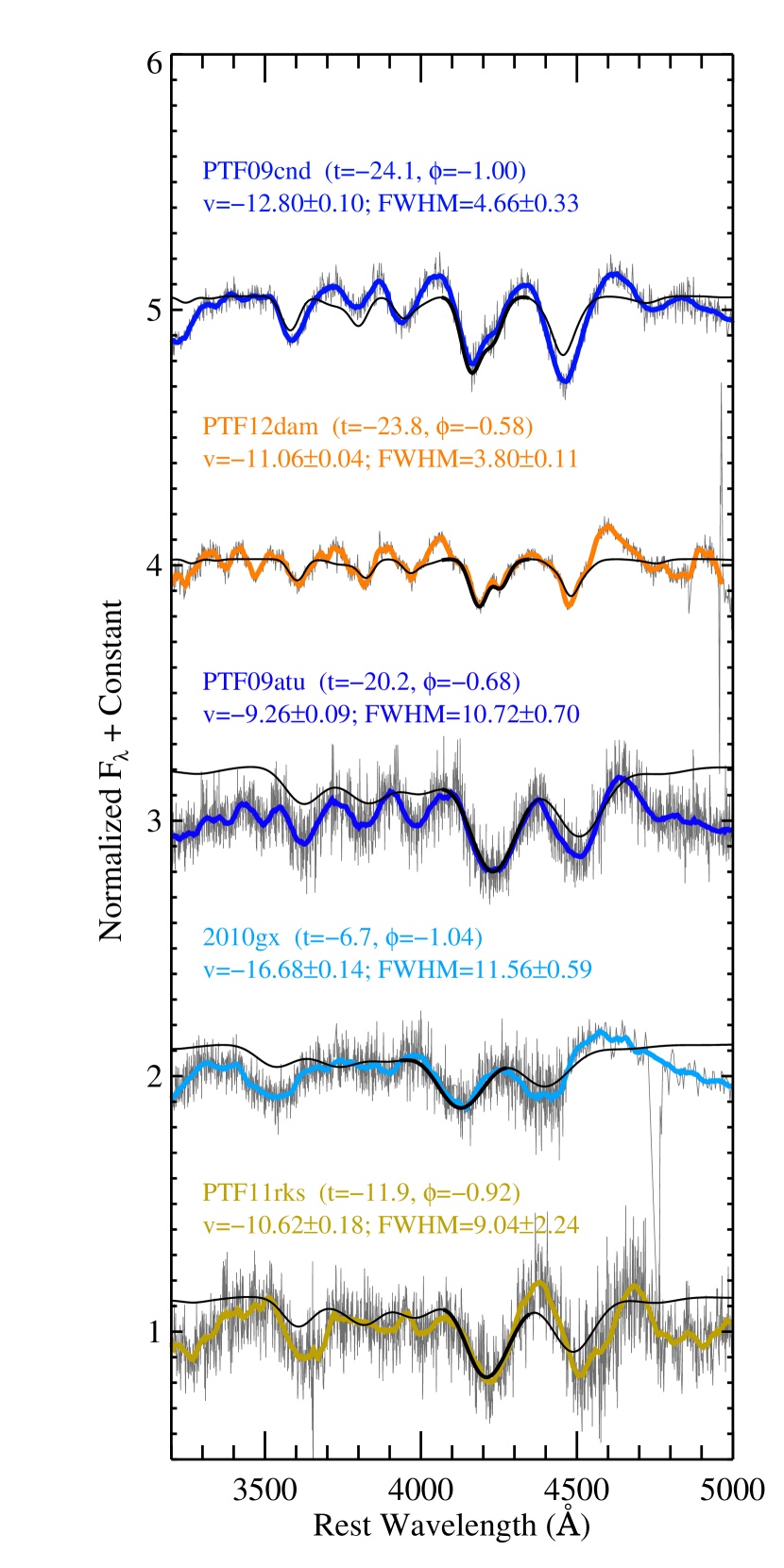
Figure 14: Early-phase spectra of several SLSNe-I highlighting the O II features. The spectra have been continuum divided and shifted for clarity. The smoothed data are shown with the thick colored lines. Best-fit velocities ($v$) and line widths of the multiplet components (FWHM) are given in 1000 km s^-1. The fit was limited to the “B” feature. We show the best-fit model with a thick black line and an extension of this fit to other wavelengths with a thin black line.

6.2 Spectral Features in the 5000–8000 Å Range

In Figure 15 we show spectra of PTF09cnd, PTF12dam, PTF10aagc, and PTF10bfz around maximum light in the 5000–8000 Å range. We have classified the first two of these objects as PTF12dam-like and the last two as SN 2011ke-like, although PTF10aagc is peculiar in that it exhibits hydrogen features (see §6.6). In the spectra of PTF09cnd we mark the expected locations of C II, Si II, and O I assuming a common velocity of 11,000 km s^-1. Each of these lines is well matched to clear local minima in the spectra, so we consider these identifications secure (see also Nicholl et al. 2016; Yan et al. 2017b).

The spectra of PTF12dam displayed in Figure 15 are very similar to the PTF09cnd spectrum, but the spectra of PTF10aagc and PTF10bfz lack clear evidence for the O I $\lambda 7774$ triplet. This was shown to be true for the average SN 2011ke-like spectrum presented in §5. The lack of O I $\lambda 7774$ around this phase could be a defining difference between PTF12dam-like and SN 2011ke-like objects, although we caution that there are relatively few spectra covering this wavelength range at the appropriate phases.

The absorption minimum near 5550 Å in the PTF09cnd spectrum plotted in Figure 15 could not be definitively identified. As we discuss in Appendix G, there are few ions that make strong features near this wavelength without producing stronger features that conflict with the observations. One possibility is C IV, but if this is indeed the case then the precise location of the minimum implies a velocity that is significantly ($\sim 3000$ km s^-1) faster than the other features noted in the figure.

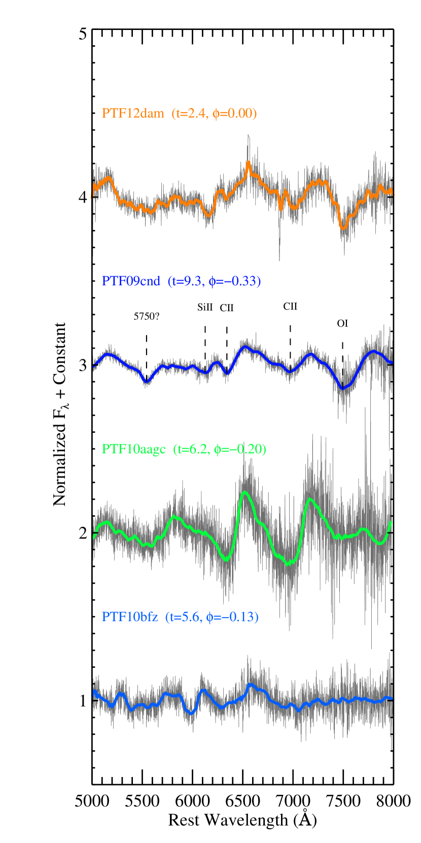
Figure 15: Spectra of four SLSNe-I around maximum light highlighting weak features in the 5000–10,000 Å range. Line identifications are given for PTF09cnd assuming a common blueshift of 11,000 km s^-1.

6.3 Spectral Features in the 1800–3500 Å Range

We now turn to the prominent spectral features in the near-UV band. Between 1800 Å and 2800 Å SLSNe-I typically exhibit four relatively strong dips at roughly 2650 Å, 2450 Å, 2200 Å, and 1950 Å. We will refer to these features as UV1, UV2, UV3, and UV4, respectively. Three of these lines were first identified through synapps fits as Mg II (UV1), Si III (UV2), and C II (UV3) by Quimby et al. (2011). Dessart et al. (2012) presented radiation-hydrodynamical calculations that produced these same identifications, but similar calculations by Howell et al. (2013) matched these features to blends of C II and Mg II (UV1); C II (UV2); C III and C II (UV3); and Fe III (UV4). They further find that the relative strengths of these features depend on luminosity. Mazzali et al. (2016) constructed synthetic spectral models for PTF13ajg and identify the four dips as C II and Mg II (UV1); Ti III, C II, and Si III (UV2); C III, C II, and Ti III (UV3); and Fe III and Co III (UV4). For another SLSN-I, SNLS-06D4eu, Mazzali et al. (2016) favor the identifications Mg II (UV1); Si III (UV2); C II (UV3); and Fe III (UV4). A consensus has yet to form on the ions responsible for these features or if the contributions change from one event to another, although most seem to agree that at least Mg II and C II are involved.

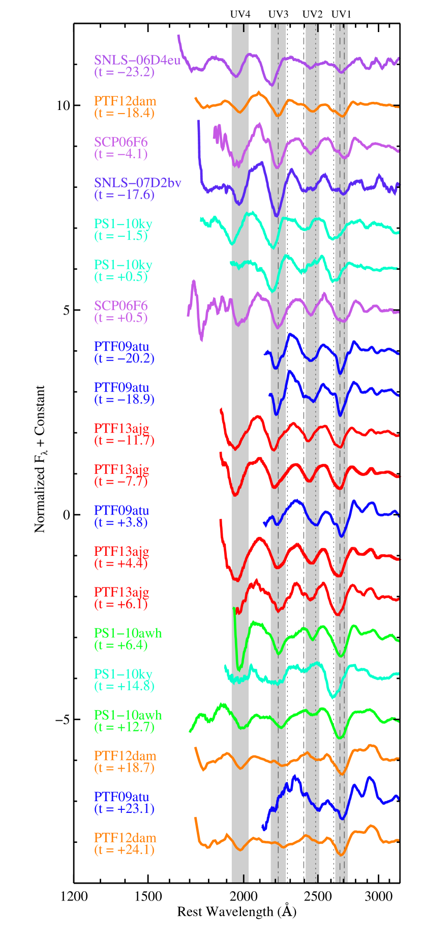
Figure 16: Smoothed and continuum-divided spectra of SLSNe-I in the near-UV range. SLSN-I spectra typically show four prominent features in this range, which are marked by the gray shaded vertical bands. The expected wavelengths of several strong lines (assuming a blueshift of 10,000 km s^-1, are marked by vertical lines: C II with dash-dotted lines, Mg II with dashes, and Fe II with dots. Phases given for the high-redshift, non-PTF targets are based on rest-frame UV photometry and may be biased with respect to the optically derived phases of the PTF targets.

These near-UV dips are not necessarily caused by the same ions at different phases or in different events. Some support for this is offered by Figure 16, which shows the near-UV spectra of several SLSNe-I at different phases. Inspection of this figure shows that while two different spectra may exhibit dips at similar wavelengths for one feature, other dips can be noticeably offset. For example, the spectra of SNLS-06D4eu and the earliest near-UV spectrum of PTF12dam both show an absorption dip near 2700 Å; however, the UV3 feature in PTF12dam is centered near 2220 Å while the closest corresponding feature in SNLS-06D4eu is centered closer to 2170 Å. This difference could mean that these UV3 features are the result of different ions or that the material responsible for this feature has a larger velocity in SNLS-06D4eu relative to other lines (assuming a rest wavelength near 2275 Å for each spectrum, the velocity difference would be $\sim 4000$ km s^-1). Interestingly, the later-time spectra of PTF12dam may reveal a weak dip at a wavelength similar to the UV3 absorption in SNLS-06D4eu. This may suggest that there are two (or more) ions contributing to the UV3 feature and that the relative strengths of these ions vary from event to event and with time. This especially may be the case for the UV2 feature, which shifts considerably more with time in the objects observed over sufficiently long temporal baselines (e.g., PTF09atu and PTF12dam).

To study possible line identifications for these UV features, we first consider the spectra of PTF09atu and PTF12dam — two SLSNe-I for which we have already identified spectral features in the optical. We can thus use the velocities found for the optical features to constrain the expected wavelengths of potential lines in the near-UV. As shown above, the optical lines of these SLSNe-I have low velocity dispersions, helping to resolve any blends into individual components. We present the evolution of the ion velocities in §7. One problem is that the velocities for ions in the optical are not measured at all phases (e.g., O II disappears around maximum light). Thus, we must sometimes extrapolate velocity measurements to earlier or later phases. We do this by fitting a simple linear model to the trusted measurements and evaluating this fit at the required epochs. This may underestimate velocities at early and late phases as the measured velocity of normal SNe are often observed to begin with relatively rapid declines before flattening out at later times.

Figure 17 shows the spectral evolution of PTF09atu in the near-UV. We first note that the UV1, UV2, and UV3 line profiles are complex; it is evident from the deeper, narrower UV1 absorption compared to the shallower, broader UV2 feature and the notches in the wings of these broad dips that these are the product of multiple, blended lines. In the top panel we have marked the expected positions of various line minima based on the optical O II velocities inferred from the cross-correlation method described in §7. The weak notches in the red side of the UV1 and UV3 features in the earliest spectra are well matched to the expected locations of C II $\lambda\lambda$2836, 2837 and $\lambda\lambda$2325, 2326, 2328 (respectively) at the same velocity as O II. Next we find that the location of the UV1 minimum is significantly to the blue of the expected Mg II minimum, assuming the same velocity as O II. There are two possible interpretations of this result: (1) the UV1 feature may not be dominated by Mg II, or (2) the Mg II line-forming region is at a systematically higher velocity than O II. In support of the first possibility, we note a slight inflection in the red wing of the UV1 feature precisely where we would expect to find Mg II if it had the same velocity distribution as O II. In support of the latter possibility, we cannot identify a better candidate to dominate the UV1 feature (see §6.4). Another notable feature in Figure 17 is the notch visible in all spectra on the blue wing of the UV1 feature. This notch shifts to the red over time, suggesting it is tracing the velocity distribution that evolves similar to O II, but with a rest wavelength near 2700 Å. As discussed below, we could not identify the ion(s) responsible for this feature. Finally, we note that similar to the ions proposed for the UV1 feature, the ions proposed for the UV3 feature are systematically offset to the red.

In the bottom panel of Figure 17 we plot the same spectra but consider a different velocity evolution — one following the optical Fe II lines — to predict where major features should land. In this case, the expected position of the Mg II doublet is better aligned with the minimum of the UV1 feature, although it is now offset somewhat in the other direction. That is, if this feature is dominated by Mg II, then it would seem that the velocity distribution of this ion is systematically shifted to lower velocities than Fe II, at least as inferred from the line minima. The weak inflection point observed around 2715 Å is now roughly matched by C II. The lines expected to contribute to the UV3 feature now agree more closely with the data; however, the various lines proposed for the UV2 feature are offset to the blue of the observed feature.

It seems likely from this one object that there are different velocity distributions for different ions, with O II and C II favoring lower velocities, and Fe II and Mg II favoring higher velocities. To see if this is unique to PTF09atu, we now consider the near-UV spectra of PTF12dam obtained with HST. Figure 18 shows these data; again, we mark line positions based on optical O II velocities in the top panel and optical Fe II velocities in the lower panel. The phases of observation are now different than for PTF09atu, but there are some similar results. The unknown notch on the blue edge of the UV1 feature is again present, although adopting the Fe II velocities, a slightly different rest wavelength is favored (2720 Å vs. 2740 Å for PTF09atu). The minimum of the UV1 feature is better tracked by Mg II using the Fe II velocities. In addition, the proposed lines for the UV2 feature tend to be systematically biased to the blue of the data. A key difference is that the UV2 feature in the earliest ($\phi=-0.36$) spectrum of PTF12dam is noticeably more narrow than the $\phi\approx-0.65$ spectra of PTF09atu. There is a clear notch in the first PTF12dam spectra to the blue of the UV2 feature around 2350 Å, which may be weakly present in the $\phi=-0.61$ spectra of PTF09atu.

We also show in Figure 18 the expected positions of strong Fe III features. According to NIST there are a number of Fe III lines around 2000 Å which should blend into two or three distinct features. However, the expected minima for these blends are poorly matched to the UV4 feature adopting either the O II or Fe II velocities. This result is in conflict with the synthetic syn++ spectra presented in the Appendix and with previous associations of this feature with Fe III (Howell et al., 2013; Mazzali et al., 2016).

Figure 17: Spectral evolution of PTF09atu in the near-UV region. The same three spectra are plotted in each panel, but the middle panel shows the data after division by the estimated continua. Vertical lines mark the expected positions of several lines based on the velocities derived from O II (top panel) and Fe II (bottom panel). The spectral phase ($\phi$), time since maximum light in days ($t$), and assumed line velocities in km  s^-1 are written to the right of the spectra.

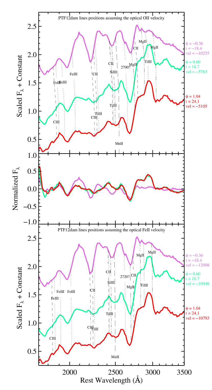
Figure 18: Similar to Figure 17 but for PTF12dam.

6.4 Possible Contributors to the UV Features

To consider possible line identifications for the notches observed around 2350 Å and 2600 Å, and to search for possibly different ions capable of contributing to the UV1, UV2, UV3, and UV4 features, we construct synthetic spectra using syn++. We compare these models to our HST UV grism spectra of PTF12dam to determine if a given species can produce lines at wavelengths appropriate to the data without generating strong features that are inconsistent with the data at other wavelengths. For our model spectra, we fix the photospheric velocity at 14,000 km s^-1 because this generates model O II spectra that are roughly consistent with the data (note that the positions of the line minima imply significantly lower velocities). We also fix the ion temperature at 10,000 K, but we also consider a set of synthetic spectra generated for 15,000 K ions as a check. The minimum and maximum velocities for each ion were set at 10,000 km s^-1 and 40,000 km s^-1, respectively, and the $e$-folding scale was set to 1.0. We then varied the reference line opacity to find the best match to the data.

After manually searching through all 83 ions in the syn++ library, we find the following possible contributors to the observed UV features: B IV, C II, O V, Mg I, Mg II, Al II*, Cr II*, Mn I, Fe II, and Fe IV* (UV1); B I, C I, C II, Mg I, Si III, P I, Ti III, V III*, Mn II, Fe I, Fe II, and Co II* (UV2); C II, C III, N IV, Co II*, Ni I, and Ba II (UV3); and B III, N II, Mg I, S II, Cr II*, Mn III*, Fe III (UV4). Asterisks mark cases where additional, strong features are predicted that at least partially disagree with the PTF12dam spectra. Detailed models are required to determine if any of these species are truly compatible with the observations. Many of these ions produce strong features at shorter wavelengths. Further observations constraining the far-UV spectra of SLSNe-I may prove useful in determining the true identifications of the near-UV spectral features (e.g., Yan et al. 2015).

6.5 Identification of Mn II

Again, the UV features are likely blends of multiple ions, and the relative strengths of these ions may ebb and flow as the spectra evolve. The most likely candidate for such a change in the dominant ion is the UV2 feature, which shifts significantly more to the red than do the other features. Most of the possible UV2 contributors listed above cannot explain the location of the UV2 minimum at later phases (e.g., the $\phi=0.60$ spectra of PTF12dam) without invoking impractically low velocities. We find that the best identification for the UV2 feature at these later phases is likely Mn II. This ion has a resonant transitions at 2576, 2593, and 2605 Å that agree well with the later-phase position of the UV2 line (assuming a velocity common to other lines; see Figures 17 and 18), and there are no stronger lines expected over the available data range. The spectra may also show Mn II $\lambda\lambda$2939, 2949 and a blend of Mn II $\lambda\lambda$3460, 3474, 3482, but these features are weaker and possibly blended with other ions. No strong lines are expected in the optical, but Mn II has possibly been detected in the near-infrared spectra of other SNe (e.g., Marion et al. 2009). The Mn may have been synthesized in the explosion or in the final burning stages of the progenitor star, or it may reflect the metallicity of the progenitor. This feature may thus yield constraints on the progenitor or burning during the explosion.

6.6 Evidence for Hydrogen and Helium

As previously noted, the spectra of SLSNe-I most closely resemble those of SNe Ic, which exhibit little to no hydrogen and helium in their spectra. We now examine our spectroscopic SLSN-I sample to search for any signs of these elements.

Previous works suggest possible links between SLSNe-I and hydrogen-rich or helium-rich events (Benetti et al. 2014; Inserra et al. 2016b; see, however, possible host differences noted by Leloudas et al. 2015b and Perley et al. 2016). These include the high-luminosity SN 2008es, which exhibited broad hydrogen features in its spectra but without the narrow emission lines characteristic of SNe IIn and other SLSNe-II (Miller et al., 2009; Gezari et al., 2009). It has been suggested that SN 2008es may actually be a relative of SLSNe-I that retained some of its hydrogen envelope at the time of its explosion. There have also been SLSNe-I reported that appeared hydrogen poor at maximum light but which developed hydrogen emission lines in their late-phase spectra (Yan et al., 2015, 2017b). For these objects, it is possible that the hydrogen detached from the progenitor just prior to the SN explosion. In this scenario helium should also be expected to be present, and it is perhaps present in other SLSN-I atmospheres as well. There have been reports of helium in the spectra of the SLSN-I SN 2012il (Inserra et al., 2013), but analysis of the spectra shows that the feature proposed to be He I $\lambda 10830$ is actually significantly offset to the red (see Appendix D); thus, this feature is unlikely to be He I.

We visually inspected the spectral time series for each of our SLSNe-I to look for signs of hydrogen. This is complicated by the potential presence of other ions that may produce features at similar wavelengths. In particular, C II $\lambda\lambda$6578.05, 6582.88 and $\lambda\lambda$7231.33, 7236.42 bracket the expected location of H$\alpha$ emission. Together, the P-Cygni profiles from these lines can potentially mimic the presence of H$\alpha$ (the 6578–82 doublet in particular could form a P-Cygni feature very close to what might be expected for H$\alpha$). In Figure 19 we show the spectra of PTF12dam at $t=-22$ d ($\phi=-0.52$) with the possible locations of these C II features marked assuming a blueshift of 12,000 km s^-1 (see also Fig. 15). Vertical dashed lines mark the rest wavelengths of H$\alpha$ and H$\beta$. While there is a possible broad emission feature roughly centered where H$\alpha$ would be, the absorption dips to either side of this are well matched by C II at a velocity similar to the O II lines discussed in §6.1 and the C II features discussed in §6.3. Thus, it is not clear if hydrogen is required to explain the spectra of PTF12dam.

Figure 19 also shows spectra of PTF10aagc at an early ($\phi=-0.20$) and later ($\phi=+1.56$) phase. In this case the emission peak near H$\alpha$ is much stronger in the early-phase data. In the later-phase spectrum, there is an emission feature slightly blueshifted from rest H$\alpha$ similar to what has been observed for other SLSNe-I with late-time hydrogen emission (Yan et al., 2015, 2017b). This offset is seen for both H$\alpha$ and the weaker H$\beta$ line, which is apparent in the smoothed data as well. We thus conclude that at least some hydrogen is present in the envelope of PTF10aagc at the time of explosion. The later-phase spectra of PTF12dam do show broad emission to the blue of rest H$\alpha$; however, the line center implies a blueshift of 6000 km s^-1, which tends to exclude this possibility. An alternative identification is [O I] $\lambda\lambda$6300, 6364, although the observed feature is shifted to the red of this. We also note that the later spectra of PTF12dam show a broad absorption minimum near 7550 Å, which we identified as the O I $\lambda$7774 triplet. This feature appears to be absent in the PTF10aagc spectra, perhaps consistent with more envelope stripping in the case of PTF12dam (see Sun & Gal-Yam 2017 and references therein). Spectra of other SLSNe-I do not provide clear evidence for hydrogen. The late-phase spectra of SN 2011ke do appear to show a broad feature centered at the wavelength of H$\alpha$ (see Fig. 34 in Appendix E), but these spectra are dominated by host-galaxy light and it is possible that this feature is simply made from the wings of the H$\alpha$ profile from the host.

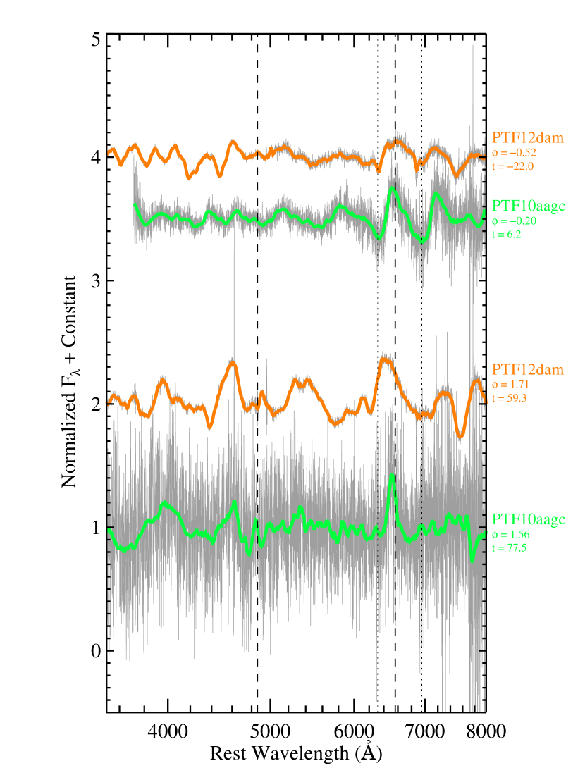
Figure 19: Continuum-divided spectra of PTF12dam and PTF10aagc with the rest wavelengths of H$\alpha$ and H$\beta$ marked with vertical dashed lines and the expected positions of 12,000 km s^-1 blueshifted C II lines marked with vertical dotted lines. Smoothed versions of the spectra are plotted with the thick colored lines.

We examined the temporal series of spectra of our SLSN-I sample and find one case where helium is clearly detected. PTF10hgi not only shows a much stronger absorption feature near 5750 Å (which is sometimes identified as blueshifted He I $\lambda 5875$ but can be blended or dominated by Na I D) compared to other SLSNe-I, but it also exhibits absorption dips at a consistent velocity for the 6678, 7065, and 7281 Å lines of He I. In Figure 20 we compare the spectra of PTF10hgi to the peculiar SN Ib 2005bf (e.g., Folatelli et al. 2006). He I lines show up clearly in the spectra of PTF10hgi by $t=+15$ d ($\phi=0.45$) and they persist until at least $t=+95$ d ($\phi=1.87$). Some other SLSNe-I may show weak evidence for one or two of these lines, but the presence of helium in these other cases is far less definitive. For example, the spectra of SSS120810 show possible He I $\lambda$7065 and He I $\lambda$7281 lines blueshifted by about 12,000 km s^-1, but if the 5875 Å feature is present it is rather weak. PTF10aagc also shows a relatively strong feature around 5550 Å in its $\phi=-0.20$ spectrum that could be He I $\lambda$5875 blueshifted by about 15,000 km s^-1. However, this feature could be from another line (e.g., Na I D), and it is unclear if the other He I lines are detected or if the features at roughly the appropriate wavelengths are the result of other ions such as C II (see also Yan et al. 2017b).

Strong helium lines appear to be a unique feature of PTF10hgi. For comparison, we show spectra of PTF12dam in Figure 20 at similar phases to the PTF10hgi spectra. Similar to SSS120810, in the $t=+57.8$ d ($\phi=1.71$) spectrum of PTF12dam there are dips around 6900 and 7100 Å that might suggest the presence of helium, but the expected He I $\lambda 5875$ feature is weak or absent. There are also other possibilities for the potential He I features including contributions from C II, O I, or a false absorption feature created by the emerging nebular lines of O I and Ca II.

Folatelli et al. (2006) have argued that the 6260 Å dip in the spectra of SN 2005bf shown in Figure 20 is high-velocity H$\alpha$. Spectra of PTF10hgi contain a similar feature that strengthens up to the $t=+95$ d spectrum before subsiding. However, for PTF10hgi the minimum of the dip is closer to 6350 Å. It is possible that this, too, is H$\alpha$ with an absorption minimum velocity merely 3000 km s^-1 faster than the He I lines (instead of $\sim 7000$ km s^-1 faster for SN 2005bf). This identification is supported by the detection of possible H$\beta$, H$\gamma$, and H$\delta$ lines at a similar velocity. The spectra of PTF10hgi bear a striking resemblance to those of the Type IIb SN 1993J, which also shows hydrogen lines offset to higher velocities than its helium lines (Barbon et al., 1995). We consider the identification of hydrogen and helium in the spectra of PTF10hgi secure, and these features remain clearly visible in the spectra for months. Thus, PTF10hgi may be the first example of a SLSN-IIb.

Our automated classification system may merely have flagged PTF10hgi as a SLSN-I owing to a lack of SN IIb comparison templates. But the PTF10hgi spectra do show some resemblance to those of SLSNe-I and SNe Ic. Nine of the eleven PTF10hgi spectra have $\Delta I_{\rm Ic-Ib}$ scores that favor classification as a SN Ic over a SN Ib. But again, based on the traditional classification scheme, the clear presence of hydrogen and He I lines should result in a SN IIb classification.

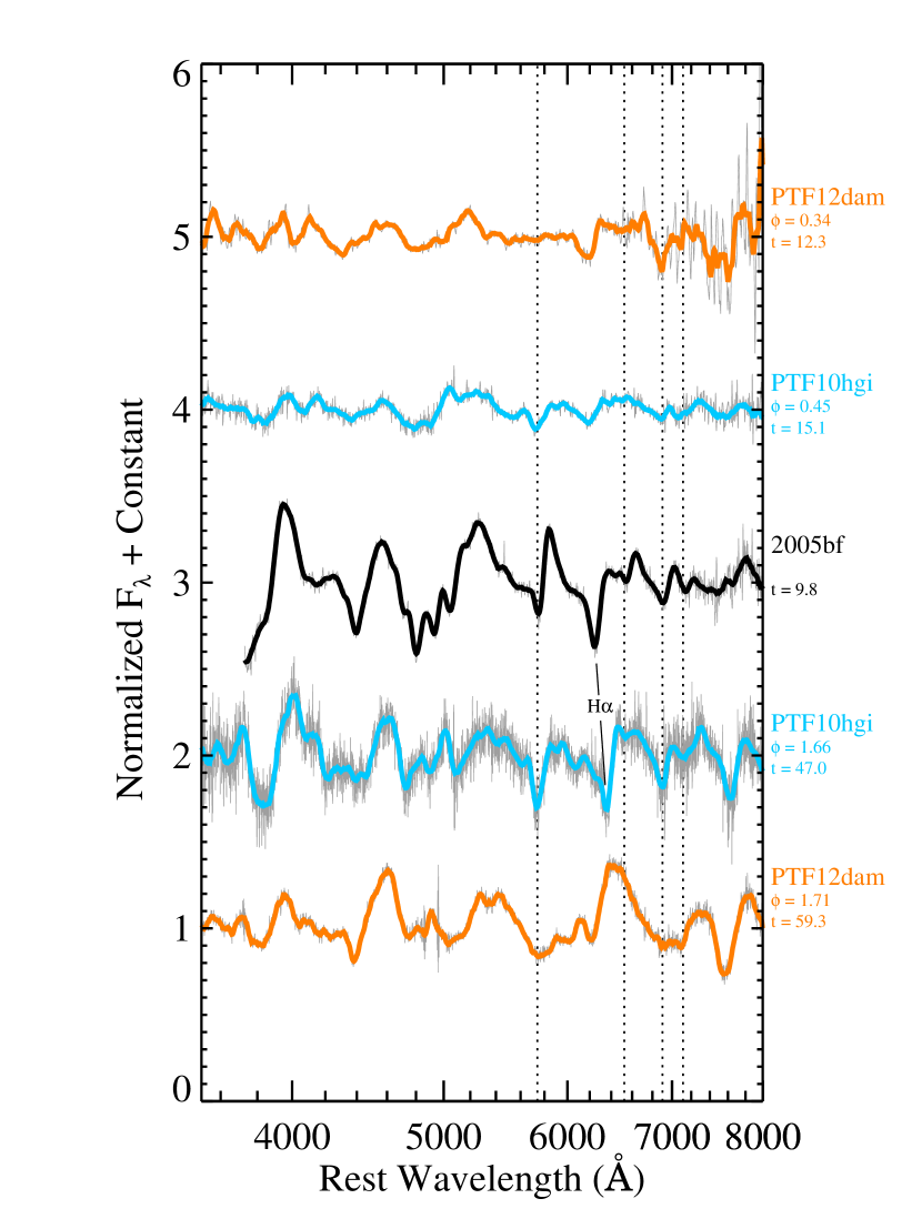
Figure 20: Spectra of the SN Ib 2005bf compared to the SLSNe-I PTF10hgi and PTF12dam. The spectra have been continuum divided, and the thick lines plot smooth versions of the data. The vertical dotted lines mark the expected position of prominent He I lines assuming a blueshift of 7000 km s^-1. All four of these lines are clearly detected in the SN 2005bf spectra and they can also be seen in PTF10hgi. However, the presence of He I lines in the PTF12dam spectra is less obvious.

7 Velocity Measures

In principle, the velocity structure of the ejecta can be determined through multi-epoch spectroscopic measurements. Since SNe produce broad P-Cygni profiles, it is common to measure the wavelength of the absorption trough (the minimum of the line profile) and to quote an ion’s absorption velocity using the known rest wavelength of the line and the (relativistic) Doppler formula. For SLSNe-I this procedure is complicated by two facts. First, the line features are very weak in comparison to those of normal-luminosity SNe. Second, there are multiple, blended lines present and unknown velocities that make association of a rest wavelength with any particular feature troublesome. Thus, in practice it is more difficult to assign velocities to particular ions from the spectra of SLSNe-I than for SNe Ic (see for example Liu et al. 2016).

For normal-luminosity SNe it is common to quote Fe II velocities based on the absorption minimum of the 5169 Å feature. This line is clearly detected in normal SN spectra and can be readily identified by the presence of two other Fe II lines at 4923 Å and 5018 Å. Usually the 5169 Å line is the strongest of these three, and it has been determined to be a good tracer of the photospheric velocity (Dessart & Hillier, 2005). However, this is not always the case. In SNe Ic the 5169 Å line is sometimes weaker than the two bluer lines, or the three may be blended together into a single, broad dip (Modjaz et al., 2014). It is possible for these lines to form above the photosphere and thus give a biased measure of the true photospheric velocity.

We have attempted to measure Fe II absorption velocities from the spectra in our sample, but clear measurements are not always possible given the difficulties mentioned above. We therefore attempt to measure velocities using several techniques and present the values obtained from each of these to give a sense of the systematic errors in these measurements.

We focus our discussion of velocity measurements on PTF12dam, which has excellent spectral coverage. The first technique we attempt is to identify the Fe II $\lambda\lambda$4923, 5018, and 5169 triplet by eye and then fit second-order polynomials to the data near each minimum. In the spectra taken near maximum light (spectroscopic phases $-0.3<\phi<+0.11$), all three of these lines can be clearly resolved. The formal fits result in relative velocity offsets of $\sim 500$ km s^-1. This is consistent enough that we feel confident identifying these features as the Fe II triplet. Some of the earlier-phase data also show one or two absorption features that appear to correspond to Fe II triplet components, but we note that the data are possibly contaminated by other features. At later phases the lines blend together. This may indicate an increase in the velocity width of the features. Also, the 5169 Å line appears to weaken relative to the two bluer components. In general, the 5169 Å feature does not appear to dominate this region of the spectra, implying that previous measurements that assumed the minimum of the broad feature corresponds to the 5169 Å line may be systematically in error (Modjaz et al., 2014). The 5018 Å feature may be the best tracer of the Fe II ion velocity in this case.

In Table 6 we present the velocities for PTF12dam as measured individually from each of the Fe II triplet components. There is considerable scatter for individual lines (around 500 km s^-1), but the data favor Fe II velocities of about $-11,500$ km s^-1 at the earliest epochs and a possible decline to lower blueshifts over time. The last epoch for which we find a reasonably well-resolved Fe II line minimum ($t\approx+59$ days) suggests a sudden drop in Fe II ion velocity to about $-10,500$ km s^-1.

Table 6: PTF12dam Fe II Absorption Minimum Velocities

LC Phase (d)	Fe II $\lambda$4923	Fe II $\lambda$5018	Fe II $\lambda$5169	Model	Cross-Correlation
$-23.8$	$-11.16$	$-11.64$	$-11.25$	$\cdots$	$-12.15$ $\pm 0.04$
$-22.9$	$\cdots$	$\cdots$	$\cdots$	$-13.10$	$-12.15$ $\pm 0.43$
$-22.0$	$-11.05$	$\cdots$	$\cdots$	$-12.54$	$-12.78$ $\pm 0.10$
$-21.1$	$-11.80$	$-12.16$	$\cdots$	$-11.91$	$-11.85$ $\pm 0.65$
$-20.2$	$\cdots$	$\cdots$	$\cdots$	$-11.69$	$-11.88$ $\pm 0.70$
$-19.3$	$\cdots$	$\cdots$	$\cdots$	$\cdots$	$-11.14$ $\pm 0.26$
$-19.3$	$\cdots$	$\cdots$	$\cdots$	$-11.49$	$-12.03$ $\pm 0.07$
$-18.4$	$\cdots$	$\cdots$	$\cdots$	$\cdots$	$-12.93$ $\pm 0.40$
$-12.9$	$\cdots$	$-12.28$	$-11.83$	$-12.10$	$-11.55$ $\pm 0.18$
$-6.6$	$-11.06$	$-11.37$	$-10.48$	$-11.27$	$-11.02$ $\pm 0.19$
$-1.2$	$\cdots$	$\cdots$	$\cdots$	$-12.03$	$-12.63$ $\pm 0.22$
$+2.4$	$\cdots$	$-11.67$	$-11.76$	$-11.76$	$-11.76$ $\pm 0.11$
$+5.1$	$-11.04$	$-11.34$	$\cdots$	$-10.79$	$-11.05$ $\pm 0.31$
$+8.7$	$\cdots$	$\cdots$	$\cdots$	$\cdots$	$-11.11$ $\pm 0.13$
$+12.3$	$\cdots$	$\cdots$	$\cdots$	$-9.96$	$-10.57$ $\pm 0.38$
$+18.7$	$\cdots$	$\cdots$	$\cdots$	$\cdots$	$\cdots$
$+23.2$	$\cdots$	$\cdots$	$\cdots$	$\cdots$	$-11.55$ $\pm 0.31$
$+24.1$	$\cdots$	$\cdots$	$\cdots$	$\cdots$	$\cdots$
$+28.6$	$\cdots$	$-11.34$	$\cdots$	$-10.88$	$-9.94$ $\pm 0.28$
$+49.4$	$\cdots$	$-11.29$	$\cdots$	$-10.02$	$\cdots$
$+59.3$	$\cdots$	$\cdots$	$\cdots$	$\cdots$	$\cdots$
$+59.3$	$-10.70$	$-10.21$	$\cdots$	$\cdots$	$\cdots$

All velocities are in units of $10^{3}$ km s^-1. Fe II $\lambda\lambda$4923, 5018, 5169 velocities are measured from second-order polynomial fits to the local absorption minimum. Model velocities are from a simultaneous fit to a simple Fe II absorption model (see text for details). Cross-correlation velocities are relative to the $+2.4$ d spectrum, which is assumed to have a blueshift of 11,760 km s^-1 based on the model fit. Uncertainties in the cross-correlation velocities are from Monte-Carlo tests and represent statistical uncertainties only.

We next attempt to measure Fe II ion velocities from the PTF12dam spectra by fitting a simple model to the spectra. The model is created using the wavelengths and relative intensities of Fe II lines from NIST assuming a 10,000 K plasma in LTE. Each line is represented by a Gaussian. Similar to the analysis in §6.1, the wavelengths of the lines are shifted using the relativistic Doppler formula, and the line widths and absolute intensities are fitted parameters (applied equally to all lines). The models are fit to the flattened spectra in the 4600–5200 Å range. Visual inspection suggests that the near-maximum-light ($t=+2.4$ day; spectroscopic phase $\phi=0$) spectra show three features with minimum reasonably matched to our simple model with a blueshift of 11,760 km s^-1. Although the overall fit is imperfect, the location of the minimum is relatively robust. We can compare this blueshift to the velocities found by fitting the 5018 and 5196 Å lines individually, which are 11,640 and 11,780 km s^-1, respectively. This supports an Fe II absorption velocity of about 11,700 km s^-1 at maximum light for PTF12dam. The FWHM of the fit is dependent on the local continuum (see §6.1) and the 5018, and 5169 Å lines appear to be blended with other features, but the 4923 Å line suggests a FWHM of less than 5000 km s^-1. Some of the additional PTF12dam spectra can be adequately fit using this simple model, but the model fitting breaks down when the three primary features are not all clearly detected. The best-fit values are presented in Table 6.

An alternative technique is to measure the velocity difference between two spectra directly using cross-correlation (e.g., Modjaz et al. 2014). This gives the relative velocity shift between the spectra, but if one of the input spectra has a known velocity measured from the techniques above, this can be added to the relative shift to determine the absolute velocity. In Figure 21 we show spectra of PTF12dam in the 4500–5300 Å range to highlight the Fe II features. We select the spectrum taken near maximum light and cross-correlate this against the other spectra shown in the figure to determine the relative velocity shifts. The dashed-dotted lines show the maximum-light spectrum shifted according to the cross-correlation results for comparison. There is clear evolution in the line features over the time interval considered. At early times the emission peak from the O II P-Cygni profiles likely affects features at shorter wavelengths, and at later times the emerging Mg II emission likely overwhelms the Fe II 5169 Å absorption. Nonetheless, the cross-correlation appears satisfactory until $t=+29$ days. Assuming the reference spectrum has a velocity of 11,760 km s^-1, we give the cross-correlation velocity evolution in Table 6.

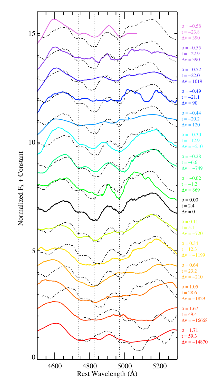
Figure 21: Spectra of PTF12dam highlighting the region of Fe II $\lambda\lambda$4923, 5018, 5196. Thick curves are the smoothed and flattened data. The right margin shows the spectroscopic phase ($\phi$), light-curve phase ($t$), and velocity shift ($\Delta v$) in km s^-1 relative to the maximum-light spectrum in black (positive values mean greater blueshifts). The dash-dotted lines show the maximum-light spectra shifted by the relative velocity found through cross-correlation. The vertical dotted lines mark the positions of the Fe II lines in the maximum-light spectrum for reference ($v_{\rm abs}=11,760$ km s^-1).

We can use the same techniques to measure the velocity evolution of O II. The measurements for PTF12dam are given in Table 7 and the cross-correlated spectra are shown in Figure 22.

Table 7: PTF12dam O II Absorption Minimum Velocities

LC Phase (d)	O II E	O II D	O II C	O II B	O II A	Model	Cross-Correlation
$-23.8$	$-10.72$	$-11.01$	$-10.76$	$-11.97$	$-11.37$	$-11.10$	$-11.10$ $\pm 0.02$
$-22.9$	$-10.11$	$-10.41$	$-10.77$	$-11.91$	$-11.53$	$-10.96$	$-10.89$ $\pm 0.22$
$-22.0$	$-10.39$	$-10.93$	$-10.36$	$-11.66$	$-11.38$	$-10.83$	$-10.86$ $\pm 0.03$
$-21.1$	$-10.49$	$\cdots$	$-9.96$	$-11.68$	$-11.30$	$-10.37$	$-10.83$ $\pm 0.28$
$-20.2$	$-9.73$	$-10.40$	$\cdots$	$-11.42$	$-11.08$	$-10.31$	$-10.68$ $\pm 0.31$
$-19.3$	$-9.69$	$-11.21$	$-10.14$	$-11.49$	$-11.17$	$-10.76$	$-10.62$ $\pm 0.04$
$-19.3$	$-11.07$	$-10.85$	$\cdots$	$-11.72$	$-11.33$	$-10.50$	$-10.35$ $\pm 0.09$
$-18.4$	$-12.20$	$-10.45$	$-9.88$	$-9.71$	$-9.10$	$-10.04$	$-10.20$ $\pm 0.20$
$-12.9$	$-9.54$	$-10.49$	$-8.53$	$-10.87$	$-10.92$	$-10.21$	$-10.08$ $\pm 0.14$
$-6.6$	$-8.30$	$-10.41$	$-8.00$	$-7.73$	$\cdots$	$-8.04$	$-8.68$ $\pm 0.21$
$-1.2$	$-7.07$	$-10.29$	$-8.38$	$-7.52$	$-7.34$	$-6.98$	$-8.27$ $\pm 0.29$
$+2.4$	$\cdots$	$-7.97$	$-7.60$	$-7.48$	$-6.88$	$-6.84$	$-7.76$ $\pm 0.17$
$+5.1$	$-8.59$	$\cdots$	$-7.52$	$\cdots$	$\cdots$	$-5.88$	$-8.59$ $\pm 0.41$
$+8.7$	$-6.44$	$\cdots$	$-7.45$	$\cdots$	$-6.77$	$\cdots$	$-7.17$ $\pm 0.10$
$+12.3$	$-8.62$	$\cdots$	$-7.49$	$\cdots$	$-6.11$	$\cdots$	$-8.74$ $\pm 1.26$

All velocities are in units of $10^{3}$ km s^-1. Velocities for O II E, D, C, B, and A are measured from second-order polynomial fits to the local absorption minimum assuming rest wavelengths of 3737.59 Å, 3959.83 Å, 4115.17 Å, 4357.97 Å, and 4650.71 Å, respectively. Model velocities are from a simple absorption model to the O II B feature (see text for details). Cross-correlation velocities are relative to the $-23.8$ d spectrum, which is assumed to have a blueshift of 11,060 km s^-1 based on the model fit. Uncertainties in the cross-correlation velocities are from Monte-Carlo tests and represent statistical uncertainties only.

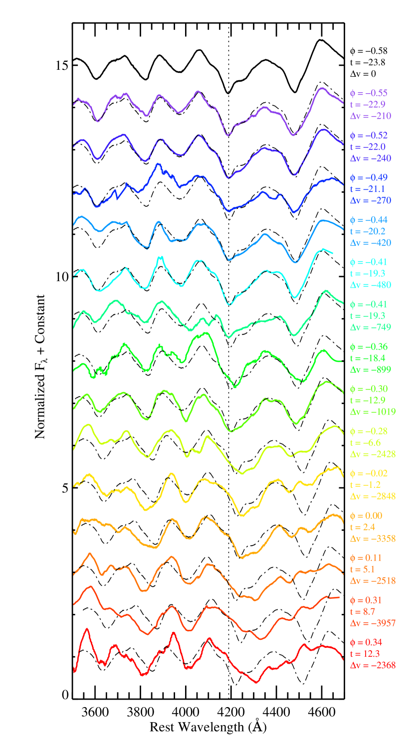
Figure 22: Similar to Figure 21 but highlighting the O II multiplets in the time-series spectra of PTF12dam. The vertical dotted line marks the position of the O II “B” line in the first spectrum for reference ($v_{\rm abs}=11,100$ km s^-1).

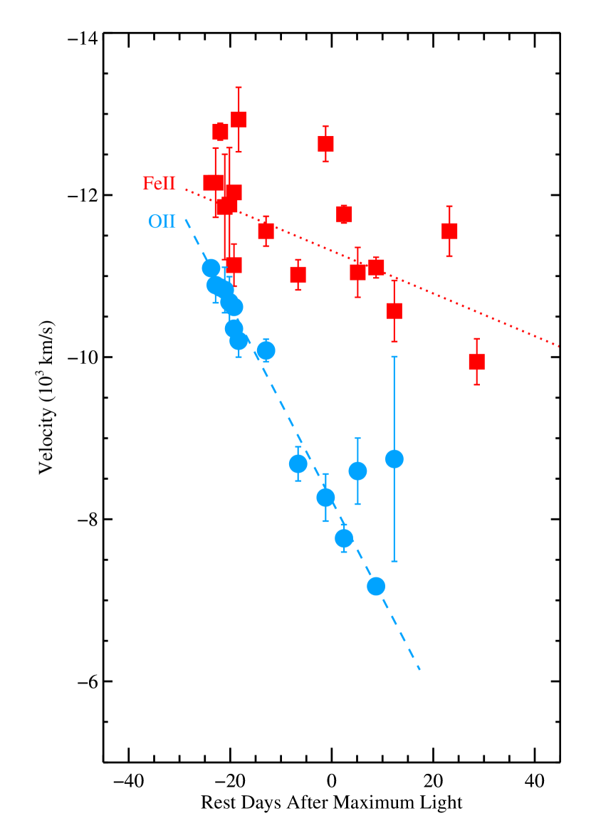
Figure 23: PTF12dam Fe II and O II line velocities as determined from cross-correlation against a spectrum with a reference velocity measured by fitting an absorption-line model to the data. Red squares show velocities from Fe II and blue circles indicate velocities from O II. The dotted and dashed lines show linear fits to the Fe II and O II line velocities, respectively.

In Figure 23 we compare the velocity evolution of the Fe II and O II ions in the spectra of PTF12dam. The O II velocities of PTF12dam are significantly ($\sim 1000$ km s^-1) slower than the Fe II velocities at the earliest phases, and they decline much more rapidly. The low velocities for O II imply that these lines form in lower levels of the ejecta, presumably closer to the photosphere than Fe II. Relatively high energies are required to coax oxygen into an ionized state where it may produce O II absorption (Mazzali et al., 2016), so these features may form closer to the main source of power than do the Fe II lines. Thus, the O II ion may better trace the photospheric velocities when they are the dominant spectral features.

8 Conclusions

We have shown that SLSNe-I are spectroscopically distinct from other types of SNe. Photospheric-phase spectra of SLSNe-I lack the strong hydrogen lines of SNe II, the strong Si II features characteristic of SNe Ia, and (usually) the strong He I features of SNe Ib. Under the classic classification scheme SLSNe-I could thus be considered SNe Ic, but this default category may encompass a wide variety of potentially physically distinct events. We do find, however, that there are spectroscopic differences between SLSNe-I and normal-luminosity SNe Ic that can be used to delineate these groups. SLSNe-I tend to have much bluer continua. To match SN Ic spectral templates to those of SLSNe-I, the templates typically need to be dereddened by $A_{V}\approx-2$ mag. Because normal-luminosity SNe Ic include events with a wide variety of spectral behaviors, we do not find a single feature that is always present in all SLSNe-I but never in normal-luminosity SNe Ic or vice versa. Rather, the spectroscopic distinction between SLSNe-I and SNe Ic at matching spectral phases, aside from continuum differences, is the combination of multiple minor differences. SLSNe-I tend to have weaker spectral features, and when a SLSN-I and a SN Ic are aligned in velocity space to one common feature, other features sometimes remain noticeably offset.

One obvious difference between SLSNe-I and SNe Ic is that O II features have never been observed in the spectra of the latter but are common in the early-time spectra of the former. Among all normal-luminosity SNe, only two peculiar events, the SN Ib SN 2008D (Soderberg et al., 2008; Mazzali et al., 2008; Modjaz et al., 2009) and the SN Ibn OGLE-2012-SN-006 (Pastorello et al., 2015), have shown these features. The long-lived presence of O II lines could be another defining feature of SLSNe-I, although there are several SLSNe-I that either did not show them or that were simply not observed at sufficiently early phases for these features to be seen (e.g., SN 2011ke). However, these SLSNe-I can still be separated from normal-luminosity SNe Ic by their later-phase spectra.

Aside from subtle differences, the spectral features of SLSNe-I around a month after maximum light are similar to those seen in SN Ic spectra near maximum light (Pastorello et al., 2010). Instead of comparing spectra of different SLSNe-I and SNe Ic to each other at the same light-curve phases, we study the differences in spectra at matched spectral phases. We define a spectral sequence using SLSNe-I which ranges from $\phi=-1$ for early-phase spectra with strong O II lines, to $\phi=0$ near the phase when these lines disappear, to $\phi=+1$ when the spectra resemble SNe Ic near maximum light, and finally to $\phi=+2$ when nebular emission lines begin to dominate. A given SN Ic or SLSN-I spectrum can be assigned a spectral phase by comparing the spectra to the ordered sequence shown in Figures 6–9 and identifying the closest match.

When comparing SLSN-I spectra to each other, we found that some objects had spectra similar to PTF12dam while other objects more closely resembled SN 2011ke. We compared the average spectra of these two groups and find that while the spectra are similar overall, there may be some systematic differences. SN 2011ke-like objects may exhibit smoother spectral features around $-0.3<\phi<+0.3$ than do PTF12dam-like objects. One interpretation of this is that the SN 2011ke-like objects have broader velocity distributions that tend to blend and smooth out individual ion features. This is supported by cross-correlation of SN 2011ke-like objects against the spectra of PTF12dam, which suggests higher expansion velocities for SN 2011ke-like objects. However, the systematic velocity shifts may only weakly correlate with feature width. For example, the SN 2011ke-like object PTF10bfz around $t=+18$ d is very similar to the spectra of SN 2011ke at $t\sim+25$ d, but the spectra of PTF10bfz have a systematic blueshift that is about 12,000 km s^-1 larger than that of SN 2011ke. Thus, the systematic velocity of PTF10bfz is much higher than for SN 2011ke, but the two objects appear to have similar velocity widths. We find a similar result for SN 2010gx, which is spectrally similar to PTF11rks at $\phi=-1$ but with a 6000 km s^-1 faster systematic blueshift.

Spectroscopic phases were defined under the assumption that the spectra of all SLSNe-I evolve in a consistent manner, but this may be undermined by the preference of some objects to better match either SN 2011ke or PTF12dam. In the full spectral sequence shown in Figures 6–9, it is evident that certain phases consist of spectra from one of these groups or the other. For example, in our spectral sequence the $1.11<\phi<1.46$ range has 21 SN 2011ke-like spectra but no PTF12dam-like spectra, and most of the spectra at $\phi<0$ (with strong O II lines) belong to the PTF12dam-like group. Perhaps we simply lack spectra of objects from the other groups at these phases (there are significant gaps in the temporal coverage of most SLSNe-I), but alternatively these groups may go through certain spectral phases that are not experienced by the other group (or only fleetingly experienced by the other group).

In addition to the O II lines, we find good evidence for C II, O I, Mg II, Si II, Ca II, Ti II, and Mn II in photospheric-phase spectra of SLSNe-I. Other ions likely contribute to the spectra as well, but these are difficult to securely identify using relatively primitive tools such as syn++. In particular, there is almost certainly Fe II $\lambda\lambda$4923, 5018, 5169 (other ions may contribute at these wavelengths as well), but syn++ predicts stronger Fe II features in the UV that conflict with the data. Non-LTE effects may need to be taken into account to properly model these features. The identification of the ions responsible for the four broad dips in the near-UV bands is similarly difficult to confirm with syn++. Previously suggested contributions from C III, Si III, Ti III, and Fe III remain plausible, but a simple comparison of the observed line minima against the predicted locations of these ions for a given blueshift leaves the true identities of these features in doubt. A complication to this picture is that these features likely evolve over time. This is especially apparent for the UV2 feature, which we find is most probably dominated by Mn II at late times but other ions at earlier phases. Far-UV spectra may hold the key to resoling these line identifications.

Even at similar spectral phases, the strengths of various features vary considerably among SLSNe-I. For example, PTF09cnd shows significantly stronger O II than PTF12dam around $\phi=-0.6$. Another example, LSQ12dlf, exhibits much larger peak-to-trough variations around $\phi=+1.25$ than does SN 2011ke. Our simple absorption-line modeling of the O II features between 3500 Å and 4800 Å (which blend into 5 dips that we label A–E from longest to shortest wavelength) provides a reasonably good fit to the spectra of PTF12dam and PTF09cnd considering it does not account for P-Cygni emission, but the models do not fare as well for SN 2010gx and PTF11rks. These objects have very weak O II C and D features and relatively strong E features around $\phi=-1$. When the models are fit to the O II B feature of PTF11rks, the predicted minima do not agree well with the data for the A, C, D, or E features. The culprit may be contamination from other lines as suggested by the slightly resolved A feature in PTF11rks.

As we have shown, it is difficult to measure accurate velocity curves in the spectra of SLSNe-I because the features are weak blends of more than one ion, and most features can only be detected over a limited range of phases. However, we have presented a method for measuring the velocity of the O II features, which are prominent in SLSN-I spectra up to around maximum light, by modeling them as simple Gaussian blends of multiplet lines. In doing so, we can determine a velocity matched to the absorption minima and a FWHM for the velocity distribution. The blueshift of the O II absorption minima in PTF12dam is measured through this technique to be about 11,000 km s^-1 in the earliest spectra and it has a FWHM of only 3000–4000 km s^-1. This relatively narrow velocity distribution supports the idea that O II is confined to a thin shell. The derived FWHM is sensitive to the assumed continuum level, but for PTF12dam the resolution of the O II B feature excludes velocity widths greater than $\sim 4000$ km s^-1. We also find that the O II absorption minima velocity of PTF12dam declines slowly by about 120 km s^-1 d^-1 (assuming a linear decay) by cross-correlating its spectra with a reference spectrum and noting the velocity shift. The O II velocities appear to be consistent with weak absorption features from C II, which we identify at both UV and optical wavelengths.

The subset of SLSNe-I with high systematic blueshifts (e.g., PTF10bfz) may result from particular viewing angles of highly asymmetric events, such as looking directly at jets of fast-moving material. Spectral polarimetry studies have begun to look for such geometries, and the implied asymmetries have thus far been low or similar to those of GRB-associated SNe Ic (Leloudas et al., 2015a; Inserra et al., 2016a). For some SLSNe-I, the velocities are not only lower but the velocity widths of the features are also very low. This is most readily evident in PTF12dam, for which the O II B is clearly resolved into two components at early phases, as discussed above. Thus, in contrast to Liu et al. (2016), we find at least some SLSNe-I have ion distributions that are rather narrow as compared to the broad spectral features that define SNe Ic-bl (but note that Liu et al. 2016 also find that the Fe II width of SN 2007bi is not only less than for SNe Ic-bl, it is less than the average SN Ic as well). We speculate that events like PTF10bfz may reflect the high-luminosity tail of the SN Ic-bl distribution, but events like PTF12dam that are far from broad lined may have an important physical difference. Late-time spectra of these events may help to determine if such SN 2011ke-like and PTF12dam-like events are physically distinct or if viewing-angle geometries are the deciding factor.

We show that there are other ions including Mg II and Fe II that appear to favor velocities higher than those of C II and O II. The velocities we measure for Fe II in the spectra of PTF12dam begin about 1000 km s^-1 faster and decline more slowly (only about 30 km s^-1 d^-1), although there is considerable scatter in the measurements. O II and C II may be better tracers of the photospheric velocity. If we assume spherical symmetry, then the presence of Mg II and Fe II at significantly higher velocities than the photosphere may disfavor the interaction model. This is because the photosphere would likely be located close to the fastest-moving ejecta, which are interacting with the slower-moving CSM, and this would leave little room for lines to form at higher velocities. Alternatively, we could be observing asymmetric explosion with jets of fast-moving Mg II and Fe II pointed at us. In this case we would predict that other events may have jets pointed away from the observer and thus lower apparent Mg II and Fe II velocities.

In the magnetar model the material is energized from within, in which case one might expect to see more highly ionized ions at later times. Metzger et al. (2014) suggest that some SLSNe-I may have an ionization front that moves out through the ejecta, eventually causing the ejecta to become transparent to X-rays. But this is not evident from the spectra in our SLSN-I sample. In particular, O II is only observed at early phases and O I strengthens at later phases. If these events are powered by magnetars, it would seem that the energy released by these central engines decreases substantially over time so that even as the ejecta expand and become less dense, the ionization front continues to recede with time.

Lacking adequate SLSN-II templates for our automated spectral classification, we have simply removed objects with obvious hydrogen emission consistent with SNe IIn from consideration as SLSNe-I. However, the relatively weak signs of hydrogen in the photospheric-phase spectra of PTF10aagc and otherwise plausible spectral similarities to SLSNe-I secured PTF10aagc a SLSN-I designation. This object is clearly distinct from others in the sample at least for its strong, broad H$\alpha$ at late phases. Similarly, our automated classification of PTF10hgi places it in the SLSN-I category as well (and this object has previously been published as a SLSN-I), but it is clearly distinct from other SLSNe-I in that it has clear signs of He I as well as hydrogen, suggesting a SLSN-IIb classification may be more appropriate. These outlying objects might favor a continuum between SLSNe-I and their hydrogen-rich SLSN-II cousins, but another possibility is that these are simply relatively high-luminosity examples of other, unrelated phenomena and we lack sufficient examples of each type to identify this division with our current tools.

Because the previously published SLSNe-I were based simply on peak luminosity and lack of obvious spectroscopic evidence for hydrogen, there may very well be objects in this group that meet these criteria but have physically different origins. This is one possible explanation for the preference of certain objects to have spectra more similar to those of either PTF12dam or SN 2011ke. We speculate that the PTF12dam-like objects with long-lived O II may form through one progenitor channel while more spectrally diffuse objects like PTF10bfz may represent the tail of the SN Ic-bl distribution. It may further be worth considering if PTF10hgi is a higher-luminosity relative of a SN 2005bf-like explosion, perhaps in the same family as the classic SN IIb SN 1993J.

Alternatively, some peculiar, lower-luminosity SNe may represent the low-luminosity tail of the SLSN-I/II distribution, and the longevity of O II features may be key to this connection. There have only been two lower-luminosity events, the SN Ib SN 2008D (Soderberg et al., 2008; Mazzali et al., 2008; Modjaz et al., 2009) and the SN Ibn OGLE-2012-SN-006 (Pastorello et al., 2015), that have shown these features. In both cases it has been argued that ejecta/CSM interactions are at play, and these may be important factors in maintaining the high temperatures (or at least the high levels of energy) required to ionize oxygen. Pastorello et al. (2015) favor CSM interaction as the dominant power source for OGLE-2012-SN-006, in which case oxygen must be either thermally excited or excited by hard radiation from the shocked material in order to explain the presence of O II. Mazzali et al. (2016) have argued that oxygen cannot be sufficiently excited thermally to produce the O II features in SLSNe-I and take these features as evidence of nonthermal excitation by a central magnetar. However, some studies of the bolometric light-curves of SLSNe-I favor power from CSM interaction (e.g., Wheeler et al. 2017; Tolstov et al. 2017b). Low-luminosity objects like OGLE-2012-SN-006 that have both clear signs of CSM interaction and strong O II spectroscopic features may make it worth considering what role such a process may play in the ionization state of SLSN-I envelopes.

The data presented here can further be used to help identify the underlying source of SLSN-I power and they may aid future studies of the possible connection between SNe Ic and SLSNe-I. Spectral properties such as the equivalent widths or velocities of particular features can be correlated with light-curve parameters such as peak luminosity, rise time, and fading rates. For example, we find that the time required for PTF12dam-like events to fade by 1 mag from maximum may be longer than for SN 2011ke-like events using the results of De Cia et al. (2017). The average fall time for seven PTF12dam-like events (PTF09atu, PTF09cnd, PTF10nmn, PTF10vqv, PTF11hrq, PTF12dam, and PTF12gty) is $54\pm 12$ d, whereas the average fall time for eight SN 2011ke-like events (PTF09as, PTF10aagc, PTF10bfz, 2010gx, PTF10hgi, PTF10uhf, 2011ke, and PTF11rks) is $24\pm 8$ d, with most of these later events clustered around fall times of 29 d. The $p$-value from a formal KS test is $3\times 10^{-4}$, which strongly rejects the null hypothesis that these two populations, divided by spectral properties, are drawn from the same light-curve distribution.

Our high-quality time-series spectra can be used to check predictions made by theoretical models regarding the velocity distribution and evolution of ejecta components. If a given model can naturally explain these observables for multiple SLSNe-I and for SNe Ic as well, then this might finally resolve the physical nature of these events. The limiting factor in this comparison may actually be a relative lack of SN Ic observations. There appears to be considerable diversity among so-called stripped-envelope SNe, and few have high-quality spectra extending into the rest-frame UV that can be compared against the higher-redshift SLSN-I sample. There could be multiple progenitor channels that lead to stellar explosions with relatively weak hydrogen, silicon, and helium in their spectra, so we may need to assemble a large sample of these objects with spectroscopic observations taken over a range of similar spectral phases and rest-wavelength ranges to properly compare and discriminate among them. Upcoming surveys, such as the Zwicky Transient Facility, will easily generate the requisite candidate pool for such work; the challenge will be to efficiently monitor these detections to generate new discoveries.

Appendix A Generalized Savitzky-Golay Smoothing of Spectra

SN spectra are often noisy and it is necessary to smooth them for use as comparison templates or simply for display purposes. The act of smoothing removes information from the data and should thus not be performed for some analyses. However, if most of the information lost is connected to noise, smoothing spectra can simplify the analysis. It is important, however, to maintain the integrity of the true signal. Because the spectral features of SNe are broadened by thousands of km s^-1, whereas most instruments sample the spectra in bins only tens of km s^-1 wide, it is relatively easy in most cases to isolate the signal from the bulk of the noise.

Standard techniques for smoothing spectra include the boxcar method, fast Fourier transform (FFT) filtering, and local polynomial fitting (e.g., Savitzky-Golay). In the boxcar method, the value in the $i^{\rm th}$ bin is replaced with the average of the values in bins $i-n$ to $i+n$. Boxcar smoothing is widely used because of its simplicity to implement, but it has the well-documented problem of washing out the true peaks and valleys of the signal. For FFT filtering, the spectrum is transformed to wave-number space, bins with wave numbers higher than expected for the broad SN features are muted, and the smoothed spectrum is recovered with application of a reverse FFT transform. FFT filtering often performs better than boxcar smoothing, but it requires the input spectra, which are usually sampled into bins with a constant wavelength width, $\delta\lambda$, to be resampled into bins of constant velocity width, $\delta v$. Any missing wavelength bins produced by gaps in coverage or rejection due to artifacts must first also be interpolated over. Thus, a nontrivial amount of preprocessing is required before the FFT filter can be applied. It is also not straightforward to account for measurement errors when FFT filtering a spectrum.

The standard Savitzky-Golay filter (Savitzky & Golay, 1964) is similar to the boxcar method in that the value in the $i^{\rm th}$ bin is replaced based on the values in bins $i-n$ to $i+n$, but instead of taking an average, a polynomial is fit to the chosen bins and the value of this polynomial in the $i^{\rm th}$ bin is reserved. The order of the polynomial fit can be varied to better fit faster variations in the input spectrum (if set to zero, boxcar smoothing is recovered). Thus, like the FFT method, Savitzky-Golay filtering can do a better job of preserving the signal. This filtering technique has many applications, including the smoothing of SN spectra (see, e.g., Silverman et al. 2012a).

When applied to SN spectra, we can generalize the Savitzky-Golay filtering technique to take advantage of the extra information available. Each spectral bin has not just one number but two or three: the wavelength, flux, and (often) the flux error values. Applying this additional information, we can naturally interpolate over missing data from bad pixels (e.g., cosmic-ray hits) and, to some extent, larger gaps caused by, for example, nonoverlapping two-channel observations. When the error spectrum is available, we can also use this to weight the fit. This can significantly improve the performance of the smoothing in regions subject to strong night-sky lines (with correspondingly large flux errors in limited bins).

As further generalization of the Savitzky-Golay filter, we can allow the number of bins included in the polynomial fitting to vary. This is desirable because most spectra are dispersed by gratings and thus have more bins per resolution element in the red as compared to the blue. Because the spectra are sampled in uniformly sized wavelength bins, SN features broadened by, say, 10,000 km s^-1 cover twice as many bins at 10,000 Å as compared to 5000 Å. We thus let the number of bins vary with wavelength to maintain constant sampling in velocity space.

Figure 24 shows the effects of smoothing on real data (with simulated noise). For each wavelength, $\lambda$, a second-order polynomial fit is performed to all data in the range $\lambda-\lambda/100<\lambda<\lambda+\lambda/100$. In order to facilitate comparison of the smoothed data to the original data, the smoothed data are output in identical wavelength bins; however, note that another advantage of this generalized Savitzky-Golay filtering is that the output wavelength scale need not match the input one exactly. We can thus in one step smooth and register spectra onto a desired wavelength scale. Similarly, the procedure can conveniently be used to stack a set of spectra even if they are each on shifted wavelength scales.

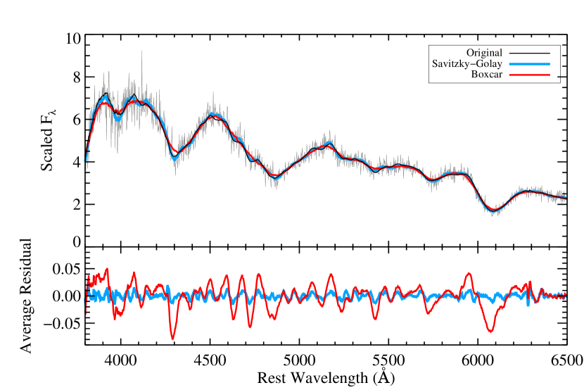
Figure 24: An example of generalized Savitzky-Golay and boxcar smoothing applied to spectra of a SN Ia. In the upper panel, the thick black line is a high-S/N ratio spectrum of SN 2011fe (Maguire et al., 2014). The thin gray line gives a realization of this spectrum with noise added. The thick red line shows the result of boxcar smoothing this latter, noisy spectrum, and the thicker blue line shows the result from generalized Savitzky-Golay filtering. In the lower panel we show the fractional difference between the original spectrum and the smoothed spectra averaged over 1000 realizations. It is apparent that the boxcar method performs poorly near the peaks and troughs of the spectral lines while the generalized Savitzky-Golay method handles these better.

Appendix B Spectral Template Matches to SNe Ic at $+30$d

Following the procedure detailed in §2, we have matched the spectra of three SNe Ic taken about one month after maximum light to our spectral template libraries. In Figure 25 we plot the best matching SN Ic, SN Ib, and SLSN-I to each of these spectra for comparison. Some later phase SLSN-I show many of the same spectral features as ordinary luminosity SNe Ic at this phase, but the SLSNe-I tend to have weaker features as perhaps best shown by the absorption dip near 5700 Å. SNe Ic and SNe Ib templates typically provide better matches during this phase according to the $\Delta I_{\rm Ic-X}$ scores.

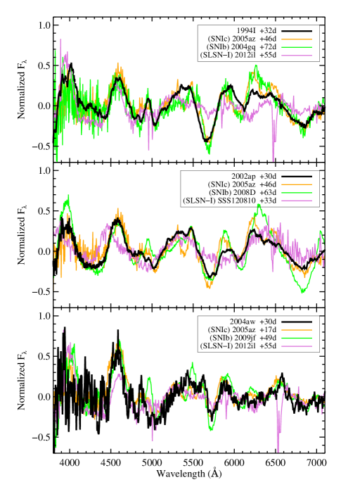
Figure 25: Best-fitting SN Ic, SN Ib, and SLSN-I spectral templates to the Type Ic supernovae SN 1994I, SN 2002ap, and SN 2004aw. The spectra and templates have been continuum divided and the templates have been shifted in velocity.

Appendix C Light-Curve Phase Estimates from Spectral Matching

Using our library of spectral templates taken at known light-curve phases we can test the precision and accuracy to which the light-curve phases of test spectra can be recovered. We use superfit to match the spectral templates to the input spectrum as described in §2 and then compare the actual light-curve phase of the input spectrum to the average light-curve phase of the top three matches of the correct type.

Figure 26 shows the actual phase of the SN Ia spectra tested vs. the average phase derived from the best superfit matches. We find that the averaged superfit phases are typically biased by less than 0.5 d (with superfit preferring slightly later phases) between about 1 week before maximum light to about 1 month after. Over this period the standard deviation is around 2.3 d with measurements closer to maximum light faring better. This result is similar to that of Riess et al. (1997), who find a precision of 1.4 d over a comparable range of phases, and Blondin et al. (2012), who find a 2.9 d dispersion in spectral ages for SNe Ia within about 10 days of maximum light. We find that the accuracy remains good to at least two months after maximum light but the standard deviation degrades to about 5 d.

We also tested the precision and accuracy of SN Ic and SLSN-I phases derived from spectral template matching. The median absolute bias is 2.2 d for the SN Ic sample and 8.0 d for the SLSNe-I. The standard deviations of the difference between the actual light-curve phases and the averaged values of the best superfit matches are also significantly higher for the SNe Ic and SLSNe-I than for the SN Ia sample. For SNe Ic the standard deviation rises from about 6 d one week before maximum light to about 17 d one month after maximum. The standard deviations of the SLSN-I sample are about 15 d over a similar time period. These larger values could reflect the smaller sample sizes or greater intrinsic differences in the spectra and how these vary with light-curve phase.

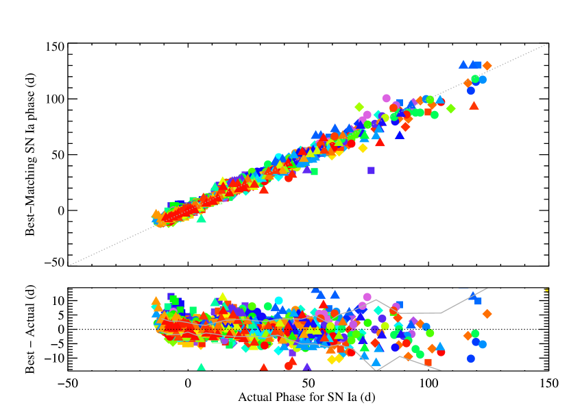
Figure 26: Precision and accuracy of SN Ia light-curve phases derived from spectral template matching. The top panel plots the real phase against the derived phase and the lower panel shows the residual from the true values. The gray lines show the $1\sigma$ range of the residuals evaluated in several phase bins. All spectra for a given object are plotted with the same color, and a different color is used for each object. Marker shapes reflect the subtype of the SN Ia: triangles for SN Ia-SS, squares for SN Ia-CL, diamonds for SN Ia-BL, and circles for SN Ia-CN.

Appendix D On the He I $\lambda 10830$ Line in SN 2012il

To investigate the reported discovery of helium in the spectra of SN 2012il by Inserra et al. (2013), we downloaded the 2012 March 17 VLT+XSHOOTER spectra of this object. In studying the spectra we found that the data agree well with what is plotted in the main part of Figure 9 from Inserra et al. (2013), but we do not reproduce the results from the right panel of this figure, which is intended to show a smoothed version of the reported He I $\lambda 10830$ line. Instead, we find that there is a broad emission bump in this region, but it is significantly offset to the red of 10,830 Å by about 1500 km s^-1. In Figure 27 we show the data in this region without applying any smoothing. As can be seen, there are narrow emission lines at 10,830 Å and 10,938 Å, which are likely He I and hydrogen Pa-$\gamma$ from the host galaxy. The broad emission bump is centered in between these. The detection of the narrow host lines shows that the wavelength solution is accurate and that the broad bump is thus not centered at 10,830 Å as was reported. Given the offset, we find it unlikely that this feature is associated with helium. An association with hydrogen may be possible (nebular hydrogen lines are sometimes blueshifted owing to geometric effects; e.g., Yan et al. 2015), but in this case the lack of hydrogen Balmer lines in the spectra is puzzling.

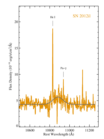
Figure 27: Near-infrared spectra of SN 2012il highlighting the He I $\lambda 10830$ region. Data are from Inserra et al. (2013). The gray curve shows a Gaussian function fit to the data. The Gaussian is centered at 10,883 Å, which is redshifted by about 1500 km s^-1 from the expected position of the He I line. Narrow emission lines matching the wavelengths of He I $\lambda 10830$ and hydrogen Pa-$\gamma$ in the host-galaxy frame are labeled.

Appendix E Spectra of PTF SLSN-I

In Figures 28–38 we plot the 166 spectra of likely and possible SLSNe-I recorded by the PTF survey. Included are 34 spectra previously published for SN 2010gx, SN 2011ke, PTF10hgi, PTF11rks, and PTF12dam (Pastorello et al., 2010; Quimby et al., 2011; Nicholl et al., 2013; Inserra et al., 2013). Each extracted spectrum has been processed to remove narrow emission lines from the host environment. Similar to the discussion in §2, lines are removed by simultaneously fitting Gaussians at the expected wavelengths of host-galaxy lines, with all lines in a given fit required to have the same width. The fitting is done section by section (e.g., lines near H$\alpha$, then H$\beta$, etc.). We shift the spectra to the host-galaxy rest frame and vertically for clarity, and we overplot a smoothed version of the spectra (see §A). Each spectrum is labeled with the object name and light-curve phase. Other than the narrow emission lines, host-galaxy light has not been removed from these spectra, and this may dominate the signal at later phases in some cases.

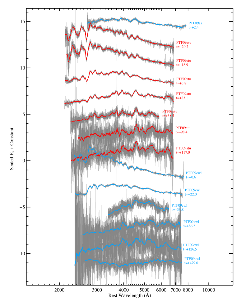
Figure 28: Spectra of PTF09as, PTF09atu, and PTF09cwl.

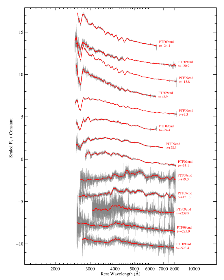
Figure 29: Spectra of PTF09cnd.

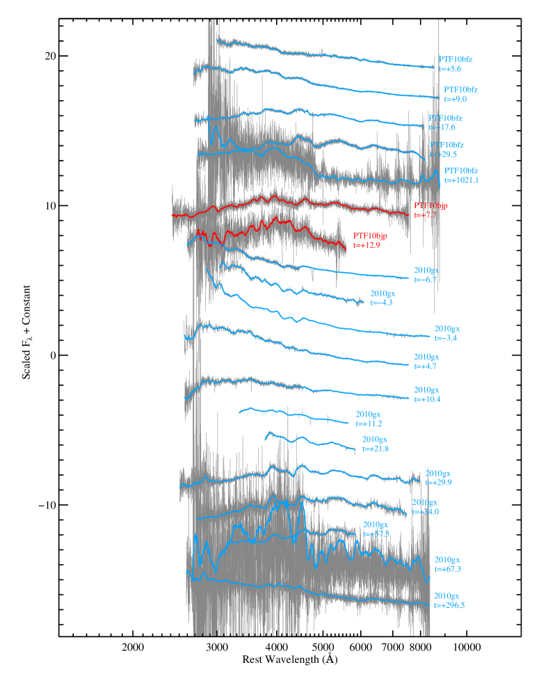
Figure 30: Spectra of PTF10bfz, PTF10bjp, and SN 2010gx.

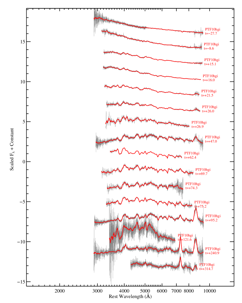
Figure 31: Spectra of PTF10hgi.

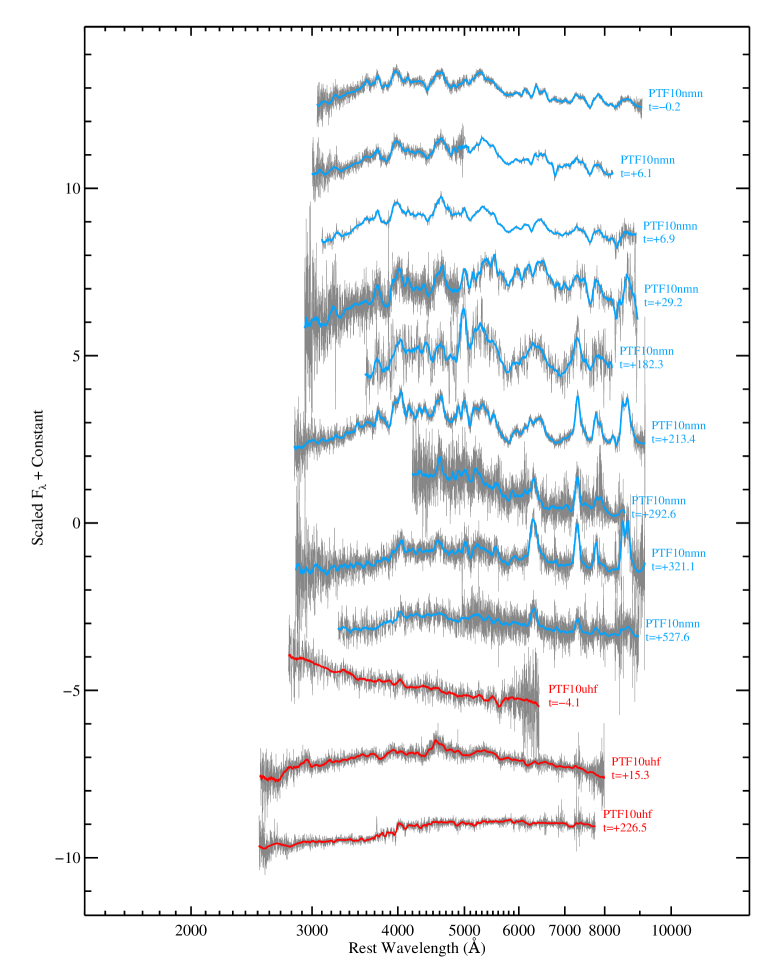
Figure 32: Spectra of PTF10nmn and PTF10uhf.

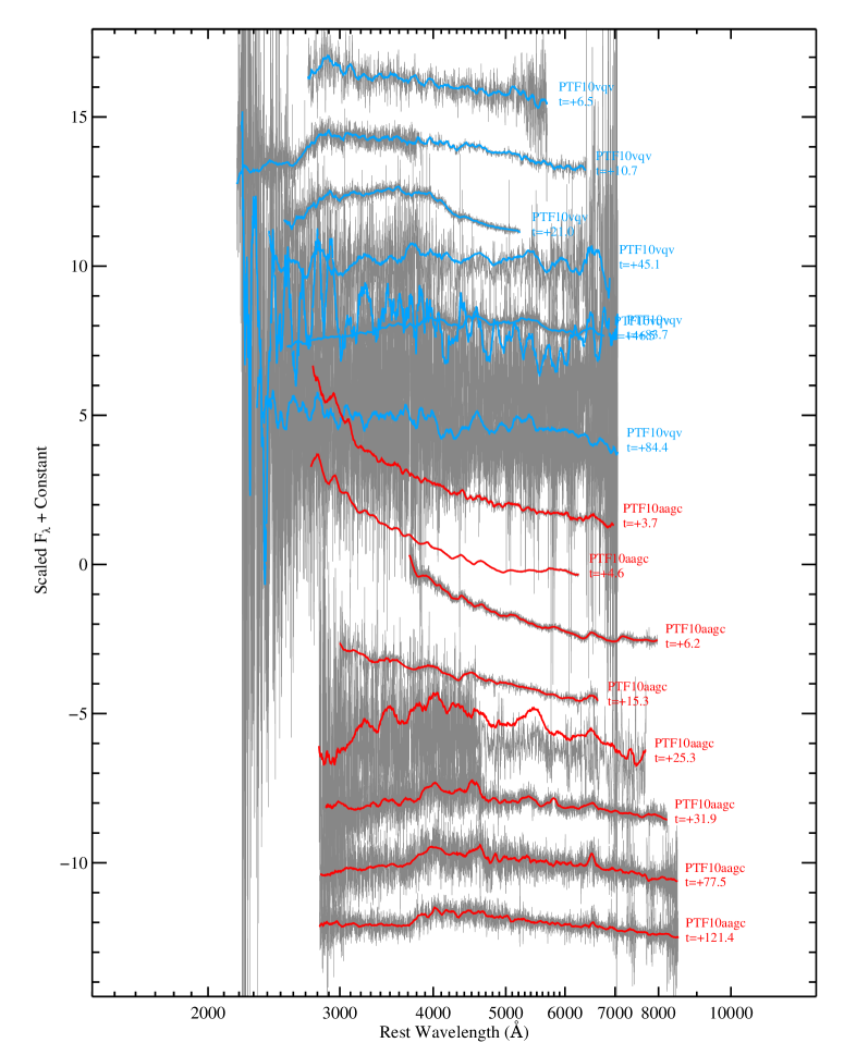
Figure 33: Spectra of PTF10vqv and PTF10aagc.

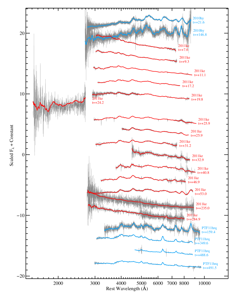
Figure 34: Spectra of SN 2010hy, SN 2011ke, and PTF11hrq.

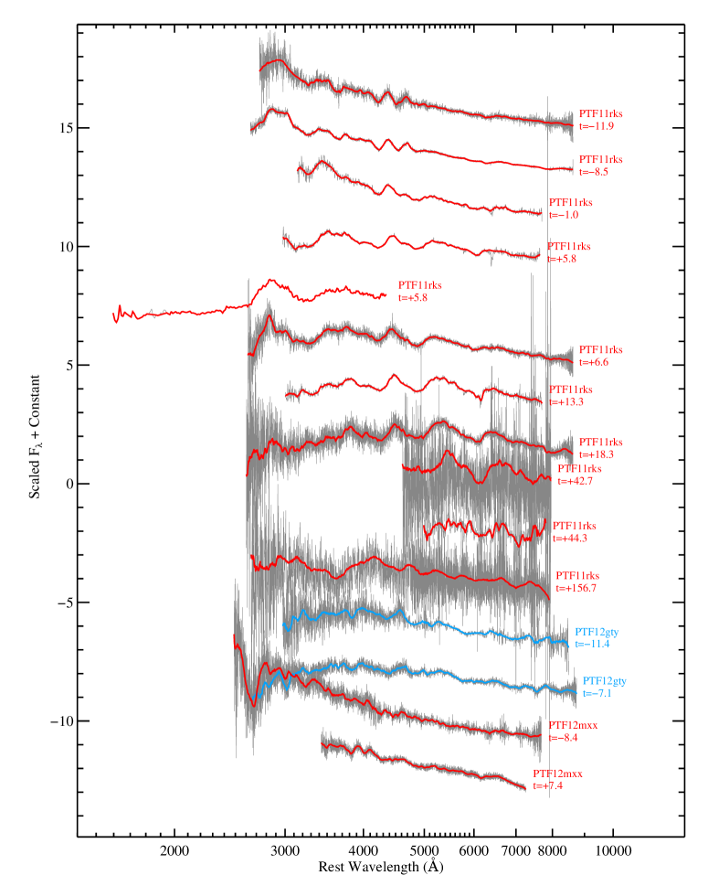
Figure 35: Spectra of PTF11rks, PTF12gty, and PTF12mxx.

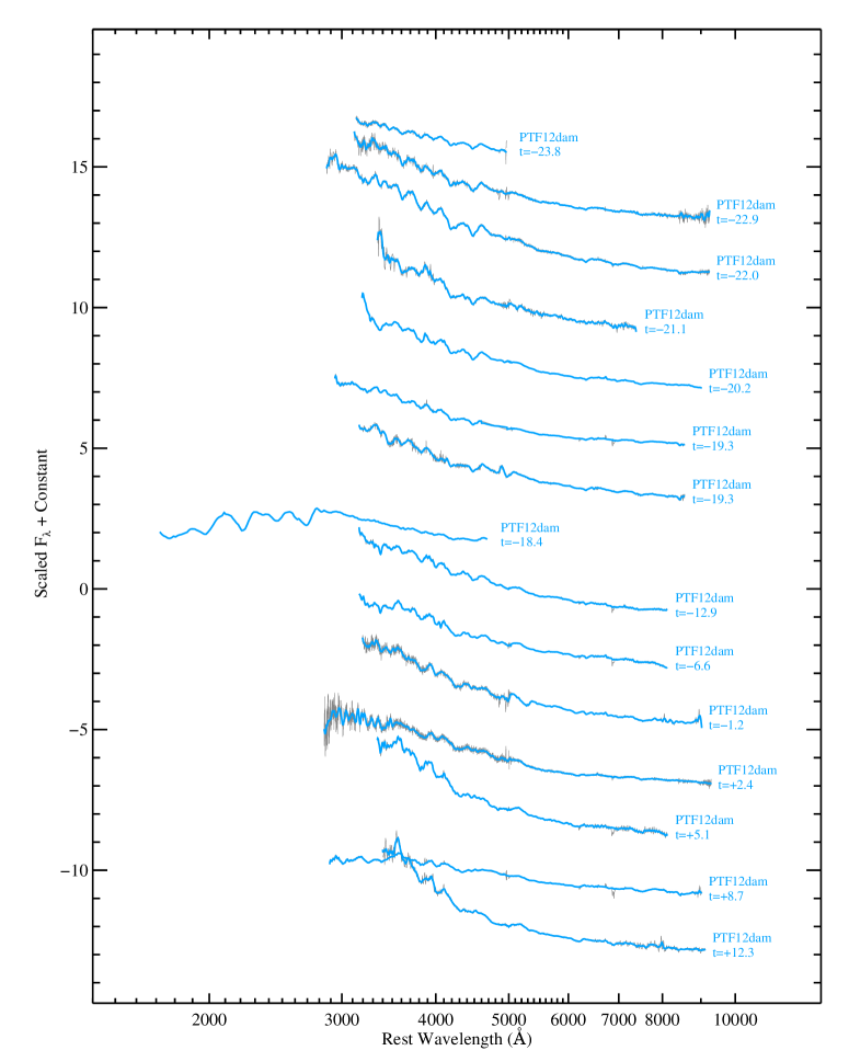
Figure 36: Spectra of PTF12dam from $t=-25.3$ through $t=+10.8$ d.

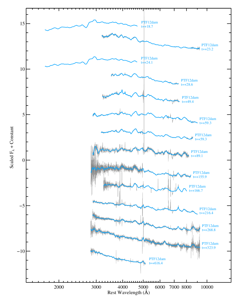
Figure 37: Spectra of PTF12dam from $t=+17.2$ through $t=+614.9$ d.

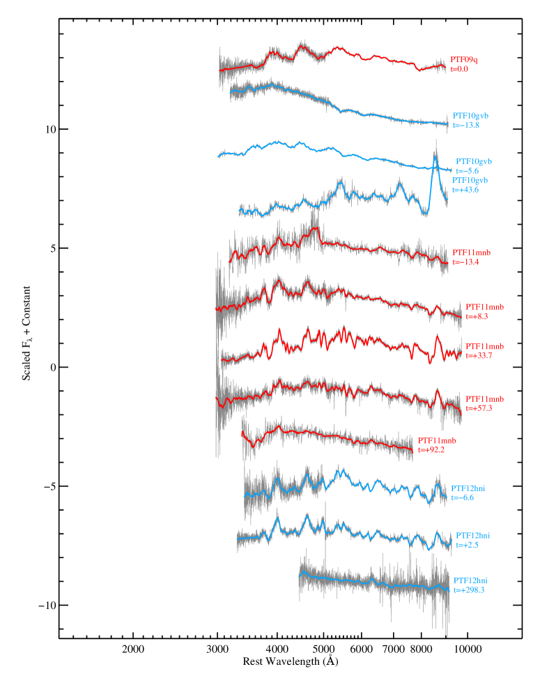
Figure 38: Spectra of the possible SLSNe-I PTF09q, PTF10gvb, PTF11mnb, and PTF12hni.

Appendix F Average Spectral Features at $\phi\approx-1.0$

In Figure 39 we show the average spectrum of SLSNe-I at early phases ($-1.5<\phi<-0.5$) constructed as described in §5. A syn++ model was constructed using ions previously associated with SNe, especially SLSNe-I. For all ion species we adopt the same velocity distributions to eliminate some degree of freedom. We essentially fit only for the strength of the ion and retain only those ions which appear to contribute significantly to the average observed spectrum while not introducing superfluous features into the model. We adopt an ion temperature of 10,000 K for the models, except for the oxygen lines for which 15,000 K seems to produce better results.

The strongest features in the average spectrum —-three broad dips in the range 2100–2800 Å — can be reasonably well fit by blends of C II, C III, Si III, Ti III, and Mg II (Dessart et al., 2012; Howell et al., 2013; Mazzali et al., 2016). A weak, broad dip at 2900–3300 Å can be explained by Ti II with a minor contribution from O II (a check using syn++ found no other obvious ion species that could explain this dip without introducing other, stronger features that conflict with the data). The strongest features in the optical range — two dips in the range 4000–4700 Å —a re well fit by O II (Quimby et al., 2011). As previously found, O II is also the main contributor to other, weaker dips to the blue of this “W” feature. However, the syn++ model significantly overpredicts the absorption around 3900 Å. This discrepancy is investigated further in §6.1. Note we do not include Ca II at this phase, as it does not improve the quality of the fit. However, at later phases this ion may become dominate around 3800 Å. The O II features may also be blended with C II and possibly Si II. The latter ion is typically invoked to explain a common feature at 6150 Å in SN spectra. For SLSNe-I, this feature may be blended with C II. If Si II is present, then syn++ predicts there should be stronger lines in the UV around 1450 Å and 1720 Å as well. In addition to the C II lines near 6300 Å and 6940 Å (Quimby et al., 2011; Yan et al., 2017a), there are likely features from O I including the triplet around 7774 Å (Nicholl et al., 2016).

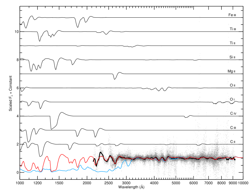
Figure 39: Synthetic spectral model (red) from syn++ compared to the average of SLSN-I spectra in the range $-1.5<\phi<-0.5$ (thick black line). The spectra have been continuum divided to emphasize the features. Gray points show contributions to the average spectrum from individual object spectra. Contributions to the syn++ fit from each individual ion are plotted with thin black lines and shifted vertically for clarity. The blue curve shows the effect of adding Fe II to the model. The absorption near 4900 Å, can be well fit with this change, but in doing so the syn++ models predict a strong feature at about 3050 Å and severe line blanketing below 3000 Å, which is not observed.

Appendix G Average Spectral Features at $\phi\approx 0$

In Figure 40 we show the average SLSN-I spectrum in the $-0.5<\phi<+0.5$ range. The syn++ fit includes many of the same ions as in the earlier-phase spectra, but some of these have been adjusted in strength. In particular, the O II features may persist to this phase, but they appear weaker and are more noticeably blended with other ions. Ca II may be weakly detected at this phase, and Mg II may start to dominate near 4300 Å. A predicted Mg II feature near 8900 Å, possibly blended with O II, is not well matched to the data. There is a weak, broad dip near 4850 Å that can be well fit by Fe II; however, to match this feature’s strength syn++ predicts a strong feature at 3050 Å and severe line blanketing at shorter wavelengths, which is not observed. Following numerical modeling of other SNe, most likely the 4850 Å feature is a blend of Fe II. The poor syn++ match to the UV portion of the spectrum could presumably be due to non-LTE effects, but investigation of this discrepancy is left to future works. It is also notable that while the strong features in the UV near 1950 Å and 2650 Å are well matched by the syn++ model, the positions of the minima for the 2200 Å and 2400 Å features are systematically offset. This could indicate incorrect line identifications, which is investigated further in §6.

We also note that the observations suggest a weak absorption feature near 5500 Å. Using syn++ to check possible ion species we find few options for its production without the addition of stronger features as well in the wavelength range constrained by our spectral sample. One possibility shown in Figure 40 is that this absorption is caused by C IV. If this identification is correct, then syn++ predicts that a much stronger line should also form at $\sim 1400$ Å. Recent, rest-frame far-UV observations of the SLSN-I Gaia16apd have revealed a strong feature near this wavelength (Yan et al., 2017a), which may match the one predicted by syn++. Detailed modeling is required to test the validity of this tentative assignment.

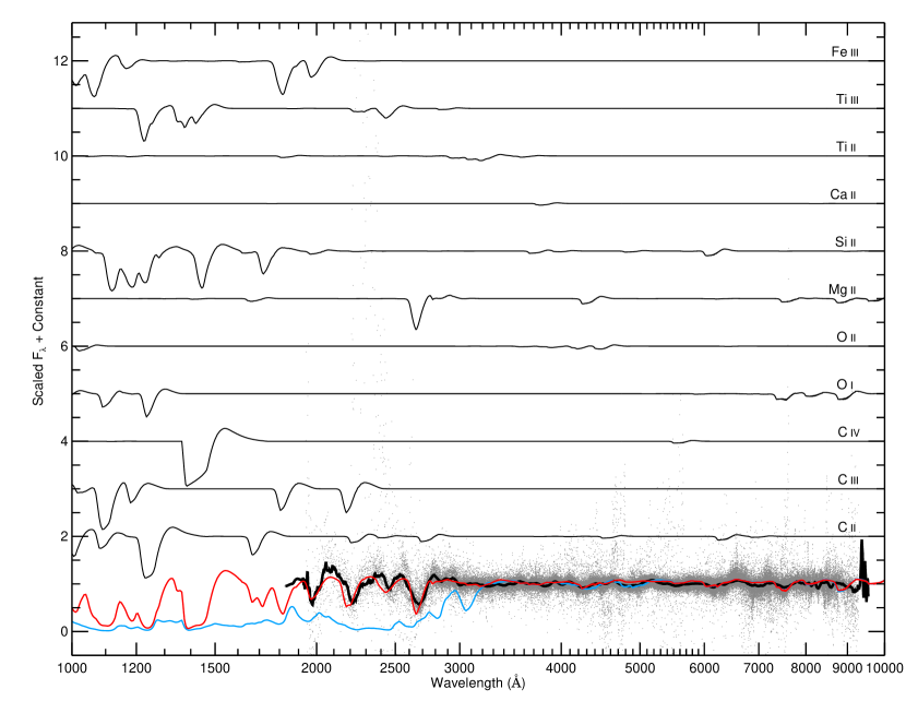
Figure 40: Similar to Figure 39 but for the average SLSN-I spectrum in the $-0.5<\phi<+0.5$ range.

Appendix H Average Spectral Features at $\phi\approx+1.0$

In Figure 41 we show the average SLSN-I spectrum in the $+0.5<\phi<+1.5$ range with a syn++ model. To fit the 2000 Å absorption feature with Fe III as has previously been suggested (Howell et al., 2013) syn++ predicts a stronger feature at 1850 Å that conflicts with the data. Again, the inclusion of Fe II in the fit greatly improves the agreement in the optical portion of the spectrum near 4800 Å and also near 4100 Å; however, the model differs significantly from the average observed spectrum in the UV. This includes a strong predicted feature around 3050 Å and near total absorption around 2400 Å. We do note, however, some rough agreement between peaks in the model flux (including Fe II) in the range 1700–2200 Å. Thus, it is possible that Fe II does contribute significantly to the UV portion of the spectrum at this phase. Some of the discrepancy between the data and the model including Fe II in Figure 41 may be due to the way the observational data were continuum divided, but this would not explain the 3050 Å feature nor the relatively high luminosity observed in the UV bands.

The model fit indicates the O II lines have subsided and that the dominant features in the optical range are now from Mg II, Fe II, and Ca II. Moving to the near-infrared, there is O I, which produces three dips at 7500 Å, 8100 Å, and 8900 Å. The Mg II also has relatively strong features in this range which may contribute to these dips. A further contributor may be Fe II, although the strengths of its lines are uncertain from the non-LTE syn++ models as noted above.

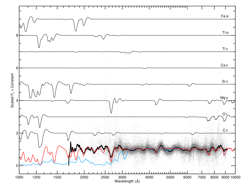
Figure 41: Similar to Figures 39 and 40 but for the average SLSN-I spectrum in the $+0.5<\phi<+1.5$ range.

References

- Arcavi et al. (2010) Arcavi, I., Gal-Yam, A., Kasliwal, M. M., et al. 2010, ApJ, 721, 777
- Barbary et al. (2009) Barbary, K., Dawson, K. S., Tokita, K., et al. 2009, ApJ, 690, 1358
- Barbon et al. (1995) Barbon, R., Benetti, S., Cappellaro, E., et al. 1995, A&AS, 110, 513
- Barkat et al. (1967) Barkat, Z., Rakavy, G., & Sack, N. 1967, Physical Review Letters, 18, 379
- Bayless et al. (2013) Bayless, A. J., Pritchard, T. A., Roming, P. W. A., et al. 2013, ApJ, 764, L13
- Benetti et al. (2014) Benetti, S., Nicholl, M., Cappellaro, E., et al. 2014, MNRAS, 441, 289
- Berger et al. (2012) Berger, E., Chornock, R., Lunnan, R., et al. 2012, ApJ, 755, L29
- Blondin & Tonry (2007) Blondin, S., & Tonry, J. L. 2007, ApJ, 666, 1024
- Blondin et al. (2012) Blondin, S., Matheson, T., Kirshner, R. P., et al. 2012, AJ, 143, 126
- Bose et al. (2017) Bose, S., Dong, S., Pastorello, A., et al. 2017, ArXiv e-prints, arXiv:1708.00864
- Branch et al. (2002) Branch, D., Benetti, S., Kasen, D., et al. 2002, ApJ, 566, 1005
- Branch et al. (2008) Branch, D., Jeffery, D. J., Parrent, J., et al. 2008, PASP, 120, 135
- Bufano et al. (2009) Bufano, F., Immler, S., Turatto, M., et al. 2009, ApJ, 700, 1456
- Cardelli et al. (1989) Cardelli, J. A., Clayton, G. C., & Mathis, J. S. 1989, ApJ, 345, 245
- Chatzopoulos & Wheeler (2012) Chatzopoulos, E., & Wheeler, J. C. 2012, ApJ, 748, 42
- Chatzopoulos et al. (2013) Chatzopoulos, E., Wheeler, J. C., Vinko, J., Horvath, Z. L., & Nagy, A. 2013, ApJ, 773, 76
- Chatzopoulos et al. (2011) Chatzopoulos, E., Wheeler, J. C., Vinko, J., et al. 2011, ApJ, 729, 143
- Chen et al. (2013) Chen, T.-W., Smartt, S. J., Bresolin, F., et al. 2013, ApJ, 763, L28
- Chen et al. (2017) Chen, T.-W., Nicholl, M., Smartt, S. J., et al. 2017, A&A, 602, A9
- Chevalier & Irwin (2011) Chevalier, R. A., & Irwin, C. M. 2011, ApJ, 729, L6
- Chomiuk et al. (2011) Chomiuk, L., Chornock, R., Soderberg, A. M., et al. 2011, ApJ, 743, 114
- Chornock et al. (2013) Chornock, R., Berger, E., Rest, A., et al. 2013, ApJ, 767, 162
- Cikota et al. (2017) Cikota, A., De Cia, A., Schulze, S., et al. 2017, MNRAS, 469, 4705
- Crowther et al. (2016) Crowther, P. A., Caballero-Nieves, S. M., Bostroem, K. A., et al. 2016, MNRAS, 458, 624
- Dall’Ora et al. (2014) Dall’Ora, M., Botticella, M. T., Pumo, M. L., et al. 2014, ApJ, 787, 139
- De Cia et al. (2017) De Cia, A., Gal-Yam, A., Rubin, A., et al. 2017, ArXiv e-prints, arXiv:1708.01623
- Dessart & Hillier (2005) Dessart, L., & Hillier, D. J. 2005, A&A, 439, 671
- Dessart et al. (2012) Dessart, L., Hillier, D. J., Waldman, R., Livne, E., & Blondin, S. 2012, MNRAS, 426, L76
- Drake et al. (2009a) Drake, A. J., Mahabal, A. A., Djorgovski, S. G., et al. 2009a, The Astronomer’s Telegram, 1980
- Drake et al. (2009b) Drake, A. J., Mahabal, A., Djorgovski, S. G., et al. 2009b, Central Bureau Electronic Telegrams, 1752
- Fabricant et al. (1998) Fabricant, D., Cheimets, P., Caldwell, N., & Geary, J. 1998, PASP, 110, 79
- Fassia et al. (2001) Fassia, A., Meikle, W. P. S., Chugai, N., et al. 2001, MNRAS, 325, 907
- Filippenko (1982) Filippenko, A. V. 1982, PASP, 94, 715
- Filippenko (1997) —. 1997, ARA&A, 35, 309
- Filippenko et al. (2001) Filippenko, A. V., Li, W. D., Treffers, R. R., & Modjaz, M. 2001, in Astronomical Society of the Pacific Conference Series, Vol. 246, IAU Colloq. 183: Small Telescope Astronomy on Global Scales, ed. B. Paczynski, W.-P. Chen, & C. Lemme, 121
- Filippenko et al. (1992) Filippenko, A. V., Richmond, M. W., Branch, D., et al. 1992, AJ, 104, 1543
- Filippenko et al. (1995) Filippenko, A. V., Barth, A. J., Matheson, T., et al. 1995, ApJ, 450, L11
- Folatelli et al. (2006) Folatelli, G., Contreras, C., Phillips, M. M., et al. 2006, ApJ, 641, 1039
- Foley et al. (2003) Foley, R. J., Papenkova, M. S., Swift, B. J., et al. 2003, PASP, 115, 1220
- Fowler & Hoyle (1964) Fowler, W. A., & Hoyle, F. 1964, ApJS, 9, 201
- Fransson et al. (1996) Fransson, C., Lundqvist, P., & Chevalier, R. A. 1996, ApJ, 461, 993
- Fransson et al. (2005) Fransson, C., Challis, P. M., Chevalier, R. A., et al. 2005, ApJ, 622, 991
- Gal-Yam (2012) Gal-Yam, A. 2012, Science, 337, 927
- Gal-Yam (2016) —. 2016, ArXiv e-prints, arXiv:1611.09353
- Gal-Yam et al. (2009) Gal-Yam, A., Mazzali, P., Ofek, E. O., et al. 2009, Nature, 462, 624
- Gal-Yam et al. (2011) Gal-Yam, A., Kasliwal, M. M., Arcavi, I., et al. 2011, ApJ, 736, 159
- Gezari et al. (2009) Gezari, S., Halpern, J. P., Grupe, D., et al. 2009, ApJ, 690, 1313
- González-Gaitán et al. (2011) González-Gaitán, S., Perrett, K., Sullivan, M., et al. 2011, ApJ, 727, 107
- Guillochon et al. (2017) Guillochon, J., Parrent, J., Kelley, L. Z., & Margutti, R. 2017, ApJ, 835, 64
- Harutyunyan et al. (2008) Harutyunyan, A. H., Pfahler, P., Pastorello, A., et al. 2008, A&A, 488, 383
- Hatano et al. (2001) Hatano, K., Branch, D., Nomoto, K., et al. 2001, in Bulletin of the American Astronomical Society, Vol. 33, American Astronomical Society Meeting Abstracts #198, 838
- Howell et al. (2006) Howell, D. A., Sullivan, M., Nugent, P. E., et al. 2006, Nature, 443, 308
- Howell et al. (2013) Howell, D. A., Kasen, D., Lidman, C., et al. 2013, ApJ, 779, 98
- Inserra et al. (2016a) Inserra, C., Bulla, M., Sim, S. A., & Smartt, S. J. 2016a, ApJ, 831, 79
- Inserra & Smartt (2014) Inserra, C., & Smartt, S. J. 2014, ApJ, 796, 87
- Inserra et al. (2013) Inserra, C., Smartt, S. J., Jerkstrand, A., et al. 2013, ApJ, 770, 128
- Inserra et al. (2016b) Inserra, C., Smartt, S. J., Gall, E. E. E., et al. 2016b, ArXiv e-prints, arXiv:1604.01226
- Jeffery & Branch (1990) Jeffery, D. J., & Branch, D. 1990, in Supernovae, Jerusalem Winter School for Theoretical Physics, ed. J. C. Wheeler, T. Piran, & S. Weinberg, 149
- Jerkstrand et al. (2014) Jerkstrand, A., Smartt, S. J., Fraser, M., et al. 2014, MNRAS, 439, 3694
- Jerkstrand et al. (2017) Jerkstrand, A., Smartt, S. J., Inserra, C., et al. 2017, ApJ, 835, 13
- Kasen & Bildsten (2010) Kasen, D., & Bildsten, L. 2010, ApJ, 717, 245
- Kasliwal et al. (2009a) Kasliwal, M. M., Quimby, R., Nugent, P., et al. 2009a, The Astronomer’s Telegram, 1983
- Kasliwal et al. (2009b) —. 2009b, Central Bureau Electronic Telegrams, 1732
- Kelson (2003) Kelson, D. D. 2003, PASP, 115, 688
- Kodros et al. (2010) Kodros, J., Cenko, S. B., Li, W., et al. 2010, Central Bureau Electronic Telegrams, 2461
- Kozyreva et al. (2017) Kozyreva, A., Gilmer, M., Hirschi, R., et al. 2017, MNRAS, 464, 2854
- Kümmel et al. (2009) Kümmel, M., Walsh, J. R., Pirzkal, N., Kuntschner, H., & Pasquali, A. 2009, PASP, 121, 59
- Law et al. (2009) Law, N. M., Kulkarni, S. R., Dekany, R. G., et al. 2009, PASP, 121, 1395
- Leloudas et al. (2012) Leloudas, G., Chatzopoulos, E., Dilday, B., et al. 2012, A&A, 541, A129
- Leloudas et al. (2015a) Leloudas, G., Patat, F., Maund, J. R., et al. 2015a, ApJ, 815, L10
- Leloudas et al. (2015b) Leloudas, G., Schulze, S., Krühler, T., et al. 2015b, MNRAS, 449, 917
- Leonard et al. (2000) Leonard, D. C., Filippenko, A. V., Barth, A. J., & Matheson, T. 2000, ApJ, 536, 239
- Leonard et al. (2002) Leonard, D. C., Filippenko, A. V., Li, W., et al. 2002, AJ, 124, 2490
- Li et al. (2011) Li, W., Leaman, J., Chornock, R., et al. 2011, MNRAS, 412, 1441
- Liu et al. (2017) Liu, L.-D., Wang, S.-Q., Wang, L.-J., et al. 2017, ApJ, 842, 26
- Liu et al. (2016) Liu, Y.-Q., Modjaz, M., & Bianco, F. B. 2016, ArXiv e-prints, arXiv:1612.07321
- Lunnan et al. (2016) Lunnan, R., Chornock, R., Berger, E., et al. 2016, ApJ, 831, 144
- Lunnan et al. (2017) —. 2017, ArXiv e-prints, arXiv:1708.01619
- Maguire et al. (2014) Maguire, K., Sullivan, M., Pan, Y.-C., et al. 2014, MNRAS, 444, 3258
- Malesani et al. (2009) Malesani, D., Fynbo, J. P. U., Hjorth, J., et al. 2009, in American Institute of Physics Conference Series, Vol. 1111, American Institute of Physics Conference Series, ed. G. Giobbi, A. Tornambe, G. Raimondo, M. Limongi, L. A. Antonelli, N. Menci, & E. Brocato, 627–628
- Marion et al. (2009) Marion, G. H., Höflich, P., Gerardy, C. L., et al. 2009, AJ, 138, 727
- Matheson et al. (2001) Matheson, T., Filippenko, A. V., Li, W., Leonard, D. C., & Shields, J. C. 2001, AJ, 121, 1648
- Mazzali et al. (2016) Mazzali, P. A., Sullivan, M., Pian, E., Greiner, J., & Kann, D. A. 2016, MNRAS, 458, 3455
- Mazzali et al. (2008) Mazzali, P. A., Valenti, S., Della Valle, M., et al. 2008, Science, 321, 1185
- Metzger et al. (2014) Metzger, B. D., Vurm, I., Hascoët, R., & Beloborodov, A. M. 2014, MNRAS, 437, 703
- Miller et al. (2009) Miller, A. A., Chornock, R., Perley, D. A., et al. 2009, ApJ, 690, 1303
- Modjaz et al. (2009) Modjaz, M., Li, W., Butler, N., et al. 2009, ApJ, 702, 226
- Modjaz et al. (2014) Modjaz, M., Blondin, S., Kirshner, R. P., et al. 2014, AJ, 147, 99
- Nicholl et al. (2017a) Nicholl, M., Berger, E., Margutti, R., et al. 2017a, ApJ, 845, L8
- Nicholl et al. (2017b) Nicholl, M., Guillochon, J., & Berger, E. 2017b, ArXiv e-prints, arXiv:1706.00825
- Nicholl et al. (2013) Nicholl, M., Smartt, S. J., Jerkstrand, A., et al. 2013, Nature, 502, 346
- Nicholl et al. (2014) —. 2014, MNRAS, 444, 2096
- Nicholl et al. (2015) —. 2015, MNRAS, 452, 3869
- Nicholl et al. (2016) Nicholl, M., Berger, E., Smartt, S. J., et al. 2016, ApJ, 826, 39
- Pastorello et al. (2004) Pastorello, A., Zampieri, L., Turatto, M., et al. 2004, MNRAS, 347, 74
- Pastorello et al. (2006) Pastorello, A., Sauer, D., Taubenberger, S., et al. 2006, MNRAS, 370, 1752
- Pastorello et al. (2007) Pastorello, A., Smartt, S. J., Mattila, S., et al. 2007, Nature, 447, 829
- Pastorello et al. (2008) Pastorello, A., Quimby, R. M., Smartt, S. J., et al. 2008, MNRAS, 389, 131
- Pastorello et al. (2009) Pastorello, A., Valenti, S., Zampieri, L., et al. 2009, MNRAS, 394, 2266
- Pastorello et al. (2010) Pastorello, A., Smartt, S. J., Botticella, M. T., et al. 2010, ApJ, 724, L16
- Pastorello et al. (2015) Pastorello, A., Wyrzykowski, Ł., Valenti, S., et al. 2015, MNRAS, 449, 1941
- Patat et al. (2001) Patat, F., Cappellaro, E., Danziger, J., et al. 2001, ApJ, 555, 900
- Perley et al. (2016) Perley, D. A., Quimby, R. M., Yan, L., et al. 2016, ApJ, 830, 13
- Prajs et al. (2017) Prajs, S., Sullivan, M., Smith, M., et al. 2017, MNRAS, 464, 3568
- Prentice et al. (2016) Prentice, S. J., Mazzali, P. A., Pian, E., et al. 2016, MNRAS, 458, 2973
- Pun et al. (1995) Pun, C. S. J., Kirshner, R. P., Sonneborn, G., et al. 1995, ApJS, 99, 223
- Quimby et al. (2009a) Quimby, R., Kasliwal, M. M., Cenko, S. B., et al. 2009a, The Astronomer’s Telegram, 2005
- Quimby et al. (2009b) —. 2009b, Central Bureau Electronic Telegrams, 1754
- Quimby et al. (2007a) Quimby, R. M., Aldering, G., Wheeler, J. C., et al. 2007a, ApJ, 668, L99
- Quimby et al. (2007b) Quimby, R. M., Wheeler, J. C., Höflich, P., et al. 2007b, ApJ, 666, 1093
- Quimby et al. (2013) Quimby, R. M., Yuan, F., Akerlof, C., & Wheeler, J. C. 2013, MNRAS, 431, 912
- Quimby et al. (2010) Quimby, R. M., Kulkarni, S., Ofek, E., et al. 2010, The Astronomer’s Telegram, 2979
- Quimby et al. (2011) Quimby, R. M., Kulkarni, S. R., Kasliwal, M. M., et al. 2011, Nature, 474, 487
- Rau et al. (2009) Rau, A., Kulkarni, S. R., Law, N. M., et al. 2009, PASP, 121, 1334
- Rest et al. (2011) Rest, A., Foley, R. J., Gezari, S., et al. 2011, ApJ, 729, 88
- Richardson et al. (2014) Richardson, D., Jenkins, III, R. L., Wright, J., & Maddox, L. 2014, AJ, 147, 118
- Riess et al. (1997) Riess, A. G., Filippenko, A. V., Leonard, D. C., et al. 1997, AJ, 114, 722
- Sahu et al. (2006) Sahu, D. K., Anupama, G. C., Srividya, S., & Muneer, S. 2006, MNRAS, 372, 1315
- Savitzky & Golay (1964) Savitzky, A., & Golay, M. J. E. 1964, Analytical Chemistry, 36, 1627
- Scovacricchi et al. (2016) Scovacricchi, D., Nichol, R. C., Bacon, D., Sullivan, M., & Prajs, S. 2016, MNRAS, 456, 1700
- Silverman et al. (2012a) Silverman, J. M., Kong, J. J., & Filippenko, A. V. 2012a, MNRAS, 425, 1819
- Silverman et al. (2012b) Silverman, J. M., Foley, R. J., Filippenko, A. V., et al. 2012b, MNRAS, 425, 1789
- Smith et al. (2010) Smith, N., Chornock, R., Silverman, J. M., Filippenko, A. V., & Foley, R. J. 2010, ApJ, 709, 856
- Smith et al. (2007) Smith, N., Li, W., Foley, R. J., et al. 2007, ApJ, 666, 1116
- Soderberg et al. (2008) Soderberg, A. M., Berger, E., Page, K. L., et al. 2008, Nature, 453, 469
- Spiro et al. (2014) Spiro, S., Pastorello, A., Pumo, M. L., et al. 2014, MNRAS, 439, 2873
- Stritzinger et al. (2012) Stritzinger, M., Taddia, F., Fransson, C., et al. 2012, ApJ, 756, 173
- Sun & Gal-Yam (2017) Sun, F., & Gal-Yam, A. 2017, ArXiv e-prints, arXiv:1707.02543
- Taddia et al. (2013) Taddia, F., Stritzinger, M. D., Sollerman, J., et al. 2013, A&A, 555, A10
- Takáts et al. (2014) Takáts, K., Pumo, M. L., Elias-Rosa, N., et al. 2014, MNRAS, 438, 368
- Tanaka et al. (2012) Tanaka, M., Moriya, T. J., Yoshida, N., & Nomoto, K. 2012, MNRAS, 422, 2675
- Taubenberger et al. (2006) Taubenberger, S., Pastorello, A., Mazzali, P. A., et al. 2006, MNRAS, 371, 1459
- Taubenberger et al. (2009) Taubenberger, S., Valenti, S., Benetti, S., et al. 2009, MNRAS, 397, 677
- Taubenberger et al. (2011) Taubenberger, S., Navasardyan, H., Maurer, J. I., et al. 2011, MNRAS, 413, 2140
- Thomas et al. (2011) Thomas, R. C., Nugent, P. E., & Meza, J. C. 2011, PASP, 123, 237
- Tody (1986) Tody, D. 1986, in Proc. SPIE, Vol. 627, Instrumentation in astronomy VI, ed. D. L. Crawford, 733
- Tody (1993) Tody, D. 1993, in Astronomical Society of the Pacific Conference Series, Vol. 52, Astronomical Data Analysis Software and Systems II, ed. R. J. Hanisch, R. J. V. Brissenden, & J. Barnes, 173
- Tolstov et al. (2017a) Tolstov, A., Nomoto, K., Blinnikov, S., et al. 2017a, ApJ, 835, 266
- Tolstov et al. (2017b) Tolstov, A., Zhiglo, A., Nomoto, K., et al. 2017b, ApJ, 845, L2
- Valenti et al. (2008) Valenti, S., Elias-Rosa, N., Taubenberger, S., et al. 2008, ApJ, 673, L155
- Veres & Wiese (1996) Veres, G., & Wiese, W. L. 1996, Phys. Rev. A, 54, 1999
- Vinkó et al. (2006) Vinkó, J., Takáts, K., Sárneczky, K., et al. 2006, MNRAS, 369, 1780
- Vreeswijk et al. (2014) Vreeswijk, P. M., Savaglio, S., Gal-Yam, A., et al. 2014, ApJ, 797, 24
- Vreeswijk et al. (2017) Vreeswijk, P. M., Leloudas, G., Gal-Yam, A., et al. 2017, ApJ, 835, 58
- Whalen et al. (2013) Whalen, D. J., Even, W., Frey, L. H., et al. 2013, ApJ, 777, 110
- Whalen et al. (2014) Whalen, D. J., Smidt, J., Heger, A., et al. 2014, ApJ, 797, 9
- Wheeler et al. (2017) Wheeler, J. C., Chatzopoulos, E., Vinkó, J., & Tuminello, R. 2017, ApJ, 851, L14
- Woosley (2010) Woosley, S. E. 2010, ApJ, 719, L204
- Woosley (2017) —. 2017, ApJ, 836, 244
- Woosley & Heger (2006) Woosley, S. E., & Heger, A. 2006, ApJ, 637, 914
- Yan et al. (2015) Yan, L., Quimby, R., Ofek, E., et al. 2015, ApJ, 814, 108
- Yan et al. (2017a) Yan, L., Quimby, R., Gal-Yam, A., et al. 2017a, ApJ, 840, 57
- Yan et al. (2017b) Yan, L., Lunnan, R., Perley, D., et al. 2017b, ArXiv e-prints, arXiv:1704.05061
- Yaron & Gal-Yam (2012) Yaron, O., & Gal-Yam, A. 2012, PASP, 124, 668
- Yoon & Langer (2005) Yoon, S.-C., & Langer, N. 2005, A&A, 443, 643
- Yusof et al. (2013) Yusof, N., Hirschi, R., Meynet, G., et al. 2013, MNRAS, 433, 1114
- Zhang et al. (2014) Zhang, J., Wang, X., Mazzali, P. A., et al. 2014, ApJ, 797, 5