Counting Motifs with Graph Sampling
Abstract
Applied researchers often construct a network from data that has been collected from a random sample of nodes, with the goal to infer properties of the parent network from the sampled version. Two of the most widely used sampling schemes are subgraph sampling, where we sample each vertex independently with probability and observe the subgraph induced by the sampled vertices, and neighborhood sampling, where we additionally observe the edges between the sampled vertices and their neighbors.
In this paper, we study the problem of estimating the number of motifs as induced subgraphs under both models from a statistical perspective. We show that: for parent graph with maximal degree , for any connected motif on vertices, to estimate the number of copies of in , denoted by , with a multiplicative error of ,
-
•
For subgraph sampling, the optimal sampling ratio is , which only depends on the size of the motif but not its actual topology. Furthermore, we show that Horvitz-Thompson type estimators are universally optimal for any connected motifs.
-
•
For neighborhood sampling, we propose a family of estimators, encompassing and outperforming the Horvitz-Thompson estimator and achieving the sampling ratio , which again only depends on the size of . This is shown to be optimal for all motifs with at most vertices and cliques of all sizes.
The matching minimax lower bounds are established using certain algebraic properties of subgraph counts. These results allow us to quantify how much more informative neighborhood sampling is than subgraph sampling, as empirically verified by experiments on synthetic and real-world data. We also address the issue of adaptation to the unknown maximum degree, and study specific problems for parent graphs with additional structures, e.g., trees or planar graphs.
1 Introduction
Counting the number of features in a graph is an important statistical and computational problem. These features are typically basic local structures like motifs [31] or graphlets [34] (e.g., patterns of small subgraphs). Seeking to capture the interactions and relationships between groups and individuals, applied researchers typically construct a network from data that has been collected from a random sample of nodes. This scenario is sometimes due to resource constraints (e.g., massive social network, surveying a hidden population) or an inability to gain access the full population (e.g., historical data, corrupted data). Most of the problems encountered in practice are motivated by the need to infer global properties of the parent network (population) from the sampled version. For specific motivations and applications of statistical inference on sampled graphs, we refer the reader to the [10, 27, 25] for comprehensive reviews as well as applications in computer networks and social networks.
From a computational and statistical perspective, it is desirable to design sublinear time (in the size of the graph) algorithms which typically involves random sampling as a primitive to reduce both time and sample complexities. Various sublinear-time algorithms based on edge and degree queries have been proposed to estimate graph properties such as the average degree [15, 13], triangles [11], stars [1], and more general subgraph counts [16]. In all of these works, however, some form of adaptive queries, e.g. breadth or depth first search, is performed, which can be impractical or unrealistic in the context of certain applications such as social network analysis [2] or econometrics [7], where a sampled graph is obtained and statistical analysis is to be conducted on the basis of this dataset alone. In this work, we focus on data arising from specific sampling models, in particular, subgraph sampling and neighborhood sampling [29], two of the most popular and commonly used sampling models in part due to their simplicity and ease of implementation. In subgraph sampling, we sample each vertex independently with equal probability and observe the subgraph induced by these sampled vertices. In neighborhood sampling, we additionally observe the edges between the sampled vertices and their neighbors. Despite their ubiquity, theoretical understanding of these sampling models in the context of statistical inference and estimation has been lacking.
In this paper, we study the problem of estimating the counts of various classes of motifs, such as edges, triangles, cliques, and wedges, from a statistical perspective. Network motifs are important local properties of a graph. Detecting and counting motifs have diverse applications in a suite of scientific applications including gene regulation networks [31], protein-protein interaction networks [35], and social networks [36]. Throughout this paper, motifs will be viewed as induced subgraphs of the parent graph. For a subgraph , the number of copies of contained in as induced subgraphs is denoted by . Many useful graph statistics can often be expressed in terms of induced subgraph counts, e.g., the global clustering coefficients, which is the density of induced open triangles. It is worth pointing out that in some literature motifs are also understood as (not necessarily induced) subgraphs [31]. In fact, it is well-known that the number of a given subgraph can be expressed as a linear combination of induced subgraph counts. For instance, if we denote the number of copies of contained in as subgraphs by , then for wedges, we have .111More generally, we have (cf. [29, Eq. (5.15)]): (1) where the summation ranges over all simple graphs (up to isomorphisms) obtained from by adding edges. For this reason, we focus on counting motifs as induced subgraphs. Furthermore, while we make no assumption about the connectivity of the parent graph, we focus on motifs being connected subgraphs which is the most relevant case for applications. It is a classical result that subgraph count of disconnected subgraphs can be expressed as a fixed polynomials in terms of the connected ones; cf. [38, 29]. Additionally, motifs in directed graphs have also been considered [31]; in this paper we focus on undirected simple graphs.
The purpose of this paper is to develop a statistical theory for estimating motif counts in sampled graph. We will be concerned with both methodologies as well as their statistical optimality, with focus on large graphs and the sublinear sample regime, where only a vanishing fraction of vertices are sampled. In particular, a few questions we want to address quantitatively are as follows:
-
•
How does the sample complexity depend on the motif itself? For example, is estimating the count of open triangles as easy as estimating the closed triangles? How does the sample complexity of counting 4-cycles compare with that of counting 4-cliques?
-
•
How much of the graph must be observed to ensure accurate estimation? For example, severe under-coverage issues have been observed in the study of protein-protein interaction networks [17].
-
•
How much more informative is neighborhood sampling than subgraph sampling from the perspective of reducing the sample complexity?
-
•
To what extent does additional structures of the parent graph, e.g., tree or planarity, impact the sample complexity?
Finally, let us also mention that motif counts e.g., triangles [14], wheels [3], and cycles [32] have been used as useful test statistics for generative network models such as the stochastic block models. Furthermore, edges counts of similarity and dependency graphs have been used in the context of testing and estimating change-point detection [8, 9]. In this paper we do not assume any generative network model, and the randomness of the problem comes solely from the sampling mechanism.
1.1 Sampling model
In this subsection, we formally describe the two graph sampling models we will study in the remainder of the paper.
Subgraph sampling.
Fix a simple graph on vertices. For , we denote by the vertex induced subgraph. If represents a collection of vertices that are randomly sampled according to a sampling mechanism, we denote by . The first and simplest sampling model we consider is the subgraph sampling model, where each vertex is sampled with equal probability. In particular, we sample each vertex independently with probability , where is called the sampling ratio and can be thought of as the fraction of the graph that is observed. Thus, the sample size is distributed as , and the probability of observing a subgraph isomorphic to is equal to
| (2) |
There is also a variant of this model where exactly vertices are chosen uniformly at random without replacement from the vertex set . In the sublinear sampling regime where , they are nearly equivalent.
Neighborhood sampling.
In this model, in addition to observing , we also observe the labelled neighbors of all vertices in , denoted by . That is, is equal to , where together with the colors for each , indicating which vertices were sampled. We refer to such bicolored graphs as neighborhood subgraphs, which is a union of stars with the root vertex of each star colored. This model is also known in the literature as ego-centric [18] or star sampling [6, 24].
In other words, we randomly sample the rows of the adjacency matrix of independently with probability and then observe the rows together with the row indices. The graph then consists of unions of star graphs (not necessarily disjoint) together with colors indicating the root of the stars. Neighborhood sampling operates like subgraph sampling but neighborhood information is acquired for each sampled vertex. Hence neighborhood sampling is more informative in the sense that, upon sampling the same set of vertices, considerably more edges are observed. For an illustration and comparison of both subgraph and neighborhood sampling, see Fig. 1. Thus it is reasonable to expect (and indeed we will prove in the sequel) that for the same statistical task, neighborhood sampling typically has significantly lower sample complexity than the subgraph sampling scheme. Note that in many cases, neighborhood sampling is more realistic than subgraph sampling (e.g., social network crawling), where sampling a vertex means that its immediate connections (e.g., friends list) are obtained for free.
A more general version of the neighborhood sampling model is described by Lovász in [29, Section 1.7], where each sample consists of a radius- (labeled) neighborhood rooted at a randomly chosen vertex. Since from a union of marked stars one can disassemble each star individually, our model is equivalent to this one with .
It turns out that the knowledge of the colors provides crucial information about the sampled graph and affects the quality of estimation (see Appendix C). In practice, the model with labels is more realistic since the experimenter would know which nodes were sampled. We henceforth assume that all sampled graphs obtained from neighborhood sampling are bicolored, with black and white vertices corresponding to sampled and non-sampled vertices, respectively. For a neighborhood subgraph , let (resp. ) denote the collection (resp. number) of black vertices. Suppose is a bicolored subgraph of . Let be the number of ways that can appear (isomorphic as a vertex-colored graph) in from neighborhood sampling with vertices. Thus,
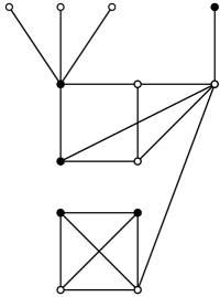
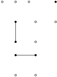
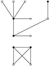
1.2 Main results
Let denote a motif, which is a connected graph on vertices. As mentioned earlier, we do not assume any generative model or additional structures on the parent graph , except that the maximal degree is at most ; this parameter, however, need not be bounded, and one of the goals is to understand how the sample complexity depends on . The goal is to estimate the motif count based on the sampled graph obtained from either subgraph or neighborhood sampling.
Methodologically speaking, Horvitz-Thompson (HT) estimator [20] is perhaps the most natural idea to apply here. The HT estimator is an unbiased estimator of the population total by weighting the empirical count of a given item by the inverse of the probability of observing said item. To be precise, consider estimate the edge count in a graph with edges and maximal degree , the sampling ratio required by the HT estimator to achieve a relative error of scales as , which turns out to be minimax optimal. For being a small constant, this yields a sublinear sample complexity when is large and .
For neighborhood sampling, which is more informative than subgraph sampling since more edges are observed, we show that the optimal sampling ratio can be improved to , which, perhaps surprisingly, is not always achieved by the HT estimator. The main reason for its suboptimality in the high degree regime is the correlation between observed edges. To reduce correlation, we propose a family of linear estimators encompassing and outperforming the Horvitz-Thompson estimator. The key idea is to use the color information indicating which vertices are sampled. For example, in a neighborhood sampled graph it is possible to observe two types of edges: and . The estimator takes a linear combination of the count of these two types of edges with a negative weight on the latter, which, as counterintuitive as it sounds, significantly reduces the variance and achieves the optimal sample complexity.
For general motifs on vertices, for subgraph sampling, it turns out the simple HT scheme for estimating achieves a multiplicative error of with the optimal sampling fraction
which only depends on the size of the motif but not its actual topology. For neighborhood sampling, the situation is more complicated and the picture is less complete. For general , we propose a family of estimators that achieves the sample ratio:
which again only depends on the size of . We conjecture that this is optimal for neighborhood sampling and we indeed prove this for (a) all motifs up to vertices; (b) cliques of all sizes.
Let us conclude this part by providing some intuition on proving the impossibility results. The main apparatus is matching subgraph counts: If two graphs have matching subgraphs counts for all induced (resp. neighborhood) subgraphs up to size , then the total variation of the sampled versions obtained from subgraph (resp. neighborhood) sampling are at . At a high level, this idea is akin to the method of moment matching, which haven been widely used to prove statistical lower bound for functional estimation [26, 5, 39, 21]; in comparison, in the graph-theoretic context, moments correspond to graph homomorphism numbers which are indexed by subgraphs instead of integers [30]. To give a concrete example, consider the triangle motif and take
| (3) |
which have matching subgraph counts up to size two (equal number of vertices and edges) but distinct number of triangles. Then with subgraph sampling, the sampled graph satisfies . For neighborhood sampling, we can take
| (4) |
which have matching degree sequences but distinct number of triangles. In general, these pairs of graphs can be either shown to exist by the strong independence of graph homomorphism numbers for connected subgraphs [12] or explicitly constructed by a linear algebra argument [4]; however, for neighborhood sampling it is significantly more involved as we need to relate the neighborhood subgraph counts to the injective graph homomorphism numbers. Based on these small pairs of graphs, the lower bound in general is constructed by using either or as its connected components.
1.3 Notations
We use standard big- notations, e.g., for any positive sequences and , or if for some absolute constant , or or if . Furthermore, the subscript in indicates that for some constant depending on only. For nonnegative integer , let .
Next we establish some graph-theoretic notations that will be used throughout the paper. Let be a simple, undirected graph. Let denote the number of edges, denote the number of vertices, and be the number of connected components in . The open neighborhood of a vertex is denoted by . The closed neighborhood is defined by . Two vertices and are said to be adjacent to each other, denoted by , if .
Two graphs and are isomorphic, denoted by , if there exists a bijection between the vertex sets of and that preserves adjacency, i.e., if there exists a bijective function such that whenever . If and are vertex-colored graphs with colorings and (i.e., a function that assigns a color to each vertex), then and are isomorphic as vertex-colored graphs, denoted by , if there exist a bijection such that whenever and for all vertices .
Let , , and denote the complete graph (clique), path graph, and cycle graph on vertices, respectively. Let denote the complete bipartite graph (biclique) with edges and vertices. Let denote the star graph on vertices.
Define the following graph operations cf. [37]: The disjoint union of graphs and , denoted , is the graph whose vertex (resp. edge) set is the disjoint union of the vertex (resp. edge) sets of and of . For brevity, we denote by to the disjoint union of copies of . The join of and , denoted by , is obtained from the disjoin union by connecting all and all , that is, , where and and and are disjoint. For example, . For , let denote the resulting graph after deleting all vertices in and all incident edges, and .
We say that is an (edge-induced) subgraph of , denoted by , if and . For any , the subgraph of induced by is denoted by . Let (resp. ) be the number of vertex (resp. edge) induced subgraphs of that are isomorphic to ; in other words,
| (5) | ||||
| (6) |
For example, and . Let denote the clique number, i.e., the size of the largest clique in . Let , and denote the number of edges, triangles and wedges of , which are of particular interest.
1.4 Organization
The paper is organized as follows. In Section 2, we state our positive results in terms of squared error minimax rates and design algorithms that achieve them for subgraph (Section 2.1) and neighborhood (Section 2.2) sampling. Section 3 discusses converse results and states counterpart minimax lower bounds for subgraph (Section 3.2) and neighborhood (Section 3.3) sampling. We further restrict the class of graphs to be acyclic or planar in Section 4 and explore whether such additional structure can be exploited to improve the quality of estimation. In Section 5, we perform a numerical study of the proposed estimators for counting edges, triangles, and wedges on both simulated and real-world data. Finally, in Appendix A, we prove some of the auxiliary lemmas and theorems that were stated in the main body of the paper.
2 Methodologies and performance guarantees
2.1 Subgraph sampling
The motivation for our estimation scheme is based on the observation that any motif count can be written as a sum of indicator functions as in (5). Note that for a fixed subset of vertices , the probability it induces a subgraph in the sampled graph that is isomorphic to is
In view of (5), this suggests the following unbiased estimator of :
| (7) |
We refer to this estimator as the Horvitz-Thompson (HT) estimator [20] since it also uses inverse probability weighting to achieve unbiasedness. The next theorem gives an upper bound on the mean-squared error for this simple scheme, which, somewhat surprisingly, turns out to be minimax optimal within a constant factor as long as the motif is connected.
Theorem 1 (Subgraph sampling).
Let be an arbitrary connected graph with vertices. Let be a graph with maximum degree at most . Consider the subgraph sampling model with sampling ratio . Then the estimator (7) satisfies
Furthermore,
The above result establishes the optimality of the HT estimator for classes of graphs with degree constraints. Since the lower bound construction actually uses instances of graphs containing many cycles, it is a priori unclear whether additional assumptions such as tree structures can help. Indeed, for the related problem of estimating the number of connected components with subgraph sampling, it has been shown that for parent graphs that are forests the sample complexity is strictly smaller [22]. Nevertheless, for counting motifs such as edges or wedges, in Theorem 7 and Theorem 9 we show that the HT estimator (7) cannot be improved up to constant factors even if the parent graph is known to be a forest.
The proof of the lower bound of Theorem 1 is given in Section 3.2. Below we prove the upper bound of the variance:
Proof.
Since is unbiased, it remains to bound its variance. Let , which are iid as . For any , let . Then
Hence
where the penultimate step follows from the fact that the maximum degree of is and, crucially, is connected. ∎
2.2 Neighborhood sampling
Our methodology is again motivated by (5) which represents neighborhood subgraph counts as a sum of indicators. In contrast to subgraph sampling, a motif can be observed in the sampled graph by sampling only some, but not all, of its vertices. For example, we only need to sample one vertex of an edge, or two vertices of a triangle to observe the full motif. More generally, for a subset vertices in , we can determine whether or not if at least vertices from are sampled. This reduces the variance but introduces more correlation at the same time.
Throughout this subsection, the neighborhood sampled graph is again denoted by , and indicates whether a given vertex is sampled.
2.2.1 Edges
We begin by discussing the Horvitz-Thompson type of estimator and why it falls short for the neighborhood sampling model. Analogously to the estimator (7) designed for subgraph sampling, for neighborhood sampling, we can take the observed number of edges and re-weight it according to the probability of observing an edge. Note that with neighborhood sampling, a given edge is observed if and only if at least one of the end points is sampled. Thus, the corresponding Horvitz-Thompson type edge estimator is
| (8) |
which is again an unbiased estimator for . To bound the variance, put and write
where and . For another edge intersecting , we have , by the union bound. Thus the number of non-zero covariance terms is determined by , the number of contained in as subgraphs, and we have
| (9) |
where we used the fact that . Therefore, the variance of the Horvitz-Thompson estimator satisfies
| (10) |
However, as we show next, this estimator is suboptimal when , or equivalently, when the maximum degree exceeds . In fact, the bound (10) itself is tight which can been seen by considering a star graph with leaves, and the suboptimality of the HT estimator is largely due to the heavy correlation between the observed edges. For example, for the star graph, the correlation is introduced through the root vertex, since with probability we observe a full star, and with probability a star with number of black leaves. Thus, the key observation is to incorporate the colors of the vertices to reduce (or eliminate) correlation.
Next, we describe a class of estimators, encompassing and improving the Horvitz-Thompson estimator. Consider
| (11) |
where has the form
| (12) |
here and and are functions of the degree of sampled vertices. For the neighborhood sampling model, this estimator is well-defined since the degree of any sampled vertex is observed without error. It is easy to see that
| (13) |
For simplicity, next we choose and to be constant; in other words, we do not use the degree information of the sampled vertices. This strategy works as long as the maximal degree of the parent graph is known. To illustrate the main idea, we postpone the discussion on adapting to the unknown to Section 2.2.3. With and , the estimator (11) reduces to
| (14) |
which is a linear combination of the counts of the two types of observed edges. In contrast to the HT estimator (8) which treats the two types of edges equally, the optimal choice will weigh them differently. Furthermore, somewhat counter-intuitively, the weights can be negative, which serves to reduce the correlation.
| Graph | ||||
|---|---|---|---|---|
| Probability | ||||
| Value |
In view of (13), one way of making unbiased is to set
| (15) |
Since the unbiased estimator is not unique, we set out to find the one with the minimum variance. Similar to (9), we have
| (16) |
where and are distinct intersecting edges. Using Table 1, we find
In fact, when the unbiased condition (15) is met, the covariance simplifies to . Finally, optimizing the RHS of (16) over subject to the constraint (15), we arrive the following performance guarantee for :
Theorem 2.
Set
| (17) |
Then
| (18) |
Furthermore, if is bounded from one, then
The optimal weights in (17) appear somewhat mysterious. In fact, the following more transparent choice also achieves the optimal risk within constant factors:
-
•
: we can set either or and , that is, we can use either the full HT estimator (8), or the HT estimator restricted to only edges of type , which is the more probable one.
-
•
: we choose and . This is the unique weights that simultaneously kill all covariance terms and, at the same time, achieve zero bias. Note that although zero covariance is always possible, it is at a price of setting , which inflates the variance too much when is small and hence suboptimal when .
It is a priori unclear whether additional structures such as tree or planarity helps for estimating motif counts with neighborhood sampling. Nevertheless, for counting edges, in Theorem 8 we show that the Horvitz-Thompson estimator (7) can only be marginally improved, in the sense that the lower bound continues to hold up to a sub-polynomial factor where is uniformly vanishing as . Similarly, for planar graphs, Theorem 13 shows a similar statement.
2.2.2 Cliques and general motifs
For ease of exposition, we start by developing the methodology for estimating cliques counts. Both the procedure and the performance guarantee readily extend to general motifs.
We now generalize the techniques for counting edges to estimate the number of cliques of size in a given graph. Note that there are two types of colored cliques one observe: (a) : all but one vertex are sampled; (b) : all vertices are sampled, with the first one being more probable when the sampling ratio is small. In the case of triangles, we have and . Analogous to the estimator (14), we take a linear combination of these two types of clique counts as the linear estimator:
| (19) |
Similar to the design principles for counting edges, in the low sampling ratio regime , we implement the Horvitz-Thompson estimator, so that the coefficients scale like ; in the high sampling ratio regime , we choose a negative , which scale as , to reduce the correlation between various observed cliques. However, unlike the case of counting edges, we cannot perfectly eliminate all covariance terms but will be able to remove the leading one.
The following result, which includes Theorem 2 as a special case (), gives the performance guarantee of the estimator (19) and establishes its optimality in the worst case:
Theorem 3 (Cliques).
Set
| (20) |
Then
Furthermore,
Proof.
Let . For any , let . Write
| (21) |
where
Similar to (15), enforcing unbiasedness, we have the constraint , i.e.,
| (22) |
Furthermore, whenever , we have
| (23) | ||||
| (24) |
This follows from evaluating the probability of observing a pair of intersecting cliques with two, one, or zero unsampled vertices. For example, the four summands in (23), in the case of and , correspond to , , , , respectively.
Let for . Denote by the subgraph correspond to two intersecting -cliques sharing vertices. Then
| (25) | ||||
Next consider two cases separately.
Case I: .
In this case we choose and . Then . Furthermore, for the special case of , we have . Thus,
| (26) |
Case II: .
In this high-degree regime, the pairs of cliques sharing one vertex () dominates (i.e., open triangle for counting edge and bowties for counting triangles). Thus our strategy is to choose the coefficients to eliminate the these covariance terms. In fact, (24) for simplifies wonderfully to
Thus we choose and . Hence for all , and
| (27) |
To extend to general motif on vertices, note that in the neighborhood sampled graph, again it is possible to observe fully sampled or partially sampled (with one unsampled vertices) motifs. Consider the following estimator analogous to (19):
| (28) |
where is the count of with all vertices sampled and is the total count of with exactly one unsampled vertices. For instance, if , then and . This example shows that in general, for motifs with less symmetry, there exist multiple partially sampled motifs and in principle they can be weighted differently. However, in (28) we elect to treat them equally, which turns out to be optimal for a wide class of motifs. Let us point out that if the parent graph has more structures, e.g., forest, then distinguishing different partially sampled motifs can lead to strict improvement; see Theorem 10.
The estimator (28) turns out to satisfy the same bound as in the clique case. To see this, note that in (25), the covariance terms are given in (24) which do not depend on the actual motif . Furthermore, the sum of the indicators satisfies the same bound in terms of maximal degree provided that is connected. Using the same optimized coefficients as in (20), the guarantee in Theorem 3 holds verbatim:
| (29) |
We conjecture that, similar to Theorem 1, this rate is optimal as long as the motif is connected. So far we are able to prove this for cliques of all sizes (Theorem 6) and motifs on at most 4 vertices (Appendix D).
2.2.3 Adaptation to the maximum degree
In practice, the bound on the maximum degree is likely unknown to the observer and obtaining a consistent estimate might be difficult if the high-degree vertices are rare. For example, in a star, most of the vertices have degree one expect for the root. Even if a consistent estimate is obtained, it is unclear how to avoid it correlating with the data used to form . Because has the form of a sum, such correlations increase the number of cross terms in its variance decomposition.
To overcome these difficulties, we weight each observed edge according to the size of the neighborhood of its incident vertices. Once a vertex is sampled, its degree is exactly determined and thus incorporating this information does not introduce any additional randomness. This observations leads to the following adaptive estimator which achieves a risk that is similar to the optimal risk in Theorem 2:
Theorem 4.
Let be given in (11) with and . Then for any graph on vertices and maximum degree bounded by , is an unbiased estimator of and
Remark 1.
The variance bound from Theorem 4 is weaker than Theorem 2 in the regime – versus . They have the largest disparity when consists of copies of the star graph , in which case . This is due to the fact that with high probability , all sampled vertices from have degree one. Ideally, we would like to know the degree of the root of the star; however this is impossible unless the root is sampled. Nonetheless, we can still find a good estimate. More generally, in addition to using the degree from a sampled vertex , we may modify the estimator to incorporate degree information from a non-sampled vertex via an unbiased estimate, i.e., . For example, we can redefine from (11) as
3 Lower bounds
Throughout this section we assume that the sampling ratio is bounded away from one.
3.1 Auxiliary results
We start with a result which is the general strategy of proving all lower bounds in this paper. A variant of this result was proved in [22] for the Bernoulli sampling model, however, an examination of the proof reveals that the conclusions also hold for neighborhood sampling. In the context of estimating motif counts, the essential ingredients involve constructing a pair of random graphs whose motif counts have different average values, and the distributions of their sampled versions are close in total variation, which is ensured by matching lower-order subgraphs counts in terms of for subgraph sampling or for neighborhood sampling. The utility of this result is to use a pair of smaller graphs (which can be found in an ad hoc manner) to construct a bigger pair of graphs and produce a lower bound that scales with an arbitrary positive integer .
Theorem 5 (Theorem 11 in [22]).
Let be a graph parameter that is invariant under isomorphisms and additive under disjoint union, i.e., . Fix a subgraph . Let and be integers. Let and be two graphs such that and . Suppose and , where (resp. ) denote the distribution of the isomorphism class of the (subgraph or neighborhood) sampled graph (resp. ). Let denote the sampled version of under the Bernoulli or neighborhood sampling models with probability . Then
| (30) |
where
Next we recall the well-known fact [38, 23] that disconnected subgraphs counts are determined by (fixed polynomials of) connected subgraph counts. The following version is from [22, Corollary 1 and Lemma 9]:
Lemma 1.
Let and be two graphs with vertices and . Suppose for all connected with . Then for all with and, furthermore,
where (resp. ) denote the distribution of the isomorphism class of the subgraph sampled graph (resp. ) with sampling ratio .
The following version is for neighborhood sampling, which will be used in the proof of Theorem 6. We need to develop an analogous result that expresses disconnected neighborhood subgraph counts as polynomials of the connected cones. This is done in Lemma 6 in Appendix A.
Lemma 2.
Let and be two graphs with vertices and . Suppose for all connected, bicolored with . Then
| (31) |
for all with and, furthermore,
| (32) |
where (resp. ) denote the distribution of the isomorphism class of the sampled graph (resp. ) generated from neighborhood sampling with sampling ratio .
Proof.
The first conclusion (31) follows from Lemma 6. For the second conclusion (32), we note that conditioned on vertices are sampled, is uniformly distributed over the collection of all bicolored neighborhood subgraphs with . Thus,
By (31), we conclude that the isomorphism class of and have the same distribution provided that no more than vertices are sampled. Thus, , and consequently, follows from a union bound. ∎
Lemma 3.
For any connected graph with vertices, there exists a pair of (in fact, connected) graphs and , such that and for all connected with .
Proof.
The existence of such a pair and follows from the strong independence222This means that the closure of the range of their normalized version (subgraph densities) has nonempty interior. of connected subgraph counts [12, Theorem 1]. For example, for , we can take the ab hoc construction in (3), which have equal number of vertices and edges but distinct number of triangles. Alternatively, next we provide an explicit construction using a linear algebra argument which is similar to that of [12, Theorem 3] and [4, Section 2]. Let denote all distinct (up to isomorphism) induced connected subgraph of , ordered in increasing number of edges (arbitrarily among graphs with the same number of edges) so that is an isolated vertex and . Then the matrix with is upper triangular with strictly positive diagonals. Thus is invertible and the entries of are rational. Let , where . Then since . Let , where is the lowest common denominator of the entries of . Now define and as the disjoint union with weights given by the vector :
| (33) |
By design, any connected induced subgraph of and with at most vertices belongs to . For any , since is connected, we have , and and . For example, for , such a solution is given by:
which have matching subgraphs of order three (vertices, edges and triangles). For a construction for general cliques, see [22, Eq. (47)]. ∎
Next we present graph-theoretic results that are needed for proving lower bound under the neighborhood sampling model. First, we relate the neighborhood subgraph counts to the usual subgraph . Since is essentially subgraph counts with prescribed degree for the sampled vertices (cf. [29, p. 62]), this can be done by inclusion-exclusion principle similar to (1) that expresses the induced subgraph counts in terms of the subgraph counts ; however, the key difference here is that the size of the subgraphs that appear in the linear combination is not bounded a priori. For example,
| number of degree- vertices in | |||
where is the star graph with leaves. The following lemma is a general statement:
Lemma 4.
Let be a bicolored connected neighborhood graph and denote the uncolored version. Then for any ,
| (34) |
where the sum is over all (uncolored) obtained from by either adding edges incident to the black vertices in or adding vertices connected to black vertices in . In particular, the coefficients do not depend on .
Proof.
The proof is by the inclusion-exclusion principle and essentially similar to the argument in Section 5.2, in particular, the proof of Proposition 5.6(b) in [29].
Recall the definition of the subgraph count in (6) in terms of counting distinct subsets. It will be convenient to work with the labeled version counting graph homomorphisms. The following definitions are largely from [29, Chapter 5]. We say is an injective homomorphism from to , if is injective, and if . Denote by the number of injective homomorphisms from to . Then , where denotes the number of automorphisms (i.e. isomorphisms to itself) for . Furthermore, for neighborhood subgraph , denotes the number of automorphisms for that also preserve the colors. For example, and . Throughout the proof, always denotes an injection.
We use the following version of the inclusion-exclusion principle [29, Appendix A.1]. Let be a ground set and let be a collection of sets. For each , define and ; in words, denotes those elements that belong to exactly those for and none other. Then we have
| (35) | ||||
| (36) |
Fix . Let denote the collection of (uncolored) subgraphs that are “extensions” of , obtained from by either adding edges between the black vertices in or adding vertices attached to black vertices in . For example, for , we have is the collection of all stars. Let the be the maximal subgraph of that is in ; in other words, , for any other containing as a subgraph.
The next result is the counterpart of Lemma 3, which shows the existence of a pair of graphs with matching lower order neighborhood subgraph counts but contain distinct number of copies of a certain motif; however, unlike Lemma 3, so far we can only deal with the clique motifs. For example for , we can use the ad hoc construction in (3); both graphs have the same degree sequence but distinct number of triangles. For , we can choose
| (37) | ||||
It it straightforward (although extremely tedious!) to verify that for all neighborhood subgraphs with at most 2 black vertices. The general result is as follows:
Lemma 5.
There exists two graphs and such that and for all neighborhood subgraphs such that .
Proof.
First we show that there exist a pair of graphs and such that for all connected graphs with at most vertices expect for the clique , and for all connected graphs with more than vertices. Analogous to the proof of Lemma 3, this either follows from the strong independence of injective graph homomorphism numbers [12], or from the following linear algebra argument. Let denote all distinct (up to isomorphism) connected graphs of at most vertices. Order the graphs in increasing number of edges (arbitrarily among graphs with the same number of edges) so that is an isolated vertex and . Then the matrix with is upper triangular with strictly positive diagonals. Then and can be constructed from the vector similar to (33); see (37) for a concrete example for . By design, each connected component of and has at most vertices, we have for all connected with .
Next we show that the neighborhood subgraph counts are matched up to order . For each neighborhood subgraph with , by Lemma 4, we have , where the coefficients are independent of , and contains all subgraphs obtained from by adding edges incident to black vertices in or attaching vertices to black vertices in . The crucial observation is two-fold: (a) since , there exists at least a pair of white vertices in , which are not connected. Since no edges are added between white vertices, the collection excludes the full clique ; (b) for each , if contains more than vertices, then ; if contains at most vertices (and not by the previous point), then by design. Therefore we conclude that for all neighborhood subgraphs with . ∎
3.2 Subgraph sampling
Next we prove the lower bound part of Theorem 1:
Proof.
Throughout the proof, we assume that both and are at least some sufficiently large constant that only depends on and we use to denote constants that possibly depend on only. We consider two cases separately.
Case I: .
Case II: .
To apply Lemma 9, we construct a pair of graphs and with maximum degree such that , and . Choosing for some small constant and applying Theorem 5, we obtain
| (39) |
Combining (38) and (39) completes the proof of the lower bound of Theorem 1.
It remains to construct and . The idea of the construction is to expand each vertex in into an independent set, which was used in the proof of [12, Lemma 5]. Here, we also need to consider the possibility of expanding into a clique. Next consider two cases:
Suppose satisfies the “distinct neighborhood” property, that is, for each , is a distinct subset of . Such includes cliques, paths, cycles, etc. Pick an arbitrary vertex . Let be a collection of disjoint subsets, so that and , where is a constant that only depends on such that . Define a graph with vertex set by connecting each pair of and whenever . In other words, is obtained by blowing up each vertex in into an independent set and each edge into a complete bipartite graph. Repeating the same construction with replaced by yields , in which case consists of isolated vertices. By construction, the maximum degree of both graph satisfies is at most . Note that . Thus the sampled graph of and have the same law provided that none of the vertices in is sampled. Applying Lemma 9, we conclude that for all , where is a constant depending only on .
Furthermore,
where (a) follows from the fact that contains isolated vertices whenever while is connected by assumption. Note that since , if , then there exists such that belong to the same independent set for some . By construction, and have the same neighborhood, contradicting . Thus, we conclude that . For , we have
and, similarly, .
Next suppose that does have distinct neighborhoods, thus there exist with such that the neighborhood are identical, denoted by . Let is an induced (by ) subgraph of . We define with vertex set by the same procedure as above, except now all vertices are expanded into a clique, with and for . Finally, as before, we connect each pair of and whenever . Define by repeating the same construction with replaced by . Analogous to the above we have and it remains to show that . Indeed, for any set of vertices that does not include any vertex from , since forms a clique and form an independent set in , the number of induced in is strictly less than that in . Thus, there exists no such that is isomorphic to , and hence . Entirely analogously, we have . ∎
3.3 Neighborhood sampling
To illustrate the main idea, we only prove the lower bound cliques. The proof for other motifs (of size up to four) is similar but involves several ad hoc constructions; see Appendix D.
Theorem 6 (Cliques).
For neighborhood sampling with sampling ratio ,
Proof.
For the lower bound, consider two cases. For simplicity, denote the minimax risk on the left-hand side by .
Case I: .
Case II: .
We use a different construction. Let for some small constant . Let and be the two graphs from Lemma 5 such that and for all neighborhood subgraphs with . By Lemma 2, we have . Next we amplify the gap by expanding each vertex into an independent set, similar in what is done in the proof of Theorem 1. For each vertex in , we associate distinct isolated vertices, and connect each pair of vertices by an edge if and only if they were connected in . This defines a new graph with vertices and similarly we construct from . In this way, the subgraph counts of and also match up to order , and, in view of Lemma 2, . Furthermore, the number of cliques satisfies and . Thus, . Applying Theorem 5 with yields , where the last step follows from the assumption that . ∎
4 Graphs with additional structures
In this section, we explore how estimation of motif counts can be improved by prior knowledge of the parent graph structure. In particular, for counting edges, we show that even if the parent graph is known to be a forest a priori, for neighborhood sampling, the bound in Theorem 2 remains optimal up to a subpolynomial factor in . Similarly, for subgraph sampling, we cannot improve the rate in Theorem 1. We also discuss some results for planar graphs. In what follows, we let and denote the collection of all forests and planar graphs, respectively.
The next results shows that for estimating edge counts, even if it is known a priori that the parent graph is a forest, the risk in Theorem 1 and Theorem 2 cannot be improved in terms of the exponents on . The proofs of all the following results are given in Appendix B.
Theorem 7.
For subgraph sampling with sampling ratio ,
| (40) |
Theorem 8.
For neighborhood sampling with sampling ratio ,
where is with respect to and uniform in all other parameters.
For estimating the wedge count under subgraph sampling, the following result shows that the risk in Theorem 1 cannot be improved even if we know the parent graph is a forest.
Theorem 9.
For subgraph sampling with sampling ratio ,
| (41) |
On the other hand, for neighborhood sampling, the tree structure can be exploited to improve the rate. Analogous to (14), we consider an estimator of the form
| (42) |
If we weight and equally, i.e., , this estimator reduces to (28) and hence inherits the same performance guarantee in (29), which by Theorem 15, is optimal. However, as will be seen in Theorem 11, there is added flexibility by this three-parameter family of estimators that produces improved bounds when the parent graphs satisfies certain additional structure. It should also be mentioned that the alternative choices , , and yield the same performance bound as in (29).
For this next result, we show that we can improve the performance of the wedge estimator (42) if the parent graph is a forest by choosing alternate values of the parameters: , , and . These choices eliminate the largest term in the variance of (42), which is proportional to . We immediately get the following variance bound:
| (43) |
Note also that whenever is a forest. Hence another estimator we can use is which has variance of order . Putting this all together, we obtain the following result.
Theorem 10.
For neighborhood sampling with sampling ratio ,
The next theorem shows that the minimax bound from Theorem 10 is optimal.
Theorem 11.
For neighborhood sampling with sampling ratio and ,
In the context of estimating triangles, the next set of results show that planarity improves the rates of estimation for both sampling models. Despite the smaller risk however, for subgraph sampling, the optimal estimator is still the Horvitz-Thompson type.
Theorem 12.
For subgraph sampling with sampling ratio ,
Theorem 13.
For neighborhood sampling with sampling ratio ,
5 Numerical experiments
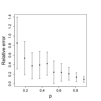
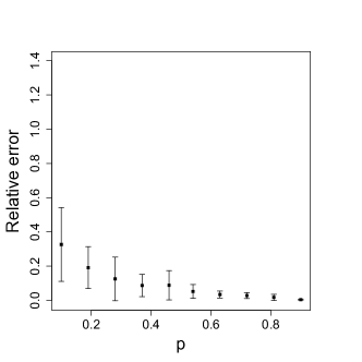
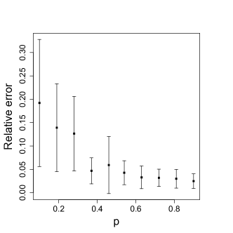
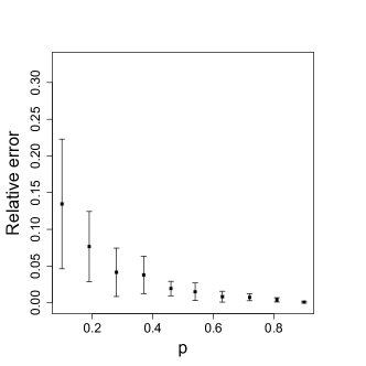
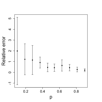
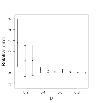
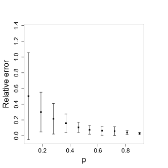
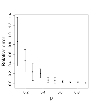
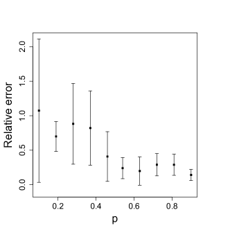
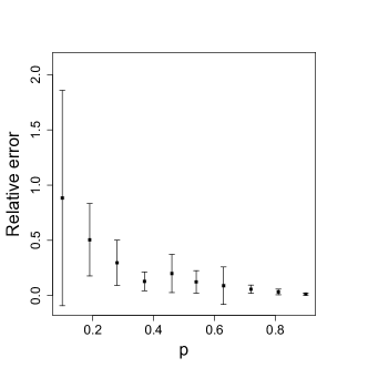
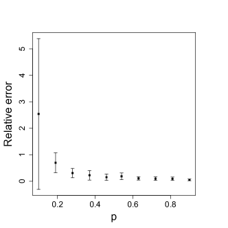
We perform our experiments on both synthetic and real-world data. For the synthetic data, we take as our parent graph a realization of an Erdös-Rényi graph for various choices of parameters. For the real-world experiment, we study the social networks of survey participants using a Facebook app [28]. This dataset contains 10 ego-networks (the closed neighborhood of a focal vertex (“ego”) and any edges between vertices in its neighborhood) of various sizes, although we only use three of them as our parent graphs . The error bars in the following figures show the variability of the relative error of edges, triangles, and wedges over 10 independent experiments of subgraph and neighborhood sampling on a fixed parent graph . The solid black horizontal line shows the sample average and the whiskers show the mean the standard deviation.
Specifically, for subgraph sampling, we always use the HT estimator (7). For neighborhood sampling, for counting triangles or wedges, we use the estimator (28) with choice of parameters given in Theorem 3 and for counting edges we use the adaptive estimator in Theorem 4. The relative error for estimating the number of edges, triangles, and wedges are given in Fig. 2– Fig. 4, respectively.
As predicted by the variance bounds, the estimators based on neighborhood sampling perform better than subgraph sampling. Furthermore, there is markedly less variability across the 10 independent experiments in neighborhood sampling. In all plots, however, this variability decreases as grows. Furthermore, in accordance with our theory, counting bigger motifs (involving more vertices) is subject to more variability, which is evidenced in the plots for triangles and wedges by the wider spread in the whiskers.

6 Discussion
We conclude the paper by mentioning a number of interesting questions that remain open:
-
•
As mentioned in the introduction, a more general (and powerful) version of the neighborhood sampling model is to observe a labeled radius- ball rooted at a randomly chosen vertex [29]. The current paper focuses on the case of . For , we note for example that a triangle could be observed simply by sampling only one of its vertices, i.e., . Thus, a Horvitz-Thompson type of estimator is and the variance scales as . When is small, this outperforms the neighborhood sampling counterpart () in Theorem 3, where the variance scales as . Understanding the statistical limits of -hop neighborhood sampling is an interesting and challenging research direction. In particular, the lower bound will potentially involve more complicated graph statistics as opposed neighborhood subgraph counts.
-
•
In this paper we have focused on counting motifs as induced subgraphs. As shown in (1), subgraph counts can be expressed linear combinations of induced subgraph counts. However, this does not necessarily mean their sample complexity are the same. Although we do not have a systematic understanding so far, here is a concrete example that demonstrates this: consider estimating the number of (not necessarily) 4-cycles with neighborhood sampling. Note that to observe a one only need to sample the two diagonal vertices. Thus, a simple unbiased estimator is , whose variance scales as and is much smaller than the best error rate for estimating induced ’s which scales as , as given by Theorem 6. The explanation for this phenomenon is that although we have the deterministic relationship and each of the three subgraph counts can be estimated at the rate of , the statistical errors cancel each other and result in a faster rate.
Appendix A Auxiliary lemmas
Lemma 6 (Kocay’s Edge Theorem for Colored Graphs).
Let be a bicolored disconnected graph. Then can be expressed as a polynomial, independent of , in , where is bicolored, connected, and . Moreover, if is a term in the polynomial, then and the corresponding coefficient is bounded by . The number of terms in the polynomial representation is bounded by the number of -tuples of all bicolored neighborhood subgraphs such that and .
Proof.
For a disconnected graph , note that can be decomposed into two graphs and , where is connected and . Then,
| (44) |
where the sum runs over all graphs with and is the number of decompositions of into and into (not necessarily disjoint) such that and .
The only disconnected graph satisfying the above decomposition property for is , and hence
| (45) |
where and the sum ranges over all that are either connected and or disconnected and . Furthermore, each can be bounded by the number of ways of decomposing a set of size into two sets (with possible overlap), or .
We will now prove the following claim using induction. Let be a bicolored disconnected graph. For each ,
| (46) |
where contains at least one disconnected for which , , , and the number of terms is bounded by the number of -tuples of all bicolored neighborhood graphs such that and .
The base case is established by decomposing into two graphs and with connected and and applying (45) with , , and .
Next, suppose (46) holds. Then applying (45) to each disconnected , we have
| (47) |
Note that and if is disconnected, then . Finally, we observe that (47) has the form
| (48) |
where contains at least one disconnected for which , , , and . The number of terms is bounded by the number of -tuples of all bicolored neighborhood graphs such that and . Repeat this until and so that the right hand side of (46) contains no disconnected in its terms. ∎
Lemma 7.
Let and be two graphs on vertices. Suppose there exists a constant and positive integer such that for each connected subgraph ,
Then for each subgraph ,
where is the number of -tuples of all bicolored neighborhood graphs such that and or .
Proof.
Let be a disconnected subgraph. By Lemma 6, , where , is connected, , and the number of terms is bounded by . Thus, using the fact that if and are positive real numbers, , we have
where is an ordering of . Next, we use the fact that to bound
Since , the above is further bounded by . Thus,
∎
Next we present two results on the total variation that will be used in the regime of . The main idea is the following: if a subset of vertices are not sampled, for subgraph sampling, in the observed graph we delete all edges incident to , i.e., the edge set of , and for neighborhood sampling, we delete all edges within , that is, the edge set of . Therefore, for two parent graphs, if missing leads to isomorphic graphs, then by a natural coupling, the total variation between the sampled graphs is at most the probability that is not completely absent in the sample.
Lemma 8.
Let for integer between zero and . Consider the neighborhood sampling model with sampling ratio . Suppose and both and are at most . For neighborhood sampling with sampling ratio , there exists such that
Proof.
Note that is the union of two complete bipartite graphs. Suppose that none of the “left” side vertices are sampled. Then can be described by , where . Thus, if , then
Furthermore, observe that
where
This shows that if and both and are , then is less than a constant less than one. ∎
Lemma 9.
Let , , and be an arbitrary graphs and let for and . If , then for neighborhood sampling with sampling ratio ,
| (49) |
More generally, for and defined on the same set of vertices, if is such that and are isomorphic, then (49) holds with .
Proof.
Suppose that none of the vertices in or are sampled. Then and are isomorphic to each other. Thus,
The second claim follows from the same argument. ∎
The following lemma, which was used in the proof of Theorems 8 and 10, relies on a number-theoretic fact:
Lemma 10.
There exist two sequences of integers and such that
and
where stands for the least common multiple. Moreover, there exists universal constants and such that
| (50) |
Proof.
We first introduce the quantity
The key observation is that for all polynomials with degree less than or equal to . Hence we can set
and
where . A well-known number theoretic fact is that the least common multiple of the integers is in fact significantly smaller than their product. In fact, we have the estimates [33], [19]
which shows (50). ∎
Lemma 11.
Proof.
There are four types of connected subgraphs of and : edge with one black vertex, edge with two black vertices, , with white center, , with black center. If is an edge with one black vertex and . If is an edge with two black vertices and . If with white center, then and and furthermore,
If with black center, then
We find that and .
Let . Then
where the sum runs over all bicolored graphs with at most black vertices. By Lemma 7, for each subgraph ,
where we used the bound . Hence,
for some constant and provided . ∎
Lemma 12.
Proof.
There are two types of connected subgraphs of and : , with white center and , with black center. If with white center, then and and furthermore, since for ,
If with black center, then
We find that and .
Let . Then
where the sum runs over all bicolored graphs with at most black vertices. By Lemma 7, for each subgraph with ,
where we used the bound . Hence,
for some constant and provided . ∎
Lemma 13.
There exists two planar graphs and on order vertices with matching degree sequences and maximum degree equal to such that for neighborhood sampling with sampling ratio , and provided . Furthermore, there exists two planar graphs and on order vertices such that for neighborhood sampling with sampling ratio , and .
Proof.
The proof follows from an examination of the two graphs below. Note that for all connected with and since for all connected with , it follows from Lemma 7 with that for all with . Thus,
provided . The identity follows from the fact that and have matching degree sequences (corresponding to matching subgraphs from neighborhood sampling with one vertex).
| Copies | Components |
|---|---|
| 1 | 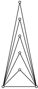 |
| 2 | 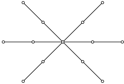 |
| 2 | 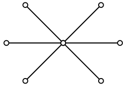 |
 |
|
 |
| Copies | Components |
|---|---|
| 1 | |
| 2 | 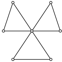 |
| 1 | 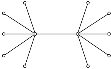 |
 |
|
 |
For the second statement, consider two planar graphs and on vertices, where consists of triangles sharing a common edge, and consists of wedges sharing a pair of non-adjacent vertices; see Fig. 5 for an illustration for .


Note that if neither of the two highest-degree vertices in each graph (degree in and degree in ) are sampled and all incident edges removed, the two graphs are isomorphic. This shows that . Also, note that and . ∎
Appendix B Additional proofs
Proof of Theorems 7, 9, and 12.
The upper bounds are achieved by Horvitz-Thompson estimation as in Theorem 1. However, for Theorem 9, we are able to achieve a smaller variance because is of order for planar instead of and hence . For the lower bound, the proof follows the same lines as Section 3.2 in that we use two different constructions depending on whether or .
For edges, let and with for some small constant . Then .
For wedges, when , let and . Then . When , let and . Then . Finally set for some universal constant .
Finally, for triangles, let be the graph which consists of triangles that share the same edge plus isolated vertices. Let be the graph which consists of two star graphs with an edge between their roots. Choose for some small universal constant . Then . ∎
Proof of Theorem 8.
Let and be two sequences of integers defined by and , where is as in Lemma 10. Consider the disjoint union of stars
for integer .
Note, for example, that and . Thus, for some universal . Note that
and by Lemma 11 there exists universal such that
provided .
By Theorem 5, we have
where
for some universal constants provided . Next, choose
| (51) |
Taking yields the desired lower bound. ∎
Proof of Theorem 11.
Let and be two sequences of integers defined by and , where is as in Lemma 10. Let
for integer . Note, for example, that , , and . This means that for some universal . Note that
By Lemma 12, we have that for some universal . By Theorem 5, we have
where
for some universal constant . Next, choose and when for some universal constant . For and , we use Lemma 8 with and . Then and , and . By Theorem 5, we have . ∎
Proof of Theorem 13.
Let denote the minimax risk. The bound follows immediately from Theorem 6 with . For the other regimes, we modify the estimator (21) from Theorem 3. To accomplish this, observe that is of order for planar , since the number of triangles that share a common vertex is at most . Choosing so that, in the notation of the proof of Theorem 3, and , we have . This yields the bound . Thus, . For the lower bound, consider two cases:
Case I: .
Case II: .
We use the second statement of Lemma 13 which guarantees the existence of two planar graphs and on order vertices such that and . Choosing yields the lower bound . ∎
Proof of Theorem 4.
To make unbiased, in view of (13), we set
This determines
An easy calculation shows that
and if and in , then
Otherwise, if and do not intersect. Thus,
| (52) |
where denotes the cardinality of . To gain a better idea for how to choose , we first suppose that . Thus, (52) reduces to the mean square error of (11) or
Next, let us minimize the above expression over all . Doing so with
yields
| (53) |
Note that is a convex combination of and . These are the values that yield the risk bound for the non-adaptive estimator (11) in Theorem 2, viz.,
Of course, this choice of is not feasible since it depends on the unknown quantities and . However, noting that and inspires us to define
With this choice of , we will verify that the variance and covariance terms in (52) also yield the rate (18). Note that
where the second last inequality follows from the concavity of for . The variance term has the bound
which follows from and . ∎
Appendix C Neighborhood sampling without colors
In this appendix we demonstrate the usefulness of the color information (namely, which vertices are sampled) in neighborhood sampling by showing that without observing the colors, the performance guarantees in Theorem 2 are no longer unattainable in certain regimes.
Theorem 14.
Let denote the collection of all forests. Consider the neighborhood sampling model without observing the colors . Then
| (54) |
Proof.
Let , where and set . Note that for each , . Thus, if , where are independent and for , then
By the minimax theorem,
where and the second to last line follows from Lemma 14 below. ∎
Remark 2.
Note that when and , the minimax lower bound (54) is strictly greater than the minimax risk in Theorem 8, thus confirming the intuition that the knowledge of which vertices are sampled provide useful information. On the other hand, the Horvitz-Thompson estimator (8) can be implemented without the color information and achieve the error bound in (10). Comparing with Theorem 1, we conclude that neighborhood sampling is at least as informative as subgraph sampling, even if the colors are not observed. This is intuitive because neighborhood sampling reveals more edges from the parent graph.
Lemma 14.
Given , let be distributed according to . Assume that . Then
| (55) |
Moreover, the minimax rate is achieved by the estimator .
Appendix D Lower bounds for other motifs
Theorem 15 (Wedges).
For neighborhood sampling with sampling ratio ,
Proof.
For the lower bound, consider two cases:
Case I: .
Let and . For each node in the original graph, we associate distinct isolated vertices and connect each pair of vertices by an edge if and only if they were connected in the original graph. Call these expanded graphs and . Note that and that have matching degree sequences and hence . Furthermore, . If , then by Theorem 5 with , .
Case II: .
Lower bound for motifs of size four
It remains to show that holds the result in Theorem 6 that holds for , namely,
| (59) |
continues to hold for and . For the case of , the construction for in (37) works simultaneously for all motifs, because each motif is contained in one of and and not the other. Next we consider the case of . The construction is ad hoc and similar to those in Theorem 1 and Theorem 3.
-
•
For , we use the clique construction: label the root as and the leaves as . Define the graph as follows: Expand into a clique of size , and for , expand each into a clique of size . Connect each pair of vertices and for if and only if and are connected in the motif . This defines a graph on vertices. Repeat the same construction with replaced by , where the degree-one vertex is . Note that if we remove the edges between the set of vertices , for and the resulting graph is isomorphic. Thus by Lemma Lemma 9, we have if . Furthermore, note that and . Finally, taking for some small constant and invoking Theorem 5, we obtain the desired lower bound in (59).
-
•
For , use the same construction as above with and swapped.
-
•
For , we repeat the clique construction of with being any of the degree-three vertices in , and of with ; in other words, we simply have .
-
•
For , we repeat the clique construction of with being any vertex in , and of with , with being the degree-two vertices.
References
- [1] Maryam Aliakbarpour, Amartya Shankha Biswas, Themis Gouleakis, John Peebles, Ronitt Rubinfeld, and Anak Yodpinyanee. Sublinear-time algorithms for counting star subgraphs via edge sampling. Algorithmica, pages 1–30.
- [2] Coren L. Apicella, Frank W. Marlowe, James H. Fowler, and Nicholas A. Christakis. Social networks and cooperation in hunter-gatherers. Nature, 481(7382):497–501, 01 2012.
- [3] Peter J. Bickel, Aiyou Chen, and Elizaveta Levina. The method of moments and degree distributions for network models. Ann. Statist., 39(5):2280–2301, 2011.
- [4] Norman Biggs. On cluster expansions in graph theory and physics. Quart. J. Math. Oxford Ser. (2), 29(114):159–173, 1978.
- [5] T.T. Cai and M. G. Low. Testing composite hypotheses, Hermite polynomials and optimal estimation of a nonsmooth functional. 39(2):1012–1041, 2011.
- [6] Michael Capobianco. Estimating the connectivity of a graph. In Y. Alavi, D. R. Lick, and A. T. White, editors, Graph Theory and Applications, pages 65–74, Berlin, Heidelberg, 1972. Springer Berlin Heidelberg.
- [7] Arun Chandrasekhar and Randall Lewis. Econometrics of sampled networks. 2011.
- [8] Hao Chen, Nancy Zhang, et al. Graph-based change-point detection. The Annals of Statistics, 43(1):139–176, 2015.
- [9] Lynna Chu and Hao Chen. Asymptotic distribution-free change-point detection for modern data. arXiv preprint arXiv:1707.00167, 2017.
- [10] Graham Cormode and Nick Duffield. Sampling for big data: a tutorial. In Proceedings of the 20th ACM SIGKDD International Conference on Knowledge Discovery and Data Mining, pages 1975–1975. ACM, 2014.
- [11] Talya Eden, Amit Levi, Dana Ron, and C. Seshadhri. Approximately counting triangles in sublinear time. In 2015 IEEE 56th Annual Symposium on Foundations of Computer Science—FOCS 2015, pages 614–633. IEEE Computer Soc., Los Alamitos, CA, 2015.
- [12] Paul Erdös, László Lovász, and Joel Spencer. Strong independence of graphcopy functions. In Graph theory and related topics (Proc. Conf., Univ. Waterloo, Waterloo, Ont., 1977), pages 165–172. Academic Press, New York-London, 1979.
- [13] Uriel Feige. On sums of independent random variables with unbounded variance and estimating the average degree in a graph. SIAM J. Comput., 35(4):964–984, 2006.
- [14] Chao Gao and John Lafferty. Testing network structure using relations between small subgraph probabilities. arXiv preprint arXiv:1704.06742, 2017.
- [15] Oded Goldreich and Dana Ron. Approximating average parameters of graphs. Random Structures Algorithms, 32(4):473–493, 2008.
- [16] Mira Gonen, Dana Ron, and Yuval Shavitt. Counting stars and other small subgraphs in sublinear-time. SIAM J. Discrete Math., 25(3):1365–1411, 2011.
- [17] Jing-Dong J Han, Denis Dupuy, Nicolas Bertin, Michael E Cusick, and Marc Vidal. Effect of sampling on topology predictions of protein-protein interaction networks. Nature Biotechnology, 23(7):839, 2005.
- [18] Mark S. Handcock and Krista J. Gile. Modeling social networks from sampled data. Ann. Appl. Stat., 4(1):5–25, 2010.
- [19] Denis Hanson. On the product of the primes. Canad. Math. Bull., 15:33–37, 1972.
- [20] Daniel G Horvitz and Donovan J Thompson. A generalization of sampling without replacement from a finite universe. Journal of the American Statistical Association, 47(260):663–685, 1952.
- [21] Jiantao Jiao, Kartik Venkat, Yanjun Han, and Tsachy Weissman. Minimax estimation of functionals of discrete distributions. IEEE Transactions on Information Theory, 61(5):2835–2885, 2015.
- [22] Jason M. Klusowski and Yihong Wu. Estimating the number of connected components in a graph via subgraph sampling. arXiv preprint arXiv:1801.04339, 2018.
- [23] W. L. Kocay. Some new methods in reconstruction theory. In Combinatorial mathematics, IX (Brisbane, 1981), volume 952 of Lecture Notes in Math., pages 89–114. Springer, Berlin-New York, 1982.
- [24] Eric D Kolaczyk. Statistical Analysis of Network Data: Methods and Models. Springer Science & Business Media, 2009.
- [25] Eric D. Kolaczyk. Topics at the Frontier of Statistics and Network Analysis: (Re)Visiting the Foundations. SemStat Elements. Cambridge University Press, 2017.
- [26] Oleg Lepski, Arkady Nemirovski, and Vladimir Spokoiny. On estimation of the norm of a regression function. 113(2):221–253, 1999.
- [27] Jure Leskovec and Christos Faloutsos. Sampling from large graphs. In Proceedings of the 12th ACM SIGKDD International Conference on Knowledge Discovery and Data Mining, pages 631–636. ACM, 2006.
- [28] Jure Leskovec and Andrej Krevl. SNAP Datasets: Stanford large network dataset collection. http://snap.stanford.edu/data/egonets-Facebook.html, June 2014.
- [29] László Lovász. Large Networks and Graph Limits, volume 60. American Mathematical Society, 2012.
- [30] László Lovász and Balázs Szegedy. The graph theoretic moment problem. arXiv preprint arXiv:1010.5159, 2010.
- [31] Ron Milo, Shai Shen-Orr, Shalev Itzkovitz, Nadav Kashtan, Dmitri Chklovskii, and Uri Alon. Network motifs: simple building blocks of complex networks. Science, 298(5594):824–827, 2002.
- [32] Elchanan Mossel, Joe Neeman, and Allan Sly. Reconstruction and estimation in the planted partition model. Probab. Theory Related Fields, 162(3-4):431–461, 2015.
- [33] M. Nair. On Chebyshev-type inequalities for primes. Amer. Math. Monthly, 89(2):126–129, 1982.
- [34] Natasa Pržulj, Derek G Corneil, and Igor Jurisica. Modeling interactome: scale-free or geometric? Bioinformatics, 20(18):3508–3515, 2004.
- [35] Peter Uetz, Loic Giot, Gerard Cagney, Traci A Mansfield, Richard S Judson, James R Knight, Daniel Lockshon, Vaibhav Narayan, Maithreyan Srinivasan, Pascale Pochart, et al. A comprehensive analysis of protein–protein interactions in saccharomyces cerevisiae. Nature, 403(6770):623, 2000.
- [36] Stanley Wasserman and Katherine Faust. Social network analysis: Methods and applications, volume 8. Cambridge university press, 1994.
- [37] Douglas B. West. Introduction to graph theory. Prentice Hall, Inc., Upper Saddle River, NJ, 1996.
- [38] Hassler Whitney. The coloring of graphs. Ann. of Math. (2), 33(4):688–718, 1932.
- [39] Yihong Wu and Pengkun Yang. Minimax rates of entropy estimation on large alphabets via best polynomial approximation. IEEE Transactions on Information Theory, 62(6):3702–3720, 2016.